Getting the Agent to Wait††thanks: We owe the title of this paper to Orlov, Skrzypacz and Zryumov’s work! We thank several seminar and conference participants as well as Nageeb Ali, Arjadha Bardhi, James Best, Lukas Bolte, Joyee Deb, Alexey Kushnir, George Loewenstein, and Vasiliki Skreta.
Abstract
We examine the strategic interaction between an expert (principal) maximizing engagement and an agent seeking swift information. Our analysis reveals: When priors align, relative patience determines optimal disclosure—impatient agents induce gradual revelation, while impatient principals cause delayed, abrupt revelation. When priors disagree, catering to the bias often emerges, with the principal initially providing signals aligned with the agent’s bias. With private agent beliefs, we observe two phases: one engaging both agents, followed by catering to one type. Comparing personalized and non-personalized strategies, we find faster information revelation in the non-personalized case, but higher quality information in the personalized case.
1 Introduction
Maximizing engagement is a central objective across many economic settings, from traditional expert services such as management consulting and legal advice to modern digital platforms with content provision and recommender systems. In these contexts, an expert (principal) aims to prolong user engagement to maximize value extraction, while the user (agent) incurs costs from extended information acquisition periods. In this paper, we develop a general framework for analyzing such interactions.
To do so, we consider a model in which a principal and an agent interact through engagement. The agent engages to collect information about a payoff-relevant decision, while the principal aims solely to maximize the duration of this engagement. This engagement is irreversible and represents a trade-off: it is costly for the agent but valuable for the principal. A key feature of our model is allowing for the agent to have a different prior from the principal which could be publicly observable to the principal (in the spirit of Aumann (1976)’s agree-to-disagree framework) or privately known to the agent. This approach enables us to explore how differences in beliefs and information asymmetry impact optimal engagement strategies.
Our analysis reveals three key patterns that determine optimal information provision in this environment. First, the relative patience of the agent and principal determines whether information is revealed abruptly or gradually. Second, when the agent and the principal agree to disagree on their prior, it is often the case that optimal disclosure features catering to the bias – the principal first reveals the state towards which the agent is more biased towards. Third, when the agent’s belief is private information, there is a trade-off between speed and quality as information is revealed faster but engagements end with more uncertain beliefs.
When the principal and the agent share the same prior, the main determinant of information disclosure is how the cost of engagement for the agent evolves over time relative to its benefit for the principal. More specifically, suppose that both the principal and the agent use exponential discounting. The principal then values each moment of engagement at an exponentially declining rate, i.e., he values early engagement more than later ones. When the agent is more impatient than the principal, exponential discounting implies that the relative cost of engagement decreases over time. This in turn means that by some gradual revelation early on, the principal is able to postpone revelation for a time when the cost of engagement is lower for the agent. Technically, when the discount rate of the principal is lower than that of the agent, the payoff of the agent is convex in the payoff of the principal, and thus the agent and principal both benefit from random or gradual disclosure. This disclosure takes the form of a Poisson arrival of the news. In contrast, when the agent is more patient, the cost of being engaged increases for the agent relative to the benefit for the principal, which will lead to abrupt information revelation.
The equilibrium dynamics shift significantly when the principal and agent have different prior beliefs. This divergence introduces a crucial asymmetry in how each party values engagement across different states. Consider a scenario where the agent is more optimistic about state than the principal. In this case, revealing information about carries higher value for the agent but represents a lower cost for the principal. This asymmetry arises because the principal, believing to be less probable, perceives the promise of revelation in this state as less likely to materialize than the agent anticipates. Consequently, promising to disclose information about becomes a cost-effective strategy for maintaining agent engagement. This is what we refer to as catering to the bias.
When the agent is more patient, catering to the bias always occurs. There is a phase in which no information is revealed; mirroring the optimal disclosure pattern under shared priors. This is followed by a second phase where the state towards which the agent is more biased is gradually revealed according to a time-varying Poisson rate. Finally, at the end of the second phase, the other state is revealed instantaneously.
With a more patient principal, catering to the bias would occur when the difference between the prior of the agent and the principal is sufficiently large. In this case, a frontier steady state pair of beliefs exists such that the beliefs are going to converge to it. When the priors agree, this will be the point of maximum uncertainty and maximum engagement. Along this frontier, the optimal disclosure involves symmetric, constant-rate Poisson disclosure of both states. As such, beliefs remain stable on the frontier over time until a disclosure event occurs.
The evolution of beliefs (probability that for the agent (x-axis) and the principal (y-axis)) away from this steady state is depicted in Figure 1. Below the stationary engagement curve, the state is revealed according to a time-varying Poisson process, and above it the state is going to be revealed until we land on the steady state curve. As shown in Figure 1, the steady state curve crosses the line exactly at the midpoint when ; which is the special case of starting with the same priors. When the priors do not agree, the point of stationary engagement is no longer at . This shift occurs because at , the principal believes one state is less likely than the other, revealing information about that state becomes less costly for the principal while maintaining the same value for the agent. Consequently, the optimal strategy gravitates towards revealing the state the principal deems less likely. The point of steady state is the one that equates costs and benefits of revealing the state given the differences in beliefs.
Building on these insights, we extend our model to examine cases where agents’ beliefs are private information. This extension enables us to compare optimal information revelation strategies in a non-personalized setting, where agents with different beliefs are exposed to the same source of information (analogous to mass media in the context of news) with the personalized strategies (similar to personalized social media news feeds) discussed earlier. Our focus is on how these different approaches impact belief evolution, speed of information revelation, and quality of information.
In this extended model, we consider an economy with two agent types, each identified by a different prior belief. To reflect non-personalized communication, all information is public and non-targeted, i.e., types are privately known. This non-personalized environment shares some key features with its personalized counterpart. In both cases, we identify a steady state, in the non-personalized case determined through via a simple constrained concavification.
However, the non-personalized model diverges in a few important aspects. First, the non-personalized setting may see one agent type departing with incomplete information as the principal may wish to keep only one type around while letting the other type leave. This is in contrast with the personalized setting, where agents exit only upon full state revelation. In other words, the principal strategically balances retaining one type while allowing the other to leave. If only one type of agents remains, we revert to personalized strategy. Moreover, in order to make information acquisition incentive compatible, the principal should increase the speed of exit. In other words, there is a trade-off between speed and quality of information arrival.
Finally, we conclude our paper by incorporating more general forms of discounting and adding random exogenous exit for the agents. The model with exit allows us to investigate and compare numerically personalized and non-personalized delivery of news. We observe two main differences between these two modes of communication: their speed of delivery and the quality of delivery.
When news is targeted and personalized, the principal can keep the agent longer and maintain a lower speed of news delivery. In contrast, the principal has to increase the speed of news delivery in the non-personalized case. In the non-personalized case, two forces lead to this increase in speed. First, the principal cannot necessarily keep both types as uncertain as she wishes, given that they start with different priors. Second, upon delivery of news, the principal may wish to keep one type of agent while letting the other go, so the signal will not reveal the state perfectly and therefore the increase in the value for agents is going to be smaller. Both of these forces, higher steady state value for agents and smaller increase in this value upon arrival of news, lead to higher speed of news delivery to keep them engaged.
The quality of news is consistently higher in the case of personalized news as the principal will never wish to have an agent leave without full information. We also compare the impact of mode of delivery on polarization. We see evidence of polarization in both cases and no clear increase in the personalized case. This suggests that personalization of news delivery may not necessarily exacerbate polarization more than non-personalized approaches.
Ultimately, we view our paper as providing a framework to analyze incentives for attention and its manipulation via engagement. This is especially important as the internet and social media become an integral part of daily life, and engagement and advertising still remain the main source of monetization on the internet. In fact, there is some evidence that our model does capture some behavior of advertisers and web designers, see the discussion in section 2.1. Specifically, various academics and policy makers, concerned by the spread of misinformation on social media, have advocated taxes on digital advertising.111In 2021, the state of Maryland put into effect a tax on digital advertising revenues for those above $100 millions revenue. See also the following articles by Paul Romer in the New York Times, (see https://www.nytimes.com/…, accessed on July 11, 2024), and Acemoglu and Johnson (2024) for advocating a flat 50% tax on advertising revenues. Through the lens of our model, a flat proportional tax on advertising does not necessarily change the engagement strategy of the principal as long as it does not remove incentives for this activity altogether. Moreover, our model also suggests that belief polarization is not necessarily worse with personalization of news (due to the trade-off between speed and quality).
Related Literature
Our paper relates to several strands of the literature on contracting, mechanism design, and information design. The most relevant is the literature on dynamic Bayesian persuasion as in Ely (2017), Renault et al. (2017), Ely and Szydlowski (2020), Orlov et al. (2020), Smolin (2021), and Che et al. (2023), among many others, which build on the static persuasion model of Kamenica and Gentzkow (2011). The key difference in our setting is that the agent’s final decision does not affect the principal’s payoff, i.e., the principal only cares about the duration of the game. We assume that both players are long-lived, which is different from the myopic agent settings in Ely (2017) and Renault et al. (2017). The myopic setting suggests that gradual revelation of information is optimal. In contrast, Orlov et al. (2020) suggest that having a long-lived agent changes the greedy nature of the principal’s equilibrium strategy, as future information disclosure can be used as an incentive device. Depending on the commitment power of the principal, the agent could be persuaded to wait for future information. In contrast with this literature, we are able to establish results even in settings in which the belief of the agent is private information.
A very recent set of papers have studied problems similar to ours, namely that of communication when the objective of the principal is to lengthen engagement by the agent. These papers include Knoepfle (2020), Hébert and Zhong (2022), Koh and Sanguanmoo (2022), and Koh et al. (2024). Knoepfle (2020) studies a dynamic model of information transmission where multiple senders compete for the attention of a decision maker by strategically revealing information over time. In their set up the decision maker has a fixed marginal cost of staying each period. They find that in equilibrium senders use simple “all-or-nothing” strategies to reveal information, leading to full information transmission in minimal time. Hébert and Zhong (2022) study this problem assuming that the agent’s time cost is separable and linear in time and that the speed of learning is bounded above – which is modeled as a bound on the change in a generalized entropy function. They show that despite the existence of constraints on learning, the principal is able to reduce the value of the agent to her outside option.
Perhaps the closest paper to ours is that of Koh and Sanguanmoo (2022). In their paper, they assume that the cost of waiting for the agent is linear and separable over time of engagement while the payoff of the principal is a general function of the time-engagement. They provide general principles that determine the optimal mechanisms. There are two key distinctions between their environment and that of ours: 1. The use of linear time cost for the agent which implies that at each point in time, only the expected value of engagement matters to the agent; 2. We allow for mis-specified beliefs and agree-to-disagree which then allows us to talk about catering to the bias as well as communication in the presence of private information. As we show, an important implication of geometric or multiplicative discounting by both parties is that the commitment assumption of the principal is often binding. Koh et al. (2024) also study the general version of this problem (under belief agreements) and extend to the case when commitment is not binding.
Note that our result on the gradual information revelation is purely driven by the convexity of the agent’s time preferences. Similar forces occur in other settings where the precise shape of time preferences and their relationship between the parties involved in contracting matters. These include models of inspection (Ball and Knoepfle (2023)), and choice under uncertainty about the timing of rewards (DeJarnette et al. (2020)), among others. In our setup, the relative curvature of the payoffs, what we refer to as the marginal cost of engagement, and its evolution over time that determines the form of dynamics over time.
Finally, our paper is also related to the extensive literature on experimentation and contracting for discovery. Specifically, in our model, a time-varying Poisson bandit model as in Keller et al. (2005) and Keller and Rady (2010) arises endogenously.222Much of this literature focuses on strategic interactions among several experimenters – see also Strulovici (2010). While this would be relevant to our question, it is beyond the scope of current paper. Several papers have studied contracting in models of experimentation (Guo (2016), Halac et al. (2016), Henry and Ottaviani (2019), among others). This literature often takes as given the process for experimentation and studies ways in which the conflict of interest between the parties can be handled either via delegation or persuasion or by the use of monetary incentives. In our setup, on the other hand, the principal is choosing the process of discovery guided by his interest in maximizing engagement.
The rest of the paper is organized as follows: Section 2 presents our general model, Section 3 provides a simple example, Sections 4 analyzes the case of common priors, Section 5 explore scenarios with different priors, Section 6 examines the case of private beliefs, and Section 7 discusses various extensions of our framework.
2 The General Model
In this section, we present our general model. The model consists of a principal (referred to as "he") and an agent (referred to as "she"). The principal provides information to the agent about a payoff-relevant state over time, and the agent collects this information in order to take a final action. Time, denoted by , is a continuous variable belonging to . The payoff of the agent is given by
where represents the underlying state, is the action taken by the agent, and is the time spent acquiring information. Throughout our analysis, we assume that the agent prefers to take the action sooner, therefore, and are both positive. Additionally, we assume that the payoff of the principal if the agent quits at is . In other words, the principal seeks to maximize the engagement time . The fundamental disagreement between the principal and the agent is on the value of engagement: while the agent desires to acquire information as quickly as possible, the principal prefers longer engagements. As we will show, the key determinant of the principal’s strategy is the relative patience of the principal to that of the agent or whether or .
Figure 2 depicts the timing of the communication game in a short time period between and . Conditional on the agent staying engaged up until , at the principal sends a signal to the agent whose distribution depends on the state and the history of signal realizations in the past. This history is represented by the function . The agent, having observed – and the history of public signals – decides whether to stay engaged after or quit at and choose to maximize her expected payoff where the expectation is taken with respect to her belief at about .
The strategies and learning process of the players can be explained as follows. The principal chooses an information structure: a mapping from the space of history realizations to probability distributions over signals at . More formally, the principal’s strategy is a quadruple where is the set of history of signal realizations, i.e., each member is of the form , is a -algebra over , is its associated probability measure from the principal’s perspective, and finally, is a filtration, i.e., a family of increasing -algebras representing the information at time . Here, the probability measure over the signal realizations is specified from the principal’s perspective, which helps to identify the optimal strategies when the players have different prior beliefs over . We can think of the filtration as the -algebra induced by the function . In words, this is the function that translates a complete history of the game into history up to . Let be the filtration associated with the agent’s information at time . That is,
| (1) |
The agent’s strategy is a stopping time , associated with quitting, i.e., , with respect to the filtration together with a decision rule which is progressively measurable with respect to the filtration .
For the learning process, we assume that the principal’s and the agent’s prior beliefs about are given by and , respectively. We thus allow the priors to disagree, but this disagreement is common knowledge.333In Section 6, we study an extension of this model where the principal is not informed about the type of the agent and cannot send personalized signals. Given the priors, the agent uses Bayes’ rule to update her belief. Hence, her belief is a progressively measurable stochastic process with respect to filtration and follows:
This conditional expectation operator maps members of to . Note that since the agent and the principal may disagree on their prior belief about , the above expectation is taken with respect to the agent’s probability measure over , . This probability measure can be constructed from those of the principal according to
This means that even if the agent and the principal disagree on their prior beliefs, they agree on the probability distribution chosen by the principal over signals conditional on the state .
Throughout our analysis, we assume that the principal is committed to his strategy, while the agent is not. Hence, a Perfect Bayesian Equilibrium is defined as follows:
Definition 1.
A PBE of the game consists of a strategy profile for the principal and a strategy profile for the agent such that:
-
1.
Given , maximizes principal’s payoff
-
2.
Given , at any point in time and conditional on not quitting, the agent chooses to maximize her payoff
where is derived from using (1).
2.1 Examples of the Environment
Our model can be applied to several settings where an expert provides information while maximizing engagement. Here, we discuss a few examples.
Consulting and Legal Services: An important application of our model is in the context of consulting and legal services, where compensation is often a function of the so-called “billable hours,” i.e., the time spent on the project by the expert. This structure inherently creates large information asymmetries between the service provider and the customer. In the legal services domain, Hadfield (2007) and Hadfield (2022) argue that the American Bar Association’s industry regulations on organizational structure, contract specification, and other areas create perverse incentives. A key inefficiency they highlight is the complexity and opaqueness of contracts, which often do not specify total costs, thereby incentivizing longer engagements. Our results can be interpreted as a theory linking the cost and benefit of engagement to the intertemporal preferences and beliefs of the parties involved in expert services contracts. Given that marginal benefit and cost of engagement are key determinants of contract structure, and are often influenced by factors such as cost of capital and organizational structures, our model provides testable predictions. Specifically, it suggests examining the effectiveness of expert services in relation to these variables, offering a framework for empirical investigation of contract design and service provision in consulting and legal industries.
Market for News: For individual users, news consumption represents another common scenario of information acquisition with potential conflicts of interest, mirroring the dynamics in our model. News providers, ranging from traditional outlets like television and newspapers to online sources such as Google News, often rely on user engagement and advertisement as primary revenue sources. An important question in the literature on the economics of the media is that of the effect of private incentives on the quality of news and ultimately political competition – see, for example, Strömberg (2004). This issue becomes particularly salient in the context of personalized news delivery, where there is a possibility of news being catered to the biases of consumers. Our model can thus be used to shed light on the effect of these new media sources, personalized and catered media as opposed to mass media, on political outcomes. We specifically illustrate this application in Section 6 and 7.2.
Social media and the Internet: Social media has become an increasingly dominant platform for news dissemination. For instance, more than half of US adults now rely on the Internet as their primary source of health information (Wang et al. (2021)). The revenue model of social media platforms, heavily dependent on advertising and user engagement, aligns closely with the dynamics explored in our model, offering insights into the impact of this business approach on information distribution. Empirical evidence from social media algorithm designs appears to corroborate our theoretical predictions. Levy (2021) conducted a large field experiment on Facebook by offering participants to subscribe to outlets with random political attitudes. Their study shows that “ … Facebook’s algorithm is less likely to supply individuals with posts from counter-attitudinal outlets, conditional on individuals subscribing to them,” suggesting that “social media algorithms may limit exposure to counter-attitudinal news.” This observation aligns with our model’s prediction of catering the news to the bias, where, in the presence of biased beliefs and personalized news, the information provider (principal) tends to prioritize information about states that the user (agent) considers more likely. Additionally, along the same lines of argument, Allcott et al. (2020) conduct an experiment on Facebook and show that deactivating Facebook significantly reduces the polarization of views on policy issues.
One can also view our model as one in which an advertiser or web designer decides how to deliver content to a user. Designers have a choice of how to deliver content that an interested user is wishing to learn: they can bombard a page with advertising and require a lot of scrolling until the end or randomly choose instances during a video to advertise, etc. According to IAB UK, an industry body for digital advertising, 21% of impressions on the web were via the so-called “made for advertising” websites.444See https://www.iabuk.com/news-article/… (accessed on July 11, 2024) for more guidelines on how to design a website for effective digital marketing. According to this article, “Made for Advertising sites will often have unusual navigation and user journeys in order to maximize ad exposure. For example, they may tempt users to view ‘20 actors from the nineties, you won’t believe what number 17 looks like now!’ The content for an article like this will be laid out with one actor per page, so the user must click through 17 pages, being exposed to multiple ads on each page of the journey …”.While design experts often advise against requiring users to watch or scroll through large segments of advertising, providers still use such strategies. According to our model, this behavior can be explained by the relative patience of the provider to that of the user. This is in contrast to providing “… salient information within a page’s initially viewable area ..” together with “… while placing the most important stuff on top, don’t forget to put a nice morsel at the very bottom..”.555Quoted from https://www.nngroup.com/…, a User Experience (UX) Research company (accessed on July 11, 2024). Through the lens of our model, such behavior, interpreted as gradual revelation of information with the most likely information arriving first, is associated with a more patient principal.
2.2 Solving the Model
In this section, we describe the technical results required to characterize the solution of the principal’s optimal choice of communication.
First notice that similar to the formulation of the standard Bayesian Persuasion model of Kamenica and Gentzkow (2011), it is sufficient to describe the evolution of beliefs of the agent from the perspective of the principal, given that the agent and the principal could disagree on their priors. More specifically, an application of Bayes’ rule implies that
In words, since both the principal and the agent use the same signal structure to update their beliefs, the relative likelihood ratio of the agent’s belief to that of the principal remains constant over time. Let us define as this ratio
Given and the belief of the principal, the belief of the agent can be calculated using the above and is given by
| (2) |
An implication of this stationarity is that it is sufficient to describe the strategy of the principal via a stochastic process over his beliefs and rewrite the payoff of the agent in terms of that of the principal. Under this reformulation, we can refer to the history of signals as or history of beliefs for the principal. The strategy of the principal then is simply choosing a distribution over such histories given by .
Subsequently, we can define the value of the agent upon exiting as a function of her belief, , as
It is evident that is a convex function of . For convenience, we make the following assumption about :
Assumption 1.
The payoff function is strictly convex, differentiable, and symmetric around .
We should note that this assumption is rather innocuous and allows us to conveniently characterize optimal strategies of the principal via first-order conditions. One can always normalize the payoffs of the principal and the agent to make symmetric. Moreover, any convex symmetric function can be approximated by a sequence of strictly convex and differentiable functions. Assumption 1 allows us to take derivatives, which streamlines the analysis.
Our first result concerns the beliefs of the agent upon exit.
Lemma 1.
Suppose that Assumption 1 holds. If the agent exits after the belief history , then almost surely.
The intuition behind this result is straightforward. Consider a scenario where for a positive measure of histories in which the agent exits. In this case, the principal can improve the information revelation strategy by splitting the signal into two fully revealing signals, , with probabilities and respectively. This modification is a mean preserving spread of the beliefs. Given that is strictly convex (Assumption 1), this spread increases the agent’s expected payoff without inducing earlier exits. Hence, such a strategy can be combined with an initial period of no information revelation at the beginning of the game, thus inducing a profitable deviation for the principal.
Given our reformulation of the problem, we can apply the Carathéodory theorem and show that three signals are enough for each period. This together with Lemma 1 implies that these signals are given by . Therefore, in each period, the agent either quits with full information or updates her belief based on the fact that the state is not revealed.666This feature of optimal communication is similar to models of Poisson experimentation a la Keller and Rady (2010) where no news leads to a gradual change in beliefs. As a result, we can summarize the strategy of the principal by the use of two distribution functions:
where , and . Note that ’s are decumulative distribution functions and are thus decreasing over time. We will refer to ’s as engagement probability functions.
This simplification of the problem allows us to rewrite the payoffs of the agent and the principal in simpler forms:
In the above, the negative signs represent the fact that is a decumulative probability function. Moreover, the probability used for the agent is adjusted to account for their difference in their priors while we have used the fact that . Additionally, is the continuation payoff of the agent in the event that she does not exit until . Using integration by parts, we can write these payoffs as
The above calculations imply that the principal’s optimal information provision problem, which yields , is given by:
| (P) |
subject to
| (3) | ||||
where in the above, is the probability of engagement until from the agent’s perspective and is used for brevity.
In the above problem, when the agent and the principal agree on their prior, i.e., , the gain from information revelation in each state is given by . Given our symmetry assumption, this is maximized at , i.e., when agent is maximally uncertain. Thus, depending on the evolution of Marginal Cost of Engagement (MCE), the principal wishes to maximize the amount of time spent at this belief or as close as possible to this level.
In contrast, when , the agent is more optimistic about the state relative to the principal. In this case, while the gain from revelation from the agent’s perspective is still maximized at , since the principal disagrees with the agent on her beliefs, this maximum gain does not necessarily lead to longer engagement from the principal’s perspective.
Finally, we should note that given Assumption 1, the function is strictly convex. As a result, the constraint set in (P) is convex. Together with the fact that the objective is linear in and , the standard results from convex optimization (See, for example, Luenberger (1997), sections 8 and 9) apply.777The Luenberger’s results cannot readily apply because the constraint set does not have a non-empty interior. In the appendix, we first show that when time is finite, the constraint set has a non-empty interior. We then send the time horizon to infinity, show that multipliers converge and use Berge’s maximum Theorem. Therefore, we can set to be the set of decumulative distribution functions with . Then, we can use integration by parts to write the Lagrangian associated with P as:
where is a weakly increasing function which is constant at whenever the incentive constraint is slack.
With this reformulation, is the value of gains from information revelation, and the last term captures the benefits of revelation at on all previous periods’ incentives. If is the Gateau derivative of along the direction , we can use the result on convex programming in Luenberger (1997) and state the following.
Theorem 1.
We should note that the above does not imply that the monotonicity constraints on ’s are not binding. Rather, it implies that sometimes ironing is needed. Our solution technique is similar to a strand of the literature on Bayesian Persuasion that uses linear and convex programming techniques in infinite-dimensional spaces. See Dworczak and Martini (2019), Kleiner et al. (2021), and Saeedi and Shourideh (2023) among many others. Note that since our constraint set is strictly convex, it is often the case that the solution to the optimization problem P is unique.
3 A Simplified Example
In order to build intuition for our first set of results, we illustrate some of the basic ideas in a simple version of the model discussed above, where the principal can only choose to reveal the state or not.
Suppose that the value to the agent of engagement until is given by
where is the agent’s discount rate. The value to the principal is given by .
The principal can commit to a revelation strategy, while the agent cannot commit to an engagement strategy. In this example, we have abstracted from the details of the agent’s value of information. Additionally, we have only allowed the principal to reveal the state or not.
Given that the principal is able to commit to any, possibly random, revelation strategy, we can represent his strategy as , an increasing function of time that represents the cumulative probability of revelation until time . Hence, the principal’s problem can be written as
| s.t. | (4) |
where is the set of increasing functions over with . Moreover, the constraint is the incentive constraint of the agent that remains uninformed at and needs to be incentivized to stay engaged.
To understand the forces at play in solving the principal’s problem, consider the naive strategy of delivering the information at a predetermined period . For this to be incentive compatible for the agent, we must have
Therefore, the optimal time is . The convexity of the function in implies that a small mean-preserving spread of increases the expected value for the agent at all times while keeping unchanged. Moreover, if the spread is small enough, the agent is willing to remain engaged. This implies that it can be accompanied by an increase in all values of , consequently increasing the principal’s value. This is depicted in Figure 3.
Such a perturbation is always feasible when the incentive constraint is slack for any interval of time , as it can be implemented within that interval. Consequently, in the optimal solution, the incentive constraint must bind for all values of . A multiplication of 4 by and differentiation with respect to yields:
which in turn implies that . In other words, the information is revealed according to a Poisson process with arrival rate .
The key property driving this result is the convexity of the agent’s payoff function with respect to the principal’s payoff. To see this, consider the case in which the principal discounts future engagements at rate where , i.e., the principal’s payoff is given by , while the agent’s payoff remains as before. We can write the agent’s payoff as a function of the payoff of the principal:
Since is an increasing function , choosing a distribution of , , is equivalent to choosing a distribution of , . Thus, the principal’s problem of delivering the information is given by:
The key distinction between this case and the previous one lies in the relationship between and . Since , the function is decreasing and concave. As a result, starting from any distribution of , a change to revelation at given by
does not change the payoff of the principal while it increases the payoff of the agent at all times. This implies that the best strategy of the principal is to reveal the information with certainty at . This perturbation is depicted in Figure 4 for a two point distribution of .
The key distinction between these the two scenarios lies in relative changes in the cost of engagement for the agent relative to its marginal benefit for the principal. The value of extending engagement from to for the principal is , while the cost of postponing revelation for the agent is . We define the ratio of these costs to benefits as the Marginal Cost of Engagement (MCE):
In the first case, when , the MCE decreases over time. Loosely speaking, the agent becomes relatively more patient as engagement duration increases. Thus, the principal benefits from divulging some information early on to incentivize the agent to wait until later periods when maintaining engagement becomes easier.
In contrast, in the second case, when , the MCE increases over time, suggesting that the agent becomes relatively less patient. Hence, early partial revelation of information is not beneficial for the principal since to keep the agent engaged later, information must be released faster. In the rest of the paper, we illustrate how these two strategies can be applied to the more complex information and utility structure.
4 Communication under Belief Agreement
In this section, we analyze optimal communication strategies when the agent and the principal share the same prior. This implies that and that the agent does not have any bias towards any state relative to the principal. This shared prior setting serves as a baseline for our subsequent extensions.
More Patient Agent
When the agent is more patient than the principal () and they share the same prior, the optimal disclosure strategy takes a simple form. Similar to the example in section 3, in this case, optimal information revelation occurs abruptly. This result is formalized in the following proposition:
Proposition 1.
When and , the optimal solution of the principal’s problem is
In words, Proposition 1 states that optimal information provision, in the case of concave discounting or when the Marginal Cost of Engagement (MCE) increases over time, leads to abrupt revelation of information at . At , the agent is indifferent between this revelation at , and no revelation at all or not participating. The intuition behind this result is that when MCE increases with time, any gradual information revelation before must be accompanied by even faster revelation later to maintain the agent’s engagement. Hence, optimal revelation is abrupt.
More Patient Principal
When the principal is more patient than the agent (), the endogeneity of beliefs leads to more complex dynamics in the optimal provision of information compared to the simple example. As mentioned above, without belief disagreement, the gain from information revelation is maximized at . However, the initial belief may differ from half, i.e., . In such cases, the principal aims to shift beliefs towards . In this case, the principal wants to shift the beliefs toward half. Additionally, this transition should be smooth due to the strict convexity of the agent’s payoff in and the agent’s preference for gradual belief changes.
We show that it is optimal to first reveal the state towards which initial beliefs are closer. For instance, if , should be revealed first. This revelation continues until beliefs reach . Once the agent reaches this point of maximum uncertainty (and thus maximum engagement), the principal optimally reveals both states at a rate that keeps the agent indifferent between engaging and quitting. This strategy ensures that when the state is not revealed, beliefs remain at the point of maximum engagement where the gain from revelation is highest. We formalize these findings in the following proposition:
Proposition 2.
When and the priors of the agent and principal agree, the optimal solution to (P) has two phases:
-
1.
A phase, , where only state one (zero) is revealed when ( and beliefs upon staying satisfy
-
2.
A phase, , where both states are revealed at rate with
and beliefs are at the point of maximum uncertainty, .
In this case, phase consists of revealing the state towards which beliefs are more optimistic, at a time-varying poisson rate. For example, if or state is more likely, during phase 1, there is only a possibility of receiving a signal if the true state is . If no signal was observed, both the agent and the principal update their beliefs downwards. This process continues until beliefs reach , the point of maximum uncertainty. At this point, both states are revealed at a rate . Figure 5 illustrates this process.
The rate of information revelation and the length of phase 1 depends on the curvature of the value function . The higher the curvature, the longer phase 1 becomes. This is due to the strong preferences for smoothing of beliefs which implies that in order to keep the agent engaged, it is optimal for beliefs to decline more gradually. Consequently, this lengthens phase 1, albeit at the cost of reducing the principal’s value.
Proposition 2 highlights one of the key mechanisms in our model: the principal wishes to reach the state of maximum engagement as fast as possible by revealing information. Under belief agreement, this state is given by the state of maximum uncertainty or .
It’s worth emphasizing that the value of does not affect how the revelation happens beyond being gradual or abrupt. This invariance is partly due to the principal’s ability to capture all surplus in both scenarios.
5 Catering to the Bias
In this section, we illustrate the “catering to the bias” force that emerges when the principal and the agent disagree on their prior beliefs. As we discussed in Section 2.2, the problem of optimal communication under belief disagreement can be formulated in terms of the distribution of beliefs from the principal’s perspective. While our primary focus is on interpreting the model with differing priors, this framework can be equivalently interpreted as a scenario where the principal and agent share the same prior, but the agent exhibits a preference for information acquisition in one state over the other–a form of confirmation bias.
More Patient Agent
We begin our analysis of optimal communication under belief disagreement by examining the case where the agent is more patient than the principal . Recall that with shared priors, an impatient principal would opt to reveal all information abruptly. However, we demonstrate that this strategy changes when priors differ.
Consider the scenario where , indicating that the agent believes is more likely than the principal does.888The case of is the mirror of this case. In this case, the agent puts a higher weight on than principal, as shown in Equation (3). This implies that the agent attributes greater value to information about than the cost perceived by the principal. The principal, believing to be relatively less likely, perceives this cost as low and considers it unlikely to result in a high probability of exit. This disparity creates an incentive for the principal to first reveal the state towards which the agent is biased.
However, despite this logic, the principal remains less patient than the agent, and forces favoring postponed revelation persist in this case. This tension results in an optimal strategy comprising an initial phase of no information revelation, followed by a phase of catering to the bias. The following proposition characterizes the optimal information revelation strategy in this case:
Proposition 3.
Suppose that and . Then the solution to (P) consists of two phases and two instantaneous revelations times:
-
1.
In phase 1, , no information is revealed.
-
2.
At , is revealed with a positive probability.
-
3.
In phase 2, , is revealed gradually according to a Poisson process at a rate such that the agent’s beliefs satisfy the following ODE:
-
4.
At , is revealed such that .
Moreover, the length of phase 2 is always positive, i.e., .
The dynamics implied by Proposition 3 are depicted in Figure 6. The optimal communication strategy consists of two distinct phases: 1. An initial phase where no information is provided, and thus beliefs stay unchanged. 2. A subsequent phase that begins with an abrupt, but not certain, revelation of followed by a gradual revelation of according to a Poisson process at a rate determined by the ODE specified in the proposition. This phase concludes when the belief reaches 1, at which point the true state is fully revealed. Furthermore, in the second phase, news arrive increasingly faster over time as the poisson revelation rate increases over time.
Figure 6 illustrates these dynamics under two scenarios: Sub-figure (a) depicts the case where the true state is . In this scenario, information is revealed either abruptly at the end of phase 1 or gradually revealed during phase 2. Sub-figure (b) shows the case where the true state is . Here, all information is abruptly revealed at .
Proposition 3 illustrates the “catering-to-the-bias” force present in our model. Due to belief disagreement, the optimal information provision problem becomes equivalent to one in which the principal prefers the agent to stay engaged in state more than in state . With bias in beliefs, the solution is to reveal the state gradually. This gradual revelation of serves as a low cost method of keeping the agent engaged when the true state is , exploiting the agent’s biased beliefs towards . This allows the principal to postpone the revelation of as late as possible.
While the statement that implies that catering to the bias always occurs under the optimal engagement policy, it does not rule out the possibility of phase 1 having zero length (i.e., ). The following corollary provides conditions under which catering to the bias becomes so extreme that it eliminates the no-news phase entirely. Notably, it indicates that phase 1 is more likely to occur when belief disagreement is small.
Corollary 1.
Given the parameters of the model, there exists and such that when , phase 1 has zero length.
More Patient Principal
Suppose now that the principal is more patient than the agent (). Recall that under belief agreement, the principal reveals the state gradually, with the more likely state being revealed first, to maximize the time the agent spends at a belief with maximum uncertainty. With belief disagreement, the spirit of the strategy of driving the agent to a stationary belief stays the same, yet it takes a form of “catering to the bias” as discussed earlier and this stationary belief does not maximize engagement.
More specifically, we start by showing that the point of maximum uncertainty is not going to be steady state anymore due to the disagreement in beliefs. To see this, suppose that and , for this point to be steady state, both states should be revealed at a same rate , for the agent’s belief to remain at . The variable is chosen to keep the agent indifferent between staying engaged and quitting at any point in time. Next, we show a profitable deviation for the principal.
Consider an alternative strategy where the principal reveals only for a short interval of length at a rate , before reverting to symmetric Poisson revelation. This brief asymmetric revelation lowers the agent’s belief slightly. While the symmetric Poisson rate should increase to maintain indifference, the change in the agent’s payoff is only second-order in due to . Thus, to first order, in the symmetric revelation case remains unchanged. However, since the principal believes the probability of is , revealing only disclosing for the period between 0 and has first order gain for the principal. This implies that keeping the agent at is not optimal for the principal.
We can continue with the above heuristic argument, to find a steady state pair of . To keep the agent indifferent between quitting and staying, her payoff from quitting at any point in time must equal . Under this strategy, the agent’s payoff from staying engaged is:
| (5) |
The principal’s payoff from this strategy is . Now, consider a deviation where the principal reveals state at rate over the time period and reverts to gradual revelation of both states at rate after . The agent’s belief at the end of period is:
Thus, the principal can choose such that:
The agent’s payoff from this strategy, up to a second-order approximation, is:
Here, the first term represents the gain from revealing with probability over the time interval . The second term is the change in value from discounting, while the last term is the change in the agent’s value due to the belief change. Equating this to , implies a lower bound on :
The change in the principal’s payoff from this deviation, to first-order approximation, is:
The first term represents losses from revealing over . The second term is the change in payoff from postponing symmetric revelation at rate , and the last term is the gain from abandoning symmetric revelation at rate over the interval . While revelation of at rate benefits the agent, it is costly for the principal, with this cost decreasing for lower . Thus, for sufficiently high , this deviation is not profitable, defining a threshold :
For , an initial phase of revealing is optimal with both and decreasing until the above threshold is reached. This is depicted in Figure 7. As time progresses, the likelihood ratios, , remains constant. Eventually, the above holds, at which point both states are revealed symmetrically and the beliefs conditional on not quitting remain constant. In contrast, when , the opposite happens where is revealed first until the steady state levels are reached.
The threshold defined by the above is an increasing function of provided that its value is between 0 and 1. For high values of the threshold can exceed 1, and for low values, it can be less than 0. Thus, we can define the threshold as follows:
| (6) |
Given this discussion, we have the following result:
Proposition 4.
Suppose that . Then there exists a threshold given by (6) such that the solution to (P) consists of two phases:
-
1.
If , in phase 1 only the state is gradually revealed such that the agent’s beliefs satisfy
(7) -
2.
If , in phase 1 only the state is gradually revealed such that the agent’s beliefs satisfy
(8) -
3.
In phase 2, when , both states are gradually revealed according to a Poisson process with intensity which satisfies .
Proposition 4 and Figure 7 highlight the key property of the catering to the bias effect. Specifically, for very high and very low values of where is 1 or 0, respectively, our result implies that irrespective of the principal’s initial belief, , it is always optimal to first reveal the state towards which the agent is biased.
We should note that catering to the bias can become extreme, such that no information about one of the states ever arrives before the end of communication. This occurs when the function at is not flat. It implies that for high or low enough values of , the constant curves – loci of points with the same relative likelihood ratio – only intersect at . This implies that catering to the bias occurs during the entire communication process. We thus have the following proposition:
Proposition 5.
Suppose that . Then for all values of initial beliefs such that , only is revealed during the course of communication. Accordingly, when , only is revealed during the course of communication.
6 Non-Personalized vs. Personalized News
In this section, we extend our general model to investigate the impact of news personalization on information transmission. Specifically, we consider a scenario where the agent’s belief is privately known and unobserved by the principal.
We analyze a variant of our model where the agent’s belief is either or , with , while the principal’s belief is . Let denote the probability of the agent being of type . The agent discounts future payoffs at rate , while the principal’s discount rate is , thus the principal is more patient than the agent.
Our goal in this section is to compare the personalized benchmark of previous sections with a non-personalized case where all communications are public and the agent type is privately known. As we will show, while due to the presence of private information, engagement has to necessarily be shorter, the principal can trade this off with quality of information and thus still capture the full surplus from the agent.
General Structure of Optimal Communication
Our key departure from the personalized news case is that communication between the principal and agent is public and is thus not fully targeted. This assumption implies that we can formulate optimal communication simply as a pure recommendation mechanism.
At first glance, this appears to be a complicated game with persistent private information. Specifically, if an equilibrium calls for an agent of type to quit at , upon deviation and staying, she persistently holds superior information over the principal, and her future incentives need to be respected. However, due to the particular principal’s objective, such deviations need not be considered. That is because if staying instead of quitting is profitable, the principal’s initial strategy is suboptimal since the principal prefers staying to quitting. Thus, we can describe the best equilibrium for the principal as a recommendation strategy that only needs to be obedient. This leads to the following lemma:
Lemma 2.
The best equilibrium of the game from the principal’s perspective can be described by a signal structure together with a recommendation strategy for each type such that:
-
1.
If type is recommended to quit following signal history , the value of staying engaged for is not higher than ,
-
2.
If type is recommended to stay following signal history , the value of staying engaged for is not lower than ,
where is the agent of type ’s belief induced by the signal structure .
Lemma 2 allows us to significantly simplify the principal’s constrained optimization by only imposing obedience constraint for each type, similar to those in Equation (3).
To characterize non-personalized optimal communication, we leverage the solution of the personalized case. Lemma 2 implies that once one type quits, the solution for the remaining type reverts to the personalized solution. Recall that the relative likelihood ratios, , remain constant. Hence, the principal’s value in the personalized game for type agent is , as in Equation (P).
This formulation allows us to focus on the principal’s strategy when both agent types are engaged, as the principal’s value upon type quitting is . Moreover, analogous to the personalized case, the value for the remaining agent of type will be , while the value for the quitting agent of type will be . Thus, the payoff of agent of type is always upon realization of a transition signal.
With two types, a recommendation mechanism needs at most 4 recommendations per period, each associated with a pair of actions from the two types of agents. Moreover, if both types of agents are recommended to quit in a period, then an equivalent of Lemma 1 holds: it is still optimal to fully reveal the state to keep them engaged longer. However, if only one type is quitting, full revelation might be sub-optimal as it could cause the other type to quit as well. Let us define to be the distribution of posteriors induced by the realization of for the principal at the beginning of phase 2, i.e., conditional on transition.
The above discussion implies that the principal’s strategy can be thought of as having two phases:
1. Full Engagement Phase (Phase 1): Both types are engaged until a transition signal arrives.
2. Partial Engagement Phase (Phase 2): Transition to phase 2 happens when it is recommended that only one type stays. Each transitional signal realization is associated with , the type recommended to stay engaged. When recommending both agents to quit, the game ends at the end of phase 1, while with recommending only one type to stay we transition to phase 2. With one type engaged, we revert to the personalized case.
Figure 8 depicts the two phases of communication.
Stationary Engagement
Having established the above general structure and those of the relevant incentive constraints, we can analyze optimal communication similar to that in section 5. Before providing this characterization, we discuss one more property that will prove useful:
Lemma 3.
In any period at the beginning of phase 2 and for any signal realization , if and only if and vice versa. Moreover, it is sufficient to restrict the number of transition signals,, to at most 4.
The first part of Lemma 3 is simply a result of the fact that when the agent of type exits, her payoff is always her outside option of . This implies that if a type is chosen to stay engaged, it should be the type that delivers the higher value to the principal. Figure 9 depicts two possible cases that can occur. In the first case (left panel), type is never chosen since their fraction is small enough while in the second case, is chosen for high beliefs and is chosen for low values. We can thus use instead of in the principal’s payoff, where
Moreover, an application of Fenchel and Bunt’s theorem (see Kamenica and Gentzkow (2010) or Theorem 1.3.7. in Hiriart-Urruty and Lemaréchal (2004)) implies that we only need 4 signals.999This can be seen by considering the convex hull of the set where . This set is connected since any two convex combinations of these points can be connected with a path which connects the weights in the appropriate simplex that contains them. Fenchel and Bunt’s theorem then implies that any points in the convex hull can be written as a convex combination of 4 points in .
To draw a parallel with the personalized model of section 5, we can start by characterizing the point of long-run engagement or the level of beliefs for the principal , for which the strategy of the principal is stationary. Note that a stationary strategy for the principal involves an arrival rate of the transition signal from phase 1, and a distribution of posteriors, . Let be the beliefs at the beginning of phase 2 – following the realization of transition signal – but before the realization of which determines which type stays. Bayes plausibility implies that
Moreover, since is to stay constant over time, we must have that . Finally, an argument akin to duality shown in Theorem 2 in the Appendix implies that Lagrange multipliers should exist so that should maximize
| (9) |
where is a change in payoff function that allows us to write everything from the perspective of the principal. Since satisfies the Bayes plausibility above, the distribution of posteriors upon transition to phase 2 is given by a concavification a la Kamenica and Gentzkow (2011) of the function .101010Our problem is essentially a constrained Bayesian Persuasion problem – constrained by the agent’s incentive constraints. For a related paper, see Doval and Skreta (2024) for a general class of constrained Bayesian Persuasion problems. Let us refer to the concavification of the above as . Finally, optimality of choice of transition probabilities from phase 1 and optimality implies that
| (10) | ||||
| (11) |
The above are cost and benefits of changes in belief at the start of phase 2, , and probability of exit from phase 1. In the equation 10, the right-hand-side (RHS) is the marginal cost of raising and the left-hand-side (LHS) is marginal benefit of increase in the future. Note that an increase in future should be accompanied by an increase in current since beliefs have to be a martingale. One can think about this as a form of belief smoothing. Similarly, in 11, the left hand side is the benefit of lengthening phase 1, while the right hand side is the incentive cost of doing so. We summarize this in the following Proposition:
Proposition 6.
The steady state level of belief for the principal is either 0 or 1 and is achieved in finite time, or and exists that satisfy:
(1) The Belief Smoothing equation 10 holds,
(2) The phase 1 optimality 11 hold,
(3) The following incentive compatibility and complementary slackness conditions are satisfied:
The above Proposition allows us to characterize the steady state of the non-personalized model. In the following example, we compare the model with personalized and non-personalized news in order to shed light on the key trade-offs.
Example 1.
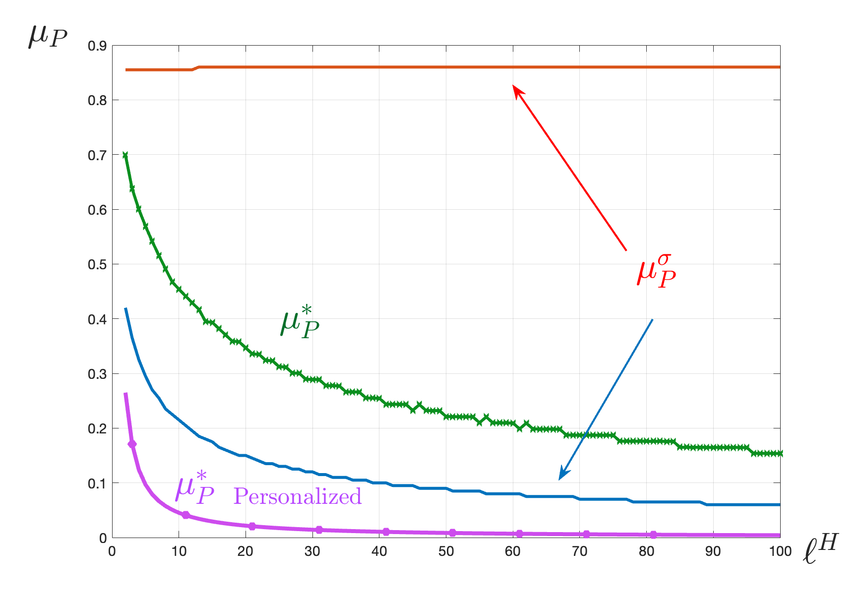
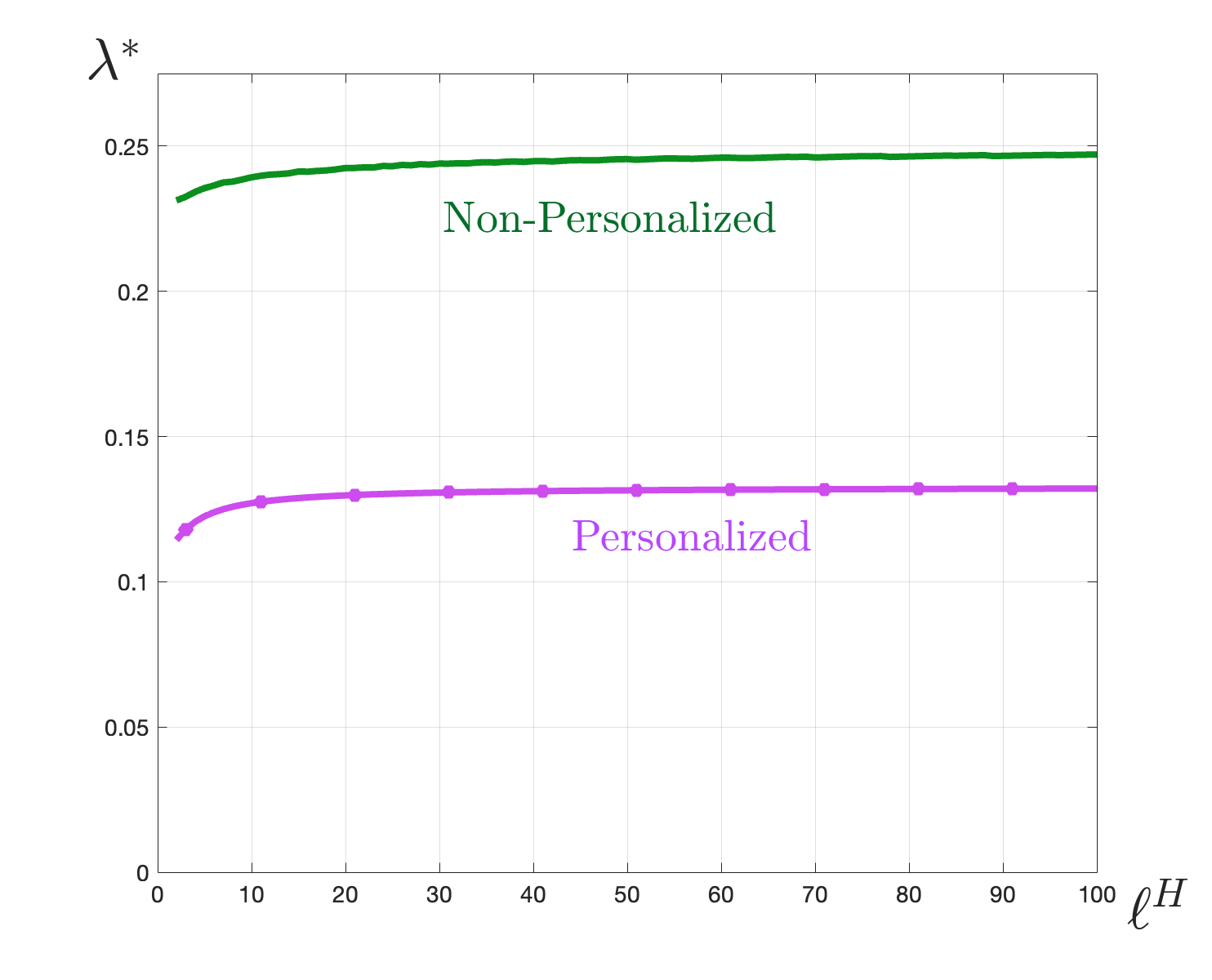
Suppose that , and . In order to compare with the personalized model of section 5, we fix at the value of 0.3 and vary and find the steady state. We assume that the fraction of high types is 0.6.
Figure 10 illustrates the idea of speed versus quality. In Figure 10a, for given likelihood ratios and , we depict the stationary level of principal’s belief (the green-crossed line) together with the beliefs that are induced in phase 2 (red and blue lines), . For comparison, we have also included the stationary belief of the principal in the personalized case for . Not surprisingly, the non-personalized stationary belief is higher – since the existence of low type agent has to be taken into account. More importantly, the beliefs induced upon transition to phase 2 are different from certainty and sometimes fairly close to highest level of uncertainty. This implies that the type that receives the exit recommendation (High type for the red line and low type for the blue line) is exiting with a low quality of information, especially when is low. In other words, in order to keep the high type engaged, low type may exit at the end of phase 1 with fairly poor information.
In Figure 10b, we depict , the rate at which phase 1 ends in the non-personalized model together with the rate of arrival of exit in the personalized model. As this figure illustrates, the speed with which transition to phase 2 happens is significantly higher in the presence of private information about beliefs.
The above discussions highlight the key differences and similarities between personalized and non-personalized communication strategies. In the personalized scenario, the principal can exert perfect control over the agent’s beliefs upon exit. In contrast, under non-personalized communication, while phase 1 of the interaction bears similarities to the personalized model, it differs in that the value of quitting from this phase is no longer zero for the principal. Furthermore, to prevent one type from quitting, it may sometimes be optimal to allow some types to leave without perfect information. Despite these distinctions, the fundamental principle governing the non-personalized optimal mechanism remains similar to that of the personalized one.
7 Extensions and Applications
In this section, we explore several extensions to our base model. We begin by incorporating random exit into our framework. We then investigate the implications of personalization on belief polarization, using our model to shed light on the ongoing debate about algorithmic news feeds and their impact on political discourse. Finally, we consider more general forms of time preferences, demonstrating how our model can accommodate various discounting structures beyond simple exponential discounting.
7.1 Random Exit
Throughout our analysis, our assumption has been that the agent can perfectly control her acquisition of information. In reality, however, attention is not perfect, and it is possible that audiences of news randomly exit. This is also in line with the extensive literature on limited attention or rational inattention that models attention as a noisy process where reducing the noise is costly; see Sims (2003) and the extensive literature following it.111111Morris and Strack (2019) provide a foundation for the static costly noise reduction model of Sims (2003) with a dynamic decision maker. Our agent essentially behaves like theirs and solves an optimal stopping problem.
To allow for random exit, suppose that if the agent is engaged at , with probability she is still engaged at . That is, she will exogenously exit in an interval with probability . Under this modification and absent any discounting by the principal, his payoff is given by
where is the decumulative probability that the principal recommends staying. In this case, unlike the baseline model, exit before can also occur exogenously and with probability . Hence, the probability has been adjusted accordingly.
The payoff of the agent is somewhat more complicated, as we need to take into account the occasions in which the agent exits exogenously and her payoff upon such exit. If the payoff of the agent upon recommended exit is , then her payoff at time conditional on being engaged is given by
When recommendation is personalized, we have which then implies that the above can be written as:
Therefore, the incentive constraint of the agent ensures that the agent’s payoff above is higher than .
The following Proposition establishes that the case with exit is similar (but not identical) to that of the unequal discounting case with :
Proposition 7.
Optimal communication with exit satisfies the following properties:
-
1.
There exists such that and for all where and satisfy
-
2.
If , then if (), () is initially revealed to the agent until where .
-
3.
If , then if (), () is initially revealed to the agent until where .
-
4.
When , and both states are revealed at a rate .
7.2 Personalization and Belief Polarization
One of the much debated issues related to political polarization is the conflict of interest between algorithmic news feeds and news consumers. The concern is that social media platforms, whose main revenue source is targeted advertising, aim to maximize engagement rather than provide the most accurate information, potentially leading to political polarization.121212The term filter bubble was coined by Pariser (2011) to describe content controlled by algorithms that can create bias.
Using an example, we demonstrate how our model can be used as a framework to study the effect of targeting news. We consider the model with random exit discussed in the previous section and compare the optimal personalized communication outcomes with those of non-personalized communication outcomes. This comparison allows us to examine the potential impacts of news targeting strategies on information dissemination.
More specifically, we assume the following parametric assumptions. The agent’s payoff as a function of her belief is , her discount rate is , and her exit rate is . Moreover, we consider two types of agents with different prior beliefs: high type and low type. We assume that their prior beliefs are , respectively, and the fraction of high types is . The prior belief of the principal is assumed to be and its discount rate to be zero.
For this specification, we compare the evolution of beliefs under personalized and non-personalized communication. In this example, the principal’s prior belief falls between those of the high and low agent types, specifically being less than the high type’s prior and greater than the low type’s prior. In the personalized case, the principal’s strategy differs for each type. For the high type, the principal initially reveals information about , as this is the state toward which the high type is more biased. Conversely, for the low type, the principal initially reveals information about , reflecting the low type’s bias. If no signals arrive, this strategy gradually shifts the agents’ beliefs toward the opposite state. The steady state points for these two types are 0.71 for the low type and 0.43 for the high type. Once the agents reach their respective steady state points, the principal reveals both states at the same rate. This process continues until either a signal arrives or the agent exits due to the exogenous exit probability.
The optimal non-personalized communication can be calculated using the arguments in Section 6. As mentioned before, there are two phases in this process. In phase 1, the principal attempts to keep both agents engaged and during this phase the beliefs merge to a steady state level. This phase continues until a transition signal arrives which results in at least one of the agents leaving. We first numerically solve the constrained optimization problem that characterizes the steady state in phase 1. Next, we guess with an initial value for first order derivative of transition signals at time zero. Using the optimality conditions and this initial guess, we can solve the rest of parameters in the model. Finally, we checked that the resulting solution satisfies the time 0 incentive constraints, if not we modify the guess and reiterate.
During phase 1, the principal’s belief changes until it converges to a steady state level, as depicted in Figure 11a. This change occurs because the transitional signal may arrive with different probabilities given the state. The principal’s belief increases from 0.55 to a long-run rate of 0.63 in phase 1. The beliefs of the two types of agents also shift, as the likelihood ratio of the beliefs remains constant.
Notes: (a) The variable is principal’s belief if phase 1 continues. Variable () is principal’s belief if the low-type (high-type) agent stays for phrase 2. (b) The variable ( is the probability that the low-type (high-type) agent stays for phase 2 (personalized phase).
The transition signal can take different forms, either instructing only one type to stay or delivering full information and allowing both types of agents to leave. Figure 11b illustrates the probability of these different outcomes. Given the parameters in this example, it is never optimal to reveal the state and let both types leave. The probabilities for which type of agent stays and which leaves vary by the arrival time of the signal, reflecting changes in beliefs. These probabilities are calculated using the concavification method mentioned in Section 6. They are associated with the arrival of one of two different types of signals that discontinuously change the principal’s and agents’ beliefs. Figure 11b also illustrates the principal’s beliefs after the arrival of each of these signals. The signal associated with the exit of the high type and the stay of the low type is indicated by the belief . After this signal arrives, the belief of the high type becomes very close to one, while the belief of the low type falls below the depicted line.131313To keep the figures tidy, we only depict the beliefs of the principal, the likelihood ratio of the beliefs stay the same, so beliefs of high type is always above the belief of principal and belief of low type is always below it. After receiving this signal, the high-type agent will quit while the low-type agent chooses to stay and gather more information and we arrive to phase 2. The opposite occurs when the signal for keeping the high type arrives.
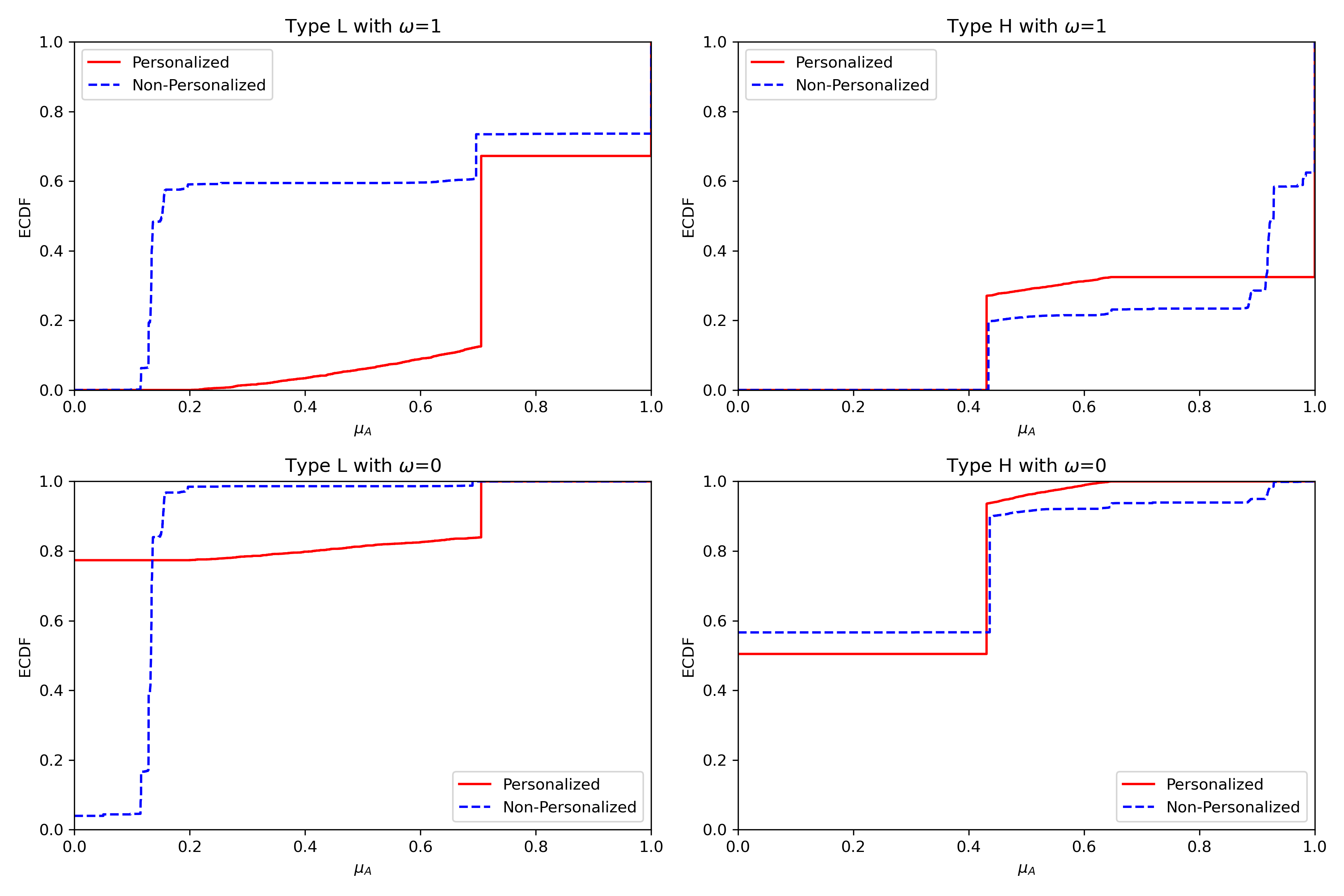
Notes: The red solid line is the empirical cumulative distribution function (CDF) of agents’ beliefs under personalized communication strategies. The blue dashed line is the empirical CDF of agents’ beliefs under non-personalized communication strategies. The left two panels are for the low-type agent and the right two panels are for the high-type agent. The upper two figures are under true state and the lower two figures are under true state . The empirical CDF comes from simulations with 10,000 belief paths for each case.
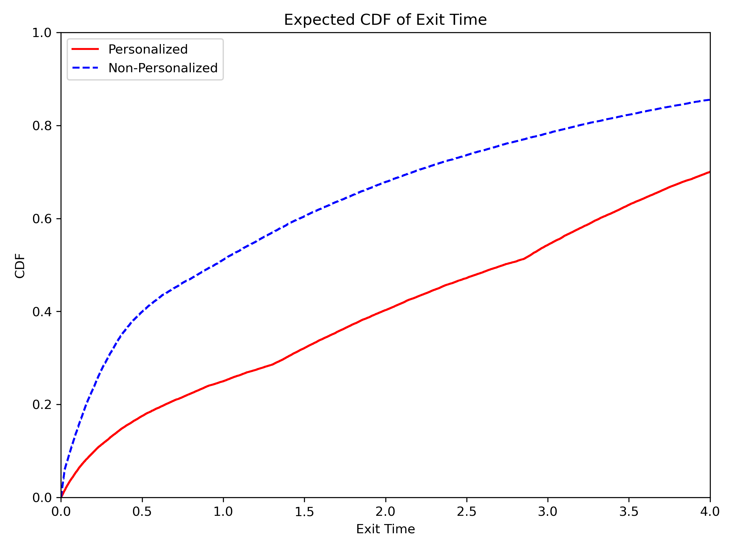
Notes: Assuming that the distribution of the true state matches the principal’s prior , the red solid line is the CDF of exit time of agents under personalized recommendation strategies, and the blue dashed line is the CDF of exit time of agents under non-personalized recommendation strategies.
Figure 12 depicts the CDF of beliefs for each state and agent type as time approaches infinity. Due to exogenous exit rates, some agents may leave without full information even in the personalized case, resulting in non-degenerate belief distributions. In the personalized case, prolonged interactions may result in agents leaving without perfect information. We observe that if the state is 1, 70% of high-type agents exit with this information compared to 30% of low-type agents, while if the state is 0, 80% of low-type agents leave with this information compared to 50% of high-type agents. This asymmetry arises from the principal catering to agents’ biases. If the true state aligns with an agent’s bias, they are likely to receive this information quickly. Otherwise, they may exit before receiving a signal revealing the opposite state and stay uninformed and biased toward the other state.
In the non-personalized case, alongside exogenous exits, the principal may choose to cater to only one agent type, prompting the other type to leave without full information. Comparing the distribution of agents across the four scenarios, we observe that in the non-personalized case, agents’ beliefs tend to be more dispersed and generally less aligned with the true state. For instance, when the state is 1, approximately 60% of low-type agents still strongly believe that the low state is likely (), and only about 25% of these agents learn that the state is actually 1. Similarly, fewer high-type agents discover that the state is 1 compared to the personalized case. These observations indicate that personalization leads to higher quality information dissemination, as agents are more likely to learn the true state under personalized communication strategies.
Another significant difference between personalized and non-personalized cases lies in the speed of information provision to agents. Figure 13 illustrates the CDF of exit times for agents in both personalized and non-personalized scenarios. We consistently observe earlier and faster exits in the non-personalized case, driven by two key forces. First, in the non-personalized case, during phase 1, the principal must keep both agent types engaged simultaneously, unable to cater to them specifically. In contrast, the personalized case allows the principal to guide each agent to a point where the cost of maintaining engagement is lowest, thus prolonging interaction. This strategy is generally not feasible when dealing with two distinct agent types simultaneously. Second, in the personalized case, the arrival of a signal leads to state revelation, increasing the reward for staying engaged. In the non-personalized case the state is not going to be perfectly revealed as it prompts both types to quit. Consequently, given the lower reward in the non-personalized scenario, the principal must increase the frequency of rewards and, therefore, the speed of information arrival. This strategy ultimately results in quicker agent exits in the non-personalized case.
These findings highlight the opposing forces present in our model, illustrating a trade-off between information quality and speed of delivery. Personalization results in slower information transmission but higher quality, while non-personalized communication leads to faster transmission but lower quality. In both scenarios, we observe that agents starting with lower priors tend to maintain their belief that their preferred state is more likely more often than those agents who initially believe the opposite state is more likely. This persistence of beliefs suggests that polarization can occur in both personalized and non-personalized communication settings. Importantly, our results indicate that personalized communication does not necessarily lead to more polarization than non-personalized communication. This insight may help explain the mixed results found in studies of the “filter bubble” phenomenon.141414Recent research offers conflicting evidence on this topic. For instance, Jones-Jang and Chung (2024) use survey data to show that social media, in contrast to traditional media, leads to less polarization. Conversely, Bakshy et al. (2015) conduct a randomized experiment and find that algorithmically ranked news feeds result in 15% lower exposure to cross-cutting content. These contrasting findings underscore the complexity of the issue and the need for further research in this area. However, it is crucial to note that a more comprehensive quantitative investigation is needed to fully understand these findings.
7.3 Other forms of Discounting
It is possible to extend our analysis to more general cases of time preferences. Specifically, suppose that principal’s preferences are given by and that of the agent is . Below, we show how this encompasses several popular models of time preferences.
7.3.1 The Nature of Time Cost for the Agent
Here, we show how different commonly used setups for inter-temporal discounting map into the setting described above:
-
1.
Exponential Discounting. The case of exponential discounting that we have so far studied is a special case of this extension. In this case the principal payoff is and the agent payoff is , where is the engagement time by the agent.We can let be the payoff of the principal and in this case the payoff of the agent is given by
whose concavity and convexity is determined by how compares to 1.
-
2.
Habit Formation a la Becker and Murphy (1988): Another example of inter-temporal preferences is the habit formation model of Becker and Murphy (1988) (also used in Allcott et al. (2022)). In this model, preferences are a function of habit – a stock variable that increases exponentially with consumption. In the context of digital addiction setting of Allcott et al. (2022), consumption can be interpreted as social media engagement. Let be the stock of habit which satisfies
and suppose that the agent’s utility is given by
When , this is equivalent to a mixed-discounting model and can similarly be expressed in terms of the payoff of the principal . As depicted in Figure 14a, when habits are weak and the agent is less patient than the principal (), MCE is decreasing over time while when when the agent is less patient than the principal, MCE is increasing over time. In the intermediate case when habits are strong enough to make , MCE initially decreases over time and as time passes habit formation becomes dominant and MCE starts increasing over time.
-
3.
A Reduced Form Model of Boredom: Another way to think about time preferences for the agent is through the lens of a reduced form version of the dual-self control model of Fudenberg and Levine (2006). We can think of the agent as consisted of two selves: a long-run planner and a short-run decider. The decider’s costly choice depends on the total time spent being engaged which can be a stock variable associated with boredom. The long-run planner in turn has to make contingent planning taking into account the cost of boredom for the short-run player. For example, the agent could have a utility of the form
where captures the cost of boredom. In this case, MCE initially increases while after a certain period it decreases. This is depicted in Figure 14b.151515See also Wojtowicz et al. (2023) for an extended version of this model with information acquisition by the dual selves.
7.3.2 Optimal Communication with General Discounting
The case of concave and convex are qualitatively the same as their associated cases with exponential discounting. Here, we describe what happens when is either a concave-convex or a convex-concave function. In these cases, perhaps not surprisingly, the solution is often determined by superimposing the Poisson gradual revelation and abrupt revelations. In what follows, we describe the nature of this superimposition and key properties of optimal revelation.
Proposition 8.
Convex-Concave Discounting. Suppose that there exists a threshold such that above is increasing for values of and decreasing for values of . Then optimal information provision has three phases:
-
1.
A phase for where only one state is revealed (towards which the agent is more optimistic) gradually, i.e. according to a time varying Poisson process. When , the evolution of beliefs is given by the ODE:
-
2.
A second phase for with where both states are gradually revealed according to a Poisson process with arrival rate .
-
3.
A final phase for with in which no information is provided and all information is revealed at .
As Proposition 8 illustrates, the convex-concave case is a superimposition of the two cases discussed before. Considering the habit formation example of section 7.3.1, when , as the agent is initially impatient relative to the principal, information must be revealed gradually and in the second phase at rate
for some . This gradual revelation is slowed down as time goes by and the agent accumulates habit. Once the force of habit formation becomes strong enough, the value of gradual revelation disappears and instead abrupt revelation is used.
8 Conclusion
This paper examines the strategic interaction between an expert (principal) seeking to maximize engagement and an agent aiming to collect information swiftly. Our analysis reveals several key insights into optimal information provision strategies in such environments.
First, we find that the relative patience of the agent and principal is a crucial determinant of the optimal information revelation strategy. In the case of common priors, a more patient agent leads to gradual information disclosure, while an impatient agent results in more abrupt revelation. This underscores the importance of considering time preferences in designing engagement strategies.
Second, our model demonstrates that when the principal and agent have different prior beliefs, optimal disclosure often involves “catering to the bias.” The principal tends to initially reveal information aligned with the agent’s bias, exploiting this asymmetry to prolong engagement. This finding has significant implications for understanding how information providers may strategically utilize belief disagreements.
Third, in scenarios with private agent beliefs, we identify two phases in communication strategies. During phase 1, the principal attempts to keep both agent types engaged. A transition signal during this phase determines which type of agent should stay and which should leave. Notably, the principal may allow one agent to depart without full information, contrasting with the personalized case, to keep the other agent engaged. Once only one agent type remains, the strategy reverts to the personalized case.
Our comparison of personalized and non-personalized information revelation strategies highlights important trade-offs. Personalization enables longer engagement and slower information delivery, while non-personalized approaches lead to faster information transmission but may result in lower quality information overall.
References
- Acemoglu and Johnson (2024) Acemoglu, D. and S. Johnson (2024): “The Urgent Need to Tax Digital Advertising,” Network Law Review, Spring.
- Allcott et al. (2020) Allcott, H., L. Braghieri, S. Eichmeyer, and M. Gentzkow (2020): “The Welfare Effects of Social Media,” American Economic Review, 110, 629–76.
- Allcott et al. (2022) Allcott, H., M. Gentzkow, and L. Song (2022): “Digital addiction,” American Economic Review, 112, 2424–2463.
- Aumann (1976) Aumann, R. J. (1976): “Agreeing to Disagree,” The Annals of Statistics, 4, 1236–1239.
- Bakshy et al. (2015) Bakshy, E., S. Messing, and L. A. Adamic (2015): “Exposure to ideologically diverse news and opinion on Facebook,” Science, 348, 1130–1132.
- Ball and Knoepfle (2023) Ball, I. and J. Knoepfle (2023): “Should the timing of inspections be predictable?” Available at SSRN 4419716.
- Becker and Murphy (1988) Becker, G. S. and K. M. Murphy (1988): “A Theory of Rational Addiction,” Journal of Political Economy, 96, 675–700.
- Che et al. (2023) Che, Y.-K., K. Kim, and K. Mierendorff (2023): “Keeping the Listener Engaged: a Dynamic Model of Bayesian Persuasion,” Journal of Political Economy, 131, null.
- DeJarnette et al. (2020) DeJarnette, P., D. Dillenberger, D. Gottlieb, and P. Ortoleva (2020): “Time lotteries and stochastic impatience,” Econometrica, 88, 619–656.
- Doval and Skreta (2024) Doval, L. and V. Skreta (2024): “Constrained information design,” Mathematics of Operations Research, 49, 78–106.
- Dunford and Schwartz (1988) Dunford, N. and J. T. Schwartz (1988): Linear operators, part 1: general theory, vol. 10, John Wiley & Sons.
- Dworczak and Martini (2019) Dworczak, P. and G. Martini (2019): “The simple economics of optimal persuasion,” Journal of Political Economy, 127, 1993–2048.
- Ely (2017) Ely, J. C. (2017): “Beeps,” American Economic Review, 107, 31–53.
- Ely and Szydlowski (2020) Ely, J. C. and M. Szydlowski (2020): “Moving the Goalposts,” Journal of Political Economy, 128, 468–506.
- Fudenberg and Levine (2006) Fudenberg, D. and D. K. Levine (2006): “A Dual-Self Model of Impulse Control,” American Economic Review, 96, 1449–1476.
- Guo (2016) Guo, Y. (2016): “Dynamic delegation of experimentation,” American Economic Review, 106, 1969–2008.
- Hadfield (2007) Hadfield, G. K. (2007): “Legal barriers to innovation: The growing economic cost of professional control over corporate legal markets,” Stan. L. Rev., 60, 1689.
- Hadfield (2022) ——— (2022): “Legal markets,” Journal of Economic Literature, 60, 1264–1315.
- Halac et al. (2016) Halac, M., N. Kartik, and Q. Liu (2016): “Optimal contracts for experimentation,” The Review of Economic Studies, 83, 1040–1091.
- Hébert and Zhong (2022) Hébert, B. and W. Zhong (2022): “Engagement Maximization,” .
- Henry and Ottaviani (2019) Henry, E. and M. Ottaviani (2019): “Research and the approval process: The organization of persuasion,” American Economic Review, 109, 911–955.
- Hiriart-Urruty and Lemaréchal (2004) Hiriart-Urruty, J.-B. and C. Lemaréchal (2004): Fundamentals of convex analysis, New York: Springer.
- Jones-Jang and Chung (2024) Jones-Jang, S. M. and M. Chung (2024): “Can we blame social media for polarization? Counter-evidence against filter bubble claims during the COVID-19 pandemic,” New Media & Society, 26, 3370–3389.
- Kamenica and Gentzkow (2010) Kamenica, E. and M. Gentzkow (2010): “Bayesian persuasion: Web appendix,” American Economic Review.
- Kamenica and Gentzkow (2011) ——— (2011): “Bayesian Persuasion,” American Economic Review, 101, 2590–2615.
- Keller and Rady (2010) Keller, G. and S. Rady (2010): “Strategic Experimentation with Poisson Bandits,” Theoretical Economics, 5, 275–311.
- Keller et al. (2005) Keller, G., S. Rady, and M. Cripps (2005): “Strategic experimentation with exponential bandits,” Econometrica, 73, 39–68.
- Kleiner et al. (2021) Kleiner, A., B. Moldovanu, and P. Strack (2021): “Extreme Points and Majorization: Economic Applications,” Econometrica, 89, 1557–1593.
- Knoepfle (2020) Knoepfle, J. (2020): “Dynamic Competition for Attention,” Tech. rep., University of Bonn and University of Mannheim, Germany.
- Koh and Sanguanmoo (2022) Koh, A. and S. Sanguanmoo (2022): “Attention capture,” arXiv preprint arXiv:2209.05570.
- Koh et al. (2024) Koh, A., S. Sanguanmoo, and W. Zhong (2024): “Persuasion and Optimal Stopping,” arXiv preprint arXiv:2406.12278.
- Levy (2021) Levy, R. (2021): “Social Media, News Consumption, and Polarization: Evidence from a Field Experiment,” American Economic Review, 111, 831–70.
- Luenberger (1997) Luenberger, D. G. (1997): Optimization by Vector Space Methods, John Wiley & Sons.
- Morris and Strack (2019) Morris, S. and P. Strack (2019): “The wald problem and the relation of sequential sampling and ex-ante information costs,” Available at SSRN 2991567.
- Orlov et al. (2020) Orlov, D., A. Skrzypacz, and P. Zryumov (2020): “Persuading the Principal to Wait,” Journal of Political Economy, 128, 2542–2578.
- Pariser (2011) Pariser, E. (2011): The filter bubble: What the Internet is hiding from you, penguin UK.
- Renault et al. (2017) Renault, J., E. Solan, and N. Vieille (2017): “Optimal dynamic information provision,” Games and Economic Behavior, 104, 329–349.
- Saeedi and Shourideh (2023) Saeedi, M. and A. Shourideh (2023): “Optimal Rating Design,” Working Paper.
- Sims (2003) Sims, C. A. (2003): “Implications of rational inattention,” Journal of monetary Economics, 50, 665–690.
- Smolin (2021) Smolin, A. (2021): “Dynamic Evaluation Design,” American Economic Journal: Microeconomics, 13, 300–331.
- Strömberg (2004) Strömberg, D. (2004): “Mass media competition, political competition, and public policy,” The Review of Economic Studies, 71, 265–284.
- Strulovici (2010) Strulovici, B. (2010): “Learning while voting: Determinants of collective experimentation,” Econometrica, 78, 933–971.
- Wang et al. (2021) Wang, X., J. Shi, and H. Kong (2021): “Online Health Information Seeking: A Review and Meta-Analysis,” Health Communication, 36, 1163–1175, pMID: 32290679.
- Wojtowicz et al. (2023) Wojtowicz, Z., N. Chater, and G. Loewenstein (2023): “Boredom and Flow: An Opportunity Cost Theory of Attention-Directing Motivational States,” Available at SSRN 3339123.
Appendix A Proofs
A.1 Proof of Theorem 1
Proof.
We prove a more general version of the theorem. As we discussed in Section 7.3.2, our model is equivalent to one in which time is given by with and the payoff of the principal is given by while the payoff of the agent is given by
where is a strictly decreasing and positive function with possibly satisfying . Note that when exponential discounting, and with .
For completeness and easier reference, let us restate Theorem 1 on page 217 of Luenberger (1997):
Theorem 2.
Let be a linear vector space, a normed space, a convex subset of , and a positive cone in . Suppose that contains an interior point. Let be a real-valued convex functional on and a convex mapping from into . Assume the existence of for which , i.e., is an interior point of . Let
| (12) |
and assume is finite. Then there is an element in such that
| (13) |
Furthermore, if the infimum is achieved in (12) by an , it is achieved by in (13) and
We will verify that our optimization problem satisfies the conditions in Theorem 2.
A key assumption in Theorem 2 is the existence of ; existence of . This proves difficult in general. Therefore, we consider two cases: 1. when and 2. when . In the first case, we can use Theorem 2, and in the second case, we use a limiting argument.
Case 1. Suppose that . We define the objects in Theorem 2 as follows:
where in the above is the set of real numbers that are non-negative. Trivially, and satisfy the hypothesis in Theorem 2. The set is a convex set, and is a convex cone. Finally, since is a convex function,
which then implies that
In other words, the function is convex. As a result, the function is convex.
Let where
and the strict concavity of implies that if , the above is positive. Let be the associated member of . We have that:
If we let , then we have that
and therefore, a ball of radius around is a subset of . Moreover, is linear in and its value is bounded below by 0 and above by . Finally, since the functions are bounded, the set of ’s such that is compact. This means that the optimization achieves its value, and this confirms all the hypotheses of Theorem 2.
By standard Representation Theorems (Riesz-Kakutani-Markov), see Theorem IV.16 in Dunford and Schwartz (1988) as an example, the dual of the space of bounded functions is isomorphic to the space of finitely additive measures of bounded variation or in turn the space of functions of bounded variations that vanish at . This implies that there must exists where , is an increasing function of bounded variation161616The fact that must be (weakly) increasing is implied by which means that , the dual of the cone which is defined as members of , such that for all . with such that is the solution to if
Note that is the set of positive, bounded, and non-increasing functions. Thus, it is a convex cone in . Hence, we can apply the following Lemma from Luenberger (1997) – Lemma 1, page 227, section 8.7:
Lemma 4.
Let be a Fréchet differentiable convex functional on a real normed space . Let be a convex cone in . A necessary and sufficient condition for to minimize over is that
Applying the above to , we have
| (14) | ||||
| (15) |
where in the above is an arbitrary member of and is the belief of the agent given by calculated at the optimum. This proves the claim for case 1.
To show the result for case 2, i.e., , we use continuity arguments. Since , we can apply the above logic to with . We then consider the solution and its associated multiplier that satisfy the above condition. We extend to the entire interval by setting . We use the following lemma to characterize the properties of a limit point of the solutions and multipliers .
Lemma 5.
There exists a constant such that for all values of , .
We relegate the proof to Section A.7.
Since each function is increasing, Lemma 5 together with the compactness of bounded functions in the space of functions with bounded variations171717By the Banach-Alaoglu theorem. imply that there exists a bounded function with bounded variation and a subsequence of ’s, given by’s, so that
| (16) |
Moreover, since each is increasing so is .
Additionally, note that , . This implies that the measure associated with the function , i.e., is the CDF of , is a finite measure. This implies that for all functions with bounded derivatives.
Since ’s are bounded, they must converge as . By Berge’s maximum theorem, the limit of should be an optimizer for . The result then follows from the continuity of the expressions in (14). ∎
A.2 Proof of Proposition 1
Proof.
We use Theorem 1 and construct multiplier so that abrupt revelation is optimal.
where
Under abrupt revelation, the distribution of exit rates are
As we show in the proof of Theorem 1, is equivalent to
which is satisfied by construction.
Next, we need to show that for all non-increasing positive functions , is satisfied. We have
The above is linear in . Thus, if we show that for any positive and decreasing function , and , this proves the desired result. We will show that ; the second inequality can be shown similarly. We have
where the above is negative since and . Finally, we should note that satisfies the complementary slackness condition as for all and the incentive constraint is slack, while and the incentive constraint is binding. This concludes the proof. ∎
A.3 Proof of Proposition 2
Proof.
For the proof, we will focus on the case. The proof for the case with is almost identical. Let be the solution to the following differential equation:
with initial value given by . This differential equation is derived from the binding incentive constraint 3 using the fact that in the first phase. Simple calculations allow us to show that the solution of the above satisfies
and thus exists, and it is unique and decreasing. Moreover, we can define as the first time that given by
We extend beyond by setting it equal to . In addition, the function defines the engagement probability functions given by
where . The variable is the arrival rate of revelation in the second phase and is calculated using the 3. Additionally, for all values of , let be defined by
where . This is a simple ordinary differential equation whose solution is given by
| (17) | ||||
Finally, we set
where exists because for large values of , and .
We can rewrite the derivative of the Lagrangian using integration by part as:
where in the above . Since for all which implies that for all values of . We can thus write
In the above, the inequality follows from two observations: first, since is non-increasing, it must be that ; second, which then implies that and as we will show later .
To finish the proof, we need to show that . To see these, recall from (17) that
where in the above, we have used the definition of and the fact that as , . Finally,
where the inequality follows from the fact that for all values of . This concludes the proof. ∎
A.4 Proof of Proposition 3
Proof.
As in the statement of the Proposition, we focus on ; the case with is the mirror of this case. To prove the claim of the proposition, we first define a class of exit probability functions parametrized by – the agent’s belief at the end of phase 1. Given , the length of phase 1, , and end of engagement, as well as the agent’s belief is given by
| (18) | ||||
When the length of phase 1 is 0 while its maximum length is when . These beliefs are associated with engagement probability functions given by
For each parameter value , we also define the following Lagrange multipliers given by
and for values of the ODE
| (19) |
holds where and finally, we set for values of . Let be the value of the parameter such that either the above multiplier satisfies and if such value does not exist, we set . Later, we will show that there exists at most one such value of and that has to hold. In other words, if , we will show that . Let and be the associated end of phase 1 and phase 2. Finally, we define as
For this allocation, we show that and for all non-increasing and positive pair of functions . Moreover, the multipliers need to satisfy the complementary slackness and has to be non-decreasing.
-
1.
Complementary Slackness (CS): The incentive constraint is binding when and when . Since is flat for , for CS to be satisfied, we need to be positive. which holds, and to be increasing when . The ODE in 19 has an exact solution given by
(20) Differentiating , we have
Since for all values of , the above implies that if , then for all values of , . At we have
Since , we must have that and hence .
Additionally, we have to show that . We haveThe first expression above is positive since and the second expression is positive since is convex and positive. Therefore, . Additionally,
The first two terms in the above expression are positive since . Additionally, since satisfies the ODE (19), we can write the integrand in the last integral as
(21) In the above, since , , and , is positive and increasing. If , then which implies that the above is positive. Finally, when ,
As a result, is increasing, and therefore the integrand in (21) is decreasing in . Its value at is given by
By construction of , we must have that . Since the integrand in (21) is decreasing in , it must always be positive. As a result, the last integral in the expression for is positive and .
-
2.
Optimality Condition (14): Since is linear in , it is sufficient to show for and with an arbitrary non-increasing and non-negative function. For such values, we have
Given our construction of the allocation and the multipliers, we can rewrite the above as
where the last inequality follows from and .
Similarly, for , we can writeSince , the last integral is negative. It is thus sufficient to show that the first two terms add up to a negative value. We can use integration by parts to write
Earlier we have shown that , see the discussion following (21). Hence, since , that is, is decreasing, the above integral is negative, which is the desired result.
-
3.
Optimality Condition (15): In the proof of Theorem 1, we showed that Equation (15) boils down to checking . Given the values of and , we have
Since , we can use the above to write
Recall the definition of which implies that and hence, we can write the above as
Now, given that satisfies the ODE (19), we can multiply the ODE by and integrate over time. The resulting expression is 0 and thus can be added to the above. Hence,
Using integration by part the above simplifies to:
Finally, to finish the proof, we will show that there is at most one for which holds and that if such exist it must be less than 1. To see this, suppose that . In this case, . Note under this assumption, engagement strategy in phase 2 does not exist and hence we must have that . Since , this is less than which implies that if exists, it cannot be equal to 1. In order to show the existence of , we will show that as we increase , decreases. As a result, either there is a unique value under which or that for all values of , in which case . To avoid further lengthening the proof of this proposition, we show this in the proof of Corollary 1 below. ∎
A.5 Proof of Corollary 1
Proof.
We first focus on the case with or . In this case, we first show that is strictly decreasing in . As a result, to have no phase 1, we would need for . For a given , since is strictly increasing over phase 2, we can do a change of variable and write the Lagrange multiplier as a function of beliefs so that . The law of motion for in phase 2 can be written as:
This implies that
Given the above, we have
We can use this change of variable and write the solution for in (20) as
Using the definition of , we can rewrite the above as
Hence,
Taking a derivative of the above with respect to , we have
Hence, either there exists a unique such that or that
in which case and phase 1 is of length 0. That is
or
| (22) |
The derivative of the above with respect to is
Additionally an increase in decreases . This implies that the inequality (22) holds for low values of .
When or , the law of motion for in phase 2 can be written as
This implies that
Given the above, we have
At the same time, the ODE characterizing the Lagrange multiplier in phase 2 is given by
with . In this case, the solution of this ODE is given by
We can use a change of variable as above and write
A similar argument as before establishes that is increasing in and thus for phase 1 to be of length 0, we need
A similar argument as before shows that the LHS of the above is decreasing in and thus holds for high enough values of and thus establishing the result. ∎
A.6 Proof of Proposition 4
Proof.
We start by characterization of the steady-state level, i.e., where satisfies (6). Given its definition in (6), when , then, or while when , then or . Moreover, since and , we have
Moreover, when and , we must have
Since and , for , the above is positive. Moreover, if and , then
Therefore, when , is strictly increasing in .
Let be defined by
This is the incentive constraint of the agent when
In line with the rest of the analysis, we assume that . The Lagrange multiplier is defined by
Given the definition of and the property mentioned above, and have the same sign, which implies that , and . Given the above definition, satisfies
where in the above we have used the definition of from (6). Similarly, we can show that
A simple examination of the above illustrates that they are the First Order Condition of the Lagrangian with respect to and . This establishes the optimality of the steady state mentioned above.
In order to prove the claim of the Proposition, we will show the case where . The other case is the mirror of this proof. Suppose that satisfies the differential equation (7) in phase 1 until it reaches the value which is defined by
Such a value of is uniquely determined since the above becomes
| (23) |
whenever . Since the numerator is decreasing in and the denominator is increasing, the above have at most one solution. When no such exist, we set . We let be the time by which this value of belief is reached. Additionally, let be the associated engagement policy given by
Given this, the rest of the proof is very similar to that of Proposition 2. We construct the Lagrange multiplier using the ODE
for a given value of . For values of , we set
where has to satisfy
Since LHS is positive, that solves the above is also positive. Finally, the Lagrange multipliers are constructed according to:
where . The FOC with respect to is satisfied when or when , given that satisfies the above ODE. To show optimality, it is sufficient to show that
We prove the stronger result that for all
| (24) |
To establish this inequality, we realize that , and since is the lowest time for which , it must be that for all values of , .
Recall that satisfies the following
Let . We can use the ODE governing and rewrite the LHS of (24) as
We can divide the above by and rewrite the resulting expression as
In order to show that the above is positive, we will show that it is decreasing and its value at is positive. Its derivative with respect to is given by
| (25) |
We show that each of the expressions above are negative. To do so, note that for all values of , we must have that , given the definition of . Therefore
which is proportional to the last expression in (25). Moreover, since and are increasing, and is decreasing, we must have that . Finally,
This implies that (25) is negative. Thus, it is sufficient to show that (24) holds at and this automatically holds given that at , and which implies that at , (24) holds with equality. This concludes the proof. ∎
A.7 Proof of Lemma 5
Proof.
First, we note that we can consider and its associated solution
. Let to be the infimum value such that and if such value does not exist, we set . We note that we must have . Suppose that , then we must have that for all . Hence, the incentive constraint is given by
Since and , the only way the above constraint can hold is if . This implies that . Using a similar argument, we have that . Note that since the marginal benefit of is always 1, we can assume that that for all .
Next, let us consider where . We can then write the relations in (14) as
By sending , the above becomes
| (26) | |||
Similarly, we can consider and do the same as above. This would then imply that the LHS of (26) is non-negative and thus has to be 0. If we let , then we can write the above as
| (27) |
Repeating the above for , we arrive at
| (28) |
A property of the functions are
Convexity of implies that
Which further implies that
Now, we consider (27) and (28) and take equally weighted average and use the above inequality to arrive at
Using integration by parts, we can write
where in the above we have used the fact that . We then have that
Hence, in order to prove the claim, it is sufficient to show that the right hand side stays bounded as converges to .
We know that and thus it is bounded above. Moreover, since , we can use complementary slackness to write as
The RHS of the above is less than which then implies that and stay bounded below . Finally, plugging in into (14) and subtract (15) we arrive at
which implies that is also bounded. This concludes the proof. ∎