The Basic Theory of Clifford-Bianchi Groups for Hyperbolic $n$-Space

Abstract

Let $K$ be a $\mathbb{Q}$-Clifford algebra associated to an $(n-1)$-ary positive definite quadratic form and let $\mathcal{O}$ be a maximal order in $K$. A Clifford-Bianchi group is a group of the form $\operatorname{SL}_{2}(\mathcal{O})$ with $\mathcal{O}$ as above. The present paper is about the actions of $\operatorname{SL}_{2}(\mathcal{O})$ acting on hyperbolic space $\mathcal{H}^{n+1}$ via Möbius transformations $x\mapsto(ax+b)(cx+d)^{-1}$.

We develop the general theory of orders exhibiting explicit orders in low dimensions of interest. These include, for example, higher-dimensional analogs of the Hurwitz order. We develop the abstract and computational theory for determining their fundamental domains and generators and relations (higher-dimensional Bianchi-Humbert Theory). We make connections to the classical literature on symmetric spaces and arithmetic groups and provide a proof that these groups are $\mathbb{Z}$-points of a $\mathbb{Z}$-group scheme and are arithmetic subgroups of $\operatorname{SO}_{1,n+1}(\mathbb{R})^{\circ}$ with their Möbius action.

We report on our findings concerning certain Clifford-Bianchi groups acting on $\mathcal{H}^{4}$, $\mathcal{H}^{5}$, and $\mathcal{H}^{6}$ .

1 Introduction

We introduce Clifford-Bianchi groups $\operatorname{SL}_{2}(\mathcal{O})$ for $\mathcal{O}$, an order in a Clifford algebra $\operatorname{Clf}(q)$ associated to a positive definite integral quadratic $(n-1)$-form $q$ (general background on Clifford algebras is given in §2). These groups act on hyperbolic $(n+1)$-space $\mathcal{H}^{n+1}$ and simultaneously generalize the modular group action on hyperbolic $2$-space and Bianchi group actions on hyperbolic $3$-space to all dimensions.

In what follows, when $q=d_{1}^{2}y_{1}^{2}+d_{2}y_{2}^{2}+\cdots+d_{m}y_{m}^{2}$ over a commutative ring $R$ we use Hilbert symbol notation

$$\operatorname{Clf}(q)=\left(\frac{-d_{1},-d_{2},\ldots,-d_{m}}{R}\right)$$

for the associated Clifford algebra. Typically, $R$ will be $\mathbb{R},\mathbb{Q}$, or $\mathbb{Z}$, and the $d_{i}$ will be a coprime collection of squarefree positive integers so that $q$ is a primitive quadratic form in the sense of [Knus1991, p. 164].

1.1 Main Results

We postpone definitions in order to expeditiously state results. In what follows, $\mathbb{C}_{n}=\mathbb{R}[i_{1},\ldots,i_{n-1}]$ is the associative algebra of Clifford numbers of $\mathbb{R}$-vector space dimension $2^{n-1}$ and $V_{n}\subset\mathbb{C}_{n}$ is the $n$-dimensional $\mathbb{R}$-vector subspace of Clifford vectors generated by $i_{0}=1,i_{1},\ldots,i_{n-1}$.

Theorem 1.1.1 (§5.4).

There exists a uniformization of hyperbolic $n$-space within the Clifford vectors of the Clifford numbers $\mathcal{H}^{n+1}\subset V_{n+1}$ such that there exists an action of $\operatorname{PSL}_{2}(\mathbb{C}_{n})$ given by

$$x\mapsto(ax+b)(cx+d)^{-1}.$$

This action gives an isomorphism $\operatorname{PSL}_{2}(\mathbb{C}_{n})\cong\operatorname{Isom}(\mathcal{H}^{n+1})^{\circ}$ where $\operatorname{Isom}(\mathcal{H}^{n+1})^{\circ}$ is the connected component of the isometry group of the Riemannian manifold $\mathcal{H}^{n+1}$.

Correcting some work of McInroy [McInroy2016] and developing a theory of Weil restriction for Clifford algebras (§4.1), we prove the following.

Theorem 1.1.2 (§4.1).

1. There exists a $\mathbb{Z}$-ring scheme $\operatorname{Clf}_{q}$ such that for every commutative ring $R$ we have

   $$\operatorname{Clf}_{q}(R)=\operatorname{Clf}(q_{R}),$$

   where $q_{R}$ is the quadratic form base changed to $R$.

2. There exists a $\mathbb{Z}$-group scheme $\operatorname{SL}_{2}(\operatorname{Clf}_{q})$ such that for every commutative ring $R$ we have

   $$\operatorname{SL}_{2}(\operatorname{Clf}_{q})(R)=\operatorname{SL}_{2}(\operatorname{Clf}(q_{R})).$$

Using an arithmetic version of Bott periodicity (§2.11) and painstakingly checking various conjugation and normalization conventions across the literature, we are able to make the following arithmetic connection to Spin groups generalizing and spreading out the classical relationship between $\operatorname{SL}_{2}(\mathbb{C})$ and the Lorentz group.

Theorem 1.1.3 (§4.2).

For every positive definite integral quadratic $(n-1)$-form $q$ there exists an $n+2$-form $Q$, which is a $\mathbb{Z}$-form of the real quadratic form of signature $(1,n+1)$, such that $\operatorname{SL}_{2}(\operatorname{Clf}_{q})\cong\operatorname{Spin}_{Q}$ as $\mathbb{Z}$-group schemes. In particular, we have

$$\operatorname{SL}_{2}(\mathbb{C}_{n})\cong\operatorname{SL}_{2}(\operatorname{Clf}_{q})(\mathbb{R})\cong\operatorname{Spin}_{Q}(\mathbb{R})\cong\operatorname{Spin}_{1,n+1}(\mathbb{R}).$$

Throughout this paper we need to assume that our orders are closed under the transpose/reversal involution $*$ of Clifford algebras (§2.1). Using theorems of Bass and spin exact sequences of $\mathbb{Z}$-group schemes, we prove the following.

Theorem 1.1.4 (§6).

For $\mathcal{O}$ an order in $\left(\frac{-d_{1},-d_{2},\ldots,-d_{n-1}}{\mathbb{Q}}\right)$, the groups $\operatorname{PSL}_{2}(\mathcal{O})$ are arithmetic. More precisely, $\operatorname{PSL}_{2}(\mathcal{O})$ can be identified with an arithmetic subgroup of $\operatorname{SO}_{1,n+1}(\mathbb{R})^{\circ}$ acting on $\mathcal{H}^{n+1}$, and the action is given by Möbius transformations.

As a consequence the group $\Gamma=\operatorname{PSL}_{2}(\mathcal{O})$ acts discretely and with finite covolume.

This addresses an issue stated, for example, in Asher Auel’s thesis about the prime $p=2$ in the étale topology (Remark 1.5.1), and clarifies previous work [Elstrodt1988, Maclachlan1989]. (The issue with $p=2$ is why we need to work with the fppf topology and not the étale topology.)

Discreteness and finite covolume follow from an application of the Borel–Harish-Chandra Theorem (§6.2). We note that we are very careful with integrality issues and never take $\mathbb{Z}$-points of $\mathbb{Q}$-group schemes in this paper.

For each of these groups $\Gamma=\operatorname{SL}_{2}(\mathcal{O})$ acting on $\mathcal{H}^{n+1}$ there exist orbifolds $\mathcal{Y}(\Gamma)$ analogous to Bianchi and modular curves (§5.6). If $K$ is the rational Clifford algebra of $\mathcal{O}$ and $\operatorname{Vec}(K)$ is the set of Clifford vectors, we define the partial Satake compactification of $\mathcal{H}^{n+1}$ to be

$$\mathcal{H}^{n+1}\cup\operatorname{Vec}(K)\cup\{\infty\}.$$

The elements $\operatorname{Vec}(K)\cup\{\infty\}$ are called the cusps. We also have compactified quotients $\mathcal{X}(\Gamma)$ (§5.6).

Using the isomorphism $\operatorname{SL}_{2}(\operatorname{Clf}_{q})\cong\operatorname{Spin}_{Q}$, we can use a result of Satake to prove that our locally symmetric space parametrizes abelian varieties with “even Clifford multiplication”, giving a generalization of the theory of Shimura curves.

Theorem 1.1.5 (§5.7).

Let $\Gamma=\operatorname{PSL}_{2}(\mathcal{O})$, for $\mathcal{O}$ an order in the Clifford algebra associated to a positive definite integral quadratic $(n-1)$-form. The orbifolds $\mathcal{Y}(\Gamma)=[\Gamma\backslash\mathcal{H}^{n+1}]$ (with a choice of auxiliary data) parametrize abelian varieties of dimension $2^{n}$ with $\mathcal{O}_{+}$-multiplication, where $\mathcal{O}_{+}$ is the the even subalgebra of $\mathcal{O}$.

Given such a rich and interesting theory, it is natural to want to find examples.

Result 1.1.6 (§3.1).

We give an algorithm for computing maximal orders $\mathcal{O}$ containing $\left(\frac{-d_{1},-d_{2},\ldots,-d_{n-1}}{\mathbb{Z}}\right)$ up to Clifford conjugacy.

The algorithm finds $p$-maximal orders using discriminant considerations and intersects them to find maximal orders.

To explain our classification of orders in low-dimensional examples, we start by recalling some orders most algebraic number theorists are familiar with. In $\mathbb{Q}[i]=\left(\frac{-1}{\mathbb{Q}}\right)$ there exists a unique maximal order $\mathcal{O}_{2}=\mathbb{Z}[i]$, namely the Gaussian integers. In $\mathbb{Q}[i,j]=\left(\frac{-1,-1}{\mathbb{Q}}\right)$ there exists a unique maximal order $\mathcal{O}_{3}$, called the Hurwitz order, containing $\left(\frac{-1,-1}{\mathbb{Z}}\right)$, which is called the Lipschitz order. In $\mathbb{Q}[\sqrt{3}i]=\left(\frac{-3}{\mathbb{Q}}\right)$ there exists a unique maximal order called the Eisenstein integers. The Gaussian integers, the Hurwitz order, and the Eisenstein integers are known to be Euclidean domains.

Result 1.1.7 (§3.4).

In higher dimensions we develop a theory of Clifford-Euclidean domains and greatest common divisor algorithms.

Using our algorithm and our theory of Clifford-Euclidean algorithms, we do some classification of orders in low dimensions. These are reviewed in more detail in §1.3.

Theorem 1.1.8.

1. In $\left(\frac{-1,-1,-1}{\mathbb{Q}}\right)$ there exists a unique maximal order $\mathcal{O}_{4}$ containing $\left(\frac{-1,-1,-1}{\mathbb{Z}}\right)$. Furthermore, the order is Clifford-Euclidean and its Clifford vectors form a $D_{4}$ root lattice. Also, the triality automorphism is witnessed by a higher-dimensional analog of “complex multiplication” for these lattices. The order $\left(\frac{-1,-1,-1}{\mathbb{Z}}\right)$ is neither Clifford-Euclidean nor cuspidally principal.

2. In $\left(\frac{-1,-1,-1,-1}{\mathbb{Q}}\right)$ there are two Clifford conjugacy classes of orders containing $\left(\frac{-1,-1,-1,-1}{\mathbb{Z}}\right)$: one class corresponding to the five $[5,4,1]$ doubly even binary codes, and one corresponding to the trivial code in $\mathbb{F}_{2}^{5}$.

3. In $\left(\frac{-1,-3}{\mathbb{Q}}\right)$ there exist two Clifford conjugacy classes of orders containing $\left(\frac{-1,-3}{\mathbb{Z}}\right)$. All of these orders are Clifford-Euclidean.

4. In $\left(\frac{-1,-1,-3}{\mathbb{Q}}\right)$ there exist two Clifford conjugacy classes of order containing $\left(\frac{-1,-1,-3}{\mathbb{Z}}\right)$.

We also found a number of other exotic orders in our investigations.

Theorem 1.1.9.

There is an order $\mathcal{O}_{E_{8}}\subset\left(\frac{-1,-1,-1,-1,-1,-1,-1}{\mathbb{Q}}\right)$ whose Clifford vectors are an $E_{8}$ root lattice. The group $\operatorname{PSL}_{2}(\mathcal{O}_{E_{8}})$ acts on $\mathcal{H}^{9}$.

We present some questions and conjectures about higher-dimensional examples and connections to doubly even codes (§1.3, §3.6).

As expected, we can say something about Clifford-Euclideanity and cuspidal principality.

Theorem 1.1.10 (§7.5).

If $\mathcal{O}\subset K$ is Clifford-Euclidean then there is a single orbit of a cusp. In general there is only an injection from orbits of cusps into the (left) ideal class set of $\mathcal{O}$.

Note that in particular we provide examples which are not cuspidally principal and hence whose $\mathcal{X}(\Gamma)$ has more than one cusp.

For computing the fundamental domains we need to generalize some theoretical work of Swan [Swan1971] and develop a Bianchi-Humbert reduction theory which establishes a bijection between $\mathcal{H}^{n+1}$ and classes of positive definite Clifford-Hermitian forms (§7). Using this description we give a “proof by moduli” which shows that Clifford-Hermitian forms in an orbit with minimal unimodular value at $(1,0)$ are those which are in the fundamental domain (§7.9).

Result 1.1.11 (§3.2).

We give an algorithm for computing generators for the Clifford group $\mathcal{O}^{\times}$ for these orders. Furthermore, we give an algorithm for computing the fundamental domain for $\operatorname{SL}_{2}(\mathcal{O})_{\infty}=\operatorname{Stab}_{\operatorname{SL}_{2}(\mathcal{O})}(\infty)$ acting on $V_{n}$.

It turns out that the stabilizers of $\infty$ for these Clifford-Bianchi groups have a very rich geometry; for example, the fundamental domain for $\Gamma_{\infty}=\operatorname{PSL}_{2}(\mathcal{O}_{4})_{\infty}$ is 4 copies of the 24-cell (octaplex) glued together.

Result 1.1.12 (§9.3).

We give an algorithm for computing the boundary bubbles of the fundamental domain.

This algorithm uses linear programming and dynamically introduces bubbles. This, together with the previous result, gives an algorithm for computing the fundamental domain.

Result 1.1.13.

If $\mathcal{O}$ is Clifford-Euclidean, we give an algorithm for computing generators and relations for $\operatorname{SL}_{2}(\mathcal{O})$.

We go slightly beyond this and compute fundamental domains and finite presentations for a number of examples with two cusps.

Before defining Clifford-Bianchi groups formally we need to define the Clifford numbers $\mathbb{C}_{n}$, their special linear groups $\operatorname{SL}_{2}(\mathbb{C}_{n})$, and the Clifford uniformization of hyperbolic $(n+1)$-space $\mathcal{H}^{n+1}$ with its Möbius action $x\mapsto(ax+b)(cx+d)^{-1}$. An introduction to this theory of Möbius transformations is given in §1.2. Next, we give an introduction to our classification results in §1.3. In §1.4 we give an introduction to the notion of Clifford-Euclideanity. In §1.5 we say more about arithmeticity and our $\mathbb{Z}$-group schemes, and in §1.6 we discuss our Bianchi-Humbert theory—in particular Remark 1.6.3 constrasts our fundamental domain to the fundamental domain obtained from the abstract theory of symmetric spaces and arithmetic groups. In §1.7 we give a census of our algorithmic contributions. In §1.8 we give a history of the Clifford uniformization and previous contributions to this area.

1.2 The Clifford Uniformization of Hyperbolic Space

Let $n\in\mathbb{Z}_{\geq 1}$. The Clifford numbers $\mathbb{C}_{n}$ are the Clifford algebra of the quadratic form $f_{n-1}$ on $\mathbb{R}^{n-1}$ given by

$$\mathbb{C}_{n}=\operatorname{Clf}(\mathbb{R}^{n-1},f_{n-1}),\qquad f_{n-1}=y_{1}^{2}+y_{2}^{2}+\cdots+y_{n-1}^{2},$$

Explicitly, they are the associative algebra with the presentation

$$\mathbb{C}_{n}=\mathbb{R}[i_{1},i_{2},\ldots,i_{n-1}],\qquad i_{a}^{2}=-1,\quad 1\leq a\leq n-1,\qquad i_{a}i_{b}=-i_{b}i_{a},\quad 1\leq a<b\leq n-1.$$

We have $\mathbb{C}_{1}\cong\mathbb{R}$, $\mathbb{C}_{2}\cong\mathbb{C}$, and $\mathbb{C}_{3}\cong\mathbb{H}$, Hamilton’s quaternions. For every $n\geq 4$ there exists some $m<n$ such that either $\mathbb{C}_{n}=\mathbb{C}_{m}\oplus\mathbb{C}_{m}$ or there exists some $r\geq 2$ such that $\mathbb{C}_{n}=M_{r}(\mathbb{C}_{m})$. The Bott Periodicity Theorem for Clifford algebras tells us that for every $n\geq 1$ we have $\mathbb{C}_{n+8}=M_{16}(\mathbb{C}_{n})$ (§2.11). For what follows, $V_{n}\subset\mathbb{C}_{n}$ denotes the $n$-dimensional vector subspace of Clifford vectors $x=x_{0}+x_{1}i_{1}+\cdots+x_{n-1}i_{n-1},$ where $x_{j}\in\mathbb{R}$ for $0\leq j<n$.

What is remarkable is that there exist groups $\operatorname{SL}_{2}(\mathbb{C}_{n})\subset M_{2}(\mathbb{C}_{n})$ of $2\times 2$ matrices which act on $S^{n}$ and $\mathcal{H}^{n+1}$ via

$$\begin{pmatrix}a&b\\ c&d\end{pmatrix}\cdot x=(ax+b)(cx+d)^{-1}.$$

Here we have let $S^{n}=V_{n}\cup\{\infty\}$ denote the $n$-sphere viewed as a one-point compactification of $V_{n}$, and $\mathcal{H}^{n+1}$ is given in its Clifford uniformization as defined below.

Definition 1.2.1.

The Clifford uniformization of hyperbolic $(n+1)$-space is the Riemannian manifold

$$\mathcal{H}^{n+1}=\{x\in V_{n+1}\colon x_{n}>0\},\qquad ds^{2}=(dx_{0}^{2}+\cdots+dx_{n}^{2})/x_{n}^{2}.$$ (1)

We understand this presentation to be endowed with its canonical $\operatorname{SL}_{2}(\mathbb{C}_{n})$ representation via Möbius transformations.

In the case $n=1$ this is the usual action of $\operatorname{SL}_{2}(\mathbb{R})$ on $\mathcal{H}^{2}$, and in the case $n=2$ this is the Bianchi action of $\operatorname{SL}_{2}(\mathbb{C})$ on $\mathcal{H}^{3}$. For higher $\mathcal{H}^{n+1}$ these actions are less well-known.

Before defining our groups we recall the definition of the Clifford group. This subgroup of the group of units in the associative algebra plays such an important role and will be much more commonly used than the group of units that we give it the notation $\mathbb{C}_{n}^{\times}$.

Definition 1.2.2.

The Clifford group $\mathbb{C}_{n}^{\times}$, is the subgroup of $U(\mathbb{C}_{n})$, the group of invertible elements of $\mathbb{C}_{n}$ generated by Clifford vectors.

We now define one of our main groups.

Definition 1.2.3.

The $2\times 2$ Clifford special linear Group is the group $\operatorname{SL}_{2}(\mathbb{C}_{n})$ in the set of $\left(\begin{smallmatrix}a&b\\ c&d\end{smallmatrix}\right)\in M_{2}(\mathbb{C}_{n})$ satisfying the following conditions

$$a,b,c,d\in\mathbb{C}_{n}^{\times},\quad\Delta=ad^{*}-bc^{*}=1,\quad a^{*}c,b^{*}d\in V_{n}.$$ (2)

The element $\Delta=ad^{*}-bc^{*}$ is called the pseudo-determinant.

These conditions (2) are Clifford-algebraic, i.e., they can be described in terms of the ring operations together with the various involutions of the Clifford algebra. We can convert them into genuine algebraic conditions using a Weil restriction process, which gives rise to an affine group scheme (§4.1). For the $\mathbb{Z}$-group scheme structures we require slightly more Clifford-algebraic conditions than those in (2).

We pause to highlight three very remarkable and unusual properties of the group $\operatorname{SL}_{2}(\mathbb{C}_{n})$.

1. $\operatorname{SL}_{2}(\mathbb{C}_{n})$ is closed under the usual multiplication of matrices

   $$\begin{pmatrix}a_{1}&b_{1}\\ c_{1}&d_{1}\end{pmatrix}\begin{pmatrix}a_{2}&b_{2}\\ c_{2}&d_{2}\end{pmatrix}=\begin{pmatrix}a_{1}a_{2}+b_{1}c_{2}&a_{1}b_{2}+b_{1}d_{2}\\ c_{1}a_{2}+d_{1}c_{2}&c_{1}b_{2}+d_{1}d_{2}\end{pmatrix}.$$ (3)

   As stated in (2), the entries of the matrices are members of the group $\mathbb{C}_{n}^{\times}$ under the ring-multiplication of $\mathbb{C}_{n}$. This is surprising because $\mathbb{C}_{n}^{\times}$ is not closed under addition of elements of the Clifford algebra, yet the group law for $\operatorname{SL}_{2}(\mathbb{C}_{n})$ uses addition.

2. $\operatorname{SL}_{2}(\mathbb{C}_{n})$ acts on $\mathcal{H}^{n+1}$ by the usual formula for the Möbius representation. If $\left(\begin{smallmatrix}a&b\\ c&d\end{smallmatrix}\right)\in\operatorname{SL}_{2}(\mathbb{C}_{n})$ and $x\in V_{n}$, then $(ax+b)(cx+d)^{-1}\in V_{n}\cup\{\infty\}$. We are combining $a,b,c,d\in\mathbb{C}_{n}$ ($\dim_{\mathbb{R}}(\mathbb{C}_{n})=2^{n-1}$) with $x\in V_{n}$ ($\dim_{\mathbb{R}}(V_{n})=n$) to get back into the subspace $V_{n}$. Random Clifford-algebraic combinations of elements of $\mathbb{C}_{n}$ with elements from $V_{n}$ are not in $V_{n}$.

3. One can naively generalize the action of Möbius tranformations on hyperbolic space via fractional linear transformations with Clifford-algebraic operations. While there exist theories of Möbius transformations and inversive geometry in higher-dimensional hyperbolic spaces, they make heavy use of matrices. The Clifford-algebraic theory genuinely uses a fractional linear representation of the form $x\mapsto(ax+b)(cx+d)^{-1}$. This makes generalizations of results from the theory of arithmetic hyperbolic 3-manifolds much more tractable.

We show how $\operatorname{SL}_{2}(\mathbb{C}_{n})$ can be arrived at as the set of $\left(\begin{smallmatrix}a&b\\ c&d\end{smallmatrix}\right)\in M_{2}(\mathbb{C}_{n})$ such that for that for every $m\geq n$ and the map $S^{m}\to S^{m}$ defined by $x\mapsto(ax+b)(cx+d)^{-1}$ is a homeomorphism (§5.3). This is where the conditions (2) come from.

Now we turn to arithmetic. Let $q=d_{1}y_{1}^{2}+d_{2}y_{2}^{2}+\cdots+d_{n-1}y_{n-1}^{2}$ be a primitive positive definite integral quadratic form on $\mathbb{Z}^{n-1}$. Let

$$K=\operatorname{Clf}(\mathbb{Q}^{n-1},q)=\left(\frac{-d_{1},-d_{2},\ldots,-d_{n-1}}{\mathbb{Q}}\right)=\mathbb{Q}[\sqrt{d_{1}}i_{1},\sqrt{d_{2}}i_{2},\ldots,\sqrt{d_{n-1}}i_{n-1}]$$

be the rational Clifford algebra for this quadratic form. (Note that in the case $n=2$ these $K$ are just imaginary quadratic fields.)

Definition 1.2.4.

A Clifford-Bianchi group is a group of the form $\operatorname{SL}_{2}(\mathcal{O})$ where $\mathcal{O}$ is an order in a Clifford algebra $K$ associated to a positive definite rational quadratic form which is closed under the reversal involution $x\mapsto x^{*}$.

For $K$, a positive definite rational Clifford algebra, and $\mathcal{O}$, an order in $K$ closed under reversal, we introduce the following notations for their abelian groups of Clifford vectors

$$\operatorname{Vec}(K)=K\cap V_{n},\qquad\operatorname{Vec}(\mathcal{O})=\mathcal{O}\cap V_{n}.$$

The Clifford vectors of the order $\operatorname{Vec}(\mathcal{O})\subset V_{n}$ form an integral lattice. This is important for later discussions.

As in dimensions 2 and 3, we define the full compactification of $\mathcal{H}^{n+1}$ by adding a boundary given by $\partial\mathcal{H}^{n+1}=S^{n}$. When we think of $\mathcal{H}^{n+1}$ with an action of $\operatorname{SL}_{2}(\mathcal{O})$, we also use the (partial) Satake compactification given by $\mathcal{H}^{n+1,\operatorname{Sat}}=\mathcal{H}^{n+1}\cup\operatorname{Vec}(K)\cup\{\infty\}$. This naive-looking compactification coincides with partial Satake compactifications in the symmetric space literature (§5.6).

These compactifications then allow us to define the locally symmetric orbifolds associated to $\Gamma\subset\operatorname{SL}_{2}(\mathcal{O})$ of finite index and their associated coarse spaces

$$\mathcal{Y}(\Gamma)=[\Gamma\backslash\mathcal{H}^{n+1}],\quad\mathcal{X}(\Gamma)=[\Gamma\backslash\mathcal{H}^{n+1,\operatorname{Sat}}],\quad Y(\Gamma)=|\mathcal{Y}(\Gamma)|,\quad X(\Gamma)=|\mathcal{X}(\Gamma)|.$$

Remarkably, due to a construction of Satake, these locally symmetric spaces with a choice of auxiliary parameters parametrize abelian varieties with “even Clifford multiplication” (§5.7). This construction of Satake includes its perhaps better-known special case: the Kuga-Satake abelian varieties associated to K3 surfaces.

1.3 Classification in Low Dimension

We have found many new and interesting orders in Clifford algebras in low dimensions which generalize well-known orders like the Gaussian integers in $\mathbb{Q}[i]=\left(\frac{-1}{\mathbb{Q}}\right)$ and the Hurwitz order in $\mathbb{Q}[i,j]=\left(\frac{-1,-1}{\mathbb{Q}}\right)$. We give generators for $\operatorname{SL}_{2}(\mathcal{O})$ and describe their fundamental polyhedra.

At the end of this manuscript (§10–§15), similar to Swan [Swan1971], we have included descriptions of fundamental domains as well as generators and relations for $\operatorname{SL}_{2}(\mathcal{O})$ for several explicit orders $\mathcal{O}$; the sections are organized by rational Clifford algebra $K=\left(\frac{-d_{1},-d_{2},\ldots,-d_{n-1}}{\mathbb{Q}}\right)\subset\mathbb{C}_{n}$ while the subsections are organized by orders $\mathcal{O}\subset K$.

A table of the orders investigated is given in Table 1. For each $K$, as above, we call

$$\left(\frac{-d_{1},-d_{2},\ldots,-d_{n-1}}{\mathbb{Z}}\right)\subset K$$

the Clifford order. We primarily study maximal orders $\mathcal{O}$ containing the Clifford order. Let $\Gamma=\operatorname{SL}_{2}(\mathcal{O})$ and $\Gamma_{\infty}$ be the stabilizer of $\infty$. In the subsection corresponding to a particular $\mathcal{O}$ we give an explicit description of the Clifford group $\mathcal{O}^{\times}$, a fundamental domain $F\subset V_{n}$ for $\Gamma_{\infty}$, an explicit description of the sides of a closed convex fundamental polyhedron $\overline{D}\subset\mathcal{H}^{n+1}$ for $\Gamma$ (including cusps of $\mathcal{X}(\Gamma))$, and generators and relations for $\Gamma$ for the rows up to and including $\mathcal{O}_{4}$.

$\mathbb{C}_{n}$	Clifford Algebra	Clifford Class of Order	Name	#Cusps	Reference
$\mathbb{C}_{1}$	$\mathbb{Q}$	$\mathbb{Z}$	integers	1	§10.1
$\mathbb{C}_{2}$	$\mathbb{Q}[i]=\left(\frac{-1}{\mathbb{Q}}\right)$	$\mathbb{Z}[i]=\left(\frac{-1}{\mathbb{Z}}\right)$	Gaussian integers	1	Ex. 10.2
	$\mathbb{Q}[\sqrt{-3}]=\left(\frac{-3}{\mathbb{Q}}\right)$	$\mathbb{Z}[\zeta_{3}]$	Eisenstein integers	1	[FGT2010, (2.9)]
	$\mathbb{Q}[\sqrt{-19}]=\left(\frac{-19}{\mathbb{Q}}\right)$	$\mathbb{Z}[\frac{1+\sqrt{-19}}{2}]$		1	§10.3
$\mathbb{C}_{3}$	$\left(\frac{-1,-1}{\mathbb{Q}}\right)$	$\mathcal{O}_{3}$	Hurwitz order	1	§11.1
		$\left(\frac{-1,-1}{\mathbb{Z}}\right)$	Lipschitz order	1	§11.2
	$\left(\frac{-1,-3}{\mathbb{Q}}\right)$	$\mathcal{O}(-1,-3)_{i}$, $i=1,2$	stained glass order	1	§12
$\mathbb{C}_{4}$	$\left(\frac{-1,-1,-1}{\mathbb{Q}}\right)$	$\mathcal{O}_{4}$	triality order	1	§13.1
		$\left(\frac{-1,-1,-1}{\mathbb{Z}}\right)$	Clifford order	2	§13.3
	$\left(\frac{-1,-1,-3}{\mathbb{Q}}\right)$	$B(-1,-1,-3)_{i}$, $i=0,1,2$		1	§14.1
		$A(-1,-1,-3)$		2	§14.2
$\mathbb{C}_{5}$	$\left(\frac{-1,-1,-1,-1}{\mathbb{Q}}\right)$	$\mathcal{O}_{5,!}$	oddball order	2	§15.1
		$\mathcal{O}_{5,i}$, $i=0,1,2,3,4$	[5,1,4]-code order	1	§15.2

Table 1: A table of interesting orders $\mathcal{O}$ where $\operatorname{SL}_{2}(\mathcal{O})$ acts on certain $\mathcal{H}^{m}$ with $m\leq 6$. We use $\#\mbox{Cusps}$ to denote $\#(X(\Gamma)\setminus Y(\Gamma))$.

The maximal orders $\mathcal{O}$ were found using magma. This algorithm combines algorithms for $p$-maximal orders and discriminant considerations (Theorem 3.1.13). In these orders we discovered that, while all of them are isomorphic as algebras if the rank of the underlying lattice is greater than or equal to 4 (Proposition 3.1.15), the orders would clump into classes with isomorphic lattices $\operatorname{Vec}(\mathcal{O})$ and isomorphic Clifford groups $\mathcal{O}^{\times}$.

Example 1.3.1.

In the Clifford algebra $\left(\frac{-1,-1,-3}{\mathbb{Q}}\right)$ we found four maximal orders

$$A(-1,-1,-3),\quad B(-1,-1,-3)_{0},\quad B(-1,-1,-3)_{1},\quad B(-1,-1,-3)_{2}$$

and $|A(-1,-1,-3)^{\times}|=24$ while $|B(-1,-1,-3)_{i}^{\times}|=12$ for $i=0,1,2$. This is an example where there are actually two isomorphism classes of orders which also correspond to the Clifford conjugacy classes.

Two orders are called Clifford conjugate if they are conjugate by a rational Clifford vector; in Example 1.3.1 the $B(-1,-1-3)_{i}$ for $i=0,1,2$ are one Clifford conjugacy class while $A(-1,-1,-3)$ is in its own Clifford conjugacy class.

We remark that even Clifford conjugacy doesn’t capture all the information about the group.

Example 1.3.2.

In the quaternion algebra $\left(\frac{-1,-3}{\mathbb{Q}}\right)\subset\mathbb{H}=\mathbb{Q}[i,j]$ there are two Clifford conjugate orders, $\mathcal{O}(-1,-3)_{1}$ and $\mathcal{O}(-1,-3)_{2}$, where one contains the 6th root of unity $(1+\sqrt{3}j)/2$ while the other contains $(1+\sqrt{3}ij)/2$. Note that $(1+\sqrt{3}j)/2$ is a Clifford vector while $(1+\sqrt{3}ij)/2$ is not.

We will now report on how Gaussian integers generalize; this is the case of maximal orders in $\left(\frac{-1,-1,\ldots,-1}{\mathbb{Q}}\right)$.

Example 1.3.3.

1. As is well-known, the Gaussian integers $\mathcal{O}_{2}=\mathbb{Z}[i_{1}]$ are the unique maximal order in $\mathbb{Q}[i_{1}]$.

2. In the quaternion case $\mathbb{Q}[i_{1},i_{2}]$, the Clifford order $\mathbb{Z}[i_{1},i_{2}]$ is called the Lipschitz order and it is contained in a unique maximal order $\mathcal{O}_{3}=\mathbb{Z}[i_{1},i_{2}][\frac{1+i_{1}+i_{2}+i_{1}i_{2}}{2}]$. We observe that $\operatorname{Vec}(\mathcal{O}_{3})=\operatorname{Vec}(\mathbb{Z}[i_{1},i_{2}])\cong\mathbb{Z}^{3}$.

3. In the case $\mathbb{Q}[i_{1},i_{2},i_{3}]$, we report that there is a unique maximal order

   $$\mathcal{O}_{4}=\mathbb{Z}[i_{1},i_{2},i_{3}][\frac{1+i_{1}+i_{2}+i_{3}}{2}],\quad\operatorname{Vec}(\mathcal{O}_{4})\cong\frac{1}{2}D_{4},$$

   where $\frac{1}{2}D_{4}=\mathbb{Z}^{4}+(1/2,1/2,1/2,1/2)\mathbb{Z}$ is the alternate embedding of the checkerboard lattice $D_{4}$. The lattice $\operatorname{Vec}(\mathcal{O}_{4})$ has a $D_{4}$-root system whose Dynkin diagram has a triality automorphism. In §13.1 we observe that one finds a non-Clifford vector generator of $\mathcal{O}_{4}^{\times}$ that acts on this lattice by the triality automorphism. The general relationship governing this is unclear.

4. One might suspect that in $\mathbb{Q}[i_{1},i_{2},i_{3},i_{4}]$ there is a unique maximal order containing the Clifford order, but this is no longer the case. We compute six maximal orders, five of which are Clifford conjugate, $\mathcal{O}_{5,0},\mathcal{O}_{5,1},\mathcal{O}_{5,2},\mathcal{O}_{5,3},\mathcal{O}_{5,4}$, and one, $\mathcal{O}_{5,!}$, which we have taken to calling “the oddball”.

   The lattices of these are different. The lattice of $\mathcal{O}_{5,!}$ is the standard cubic lattice while the lattices of $\mathcal{O}_{5,i}$ have one extra generator from the cubic lattices given by

   $$\frac{i_{1}+i_{2}+i_{3}+i_{4}}{2},\frac{i_{0}+i_{2}+i_{3}+i_{2}}{2},\frac{i_{0}+i_{1}+i_{3}+i_{4}}{2},\frac{i_{0}+i_{1}+i_{2}+i_{4}}{2},\frac{i_{0}+i_{1}+i_{2}+i_{3}}{2},$$

   respectively; here we have let $i_{0}=1$. Each of these corresponds to one of the $5$ doubly-even $[5,4,1]$ binary linear codes. The $5$ indicates the ambient space, the $4$ indicates the minimal Hamming weight of a nonzero element, and the $1$ corresponds to the dimension—in our case the one-dimensional $\mathbb{F}_{2}$-vector spaces in $\mathbb{F}_{2}^{5}$ are generated by $01111$, $10111$, $11011$, $11101$, and $11110$ respectively.

Generalizing this to higher dimensions it appears that for each of these maximal orders $\mathcal{O}\subset\left(\frac{(-1)^{n-1}}{\mathbb{Q}}\right)\subset\mathbb{C}_{n}$ there exists a doubly even binary code $C\subset\mathbb{F}_{2}^{n}$ related to $\operatorname{Vec}(\mathcal{O})$. In what follows we will identify $c\in C$ with $c=(c_{0},c_{1},\ldots,c_{n-1})\in\mathbb{Z}^{n}$ consisting of vectors of zeros and ones so that its dot product with $I=(i_{0},i_{1},\ldots,i_{n-1})$ makes sense. For each $\mathcal{O}$ there exists a doubly even binary code $C$ such that

$$\operatorname{Vec}(\mathcal{O})=\operatorname{Span}_{\mathbb{Z}}\{\frac{c\cdot I}{2}\colon c\in C\}=:\Lambda_{C}.$$

We call the lattice $\Lambda_{C}$ the lattice associated to the code.

We conjecture the following.

Conjecture 1.3.4.

For every maximal doubly even binary code $C\subset\mathbb{F}_{2}^{n}$ there exists a unique maximal order $\mathcal{O}_{C}\subset\left(\frac{(-1)^{n-1}}{\mathbb{Q}}\right)\subset\mathbb{C}_{n}$ containing the Clifford order such that

$$\mathcal{O}_{C}\supset\mathbb{Z}[\frac{c\cdot I}{2}\colon c\in C].$$ (4)

Note that it is not the case that every order $\mathcal{O}$ is equal to $\mathbb{Z}[\operatorname{Vec}(\mathcal{O})]$ as an algebra—the Hurwitz order is a counterexample to this statement.

The existence of orders $\mathcal{O}_{C}$ has been checked up to codes of length $10$ using the list of doubly even codes at [Miller2024, Doubly-Even Codes]. In fact, we have checked that for every code $C$ up to length $10$ there exists an order whose code is $C$.

In particular, there exists an order $\mathcal{O}_{H(8,4)}\subset\mathbb{C}_{8}$ associated to the Hamming code $C=H(8,4)$ whose lattice $\operatorname{Vec}(\mathcal{O})$ is the $E_{8}$-lattice.

Remark 1.3.5.

Computational costs prevent the authors from implementing this construction in the case of the Golay code $G_{24}$ whose associated lattice is the Leech lattice; similarly for the Niemeier lattices. A crude approximation tells us it would roughly take 200,000 years with our current implementation. The existence and investigation of these orders, and in particular their relationship to Bott periodicity phenomena, is an important area for future investigations.

1.4 Clifford-Euclideanity

We now return to the general setting of $K$, a rational Clifford algebra for a positive definite form, and $\mathcal{O}\subset K$, an order. Many of the orders $\mathcal{O}$ (but not all) described in this manuscript are what we call Clifford-Euclidean (§3.4). Similar to how the early implementations by Cremona, Whitley, and Bygott use a Euclidean hypothesis, in the Bianchi case we also make this hypothesis. At the heart of Clifford-Euclideanity is the ability to approximate elements of $\operatorname{Vec}(K)$ well by elements of $\operatorname{Vec}(\mathcal{O})$, and the fact that, in this theory, ratios of non-vectors are often vectors. This means that Clifford-Euclideanity is implied by the lattice $\operatorname{Vec}(\mathcal{O})$ having a small covering radius (§3.5.1).

Definition 1.4.1.

An order $\mathcal{O}$ is (left) Clifford-Euclidean if there exists a norm $N$ such that for every two elements in the Clifford monoid $a,b\in\mathcal{O}^{\vartriangleright}$ such that $ab^{-1}\in\operatorname{Vec}(K)$ there exists some $q\in\operatorname{Vec}(\mathcal{O})$ and $r\in\operatorname{Vec}(\mathcal{O})$ such that $a=bq+r$ .

We note that left division is undone by right multiplication but gives algorithms about left ideals. We develop the theory so that left Clifford-Euclidean implies that the order is left Clifford-principal (Corollary 3.5.2), we have algorithms for left division and left greatest common divisor (Algorithm 3.4.3). In particular we note that unlike in the Bianchi setting, the cusps of $\mathcal{X}(\Gamma)$ are not in bijection with ideal classes, and that we only have an injection from orbits of $\operatorname{Vec}(K)\cup\{\infty\}$ into the ideal class set $\operatorname{Cl}(\mathcal{O})$—this still proves that there are finitely many cusps in the Satake compactifications (Theorem 7.5.4).

1.5 Arithmeticity and Fundamental Domains

Let $\Gamma=\operatorname{SL}_{2}(\mathcal{O})$ for $\mathcal{O}\subset K\subset\mathbb{C}_{n}$ an order in a rational Clifford algebra associated to a positive definite integral diagonal quadratic form. We can arrive at the existence of an abstract fundamental domain in two different ways.

The first way is to show that $\operatorname{PSL}_{2}(\mathcal{O})$ embeds as an arithmetic subgroup of $\operatorname{SO}_{1,n+1}(\mathbb{R})^{\circ}$. Importantly, we view $\operatorname{SO}_{1,n+1}(\mathbb{R})^{\circ}$ as a subgroup of isometries of $\mathcal{H}^{n+1}$, and the action comes from Möbius transformations (there are actually several actions and they can potentially differ by an outer automorphism, for example). Once we are in this situation we apply the Borel–Harish-Chandra Theorem.

The second method generalizes the Bianchi-Humbert theory of $\mathcal{H}^{3}$ to the $\mathcal{H}^{n+1}$ using the Clifford setting discussed in the third paragraph of this introduction. For computational purposes Bianchi-Humbert theory is superior to the general theory coming from arithmetic groups. For establishing the general theoretical results surrounding Clifford-Bianchi groups it is important to establish arithmeticity. Arithmeticity will imply, for example, that our groups act discretely and with finite covolume (using $\mathcal{H}^{n+1}\cong\operatorname{SO}_{n+1}(\mathbb{R})\backslash\operatorname{SO}_{1,n+1}(\mathbb{R})^{\circ}$ as Riemannian manifolds (§5.5)).

When establishing arithmeticity we pay particular attention to the group scheme structure over $\mathbb{Z}$ and avoid the common abuse of taking $\mathbb{Z}$-points of $\mathbb{Q}$-group schemes (Appendix B). A review of arithmetic groups is given in §6.1. Attempts by the authors to prove arithmeticity “by hand” failed. Nevertheless, our approach is inspired by the classical map from $\operatorname{SL}_{2}(\mathbb{C})\to\operatorname{SO}_{1,3}(\mathbb{R})$ given by action of $\operatorname{SL}_{2}(\mathbb{C})$ on the Pauli matrices (§2.10). When the group action is set up correctly we get a map of $\mathbb{Z}$-points, but proving anything about the image of the $\mathbb{Z}$-points directly is very difficult.

(What follows involves the fppf topology, so readers who want to just assume that the $\operatorname{SL}_{2}(\mathcal{O})$ are arithmetic can skip the next paragraph.)

To prove arithmeticity we use an integral version of Bott periodicity, Spin isomorphisms over $\operatorname{Spec}(\mathbb{Z})$, and exact sequences of group schemes over $\operatorname{Spec}(\mathbb{Z})$. We end up concluding that for each quadratic form $q$, a $\mathbb{Z}$-form of $f_{n-1,\mathbb{R}}$, there exists some quadratic form $Q$, a $\mathbb{Z}$-form of $y^{2}-f_{n+1}$, and an isomorphism of $\mathbb{Z}$-group schemes

$$\operatorname{SL}_{2}(\operatorname{Clf}_{q})\xrightarrow{\sim}\operatorname{Spin}_{Q},$$ (5)

where $\operatorname{Spin}_{Q}$ is a $\mathbb{Z}$-form of $\operatorname{Spin}_{1,n+1}$. In particular we note that $\operatorname{Spin}_{1,n+1}(\mathbb{R})\cong\operatorname{Spin}_{Q}(\mathbb{R})$ maps to $\operatorname{SO}_{1,n+1}(\mathbb{R})$. In fact, there exists an exact sequence of $\mathbb{Z}$-group schemes

$$1\to\mu_{2}\to\operatorname{Spin}_{Q}\to\operatorname{SO}_{Q}\to 1,$$ (6)

which, by definition, means an exact sequence of sheaf of groups on the small fppf site of $\operatorname{Spec}(\mathbb{Z})$, where each object is represented by a scheme. This allows us to take long exact sequences when taking the $\mathbb{Z}$-points of (6), establishing the desired relationship between $\operatorname{SL}_{2}(\operatorname{Clf}_{q}(\mathbb{Z}))$ and $\operatorname{SO}_{Q}(\mathbb{Z})$ as desired.

Remark 1.5.1.

Our proof of arithmeticity (Theorem 6.1.4) uses the fppf topology and a theorem of Bass and resolves an issue with the prime $p=2$. It is well-known that the theory of quadratic forms and the prime $2$ do not get along. For example, Asher Auel’s dissertation [Auel2009], raises this issue with the prime $p=2$ at the top of page 20 in his thesis. The sequence (6) is one of these sequences which is not exact in the étale topology which will be in the fppf topology (cf. [Auel2009, Proposition 1.4.1]). This problem with $p=2$ is addressed over $\operatorname{Spec}(\mathbb{Z})$ by using the fppf topology and a theorem of Bass.

The $\mathbb{Z}$-group schemes $G$, whose $\mathbb{Z}$-points are a Clifford-Bianchi group $\operatorname{SL}_{2}(\mathcal{O})$, require us to use more complicated formulas coming from [McInroy2016] (there is a predecessor of these in [Elstrodt1990] which (implicitly) defines group schemes over $\mathbb{Q}$). While these definitions look intimidating, they are modest generalizations of the conditions given in equation (2) that are derived from imposing that Möbius transformations take Clifford vectors to Clifford vectors. The group scheme structure comes from taking Clifford-algebraic conditions and applying a Weil restriction argument.

At the end of this process, for a positive definite integral quadratic form $q$, we get a $\mathbb{Z}$-ring scheme $\operatorname{Clf}_{q}$ such that for any commutative ring $R$ its functor of points $\operatorname{Clf}_{q}(R)$ is the Clifford algebra of the quadratic form base changed to $R$; using $\operatorname{Clf}_{q}$ we get a $\mathbb{Z}$-group scheme $\operatorname{SL}_{2}(\operatorname{Clf}_{q})$ where for $R$, a commutative ring, we have $\operatorname{SL}_{2}(\operatorname{Clf}_{q})(R)=\operatorname{SL}_{2}(\operatorname{Clf}_{q}(R))$.

The isomorphism in equation (5) is then given ring by ring. Building the theory so all the definitions from the various sources matched required many iterations and is one of our contributions to this area.

1.6 Bianchi-Humbert Theory

We now describe our extension of Bianchi-Humbert (following Swan [Swan1971] and building on work of [Elstrodt1988, Vulakh1993]). It has an interesting character in that we established a correspondence between classes of “positive Clifford-Hermitian forms” and $\mathcal{H}^{n+1}$ as $\Gamma$-sets, but unlike the Hermitian forms in the positive case, they don’t seem to correspond to anything familiar and, at least from the authors’ perspective, are completely contrived for the purpose of giving a “proof by moduli interpretation”.

We now describe this theory. Let $\Gamma=\operatorname{PSL}_{2}(\mathcal{O})$ act on $\mathcal{H}^{n+1}$. Let $\Gamma_{\infty}$ be the stabilizer of $\infty$. Let $F\subset V_{n}$ be a fundamental domain for $\Gamma_{\infty}$ containing $0\in V_{n}$. We say that $(\mu,\nu)\in\mathcal{O}^{2}$ is unimodular if and only if $\exists\left(\begin{smallmatrix}*&*\\ \mu&\nu\end{smallmatrix}\right)\in\operatorname{SL}_{2}(\mathcal{O})$. This is analogous to a pair of integers being coprime.

Definition 1.6.1.

The bubble domain is the set

$$B=\{x\in\mathcal{H}^{n+1}\colon\forall(\lambda,\mu),|x-\mu^{-1}\lambda|\geq 1/|\mu|\}$$

where $(\lambda,\mu)$ run over unimodular pairs.

Using the bubble domain $B$ and $F$ we can now describe the fundamental domain $D$ for $\Gamma$.

Theorem 1.6.2.

The open fundamental domain for $\Gamma$ is the set

$$D=\{x\in B\colon x_{0}+x_{1}i_{2}+\cdots+x_{n}i_{n}\in F\}\subset\mathcal{H}^{n+1}.$$

The points $x\in\mathcal{H}^{n+1}$ correspond to a class of positive definite Clifford-Hermitian forms (§7.2). Two positive definite Clifford-Hermitian forms are considered equivalent if, and only if, they differ by some element of $\mathbb{R}_{>0}^{\times}$. This bijection between $\mathcal{H}^{n+1}$ and classes of forms is $\operatorname{SL}_{2}(\mathbb{C}_{n})$ equivariant (§7.3.2, §7.3). One can then evaluate our forms at unimodular points to get unimodular values. Of all the unimodular values there is a minimal one. The notion of a unimodular input that is maximal on a $\mathbb{R}_{>0}^{\times}$-class of a form is well-defined. Those classes with maximal unimodular value at $(1,0)$ are those forms which correspond to points $x\in H^{n+1}$ which are contained in $B$ (§7.7).

Breaking down this condition then gives rise to the boundary spheres in the definition of the bubble domain $B$. The fact that such a theory can even exist in the Clifford setting is surprising.

Remark 1.6.3.

The reader familiar with Borel’s book [Borel2019] might note that the theory of Siegel sets and reduction theory for arithmetic groups inside real semisimple Lie groups implies the existence of a fundamental domain ([Borel2019, 17.8]). This was the approach taken in Elstrodt-Grunewald-Mennicke’s paper [Elstrodt1988]; they bootstrap from the general theory in [Borel2019] to prove, for example, that $|\Gamma\backslash\operatorname{Cusps}(G)|<\infty$. (In §5.5 we explain how the general notion of cusp for arithmetic groups and our notion of cusp using our “naive” Satake compactification coincide.) They then take $\gamma_{1},\ldots,\gamma_{h}$ representatives of $\Gamma\backslash\operatorname{Cusps}(G)$ and for each $\gamma_{j}$ define $\Lambda_{j}\subset V_{n}$ by letting $\Lambda_{j}$ be the unique lattice such that $\gamma_{j}\Gamma\gamma_{j}^{-1}\cap U(\mathbb{R})=\{\tau_{\lambda}\colon\lambda\in\Lambda_{j}\}$. Here, $U(\mathbb{R})$ is the unipotent radical and is given as an element of $\operatorname{SL}_{2}(\mathbb{C}_{n})$ consisting of matrices of the form $\left(\begin{smallmatrix}1&b\\ 0&1\end{smallmatrix}\right)$ for $b$, a Clifford vector. They then use fundamental domains $F_{1},\ldots,F_{h}$ contained in $V_{n}$ for $\Lambda_{1},\ldots,\Lambda_{h}$, and consider cylinders above the fundamental domain bounded by a given fixed $r>0$, so sets of the form $F_{j}\times\mathbb{R}_{>r}$. Then for some compact set $\Omega$ they have

$$D=\Omega\cup\bigcup_{j=1}^{h}\gamma_{j}(F_{j}\times\mathbb{R}_{\geq r})$$ (7)

as their fundamental domain. This description is not ideal for implementation in magma.

From here we need algorithms for computing the fundamental domain $F$ of $\Gamma_{\infty}$ and for determining the bubbles. The sides of $D$ then either come from a boundary bubble or a side $F$. After this we need to understand the maps, which take our domain $D$ to another domain that shares each of its sides—this is for finding finite presentations.

1.7 Algorithms

As previously stated, we explicitly compute the fundamental domains of $\operatorname{PSL}_{2}(\mathcal{O})$ for various orders $\mathcal{O}$ in magma. These algorithms are inspired by the some of the earlier developments for Bianchi groups of Cremona [Cremona1984], Whitley [Whitley1990], [Cremona1994], Bygott [Bygott1998], Lingham [Lingham2005], and Rahm [Rahm2010], but are not direct generalizations of any of these.

The algorithm for producing the maximal orders is found in §3. It is essentially Algorithm 3.1.8 after some discriminant considerations. Orders we found were often Clifford-Euclidean. Algorithm 3.4.3 gives the gcd $\gamma$ of two elements $\alpha,\beta\in\mathcal{O}$, and Algorithm  3.4.4 tells us which $\lambda,\mu\in\mathcal{O}$ given $\lambda\alpha+\mu\beta=\gamma$. This, for example, tells us that all of the left (or right) ideals of Clifford-Euclidean orders are principal and that we have algorithms for determining their generators. It also tells us how to build elements of $\operatorname{SL}_{2}(\mathcal{O})$ from relations.

As stated, the fundamental domain $D$ consists of the set of elements $x\in\mathcal{H}^{n+1}$ which are above the boundary bubbles and project to the fundamental domain $F$ for the stabilizer of $\infty$. Since $D$ is convex, determining the sides of $D$ is equivalent to determining the sides of $D$. First, there are the sides coming from the fundamental domain $F$ for $\operatorname{PSL}_{2}(\mathcal{O})_{\infty}\cong\operatorname{Vec}(\mathcal{O})\rtimes\mathcal{O}^{\times}$. This amounts to computing $\mathcal{O}^{\times}$, and this is done in Algorithm 3.2.7. Second, there are the sides coming from the bubbles that lie above $F$. This is done in Algorithm 9.3.2 by dynamically adding bubbles and using linear programming.

Finally, this section describes an algorithm for computing generators of $\operatorname{SL}_{2}(\mathcal{O})$. Theorem 9.4.4 describes generators and relations for $\operatorname{SL}_{2}(\mathcal{O})$. The section §9.5 explains how to deal with generators in some cases where more than one bubble appears at the boundary. We describe some open problems related to finding generators in our questions section.

1.8 Previous Work Using the Clifford Uniformization

There are many contributions to this subject in the literature. The following is a history of the subject and how it relates to the present manuscript.

We start with Ahlfors [Ahlfors1984], who, in his manuscript, gives a history of the Clifford uniformization up to 1984. According to Ahlfors, the manuscript [Vahlen1902] introduced the $\operatorname{PSL}_{2}(\mathbb{C}_{n})$ representations of $\operatorname{Isom}(\mathcal{H}^{n+1})$ (the paper [Vahlen1902] has 4 pages). This method was ignored until a paper of Maass in 1949 [Maass1949]. In [Ahlfors1984] Ahlfors writes

In a Comptes Rendus note of 1926 R. Fueter [Fu] showed that the transition from $M(C)$ to $M(U)$ can be easily and elegantly expressed in terms of quaternions. It seemed odd that this discovery should come so late, when quaternions were already quite unpopular, and sure enough a search of the literature by D. Hejhal turned up a paper from 1902 by K. Th. Vahlen [Va] where the same thing had been done, not only with quaternions but more generally, in any dimension, with Clifford numbers. It is strange that this paper passed almost unnoticed except for an unfavorable mention in an encyclopedia article by E. Cartan and E. Study. Vahlen was finally vindicated in 1949 when H. Maass [Maass1949] rediscovered and used his paper. Meanwhile the theory of Clifford algebras had taken a different course due to applications in modern physics, and Vahlen was again forgotten.

The paper [Ahlfors1984] gives a proof of Mostow rigidity in this Clifford setting. Since Ahlfors, it appears to have been picked up by two separate groups of hyperbolic geometers in the late 1980s—Elstrodt, Grunewald, and Mennicke (EGM) [Elstrodt1990], and Maclachlan, Waterman, and Wielenberg (MWW)[Maclachlan1989].

The EGM group published three papers [Elstrodt1987], [Elstrodt1988], [Elstrodt1990]. The EGM manuscript [Elstrodt1990] proves lower bounds on the smallest eigenvalue of the Laplacian on $Y(\Gamma)$. Let $\Gamma=\operatorname{SL}_{2}(\mathcal{O})$ act on $\mathcal{H}^{n+1}$. Let $\lambda_{1}^{\Gamma}$ be the smallest eigenvalue of the Laplacian on $Y(\Gamma)$. In loc. cit. they prove that $\lambda_{1}^{\Gamma}\geq 3/16$. The $\operatorname{SL}_{2}(\mathbb{R})$-case was proved originally by Siegel, and this generalization was an open problem around that time. This result was also proved by Li, Piatetski-Shapiro, and Sarnak [Li1987] using different methods.

In [Elstrodt1988] there are some developments in Bianchi-Humbert Theory—in particular there is a correspondence between $\mathcal{H}^{n+1}$ and Clifford-Hermitian forms but no presentation of the fundamental domain in this setting. They use the general theory of arithmetic groups for their fundamental domains. Later, in [Vulakh1993], the theory is further developed, but computation of various $D$, as in [Swan1971], is not pursued. (The idea of doing this is stated briefly in a remark on page 960 but there is an accidental conflation of $B$ and $D$). The excellent paper [Vulakh1993] develops the theory of the Markov spectrum in this setting.

Around the same time Maclachlan-Waterman-Wielenberg published a single joint paper [Maclachlan1989] and Waterman published [Waterman1993], which is in the same spirit as [Ahlfors1984]. The paper [Waterman1993] contains basic information of the sort that would be found in a chapter on Möbius transformations in a complex analysis textbook. The paper [Maclachlan1989] gives finite presentations for $\operatorname{SL}_{2}(\mathbb{Z}[i_{1},i_{2}])$ in terms of graph amalgamation products. We note that finite presentations for the Lipschitz order appear in our §11.2. The higher-dimensional Clifford order $\mathbb{Z}[i_{1},i_{2},i_{3}]$ is discussed in §13.3, and we are able to analyze it due to $\operatorname{SL}_{2}(\mathbb{Z}[i_{1},i_{2},i_{3}])$ having finite index in $\operatorname{SL}_{2}(\mathcal{O}_{4})$.

It is interesting to note that the $\operatorname{SL}_{2}(\mathbb{Z}[i_{1},i_{2},\ldots,i_{n}])$ become more poorly behaved as $n\to\infty$. This is largely due to the “porcupine nature” of the hypercube in larger dimensions or, equivalently, that $\mathbb{Z}[i_{1},i_{2},\ldots,i_{n}]$ lives “deep inside” maximal orders. We show that as soon as we get to $\mathcal{H}^{5}$ the group $\operatorname{SL}_{2}(\mathbb{Z}[i_{1},i_{2},\dots,i_{n}])$ starts to develop cusps as a consequence. The distance lemma (§9.2) was one of our earlier observations of this behavior. One should compare this to [Maclachlan1989, Theorem 11] where they indicate that they were also aware of this “bad behavior” of the $\operatorname{SL}_{2}(\mathbb{Z}[i_{1},\ldots,i_{n}])$.

Arithmeticity of $\operatorname{SL}_{2}(\mathbb{Z}[i_{1},\ldots,i_{n}])$ appears in [Maclachlan1989] and for general $\operatorname{SL}_{2}(\mathcal{O})$, with $\mathcal{O}$ $*$-stable, appears in [Elstrodt1988]. The argument in [Maclachlan1989] is given in terms of what we would call “Weil restriction methods”. Our integral version of Bott periodicity and $\mathbb{Z}$-group scheme definition of $\operatorname{GL}_{2}(\mathcal{O})$ makes use of McInroy’s [McInroy2016] definition of $\operatorname{GL}_{2}$ that works for arbitrary Clifford algebras. Bott periodicity gives rise to the spin isomorphism which is needed to relate these groups back to orthogonal groups. Over $\mathbb{Q}$, the spin isomorphism is obtained in [Elstrodt1987] as well. Remark 4.0.1 gives a detailed discussion of what [Maclachlan1989] does and what we do in terms of “Weil restriction methods”. We also point out that in [Elstrodt1988] they argue that $\operatorname{SL}_{2}(\mathcal{O})$, which they define as $\operatorname{SL}_{2}(\mathbb{C}_{n})\cap M_{2}(\mathcal{O})$, is the stabilizer of a lattice, state that these groups are arithmetic, and apply Borel–Harish-Chandra.

The literature has become more sparse since the late 80’s, when these papers were published. We essentially know of four groups of authors which have worked with the Clifford uniformization: Vulakh [Vulakh1993, Vulakh1995, Vulakh1999], McInroy [McInroy2016] (which was already mentioned), Kraußhar et al [Krausshar2004, Bulla2010, Constales2013, Grob2015], as well as a book of Shimura [Shimura2004] which appears not to take any of the aforementioned papers into account.

As stated previously, [Vulakh1993] develops the theory of integral Clifford forms and Markov spectra. The manuscripts [Vulakh1995, Vulakh1999] are a continuation of this. Developing connections and running experiments here is a very interesting area for future investigation, especially in connection to the Satake construction.

After this there are the papers of Kraußhar, well summarized in the book [Krausshar2004], and the paper by McInroy [McInroy2016] which was already mentioned. Kraußhar’s work is Clifford-analytic in nature and deals with Clifford-analytic analogs of classical automorphic forms mostly for the groups spanned by translations $\tau_{i_{a}}$ for $0\leq a\leq m$ for some $m\leq n$ and inversion $x\mapsto-x^{-1}$. The computation in §11.2.2 shows that Kraußhar’s groups are a proper subgroup of $\operatorname{PSL}_{2}(\mathbb{Z}[i_{1},\ldots,i_{n-1}])$.

Finally, Shimura’s AMS Monograph [Shimura2004] contains some ideas related to Clifford uniformization. The bibliography contains 26 citations, 11 of which are his own papers, and none from the above references. The case of signature orthogonal groups of signature $(1,m)$ is studied briefly, and we can see in §14.4 a variant of the Clifford uniformization. We can also see some applications of Ahlfors’s Magic Formula (Theorem 5.3.10), for example, in §14.8. In the subsequent chapter the author reverts to an adelic formalism. Developing connections to the work of Shimura is an interesting area for future investigation.

Acknowledgements

Dupuy is supported by the National Science Foundation DMS-2401570. Logan is supported by Simons Foundation grant $\#550023$ in the context of the Simons Collaboration on Algebraic Geometry, Number Theory, and Computation; he would also like to thank ICERM for its hospitality and the Tutte Institute for Mathematics and Computation for its support and encouragement of his external research. The authors would like to thank Asher Auel, Eran Assaf, Spencer Backman, David Dummit, Daniel Martin, Veronika Potter, and John Voight for useful conversations. The authors also thank Paul Powers of Power Squared Gallery in Santa Fe for allowing us to reproduce an image in Figure 14.

2 Background on Clifford Algebras

A basic reference for a general theory of Clifford algebras over any commutative ring is [Hahn2004].

In this paper we will work with Clifford algebras over an arbitrary commutative unital ring $R$ without assuming that $2\neq 0$ in $R$ or even that $2$ is invertible. In order to do so, we use a definition of quadratic forms that does not require them to arise from bilinear forms. We begin the chapter by presenting the definition.

Definition 2.0.1.

(cf. [EKM2008, Definition 7.1]) Let $R$ be a commutative ring and $W$ an $R$-module. If $q:W\to R$ satisfies $q(tw)=t^{2}w$ and the function $\phi:W\times W\to R$ defined by $\phi(u,v)=q(u+v)-q(u)-q(v)$ has the property that $\phi(u,tv+w)=t\phi(u,v)+\phi(u,w)$ for all $u,v,w\in W$ and $t\in R$, then $q$ is a quadratic form on $W$, and the pair $(W,q)$ is a quadratic space.

As pointed out in [NlabQF], we may replace the use of $\phi$ by its definition, thus obtaining a definition expressed purely in terms of $q$. The conditions on $q$, in addition to $q(tw)=t^{2}w$, are that $q(tv+w)+tq(v)+tq(w)=tq(v+w)+t^{2}q(v)+q(w)$ and $q(u+v+w)+q(u)+q(v)+q(w)=q(u+v)+q(u+w)+q(v+w)$ for all $u,v,w\in W$ and $t\in R$.

It is common to abstract the properties of the function $\phi$ as follows.

Definition 2.0.2.

(cf. [EKM2008, Definition 1.1]) A symmetric bilinear form is a function $B:W\times W\to R$ satisfying $B(u,v)=B(v,u)$ and $B(u,tv+w)=tB(u,v)+B(u,w)$ for $u,v,w\in W$ and $t\in R$. Given a symmetric bilinear form, we obtain a quadratic form $q(w)=B(w,w)$, and we say that $q$ arises from $B$.

If $q$ is a quadratic form, then $2q$ always arises from a symmetric bilinear form, namely $q(u+v)-q(u)-q(v)$. In particular, if $2$ is invertible in $R$, then every quadratic form $q$ over $R$ can be written as $2\cdot\frac{q}{2}$ and hence arises from a symmetric bilinear form. Conversely, if $2$ is not invertible in $R$, then the form $q(x,y)=xy$ on the $R$-module $R^{2}$ does not arise from a symmetric bilinear form.

In most applications $W$ will be a free module of finite rank. This is not necessary for the next few sections but we will assume for simplicity that $W$ is projective of finite constant rank.

Definition 2.0.3.

Let $R$ be a commutative ring and let $(W,q)$ be a quadratic space over $R$.

The Clifford algebra associated to $q$ is the algebra

$$\operatorname{Clf}(W,q):=T(W)/I_{q}$$

where $T(W)$ is the tensor algebra and $I_{q}$ is the ideal generated by $v^{2}+q(v)$ for all $v\in W$.

We will also use the notations $\operatorname{Clf}(q)$, $\operatorname{Clf}(V)$ for $\operatorname{Clf}(V,q)$ to denote the Clifford algebra associated to $q$. If $q$ is a quadratic form over $R$ and $R^{\prime}$ is any $R$-algebra, we may use the notation $\operatorname{Clf}(q,R^{\prime})$ to denote $\operatorname{Clf}(q_{R^{\prime}})\simeq\operatorname{Clf}(q)\otimes_{R}R^{\prime}$ where $q_{R^{\prime}}$ denotes the base extension of $q$ to $R^{\prime}$.

Let $R$ be a ring and let $(W,q)$ be a quadratic space over $R$ where $q$ is $n$-ary, i.e. $W$ has rank $n$. The Clifford algebra $\operatorname{Clf}(q)$, as an $R$-module, is free of rank $2^{n}$ with basis $\{\gamma_{S}:S\subset\{1,2,\ldots,n\}\}$ where if $S=\{s_{1},\ldots,s_{r}\}$ and $s_{1}<s_{2}<\ldots<s_{r}$ we have $\gamma_{S}=\gamma_{s_{1}}\gamma_{s_{2}}\cdots\gamma_{s_{r}}$. We use the notation that $\gamma_{\emptyset}=1$.

Notation 2.0.4.

At times it will be convenient to have the convention $v^{2}=q(v)$, so we will define $\overline{\operatorname{Clf}}(W,q)=\operatorname{Clf}(W,-q).$

2.1 Clifford Vectors, the Universal Property, and Involutions

For every quadratic space $(W,q)$ there is a natural inclusion of $R$-modules $W\to\operatorname{Clf}(W,q)$. This embedding allows us to define many things. First, we define the Clifford vectors.

Definition 2.1.1.

1. The space of Clifford vectors $\operatorname{Vec}(W,q)$ is the sub-$R$-module of $\operatorname{Clf}(W,q)$ generated by $W$ and $1$. We also use the notation $\operatorname{Vec}(C)$ for $C$ a Clifford algebra to denote this space.

2. The space of imaginary Clifford vectors is the subspace of $\operatorname{Vec}(W,q)$, which is the image of the natural inclusion $W\to\operatorname{Clf}(W,q)$. We identify $W$ with this space. We also use the notation $\operatorname{Im}(\operatorname{Vec}(C))$ for $C$ a Clifford algebra to denote this space.

Remark 2.1.2.

Our terminology differs from that of [McInroy2016] and [Auel2009]. What we call “imaginary Clifford vectors”, they call “Clifford vectors”, and our “Clifford vectors” are their “paravectors”.

We give two statements of the universal property of Clifford algebras. The first statement is useful for constructing maps, and the second statement is useful for proving that a certain algebra is isomorphic to the Clifford algebra of some subring.

Lemma 2.1.3 (Universal Property).

Let $R$ be a commutative ring. Let $(W,q)$ be a quadratic space over $R$. Let $A$ be an $R$-algebra. If $f:W\to A$ is a morphism of $R$-modules such that $f(w)^{2}=-q(w)$, then there is a unique map $\widetilde{f}:\operatorname{Clf}(W,q)\to A$ of $R$-algebras such that we have the following commutative diagram

$$\leavevmode\hbox to87.99pt{\vbox to49.47pt{\text{[drawing]}}}. {W} {A} {\operatorname{Clf}(W,q)} \scriptstyle{f} \scriptstyle{\widetilde{f}} {W} {A} {\operatorname{Clf}(W,q)} \scriptstyle{f} \scriptstyle{\widetilde{f}}$$

Proof.

The morphism $f$ induces a morphism from the tensor algebra $T(W)\to A$. The relation $f(w)^{2}=-q(w)$ implies that the morphism above factors through $T(W)/I_{q}=\operatorname{Clf}(q)$. ∎

Another way to look at this is to define the category of $q$-algebras.

Fix an $R$-module $W$ and a quadratic form $q$ on it. The objects of this category are pairs $(A,f)$ consisting of an $R$-algebra $A$ and a morphism of $R$-modules $f:W\to A$ such that $f(w)^{2}=-q(w)$. A morphism $(A,f)\to(B,g)$ is a morphism $\varphi:A\to B$ of $q$-algebras such that the following diagram commutes

$$\leavevmode\hbox to100.25pt{\vbox to46.31pt{\text{[drawing]}}}. {A} {B} {W} \scriptstyle{\varphi} \scriptstyle{f} \scriptstyle{g} {A} {B} {W} \scriptstyle{\varphi} \scriptstyle{f} \scriptstyle{g}$$

Then Lemma 2.1.3 says that $\operatorname{Clf}(q)$ is the initial object in the category of $q$-algebras.

This allows us to define the conjugations.

Definition 2.1.4 (Involutions).

Let $C=\operatorname{Clf}(W,q)$ be a Clifford algebra associated to a quadratic space $(W,q)$ over a commutative ring $R$. Each involution is defined as an $R$-linear map from $C$ to $C$.

1. (Parity Involution) The parity involution is the unique involution $c\mapsto c^{\prime}$ extending the linear map $\alpha:W\to W$ given by $\alpha(v)=-v$.

2. (Transpose Involution) The transpose involution is the morphism $c\mapsto c^{*}$ induced by the map on $T(V)$ given by $v_{1}\otimes v_{2}\otimes\cdots\otimes v_{r}\mapsto v_{r}\otimes v_{r-1}\otimes\cdots\otimes v_{1}.$

3. (Clifford Conjugation) The Clifford conjugation is $a\mapsto\overline{a}:=(a^{*})^{\prime}=(a^{\prime})^{*}.$

These morphisms behave on a Clifford algebra $C$ as $(ab)^{\prime}=a^{\prime}b^{\prime}$, $(ab)^{*}=b^{*}a^{*}$, $\overline{ab}=\overline{b}\overline{a}$. So the transpose and Clifford conjugation are algebra anti-isomorphisms, and the parity involution is an algebra isomorphism.

Remark 2.1.5.

Satake [Satake1966] and McInroy [McInroy2016] use $a^{t}$ for the transpose map, and Sheydvasser [Sheydvasser2019] denotes it by $a^{{\ddagger}}$.

2.2 Examples

Example 2.2.1 (Clifford Numbers).

Let $f_{n-1}=x_{1}^{2}+\ldots+x_{n-1}^{2}$. Throughout this paper we will use $\mathbb{C}_{n}$ to denote

$$\mathbb{C}_{n}=\operatorname{Clf}(\mathbb{R}^{n-1},f_{n-1}).$$

This is sometimes called the ring of Clifford numbers. As an algebra, $\mathbb{C}_{n}$ is generated by elements $i_{1},i_{2},\ldots,i_{n-1}$ which satisfy $i_{j}^{2}=-1$ for $0<j<n$ and $i_{j}i_{k}=-i_{k}i_{j}$ for $0<j<k<n$. The Clifford vectors in this space will be denoted by $V^{n}$, which is an $n$-dimensional real vector space with basis $1,i_{1},\ldots,i_{n-1}$. This example generalizes the reals, complexes, and quaternions simultaneously as we have

$$\mathbb{C}_{1}\cong\mathbb{R},\quad\mathbb{C}_{2}\cong\mathbb{C},\quad\mathbb{C}_{3}\cong\mathbb{H}.$$

Note that the Clifford vectors in $\mathbb{C}_{3}\simeq\mathbb{H}$ form a three-dimensional vector space. A history of Clifford numbers and their relation to hyperbolic geometry is found in [Ahlfors1984, Section7].

Example 2.2.2 (Imaginary Quadratic Fields).

For a unary quadratic form $q(x)=dx^{2}$ where $d$ is an integer, we have $\operatorname{Clf}(\mathbb{Z},q)\cong\mathbb{Z}[x]/(x^{2}-d)$, and when $-d$ is not a square we further have $\operatorname{Clf}(\mathbb{Z},q)\cong\mathbb{Z}[\sqrt{-d}]$ and $\operatorname{Clf}(\mathbb{Q},q_{\mathbb{Q}})\cong\mathbb{Q}(\sqrt{-d})$.

Example 2.2.3 (Hyperbolic Plane over $\mathbb{Z}$).

Let $V$ be the free $\mathbb{Z}$-module generated by $\alpha^{1},\ \alpha^{2}$ and let $W$ be the free $\mathbb{Z}$-module generated by $\beta^{1},\beta^{2}$, with dual bases $\alpha_{1},\alpha_{2}$ and $\beta_{1},\beta_{2}$. We define quadratic forms $q_{V}=\alpha_{1}^{2}-\alpha_{2}^{2}$ and $q_{W}=\beta_{1}\beta_{2}$, where we think of these expressions in the dual basis vectors as an operation on functions pointwise. We define a map $\iota:V\to W$ of quadratic spaces over $\mathbb{Z}$ by

$$\iota(x\alpha^{1}+y\alpha^{2})=(x+y)\beta^{1}+(x-y)\beta^{2}.$$

There are isomorphisms

$$\operatorname{Clf}(q_{V})\xrightarrow{\sim}\left\{\begin{pmatrix}a&b\\ c&d\end{pmatrix}\in M_{2}(\mathbb{Z})\colon a\equiv d,b\equiv c\pmod{2}\right\},\quad\alpha^{1}\mapsto\begin{pmatrix}0&1\\ 1&0\end{pmatrix},\quad\alpha^{2}\mapsto\begin{pmatrix}0&1\\ -1&0\end{pmatrix}$$

$$\quad\operatorname{Clf}(q_{W})\xrightarrow{\sim}M_{2}(\mathbb{Z}),\quad\beta^{1}\mapsto\begin{pmatrix}0&1\\ 0&0\end{pmatrix},\quad\beta^{2}\mapsto\begin{pmatrix}0&0\\ 1&0\end{pmatrix}$$

that describe the induced inclusion $\iota:\operatorname{Clf}(q_{V})\to\operatorname{Clf}(q_{W}).$

Example 2.2.4 (Indefinite Clifford Numbers).

We use $C_{p,q}=\operatorname{Clf}(\mathbb{R}^{p+q},x_{1}^{2}+\cdots+x_{p}^{2}-y_{1}^{2}-\cdots-y_{q}^{2})$. These are going to appear in our “Bott Periodicity” relations in Theorems 2.11.2, 2.11.5.

The next example generalizes quaternionic Hilbert symbols to Clifford algebras.

Example 2.2.5 (Hilbert Symbols).

Let $d_{1},\ldots,d_{n-1}$ be elements of a ring $R$ and consider the $(n-1)$-ary quadratic form given by $q(x_{1},x_{2},\ldots,x_{n-1})=d_{1}x_{1}^{2}+d_{2}x_{2}^{2}+\cdots+d_{n-1}x_{n-1}^{2}.$ The Hilbert symbol is

$$\left(\frac{-d_{1},\ldots,-d_{n-1}}{R}\right):=\operatorname{Clf}(R^{n-1},q).$$

In the case where $R=\mathbb{Z}$ and $d_{1},d_{2},\ldots,d_{n-1}$ are nonzero positive integers for $0<i<n$, the inclusion of Clifford algebras

$$\left(\frac{-d_{1},\ldots,-d_{n-1}}{\mathbb{Z}}\right)\subset\left(\frac{-d_{1},\ldots,-d_{n-1}}{\mathbb{Q}}\right)\subset\left(\frac{-d_{1},\ldots,-d_{n-1}}{\mathbb{R}}\right)$$

$$\mathbb{Z}[\sqrt{d_{1}}i_{1},\ldots,\sqrt{d_{n-1}}i_{n-1}]\subset\mathbb{Q}[\sqrt{d_{1}}i_{1},\ldots,\sqrt{d_{n-1}}i_{n-1}]\subset\mathbb{C}_{n},$$

provides a nice generalization of the inclusion of a ring of integers of an imaginary quadratic field into the imaginary quadratic field, which can be viewed inside $\mathbb{C}$:

$$\mathbb{Z}[\sqrt{-d}]\subset\mathbb{Q}(\sqrt{-d})\subset\mathbb{C}.$$

The last identification $\left(\frac{-d_{1},\ldots,-d_{n-1}}{\mathbb{R}}\right)\cong\mathbb{C}_{n}$ uses that the $\gamma_{j}:=\sqrt{d_{j}}i_{j}$ for $0<j<n$ generate $\left(\frac{-d_{1},\ldots,-d_{n-1}}{\mathbb{Q}}\right)$ as a $\mathbb{Q}$-algebra. The order $\operatorname{Clf}(\mathbb{Z}^{n-1},q)$ is called the Clifford order.

2.3 Conjugation Actions and Norms

Let $C=\operatorname{Clf}(W,q)$ be a Clifford algebra.

Definition 2.3.1.

Let $\beta(v,w)=-\{v,w\}=-(vw+wv)$.

We observe that $\beta(v,w)\in R$, because $\beta(v,w)=v^{2}+w^{2}-(v+w)^{2}=q(v+w)-q(v)-q(w)$. If $q$ arises from a bilinear form $B$, we have $\beta(v,w)=2B(v,w)$. However, we do not require $2$ to be invertible in $R$, so we cannot assume this. Note that the definition implies that

$$\{v^{\prime},w\}=v^{\prime}w+wv^{\prime}=\beta(v,w),\quad v,w\in W.$$ (8)

When $q(v)$ is invertible, this tells us that the action by an imaginary Clifford vector by conjugation is just reflection:

$$v^{\prime}wv^{-1}=(v^{\prime}w+wv^{\prime}-wv^{\prime})v^{-1}=\beta(v,w)v^{-1}-wv^{\prime}v^{-1}=w-(\beta(v,w)/q(v))v.$$

Note that conjugation is the reflection across the hyperplane orthogonal to $Rv$, and is given by

$$r_{v}(w)=w-(\beta(v,w)/q(v))v.$$ (9)

Observe that $r_{v}(v)=-v$ and if $w$ is orthogonal to $v$ then $r_{v}(w)=w$.

Suppose now that $W$ has rank $n$ with basis $\gamma_{1},\ldots,\gamma_{n}$. Definition 2.3.1 implies, for example, that $\gamma_{i}\gamma_{j}=-\gamma_{j}\gamma_{i}-\beta(\gamma_{i},\gamma_{j}),$ for $0<i<j<n.$ In the case that $q$ arises from a symmetric bilinear form $B$ with an orthogonal basis, i.e., a basis such that $B(\gamma_{j},\gamma_{k})=0$ for $j\neq k$, we have $\gamma_{i}\gamma_{j}=-\gamma_{j}\gamma_{i}$. However, this does not hold in examples such as the quadratic form $xy$ over $\mathbb{Z}$.

The Clifford norm, Clifford trace, and spinor norm are defined as

$$\operatorname{nrd}(x)=x\overline{x},\quad\operatorname{trd}(x)=x+\overline{x},\quad\operatorname{Ns}(x)=xx^{*}.$$

There is another norm and trace defined via the left regular representation $\psi_{x}(a)=xa$ for $a\in\operatorname{Clf}(W,q)$. On the Clifford monoid, these norms will be related.

2.4 Even Clifford Algebra

Let $(W,q)$ be a quadratic space of rank $n$ over $R$. Recall that $\gamma_{S}=\gamma_{s_{1}}\cdots\gamma_{s_{r}}$ where $S=\{s_{1},\ldots,s_{r}\}\subset\{1,\ldots,n\}$ and $s_{1}<s_{2}<\ldots<s_{r}$ is a basis.

Every $\gamma_{S}$ is written as a product of an even or odd number of imaginary Clifford vectors. When $q$ is diagonal the Clifford algebra $\operatorname{Clf}(W,q)$ is a $(\mathbb{Z}/2\mathbb{Z})^{n}$-graded algebra where $S\subset\{1,\ldots,n\}$ is put in bijection with $(\mathbb{Z}/2)^{n}$ so that $\gamma_{S}$ has the appropriate degree. This gives the Clifford algebra $\operatorname{Clf}(W,q)$ a decomposition as an $R$-module in the following way

$$\operatorname{Clf}(W,q)=\bigoplus_{d=0}^{n}\operatorname{Clf}(W,q)_{d},\quad\operatorname{Clf}(W,q)_{d}=\bigoplus_{S\colon|S|=d}R\gamma_{S}.$$ (10)

Note that the decomposition (10) is given by weight of the elements of $(\mathbb{Z}/2\mathbb{Z})^{n}$ and is not a true grading. The map $(\mathbb{Z}/2\mathbb{Z})^{n}\to\mathbb{Z}/2\mathbb{Z}$ given by $(c_{1},\ldots,c_{n})\mapsto c_{1}+\cdots+c_{n}$ induces an $\mathbb{Z}/2\mathbb{Z}$-grading, and we define the even and odd parts of the Clifford algebra, denoted by $\operatorname{Clf}(W,q)_{+}$ and $\operatorname{Clf}(W,q)_{-}$ respectively, by

$$\operatorname{Clf}(W,q)_{+}=\bigoplus_{d=0}^{\lfloor n/2\rfloor}\operatorname{Clf}(W,q)_{2d},\quad\operatorname{Clf}(W,q)_{-}=\bigoplus_{d=0}^{\lfloor(n-1)/2\rfloor}\operatorname{Clf}(W,q)_{2d+1}.$$

We will use the fact that $\operatorname{Clf}(W,q)_{+}$ is a subring. We remark that $\operatorname{Clf}(W,q)_{-}$ is a $\operatorname{Clf}(W,q)_{+}$-bimodule. When $q$ is not diagonal only the $\mathbb{Z}/2\mathbb{Z}$-grading makes sense.

2.5 The Clifford Monoid and Clifford Groups

In what follows, we have chosen our notation to be consistent with that of [Waterman1993, Ahlfors1984, Elstrodt1987], which differs from other places in the literature (say [Knus1991]) that discusses spin groups and their connection to Clifford vectors. Our definitions come from several desiderata: 1) we wanted our theory to be consistent with the papers of [Waterman1993, Ahlfors1984, Elstrodt1987], this means that Clifford vectors needed to follow Ahlfors’ convention and that Clifford groups over fields of characteristic zero needed to be generated by Clifford vectors for $q$ strongly anisotropic (see Definition 2.6.2); 2) for arithmeticity conditions we needed to have definitions which worked over $\mathbb{Z}$ and gave rise to group schemes which would allow us to apply Spin exact sequences and integral versions of these groups as subgroups of the rational versions of these groups for various integral domains.

The following Lemma can be skipped, but we keep it because it is useful to readers digging in to the various normalizations of conjugations in the literature. They vary widely and sorting through all of them was tedious.

Lemma 2.5.1.

Let $(W,q)$ be a quadratic space over a commutative ring $R$. Let $a\in\operatorname{Clf}(W,q)$.

1. If $\operatorname{nrd}(a)\in R^{\times}$ then $a^{-1}=\overline{a}u$ for some $u\in R^{\times}$.

2. If $\operatorname{Ns}(a)\in R^{\times}$ then $a^{-1}=a^{*}u$ for some $u\in R^{\times}$.

3. If $\operatorname{Ns}(a)\in R^{\times}$ then we have the following equivalences of conditions

   $$aWa^{*}\subset W\quad\iff\quad aWa^{-1}\subset W,$$

   $$a\operatorname{Vec}(q)a^{*}\subset\operatorname{Vec}(q)\quad\iff\quad a\operatorname{Vec}(q)a^{-1}\subset\operatorname{Vec}(q).$$

4. If $\operatorname{nrd}(a)\in R^{\times}$ then we have the following equivalences of conditions

   $$aW\overline{a}\subset W\quad\iff\quad aWa^{-1}\subset W,$$

   $$a\operatorname{Vec}(q)\overline{a}\subset\operatorname{Vec}(q)\quad\iff\quad a\operatorname{Vec}(q)a^{-1}\subset\operatorname{Vec}(q).$$

5. If $a\in\operatorname{Clf}(q)_{+}$ then $\operatorname{nrd}(a)=\operatorname{Ns}(a)$ and the condition $\operatorname{nrd}(a)\in R^{\times}$ (or equivalently $\operatorname{Ns}(a)\in R^{\times}$) implies the following equivalences of conditions

   $$aWa^{*}\subset W\quad\iff\quad aW\overline{a}\subset W\quad\iff\quad aWa^{-1}\subset W,$$

   $$a\operatorname{Vec}(q)a^{*}\subset\operatorname{Vec}(q)\quad\iff\quad a\operatorname{Vec}(q)\overline{a}\subset W\quad\iff\quad a\operatorname{Vec}(q)a^{-1}\subset\operatorname{Vec}(q).$$

6. If $aWa^{*}\subset W$ and $\operatorname{Ns}(a)\in R$ then $a\operatorname{Vec}(q)a^{*}\subset\operatorname{Vec}(q)$.

7. If $aW\overline{a}\subset W$ and $\operatorname{nrd}(a)\in R$ then $a\operatorname{Vec}(q)\overline{a}\subset\operatorname{Vec}(q)$.

8. If $a\in U(\operatorname{Clf}(q))$ and $\operatorname{nrd}(a)\in R$ then $\operatorname{nrd}(a)\in R^{\times}$. The converse also holds.

Proof.

The proofs of the second and first assertions are similar so we will only prove the first. If $\operatorname{nrd}(a)\in R^{\times}$ we have $a\overline{a}=u$ for some unit $u\in R^{\times}$. This implies $a\overline{a}u^{-1}=1$ which implies $a^{-1}=\overline{a}u^{-1}$. The assertion for $\operatorname{Ns}(a)=aa^{*}\in R^{\times}$ is exactly the same with $a^{*}$ replacing $\overline{a}$.

To prove the third assertion we will assume $aa^{*}\in R^{\times}$ so that $a^{-1}=a^{*}u$ for some $u\in R^{\times}$. The statement $aWa^{-1}\subset W$ then is $aWa^{*}u\subset W$ which implies $aWa^{*}=u^{-1}W$ since $u^{-1}W=W$ the forward direction is proved. This argument is reversible: one can start with $aWa^{*}\subset W$ and then multiply both sides by $u$ on the right to get the converse.

The argument for $\operatorname{Vec}(q)$ is similar and the argument for $a\overline{a}\in R^{\times}$ is the the same.

For the last two assertions the condition that $a\in\operatorname{Clf}(q)_{+}$ implies that $\overline{a}=(a^{\prime})^{*}=a^{*}$ since $a^{\prime}=a$ for all elements of the even part of the Clifford algebra. This makes the spinor norm and Clifford norm the same on the even subspace.

To prove (8) we suppose $x\in\operatorname{Clf}(q)$ is a unit with $\operatorname{nrd}(x)\in R$. Let $y$ be its inverse. We have $\overline{y}yx\overline{x}=\overline{y}\overline{x}=\overline{xy}=1$; this implies that $\operatorname{nrd}(x)\in R^{\times}$ is invertible. ∎

When going through the literature we keep the conjugation lemma in mind and come up with the following definitions.

Definition 2.5.2.

Let $\operatorname{Clf}(W,q)$ be a Clifford algebra over $R$. The Clifford monoid of $\operatorname{Clf}(W,q)$ is defined to be

$$\operatorname{Clf}(W,q)^{\vartriangleright}=\{x\in\operatorname{Clf}(W,q)\colon x\overline{x}\in R,\ x\operatorname{Vec}(W,q)x^{*}\subset\operatorname{Vec}(W,q)\}.$$ (11)

The Clifford group, denoted $\operatorname{Clf}(W,q)^{\times}$, is the subset of the Clifford monoid consisting of invertible elements. We denote the full group of units of $\operatorname{Clf}(W,q)$ by $U(\operatorname{Clf}(W,q))$, though this notion will be used infrequently. More generally, if $S\subset\operatorname{Clf}(W,q)$ is an $R$-subalgebra of a Clifford algebra, we use $S^{\vartriangleright},S^{\times},U(S)$ to denote the intersections of $\operatorname{Clf}(W,q)^{\vartriangleright},\operatorname{Clf}(W,q)^{\times},U(\operatorname{Clf}(W,q))$ with $S$.

Note that, even if $R$ is a field, the Clifford monoid is not equal to the Clifford group since the monoid contains $0$ and the group does not.

2.6 Conjugation, Norms, and the Orthogonal Group, and Strong Anisotropy

The Clifford numbers are the Clifford algebra $\mathbb{C}_{n}=\operatorname{Clf}(\mathbb{R}^{n-1},y_{1}^{2}+\cdots+y_{n-1}^{2})$. The associative algebra $\mathbb{C}_{n}$ is generated by $i_{1},\ldots,i_{n-1}$ satisfying $i_{r}^{2}=-1$ for $1\leq r<n-1$ and $i_{r}i_{s}=-i_{s}i_{r}$ for any $1\leq r<s\leq n-1$. This makes $\mathbb{C}_{n}$ an associative $\mathbb{R}$-algebra of real vector space dimension $2^{n-1}$. We can write elements $a\in\mathbb{C}_{n}$ as $a=\sum_{S}a_{S}i_{S}$, where $a_{S}\in\mathbb{R}$ and $S$ runs over subsets of $\{1,\ldots,n-1\}$ and $i_{S}$ is the product of the $i_{j}$ for $j\in S$ written in increasing order. For example, $i_{\{1,3,4\}}=i_{1}i_{3}i_{4}$. In later sections we often omit the braces and use notation like $i_{134}$ to denote $i_{1}i_{3}i_{4}$. We give $\mathbb{C}_{n}$ the standard Euclidean norm by the usual formula $|a|^{2}=\sum_{S}a_{S}^{2}$.

Just as with all Clifford algebras, $\mathbb{C}_{n}$ comes with the involutions $a\mapsto a^{\prime},a^{*},\overline{a}=(a^{\prime})^{*}=(a^{*})^{\prime}$ (Definition 2.1.4), the last of which is related to the absolute value by $|a|^{2}=\operatorname{Re}(a\overline{a})$.

Finally, the center of $\mathbb{C}_{n}$, which we denote by $Z(\mathbb{C}_{n})$, is $\mathbb{R}$ if $n$ is odd and $\mathbb{R}[I]$ where $I=i_{1}i_{2}\cdots i_{n-1}$ if $n$ is even. We note that

$$I^{2}=\begin{cases}-1,&n=0,3\mod 4\\ 1,&n=1,2\mod 4\end{cases}.$$

The Clifford algebra $\mathbb{C}_{n}$ is an exceptionally nice Clifford algebra. Most of its nice properties arise from the fact that the quadratic form $f_{n-1}=y_{1}^{2}+\cdots+y_{n-1}^{2}$ over $\mathbb{R}^{n-1}$ has a property called strong anisotropy which we now define.

First we need an auxiliary quadratic form.

Definition 2.6.1.

Let $R$ be a commutative ring and let $W$ be a free $R$-module of rank $n$. Let $(W,q)$ be a quadratic space over $R$. Let $\{\gamma_{S}:S\subset\{1,\ldots,n\}\}$ be the usual basis of $\operatorname{Cl}(W,q)$. For $a\in\operatorname{Cl}(W,q)$ to be the $\gamma_{\emptyset}$ component of $\operatorname{nrd}(a)$:

$$\operatorname{nrd}(a)=a\overline{a}=r_{\emptyset}\gamma_{\emptyset}+\sum_{S\neq\emptyset}r_{S}\gamma_{S}.$$

for some $r_{S}\in R.$ Note that each $r_{S}=r_{S}(a)$ is a function of $a$ alone. We define the big form $\hat{q}$ on the Clifford algebra $\operatorname{Cl}(W,q)$ by

$$\hat{q}(a)=r_{\emptyset}(a).$$

This is just the $\gamma_{\emptyset}=1$-component (or “real component”) of $a\overline{a}$.

This defines a new quadratic space from an old one. We now arrive at the following definition.

Definition 2.6.2.

We say that $(W,q)$ is strongly anisotropic if the quadratic space $(\operatorname{Cl}(W,q)),\hat{q})$ is anisotropic. We will call a Clifford algebra strongly anisotropic if its defining form is.

We immediately see that $f_{n-1}$ is strongly anisotropic and in fact any $\mathbb{Q}$-form of $f_{n-1}$ is strongly anisotropic.

Remark 2.6.3.

We note that the definition of the form $\widehat{q}$ depends on the algebra being generated by a basis of vectors and the freeness of the module. Here is a example that shows that this definition is not well-defined if we allow any basis since the notion of “scalar part” can be ambiguous.

Consider the form $ax^{2}+bxy+cy^{2}$ over the ring $\mathbb{Z}[a,b,c]$. Let $a=\alpha+\beta e_{1}+\gamma e_{2}+\delta e_{1}e_{2}.$ So the “scalar part” of $a$ is $\alpha$, but if we reorder our basis then $a=\alpha+\beta e_{1}+\gamma e_{2}+\delta(b-e_{2}e_{1})$ which now has “scalar part” $\alpha+\delta b$. This issue also occurs when we take the “scalar part” of elements of the form $a\overline{a}$.

The simplest fix is to use the trace to split the inclusion $R\to\operatorname{Clf}$, but we need $1/2\in R$ to do this. We then can define $\widehat{q}(x)=\frac{1}{2^{n}}\operatorname{Tr}(x\overline{x})$ where $\operatorname{Tr}$ is the trace of the left regular representation.

We proceed as in the usual definition using a basis of the free module to generate the basis of the Clifford algebra.

The geometric content and utility of $\mathbb{C}_{n}$ and $\left(\frac{-d_{1},\ldots,d_{n-1}}{\mathbb{Q}}\right)\subset\mathbb{C}_{n}$ for $d_{1},\ldots,d_{n}\in\mathbb{N}$ come from its interaction with its Clifford vectors. In $\mathbb{C}_{n}$ we use the special notation $V_{n}=\operatorname{Vec}(\mathbb{C}_{n})$ for the Clifford vectors. First, note that for $a\in V_{n}$ nonzero we have $a\bar{a}=|a|^{2}$. This implies that $a^{-1}=\bar{a}/|a|^{2}$ for $a\in V_{n}$.

Definition 2.6.4.

We let $\Gamma_{n}$ denote the subgroup of $\mathbb{C}_{n}^{\times}$ generated by the nonzero Clifford vectors under multiplication. (Similarly, define $\Gamma(C)$ for any strongly anisotropic Clifford algebra).

We will see in a moment that $\Gamma_{n}$ (resp. $\Gamma(C)$) is actually the Clifford group $\mathbb{C}_{n}^{\times}$ (resp. $\Gamma(C)$).

Note that if $a\in\Gamma_{n}$ the anti-commutative property of $a\mapsto\overline{a}$ implies that $a\overline{a}=|a|^{2}$ (resp. $a\overline{a}=\widehat{q}(a)$).

There is some interesting geometry related to

$$\pi_{a}:\Gamma_{n}\to\operatorname{O}(V_{n}),\quad\pi_{a}(x)=axa^{*}/|a|^{2}=ax(a^{\prime})^{-1}.$$

This is a rotation, and it is a classical fact that this map is surjective onto the special orthogonal group [Waterman1993, Theorem 3]. The proof generalizes in a straighforward manner to the strongly anisotropic case. Surjectivity is a consequence of the fact that the orthogonal group is generated by reflections. In fact, [Waterman1993, Theorem 2] tells us that this transformation for $a\in V_{n}$ is the reflection $r_{1}$ followed by the reflection $r_{a}$ where for $b\in V_{n}$ the reflection $r_{b}$ is the reflection in the plane perpendicular to $b$. The composition is, then, a rotation around the plane spanned by $1$ and $a$ in the counterclockwise direction. For example, $\pi_{i_{j}}(x)=i_{j}x(i_{j}^{\prime})^{-1}=i_{j}xi_{j}$, which is a $180$-degree rotation in the $x_{0}x_{j}$-plane where $x=x_{0}+x_{1}i_{1}+\cdots+x_{n-1}i_{n-1}$. We also make the observation that $\pi_{a}(x)=axa^{*}$ preserves $V_{n}$ for $a\in\mathbb{C}_{n}^{\times}$ because $i_{r}xi_{r}$ does for each $r$. Similar statements can be proved in the strongly anisotropic case (albeit without the direct geometric interpretations in Euclidean space).

Lemma 2.6.5.

The group $\Gamma_{n}$ (resp. $\Gamma(C)$) generated by the nonzero Clifford vectors of $\mathbb{C}_{n}$ (resp. $C$) under multiplication is equal to $\mathbb{C}_{n}^{\times}$ (resp. $C^{\times}$), the Clifford group.

Proof.

We give the proof for $\mathbb{C}_{n}$. The proof for a general anisotropic Clifford algebra over a field of characteristic not equal to $2$ carries over mutatis mutandis (see also Proposition 3.6 (5) of [Elstrodt1987]). It is clear that $\Gamma_{n}\subset\mathbb{C}_{n}^{\times}$. It remains to show that every element of $\mathbb{C}_{n}^{\times}$ is the product of finitely many Clifford vectors. The map $\mathbb{C}_{n}^{\times}\to\operatorname{O}_{1,n-1}(\mathbb{R})$ is surjective since every element of $\operatorname{O}_{n-1}(\mathbb{R})$ is the product of finitely many reflections (see equation (9)). This means that every element of $\mathbb{C}_{n}^{\times}$ is equal to a product of finitely many Clifford vectors up to an element of the kernel of the map, which is $\mathbb{R}^{\times}$. An element of $\mathbb{R}^{\times}$ can be absorbed into the first Clifford vector, so this completes the proof. ∎

The following Lemma is very useful so we call it the “Useful Lemma”.

Lemma 2.6.6 (The Useful Lemma).

Let $a,c\in\mathbb{C}_{n}^{\times}$. We have $a^{*}c\in V_{n}$ if and only if $ac^{-1}\in V_{n}$. A similar statement holds for $C$ a strongly anisotropic Clifford algebra over a field of characteristic not equal to $2$.

Proof.

For $b\in\mathbb{C}_{n}^{\times}$, we have $\operatorname{nrd}(b)\cdot b^{-1}=\overline{b}$, because this is true for $b\in V_{n}\setminus\{0\}$, and if it holds for $b_{1},b_{2}\in\mathbb{C}_{n}^{\times}$ it holds for $b_{1}b_{2}$ as well. We have $ab^{-1}\in V_{n}$ if and only if $\overline{b}\in V_{n}$, if and only if $b^{*}a\overline{b}b\in V_{n}$, if and only if $b^{*}a\in V_{n}$, if and only if $a^{*}b\in V_{n}$ (because $V_{n}$ is closed under $*$). ∎

Here are some results connected with Clifford norms and strong anisotropy.

Lemma 2.6.7.

Let $v$ be a Clifford vector that is not an element of $R$. Then the minimal polynomial of $v$ is $x^{2}-(\operatorname{trd}v)x+\operatorname{nrd}v$.

Proof.

Since $v\notin R$, the minimal polynomial is of degree greater than $1$. Writing $v=v_{0}+v_{W}$ where $v_{0}\in R$ and $v_{W}$ is an imaginary Clifford vector, we have $\bar{v}=v_{0}-v_{W}$ and so $\operatorname{trd}v=2v_{0},\operatorname{nrd}v=v_{0}^{2}-v_{W}^{2}$. Thus $v^{2}-(\operatorname{trd}v)v+\operatorname{nrd}v=v_{0}^{2}+2v_{0}v_{W}+v_{W}^{2}-2v_{0}(v_{0}+v_{W})+v_{0}^{2}=0$. ∎

Lemma 2.6.8.

Let $v$ be a Clifford vector as in Lemma 2.6.7. Then the characteristic polynomial of the $R$-module endomorphism of $\operatorname{Clf}q$ given by (left or right) multiplication by $v$ is $(x^{2}-(\operatorname{trd}v)x+\operatorname{nrd}v)^{2^{n-1}}$.

Proof.

Since characteristic polynomials are compatible with specialization, it suffices to do this in a generic example. Thus we take $q$ to be a generic quadratic form in $n-1$ variables and $v$ a generic vector of length $n$; the ring is then $R=\mathbb{Z}[x_{1},\dots,x_{n(n+1)/2}]$. Since there are Clifford algebras and vectors for which the multiplication is injective, this must be true in the generic case as well.

It follows that the characteristic polynomial is a power of the minimal polynomial. Comparing degrees gives the desired result. ∎

Proposition 2.6.9.

Let $R$ be an integral domain and let $W$ be a free $R$-module. Suppose $R$ does not have characteristic 2. Let $(W,q)$ be a quadratic space. Let $a\in\operatorname{Cl}(W,q)$.

1. If $\operatorname{nrd}(a)\in R$ then $\operatorname{nrd}(a)=\hat{q}(a)$.

2. If $R\subseteq\mathbb{R}$ and $(W,q)$ is positive definite over $\mathbb{Z}$ then $\hat{q}$ is strongly anisotropic.

3. If $(W,q)$ is strongly anisotropic then $\operatorname{nrd}(a)=0$ if and only if $a=0.$

4. If $N$ is the algebra norm defined by $N(a)=\det(x\mapsto ax)$ on $\operatorname{Clf}(q)$, we have $N(a)=\operatorname{nrd}(a)^{2^{n-1}}$ if $a$ is in the Clifford monoid.

Proof.

The first and third statements are immediate so we only prove the second and fourth. It suffices to consider $R=\mathbb{R}$; thus we can diagonalize the quadratic form and take $q=d_{1}y_{1}^{2}+\cdots+d_{n}y_{n}^{2}$ where all $d_{i}>0$. Let $a=\sum_{s\in S}a_{s}\gamma_{S}\in\operatorname{Cl}(W,q)$. The only products that contribute to $\hat{q}(a)$ are of the form

$$\begin{split}\gamma_{s_{1}}\cdots\gamma_{s_{r}}\overline{\gamma_{s_{1}}\cdots\gamma_{s_{r}}}&=(-1)^{r}\gamma_{s_{1}}\cdots\gamma_{s_{r}}\gamma_{s_{r}}\cdots\gamma_{s_{1}}\\ &=(-1)^{r}(-d_{s_{1}})\cdots(-d_{s_{r}})\\ &=d_{s_{1}}\cdots d_{s_{r}}.\end{split}$$ (12)

So we see that $\operatorname{nrd}(a)=\left(\sum_{s\in S}a_{s}^{2}\right)\left(\prod_{s\in S}d_{s}\right)\geq 0$, with equality if and only if all $a_{s}=0$.

Finally, we have shown that $\operatorname{nrd}(a)$ is multiplicative, so the same holds for $\operatorname{nrd}(a)^{2^{n-1}}$. We proved in Lemma 2.6.7 and Lemma 2.6.8 that $N(a)$ coincides with $\operatorname{nrd}(a)^{2^{n-1}}$ on Clifford vectors. Since $N(a)$ is also multiplicative, they agree on the whole Clifford group. ∎

Lemma 2.6.10.

On the Clifford monoid of $\mathbb{C}_{n}=\left(\frac{-1,-1,\dots,-1}{\mathbb{R}}\right)$, the Clifford norm $\operatorname{nrd}(a)=a\bar{a}$ is real and coincides with the Euclidean norm $|a|^{2}=\sum_{i}a_{i}^{2}$.

Proof.

These statements are certainly true for vectors, so we proceed by induction on the length of a product. If $a_{1},\dots,a_{n+1}$ are vectors, then

$$\operatorname{nrd}(a_{1}\dots a_{n+1}) =a_{1}\dots a_{n}(a_{n+1}\bar{a}_{n+1})\bar{a}_{n}\dots\bar{a}_{1}$$

$$=\operatorname{nrd}(a_{n+1})(a_{1}\dots a_{n}\bar{a}_{n}\dots\bar{a}_{1})$$

$$=\operatorname{nrd}(a_{n+1})\operatorname{nrd}(a_{1}\dots a_{n}).$$

This proves that $\operatorname{nrd}(a_{1}\dots a_{n+1})$ is real. Since the Euclidean norm $|a|^{2}$ is the real part of $a\bar{a}$, it follows that $\operatorname{nrd}(a)=|a|^{2}$ for $a$ in the Clifford monoid. ∎

This also lets us see the behavior on basis elements.

Corollary 2.6.11.

Let $d_{1},\dots,d_{n}$ be positive rational numbers. On the Clifford monoid of $\left(\frac{-d_{1},\dots,-d_{n}}{\mathbb{Q}}\right)$, the Clifford norm $\operatorname{nrd}(a)=a\bar{a}$ coincides with the scaled Euclidean norm for which the set

$$\left\{i_{S}:S\subseteq\{1,2,\dots,n\}\right\}$$

is orthogonal and $i_{S}$ has norm $\prod_{i\in S}d_{i}$.

Proof.

The embedding of $\left(\frac{-d_{1},\dots,-d_{n}}{\mathbb{Q}}\right)$ into $\left(\frac{-1,\dots,-1}{\mathbb{R}}\right)$, taking the generators to $\sqrt{d_{j}}i_{j}$ for $1\leq j\leq n$, preserves both of these, so the result follows from Lemma 2.6.10. ∎

We note that the Clifford norm of a Clifford algebra does not coincide with its reduced norm as an order.

Example 2.6.12.

Consider the Clifford algebra of a nondegenerate quadratic form $q$ on $\mathbb{C}^{10}$ over $\mathbb{C}$. Then $C=\operatorname{Clf}(\mathbb{C}^{10},q)\simeq\mathbb{C}^{2^{5}\times 2^{5}}$. Let $a\in\mathbb{C}.$ Let $\operatorname{Nrd}$ be the reduced norm of $C$ as an order over $\mathbb{C}$, as defined in [Reiner1975, pg 122]. Then

$$\operatorname{nrd}(a)=a^{2},\quad N(a)=a^{2^{10}},\quad\operatorname{Nrd}(a)=a^{2^{5}}.$$

We have the following relationships.

Corollary 2.6.13.

Let $R$ be an integral domain and let $W$ be a free $R$-module of even rank $n$ with a nondegenerate quadratic form $q$.

1. For any $a\in\operatorname{Clf}(W,q)$ we have $N(a)=\operatorname{Nrd}(a)^{2^{n/2}}.$

2. For any $a$ in the Clifford monoid we have $N(a)=\operatorname{nrd}(a)^{2^{n-1}}.$

2.7 The Pin and Spin Groups

Definition 2.7.1.

We define the Spin group to be

$$\operatorname{Spin}(W,q)=\{a\in\operatorname{Clf}(q)_{+}^{\vartriangleright}\colon\operatorname{Ns}(a)=1,aWa^{*}\subset W\}.$$

Note that the condition $a\in\operatorname{Clf}(q)_{+}$ implies that $\operatorname{Ns}(a)=\operatorname{nrd}(a)$. This means that the condition $aWa^{*}\subset W$ could be replaced by $aWa^{-1}\subset W$ or $aW\overline{a}\subset W$. The condition that $a\in\operatorname{Clf}(q)^{\vartriangleright}$ also implies that $a\operatorname{Vec}(q)a^{*}\subset\operatorname{Vec}(q)$ for $a\in\operatorname{Spin}(W,q)$. For the purpose of explaining how this Spin group matches up with other Spin groups from the literature that some readers may be more familiar with (and to cite theorems from these papers), we compare the above definition of the Spin group with an alternative definition. To state this Lemma we need to define the imaginary Clifford, general spin, and pin groups:

$$\widetilde{\operatorname{Clf}}(W,q)^{\times}=\{x\in\operatorname{Clf}(W,q)^{\times}\colon xW(x^{\prime})^{-1}\subset W\},\quad\operatorname{GSpin}(W,q)=\widetilde{\operatorname{Clf}}(W,q)^{\times}_{+},$$

$$\operatorname{Pin}(W,q)=\{u\in\widetilde{\operatorname{Clf}}(W,q)^{\times}\colon u\bar{u}=1\}.$$

The literature sometimes defines Spin as $\operatorname{Pin}(W,q)\cap\operatorname{GSpin}(W,q)$. We show that this is a consequence of our definitions.

Lemma 2.7.2.

1. $\operatorname{Spin}(W,q)=\operatorname{Pin}(W,q)\cap\operatorname{GSpin}(W,q)$.

2. $\operatorname{GSpin}(W,q)=\{a\in\operatorname{Clf}(q)_{+}^{\vartriangleright}\colon\operatorname{nrd}(a)\in R^{\times},aWa^{*}\subset W\}$

Proof.

We prove the first assertion. Suppose that $x\in\operatorname{Pin}(q)\cap\operatorname{GSpin}(q)$. Then $x\overline{x}=1$ implies that $xx^{*}=1$. Also, note that in this situation $x^{*}=x^{-1}$ and $x^{\prime}=x$. By the property that $x\in\widetilde{\operatorname{Clf}}(q)^{\times}$ we get $xW(x^{\prime})^{-1}\subset W$ but $(x^{\prime})^{-1}=x^{*}$ and we are done.

Conversely, suppose that $x\in\operatorname{Spin}(q)$. The condition $N(a)=1$ implies $a\overline{a}=1$. The condition $aWa^{*}\subset W$ implies that $aW(a^{\prime})^{-1}\subset W$. Since $a\in\operatorname{Clf}(q)_{+}^{\times}$ is invertible we have $a\in\widetilde{\operatorname{Clf}}(q)$ and hence $a\in\operatorname{Pin}(q)$. Since $a$ is even we have $a\in\operatorname{GSpin}(q)$, which proves the result.

Using our conjugation lemma and the definition of $\operatorname{Clf}(q)^{\vartriangleright}$ we can check that

$$\operatorname{GSpin}(q) = \{a\in\widetilde{\operatorname{Clf}}(q)_{+}\colon\operatorname{Ns}(a)\in R^{\times},aWa^{*}\subset W\}$$

$$= \{a\in\operatorname{Clf}(q)_{+}\colon aWa^{-1}\subset W,a\operatorname{Vec}(q)a^{*}\subset\operatorname{Vec}(q),\operatorname{nrd}(a)=\operatorname{Ns}(a)\in R^{\times}\}$$

$$= \{a\in\operatorname{Clf}(q)_{+}^{\vartriangleright}\colon\operatorname{nrd}(a)\in R^{\times},aWa^{-1}\subset W\}$$

$$= \{a\in\operatorname{Clf}(q)_{+}^{\times}\colon aW(a^{\prime})^{-1}\subset W\}$$

$$= \{a\in\widetilde{\operatorname{Clf}}(q)_{+}\colon\operatorname{Ns}(a)\in R^{\times},aWa^{*}\subset W\}$$

These equalities are just compositions of facts from Lemma 2.5.1. One unravels both definitions to arrive at the long definition in the middle of these inequalities. ∎

Remark 2.7.3.

We caution the reader again that notations vary from source to source. The Clifford monoid is denoted as $\mathcal{PT}(W)$ in [McInroy2016, §6], where it is called the “paravector Clifford group”. What we call the imaginary Clifford group is called the “Clifford group” in both [Auel2009] and [McInroy2016]. The definition of $\operatorname{Pin}(W,q)$ in [Auel2009] (following [Knus1991]) is different from the one here: in particular, the condition $\operatorname{Ns}(u)=uu^{*}=1$ is imposed. In [Lounesto2001, p. 220] there is yet another definition: elements of the Pin group are required to have $u\overline{u}=\pm 1$ (and [Lounesto2001] only works with real Lie groups). Since the conjugation $x\mapsto x^{\prime}$ is trivial on the even part of Clifford algebras, our Spin groups coincide with those of [Knus1991] and [Auel2009]. For the experts we remark that this allows us to ignore distinctions between the “naive orthogonal group” and Knus’ “fancy orthogonal group” [Knus1991].

We also record that $NC_{0}(M,q)$ in [McInroy2016] is $\operatorname{GSpin}$.

2.8 Clifford $\operatorname{GL}_{2}$ and $\operatorname{SL}_{2}$

Let $C=\operatorname{Clf}(W,q)$ for $(W,q)$, a quadratic space over a commutative ring $R$ where $W$ is a projective $R$-module.

Definition 2.8.1.

Let $g=\left(\begin{smallmatrix}a&b\\ c&d\end{smallmatrix}\right)$ be a 2 by 2 matrix with entries in $C$. The pseudodeterminant is defined to be $\Delta(g)=ad^{*}-bc^{*}.$

We now define the Clifford version of $\operatorname{GL}_{2}$.

Definition 2.8.2.

We define the Clifford general linear group $\operatorname{GL}_{2}(C)$ to be the set of matrices $\left(\begin{smallmatrix}a&b\\ c&d\end{smallmatrix}\right)$ where

1. $ad^{*}-bc^{*}\in R^{\times}$.

2. $ab^{*}=ba^{*}$ and $cd^{*}=dc^{*}$.

3. $a\overline{a},b\overline{b},c\overline{c},d\overline{d}\in R$.

4. $a\overline{c},b\overline{d}\in\operatorname{Vec}(C)$.

5. if $x\in\operatorname{Vec}(C)$, then $ax\overline{b}+b\overline{x}\,\overline{a},cx\overline{d}+d\overline{x}\,\overline{c}\in R$.

6. if $x\in\operatorname{Vec}(C)$, then $ax\overline{d}+b\overline{x}\,\overline{c}\in\operatorname{Vec}(C).$

The Clifford special linear group $\operatorname{SL}_{2}(C)$ is defined to be $\{g\in\operatorname{GL}_{2}(C):\delta(g)=1\}$.

After the proof of Theorem 2.11.6 we will justify the name by showing that $\operatorname{GL}_{2}(C)$ and $\operatorname{SL}_{2}(C)$ are in fact groups. This long definition is needed to work in the generality where $R$ is a commutative ring with no other hypothesis.

Lemma 2.8.3.

Let $R$ be an integral domain and $M$ a free $R$-module with a direct sum decomposition $M=P\oplus Q$. Suppose that $m\in M,r\in R$ are such that $rm\in P$. Then $m\in P$ or $r=0$.

Proof.

Let $m=p+q$ with $p\in P$ and $q\in Q$. Then $rm=rp+rq$, so $rm\in P$ if and only if $rq\in P$. But $rq\in Q$, so this is equivalent to $rq=0$. Because $R$ is an integral domain, this is equivalent to $r=0$ or $q=0$; the conclusion follows, since $q=0$ if and only if $m\in P$. ∎

Lemma 2.8.4.

Let $R$ be an integral domain of characteristic $\neq 2$, $W$ a free $R$-module, and $(W,q)$ a strongly anisotropic quadratic space. Then the Clifford monoid $C^{\vartriangleright}$ is closed under transposition.

Proof.

We let $K$ be the fraction field of $R$ and we consider the quadratic form $(W_{K},q_{K})=(W\otimes_{R}K),q_{K})$. We use the fact (Lemma 2.6.5) that the Clifford group is generated by Clifford vectors.

This allows us to conclude that for any $x\in\operatorname{Clf}(q)^{\vartriangleright}\setminus\{0\}$ there are vectors $v_{1},\ldots,v_{m}\in\operatorname{Vec}(q_{K})\setminus\{0\}$ such that $x=v_{1}\cdots v_{n}$. Each $v_{i}^{*}\in\operatorname{Vec}(q_{K})\setminus\{0\}$ and so $x^{*}=v_{n}^{*}\cdots v_{1}^{*}\in\operatorname{Clf}(q_{K})^{\times}$. By clearing denominators, there is an $r\in R\setminus\{0\}$ such that $rx^{*}\in\operatorname{Clf}(q)^{\vartriangleright}\setminus\{0\}$, but this clearly implies $x^{*}\in\operatorname{Clf}(q)^{\vartriangleright}\setminus\{0\}$ completing the proof. ∎

Theorem 2.8.5.

Let $R$ be an integral domain of characteristic $\neq 2$, let $W$ be a free $R$-module, and $(W,q)$ a strongly anisotropic quadratic space. Assuming that $\operatorname{GL}_{2}(C)$ is a group, then it is also described by the formula

$$\operatorname{GL}_{2}(C)=\left\{\begin{pmatrix}a&b\\ c&d\end{pmatrix}\colon a,b,c,d\in C^{\vartriangleright},ad^{*}-bc^{*}\in R^{\times},ab^{*},dc^{*}\in\operatorname{Vec}(C)\right\}.$$ (13)

The matrix $\frac{1}{\Delta}\left(\begin{smallmatrix}d^{*}&-b^{*}\\ -c^{*}&a^{*}\end{smallmatrix}\right)$ is a two-sided inverse of $\left(\begin{smallmatrix}a&b\\ c&d\end{smallmatrix}\right)$.

Remark 2.8.6.

Our proof is inspired by [McInroy2016, Thm. 6.1 (1)], with some added details and corrections. In particular, the proof of [McInroy2016, Thm. 6.1 (1)] accidentally assumes that for $a\in C$ we have $\operatorname{nrd}(a)=0$ if and only if $a=0$, which requires some additional hypothesis, for example that the form $(W,q)$ is strongly anisotropic. Its definition also accidentally assumes that entries of the paravector version of $\operatorname{SV}_{2}$ for $\operatorname{Clf}(q_{R})$ of a general ring $R$ (the analog we are interested in) must have invertible entries. This precludes, for example, translation matrices like $\left(\begin{smallmatrix}1&2\\ 0&1\end{smallmatrix}\right)$ being elements of this group.

We also note that Theorem 2.8.5 was previously proved in [Elstrodt1987, Prop. 3.7] in the case where $R$ is a field of characteristic not equal to $2$. The definition in this particular form in the case of $\operatorname{Clf}(q)=\mathbb{C}_{n}$ comes from earlier work of Ahlfors (see [Ahlfors1984]).

Proof.

We begin by assuming that $a,b,c,d$ satisfy the conditions in equation (13). The conditions (1) and (3) of Definition 2.8.2 are immediate. Since $ab^{*},cd^{*}\in\operatorname{Vec}(C)$ we have that $ab^{*}=(ab^{*})^{*}=ba^{*}$ and $cd^{*}=dc^{*}$ giving (2).

We begin by showing that $\overline{a}b,\overline{c}d\in\operatorname{Vec}(C)$. If $b=0$ then clearly $\overline{a}b\in\operatorname{Vec}(C)$, so we assume that $b\neq 0$. Note that $ab^{*}\in\operatorname{Vec}(C)$ so $b^{\prime}\overline{a}\in\operatorname{Vec}(C)$. So $b^{*}(b^{\prime}\overline{a})b=\operatorname{nrd}(b^{*})\overline{a}b$. Since $\operatorname{nrd}(b^{*})\neq 0$ by Prop. 2.6.9, it follows from Lemma 2.8.3 that $\overline{a}b\in\operatorname{Vec}(C)$.

Similarly, $\overline{d}c\in\operatorname{Vec}(C)$. So we have established that

$$\left(\begin{smallmatrix}a&b\\ c&d\end{smallmatrix}\right)\in\operatorname{GL}_{2}(C)\implies\overline{a}b,\overline{d}c\in\operatorname{Vec}(C),$$ (14)

and it follows that $\overline{b}a,\overline{c}d\in\operatorname{Vec}(C)$.

Next, we show that $a^{*}c,b^{*}d\in R$. Since $C^{\vartriangleright}$ is closed under transpose, we know that $\operatorname{nrd}(c^{*})\in R^{\times}$. Let $X=\left(\begin{smallmatrix}a&b\\ c&d\end{smallmatrix}\right)$ be a matrix satisfying the conditions in (13) and let $\Delta=ad^{*}-bc^{*}$. Since $\Delta\in R^{\times}$, it follows that $ad^{*}-bc^{*}=d^{\prime}\overline{a}-c^{\prime}\overline{b}$. We multiply by $c^{*}$ on the left and $a$ on the right to obtain

$$c^{*}\Delta a=c^{*}(d^{\prime}\overline{a}-c^{\prime}\overline{b})a=c^{*}d^{\prime}a\overline{a}-c^{*}c^{\prime}\overline{b}a=(\overline{d}c)^{*}N(a)-N(c^{*})\overline{b}a.$$

Since $\overline{b}a,\overline{d}c\in\operatorname{Vec}(C)$ we get $\Delta c^{*}a\in\operatorname{Vec}(C)$ and so $c^{*}a\in\operatorname{Vec}(C)$, by Lemma 2.8.3. Hence $a^{*}c\in\operatorname{Vec}(C)$ and similarly $b^{*}d\in\operatorname{Vec}(C)$.

Now we show that $Y=\frac{1}{\Delta}\left(\begin{smallmatrix}d^{*}&-b^{*}\\ -c^{*}&a^{*}\end{smallmatrix}\right)$ is a two-sided inverse of $X$. Showing that $XY=1$ is a simple calculation, so we consider

$$U=\Delta YX=\begin{pmatrix}d^{*}a-b^{*}c&d^{*}b-b^{*}d\\ a^{*}c-c^{*}a&a^{*}d-c^{*}b\end{pmatrix}.$$

We first note that $a^{*}c,d^{*}b\in\operatorname{Vec}(C)$ so $U$ is diagonal. If $d^{*}a-b^{*}c\in R^{\times}$ we have that $a^{*}d-c^{*}b\in R^{\times}.$ Hence it remains to show that $d^{*}a-b^{*}c=ad^{*}-bc^{*}$. We use that $ab^{*},a^{*}c\in\operatorname{Vec}(C)$ and $\Delta\in R$ in the following calculation:

$$\overline{a}a(d^{*}a-b^{*}c) = \overline{a}(ad^{*})a-\overline{a}ab^{*}c$$

$$= \overline{a}(ad^{*})a-\overline{a}ba^{*}c$$

$$= \overline{a}(ad^{*}-bc^{*})a$$

$$= \overline{a}(ad^{*}-bc^{*})a$$

$$= \operatorname{nrd}(a)\Delta$$

So if $\operatorname{nrd}(a)\neq 0$ then $Y$ is an inverse for $X$. If $\operatorname{nrd}(a)=0$, then $a=0$, so $c\neq 0$. We know $\Delta=-bc^{*}\in R^{\times}$ so $bc^{*}=cb^{*}$. So

$$\operatorname{nrd}(c)b^{*}c=cb^{*}c\overline{c}=bc^{*}c\overline{c}=bc^{*}\operatorname{nrd}(c).$$

So $b^{*}c=bc^{*}$ and $Y$ is an inverse for $X$. Next, we note that $Y\in\operatorname{GL}_{2}(C).$ Since $C^{\vartriangleright}$ is closed under transpose, we have that $a^{*},b^{*},c^{*},d^{*}\in C^{\vartriangleright}$. Since $d^{*}a-b^{*}c=ad^{*}-bc^{*}\in R^{\times}$ we see that the pseudo-determinant of $Y$ is in $R^{\times}$. The last condition in the statement is that $d^{*}b,a^{*}c\in\operatorname{Vec}(C)$ which we have already established. Hence we conclude that $\operatorname{GL}_{2}(C)$ is closed under inverses.

If we apply equation (14) to $Y$ we see that $\overline{d}^{*}b^{*}=b\overline{d}$ and similarly $a\overline{c}\in\operatorname{Vec}(C)$, establishing item (4).

We now check (5), that $ax\overline{b}+b\overline{a}\,\overline{x}\in R$ for all $x\in\operatorname{Vec}(C)$. The condition $cx\overline{d}+d\overline{x}\,\overline{c}\in R$ is proved similarly. First suppose that $u,v\in\operatorname{Vec}(C)$ with $u=r+p$ and $v=s+q$ with $r,s\in R$ and $p,q\in\operatorname{Im}\operatorname{Vec}(C)$. Then

$$y+\overline{y}=(r+p)(s+q)+\overline{(r+p)(s+q)}=(r+p)(s+q)+\overline{(s+q)}\,\overline{(r+p)}\\ =rs+sp+rq+pq+rs-sp-rq+qp\in R.$$ (15)

Let $y=ax\overline{b}$. If $b=0$ we are done. So consider

$$\operatorname{nrd}(b^{*})ax\overline{b}=ab^{*}b^{\prime}x\overline{b}=(ab^{*})(bx^{\prime}b^{*})^{\prime}$$

Let $u=ab^{*}$ and $v=(bx^{\prime}b^{*})^{\prime}$, so $\operatorname{nrd}(b^{*})y=uv$ is the product of two elements of $\operatorname{Vec}(C)$ and so $\operatorname{nrd}(b^{*})(y+\overline{y})\in R$, giving condition (5).

Finally we establish condition (6). First, let us assume that $a=0$. In this case we have that $ad^{*}-bc^{*}=-bc^{*}\in R^{\times}$. We also know that $b\neq 0$ and $b^{*}\in C^{\vartriangleright}$ so $0\neq\operatorname{nrd}(b^{*})\in R$. Let $x\in\operatorname{Vec}{C}$ and consider

$$\operatorname{nrd}(b^{*})b\overline{x}\,\overline{c}=b\overline{x}b^{*}b^{\prime}\overline{c}=(b\overline{x}b^{*})(bc^{*})^{\prime}\in\operatorname{Vec}(C)$$

So $ax\overline{d}+b\overline{x}\,\overline{c}\in\operatorname{Vec}{C}$ establishing (6) when $a=0$. Now we assume $x\in\operatorname{Vec}(C)$ and we will show that $axa^{*}\in\operatorname{Vec}(C)$ if and only if $ax\overline{d}+b\overline{x}\,\overline{c}\in\operatorname{Vec}(C)$ when $a\neq 0$. Note that

$$\operatorname{nrd}(a^{*})(ax\overline{d}+b\overline{x}\,\overline{c}) = axa^{*}a^{\prime}\overline{d}+\operatorname{nrd}(a^{*})b\overline{x}\,\overline{c}$$

$$= axa^{*}(ad^{*}-bc^{*})^{\prime}+axa^{*}b^{\prime}\overline{c}+\operatorname{nrd}(a^{*})b\overline{x}\,\overline{c}.$$

If $b=0$ we are done, so now we assume $b\neq 0$. Since $x,a^{*}b^{\prime}\in\operatorname{Vec}(C)$ we have that $r=x(a^{*}b^{\prime})+\overline{a^{*}b^{\prime}}\overline{x}\in R$ by (15). So $x(a^{*}b^{\prime})=r-b^{*}a^{\prime}\overline{x}.$ Continuing the calculation above yields

$$\operatorname{nrd}(a^{*})(ax\overline{d}+b\overline{x}\,\overline{c}) = axa^{*}(ad^{*}-bc^{*})^{\prime}+a(r-b^{*}a^{\prime}\overline{x})\overline{c}+\operatorname{nrd}(a^{*})b\overline{x}\,\overline{c}$$

$$= axa^{*}(ad^{*}-bc^{*})^{\prime}+ra\overline{c}-ab^{*}a^{\prime}\overline{x}\,\overline{c}+a^{*}a^{\prime}b\overline{x}\,\overline{c}$$

$$= axa^{*}(ad^{*}-bc^{*})^{\prime}+ra\overline{c}-ab^{*}a^{\prime}\overline{x}\,\overline{c}+ba^{*}a^{\prime}\overline{x}\,\overline{c}$$

$$= axa^{*}(ad^{*}-bc^{*})^{\prime}+ra\overline{c},$$

where we used $ab^{*}=ba^{*}$ and $\operatorname{nrd}(a^{*})\in R$ since $ab^{*}\in\operatorname{Vec}{C}$ and $a^{*}\in C^{\vartriangleright}$. Since $a\overline{c}\in\operatorname{Vec}{C}$, we now have that $axa^{*}\in\operatorname{Vec}(C)$ if and only if $ax\overline{d}+b\overline{x}\,\overline{c}\in\operatorname{Vec}(C)$ when $a\neq 0$ and we have shown that the short definition in the theorem implies the long definition of Definition 2.8.2. We will use this contrapositive of this step to help establish the converse.

Conversely, suppose that $a,b,c,d$ are entries in a matrix in $\operatorname{GL}_{2}(C)$. We need to show that $a,b,c,d\in C^{\vartriangleright}$, $ad^{*}-bc^{*}\in R^{\times}$ and that $ab^{*},cd^{*}\in\operatorname{Vec}(C)$.

The condition $ad^{*}-bc^{*}$ follows from (1), and the fact that $\operatorname{nrd}(a)\in C^{\vartriangleright}$ follows from condition (3). The above paragraph shows that for $x\in\operatorname{Vec}(C)$, we have $ax\overline{d}+b\overline{x}\,\overline{c}\in\operatorname{Vec}(C)$ when $a\neq 0$ implies that $axa^{*}\in\operatorname{Vec}(C)$, and this conclusion is clear when $a=0.$ So we have that $a\in C^{\vartriangleright}$. The arguments for $b,c,d$ are similar. Lastly we need to show that $ab^{*},cd^{*}\in\operatorname{Vec}(C)$.

For the last part we use that Definition 2.8.2 defines a group (this is Corollary 2.11.8, which follows from the Bott periodicity theorem).

Hence we can apply condition (4) to the inverse to obtain that $d^{*}c^{\prime},b^{*}a^{\prime}\in\operatorname{Vec}(C)$ and so $\overline{d}c,\overline{b}a\in\operatorname{Vec}(C)$. Note that $d\overline{d}cd^{*}=\operatorname{nrd}(d)cd^{*}\in\operatorname{Vec}(C),$ so $cd^{*}\in\operatorname{Vec}(C)$ and the proof to show $ab^{*}\in\operatorname{Vec}(C)$ is similar.

∎

Remark 2.8.7.

Let $A$ be an order in a Clifford algebra $C$. Suppose that $A$ is not closed under involutions. One can look at matrices with entries in $A$ satisfying Equation (13). This is a monoid but it is not clearly a group. This is the reason we assume our orders are closed under the involutions.

Corollary 2.8.8.

If $\left(\begin{smallmatrix}a&b\\ c&d\end{smallmatrix}\right)\in\operatorname{SL}_{2}(\mathbb{C}_{n})$ then $c^{*}a=a^{*}c,b^{*}d=d^{*}b,ab^{*}=ba^{*},cd^{*}=dc^{*}$.

Proof.

This follows from the formula for the inverse in Theorem 2.8.5 and in particular from the fact that it is a two-sided inverse. ∎

2.9 Factoring Clifford Algebras

In this section we will prove the Decomposition Lemma (Lemma 2.9.5), showing that if $(W,q)$ is a quadratic space with a submodule $U$ of degree $2$ with a complement $V$, then under certain conditions the Clifford algebra $\operatorname{Clf}(q)$ is isomorphic to $\operatorname{Clf}(q|_{U})\otimes\operatorname{Clf}(q|_{V})$. In order to state and prove our result, we first recall the definition of the discriminant.

Definition 2.9.1.

Suppose that $(W,q)$ is a quadratic space where $W$ is a free module of finite rank $n$, and choose a basis $\{e_{i}\}$. The discriminant of $q$ is $\det M\in R/{R^{\times}}^{2}$, where $M$ is the $n\times n$ matrix with $M_{ij}=\det q(e_{i}+e_{j})$.

Now we give the definition of, and a basic fact about, complements in quadratic spaces.

Definition 2.9.2.

Let $(W,q)$ be a quadratic space and let $U$ be a submodule of $W$. The orthogonal complement $U^{\perp}$ of $U$ in $W$ is the set $\{w\in W:q(u+w)=q(u)\mbox{ for all }u\in U\}$.

Proposition 2.9.3.

The orthogonal complement of $U$ is a submodule of $W$.

Proof.

This follows straightforwardly from Definition 2.0.1. Indeed, suppose that $v,v^{\prime}\in U^{\perp}$. Then for all $u\in U$ we have

$$q(u+v+v^{\prime}) =q(u+v)+q(u+v^{\prime})+q(v+v^{\prime})-q(u)-q(v)-q(v^{\prime})$$

$$=q(u)+q(v)+q(u)+q(v^{\prime})+q(v+v^{\prime})-q(u)-q(v)-q(v^{\prime})$$

$$=q(u)+q(v+v^{\prime}),$$

which shows that $v+v^{\prime}\in U^{\perp}$. Similarly, for $t\in R$ we have

$$q(tv+u)=tq(v+u)+t^{2}q(v)+q(u)-tq(u)-tq(v)=t^{2}q(v)+q(u)=q(tv)+q(u)$$

and it follows that $tv\in U^{\perp}$ as well. ∎

Definition 2.9.4.

Suppose that $W$ is written as a direct sum $U\oplus V$ where $V\subseteq U^{\perp}$. We say that $W=U\oplus V$ is a decomposition of $W$.

Lemma 2.9.5 (Decomposition Lemma).

Let $(W,q)$ be a quadratic space over $R$. Suppose given a decomposition $W=U\oplus V$ where $U$ is free of rank $2$ and $V$ is finitely generated and such that $q(u+v)=q(u)+q(v)$ for all $u\in U,v\in V$. If $\delta=\operatorname{Disc}(U,q|_{U})$ is invertible, then

$$\operatorname{Clf}(q)\cong\operatorname{Clf}(q|_{U})\otimes_{R}\operatorname{Clf}(\delta q|_{V}).$$

Proof.

We fix a basis $e_{1},e_{2}$ for $U$ and use the same notation for the generators of $\operatorname{Clf}(q|_{U})$ and $\operatorname{Clf}(q)$. Given $v\in V$, let $f_{v},g_{v}$ be the corresponding elements of $\operatorname{Clf}(-\delta q|_{V})$ and $\operatorname{Clf}(q)$. Let $a=q(2e_{1}),c=q(2e_{2}),b=q(e_{1}+e_{2})-a-c$, and let $d=2e_{1}e_{2}-b$. We show that the map $\phi:\operatorname{Clf}(q|_{U})\otimes_{R}\operatorname{Clf}(\delta q|_{V})\to\operatorname{Clf}(q)$ given by $\phi(e_{i}\otimes 1)=e_{i}$ for $i=1,2$ and $\phi(1\otimes f_{v})=dg_{v}$ for $v\in V$ is an isomorphism. There are three things to check.

First we show that the relations among the generators of $\operatorname{Clf}(q|_{U})\otimes\operatorname{Clf}(\delta q|_{V})$ are satisfied by their images in $\operatorname{Clf}(q)$. For the $e_{i}\otimes 1$, this is clear. For $e_{1},f_{v}$ we calculate

$$\phi(f_{v})\phi(e_{1}) =2e_{1}e_{2}g_{v}e_{1}-bg_{v}e_{1}$$

$$=-2e_{1}e_{2}e_{1}g_{v}+be_{1}g_{v}$$

$$=e_{1}(2e_{1}e_{2}-b)g_{v}=\phi(e_{1})\phi(f_{v})$$

and similarly for $e_{2},f_{v}$. For $f_{v},f_{v^{\prime}}$ we have $f_{v}f_{v^{\prime}}+f_{v^{\prime}}f_{v}=-\delta(q(v+v^{\prime})-q(v)-q(v^{\prime}))$. We verify that

$$\phi(f_{v})\phi(f_{v^{\prime}})+\phi(f_{v^{\prime}})\phi(f_{v}) =(dg_{v})(dg_{v^{\prime}})+(dg_{v^{\prime}})(dg_{v})$$

$$=(2e_{1}e_{2}-b)^{2}(g_{v}g_{v^{\prime}}+g_{v^{\prime}}g_{v}),$$

since $e_{1}$ and $e_{2}$ both anticommute with $g_{v},g_{v^{\prime}}$ . Now $(2e_{1}e_{2}-b)^{2}=4e_{1}e_{2}e_{1}e_{2}-4e_{1}e_{2}b+b^{2}=4e_{1}(b-e_{1}e_{2})e_{2}-4e_{1}e_{2}b+b^{2}=-4ac+b^{2}=-\delta$, while $g_{v}g_{v^{\prime}}+g_{v^{\prime}}g_{v}=q(v+v^{\prime})-q(v)-q(v)$. This completes the verification.

Second, we need to prove that $\phi$ is surjective. This is clear, since $\operatorname{Clf}(q)$ is generated by the $e_{i}$ and the $g_{v}$, and $\delta$ is a unit so the $\delta g_{v}$ may replace the $g_{v}$ as generators.

Finally, to show that $\phi$ is injective, it suffices to note that an inverse is given by $\phi^{-1}(e_{i})=e_{i}\otimes 1$ and $\phi^{-1}(g_{v})=1/\delta\otimes f_{v}$. ∎

Remark 2.9.6.

When the nondegenerate quadratic form has odd rank $n$, the product of the generators $J=\gamma_{1}\cdots\gamma_{n}$ generates the center.

Example 2.9.7.

Consider $A=\left(\frac{-2,-3,-5}{\mathbb{Q}}\right)$. Then we have $\left(\frac{-2,-3,-5}{\mathbb{Q}}\right)\cong\left(\frac{-2,-3}{\mathbb{Q}}\right)\otimes_{\mathbb{Q}}\left(\frac{30}{\mathbb{Q}}\right)\cong\left(\frac{-2,-3}{\mathbb{Q}}\right)\otimes_{\mathbb{Q}}\mathbb{Q}(\sqrt{30})\cong\left(\frac{-2,-3}{\mathbb{Q}(\sqrt{30})}\right).$ This implies that $A$ is not central over $\mathbb{Q}$: its center is $\mathbb{Q}(\sqrt{30})$. If the basis vectors are $\gamma_{1},\gamma_{2},\gamma_{3}$ with $\gamma_{1}^{2}=-2,\gamma_{2}^{2}=-3,\gamma_{3}^{3}=-5$ with $\gamma_{i}\gamma_{j}=-\gamma_{j}\gamma_{i}$ for $i\neq j$, one can check that the central element $J:=\gamma_{1}\gamma_{2}\gamma_{3}$ satisfies $J^{2}=30$. This all has to do with the rank of the quadratic form being odd. Note that since the rank of $A$ is not a square, $A$ cannot be a central simple algebra over $\mathbb{Q}$.

Corollary 2.9.8.

For every nondegenerate quadratic form $(W,q)$ over a field $K$ of characteristic $\neq 2$, the algebra $C=\operatorname{Clf}(W,q)$ is central simple over $Z(C)$. More precisely, we have the following:

1. If $\dim(W)$ is odd, then $\operatorname{Clf}(W,q)$ will be a tensor product of quaternion algebras over its center $Z(C)=K(J)\simeq K(\sqrt{\operatorname{Disc}q})$, with $J$ being the product of the generators, and $\operatorname{Clf}(W,q)_{+}$ is a product of quaternion algebras over $K$ and is central simple.

2. If $\dim(W)$ is even, then $\operatorname{Clf}(W,q)$ is a product of quaternion algebras over $K$ and is central simple, and $\operatorname{Clf}(W,q)_{+}$ is a product of quaternion algebras over its center and is central simple.

Proof.

Apply Lemma 2.9.5. ∎

2.10 Orthogonal Representations of Clifford-Bianchi Groups

Recall that there is a representation of $\operatorname{SL}_{2}(\mathbb{C})$ into the Lorentz transformations $\operatorname{O}_{1,3}(\mathbb{R})^{\circ}$ induced by acting on the augmented Pauli matrices by conjugation. In order to get a map $\operatorname{SL}_{2}(\mathbb{C}_{n})\to\operatorname{O}_{1,n+1}(\mathbb{R})$ we generalize this construction in a naive fashion.

Let $q=\sum_{j=1}^{n-1}d_{j}y_{j}^{2}$ be a positive definite quadratic form in $n-1$ variables with $d_{j}$ positive squarefree integers. Let $\mathcal{O}=\operatorname{Clf}(\mathbb{Z}^{n-1},q)$ and let $K=O\otimes_{\mathbb{Z}}\mathbb{Q}$. Let $\gamma_{j}$ be the generators of $\mathcal{O}$ for $1\leq j\leq n-1$ and embed $\mathcal{O}$ into $\mathbb{C}_{n}$ using $\gamma_{j}=\sqrt{d_{j}}i_{j}$ for $1\leq j\leq n-1$. The Clifford-Hermitian matrices $\tau_{j}$ defined by

$$\tau_{n+1}=\begin{pmatrix}1&0\\ 0&1\end{pmatrix},\quad\tau_{0}=\begin{pmatrix}0&1\\ 1&0\end{pmatrix},\quad\tau_{n}=\begin{pmatrix}1&0\\ 0&-1\end{pmatrix},\quad\tau_{j}=\begin{pmatrix}0&-\gamma_{j}\\ \gamma_{j}&0\end{pmatrix},\qquad j=1,\ldots,n-1$$

where $\gamma_{j}=\sqrt{d_{j}}i_{j}$, will be called the Pauli matrices. The $\mathbb{R}$-span of these matrices is the collection of Clifford-Hermitian matrices $M_{2}(\mathbb{C}_{n})_{\operatorname{herm}}$ (this will be rigorously defined in §7.2). In the case $n=2$ and $d_{1}=1$ we have $\tau_{j}=i\sigma_{j}$ for $j=1,2,3$ being the classical Pauli matrices. Here $i=\sqrt{-1}$.

We now generalize the well-known representation of $\operatorname{SL}_{2}(\mathbb{C})$ into the group of Lorentz transformations. A general element of $M_{2}(\mathbb{C}_{n})_{\operatorname{herm}}$ can be written as $Y=\sum_{j=0}^{n+1}y_{j}\tau_{j}$ where $y_{j}\in\mathbb{R}$. We have $Y=\left(\begin{smallmatrix}y_{n+1}+y_{n}&\overline{y}\\ y&y_{n+1}-y_{n}\end{smallmatrix}\right)$ where $y=y_{1}\gamma_{1}+\cdots+y_{n-1}\gamma_{n-1}$ and we find that

$$\det(Y)=y_{n+1}^{2}-y_{n}^{2}-y_{0}^{2}-d_{1}y_{1}^{2}-\cdots-d_{n-1}y_{n-1}^{2}.$$

This is a new quadratic form $Q=y_{n+1}^{2}-y_{n}^{2}-y_{0}^{2}-q$. This gives us an action of $\operatorname{SL}_{2}(\operatorname{Clf}(q))$ on $M_{2}(\mathbb{C}_{n})_{\operatorname{herm}}$ via conjugation and this gives rise to a representation. The map given by $(g,Y)\mapsto gYg^{-1}$ gives a group homomorphism

$$\varphi:\operatorname{SL}_{2}(\operatorname{Clf}_{q}(\mathbb{Z}))\to\operatorname{SO}_{Q}(\mathbb{Z}),$$ (16)

which generalizes the famous representation of $\operatorname{SL}_{2}(\mathbb{C})$ into the Lorentz group using the $n=2$ Pauli matrices. The fact that this is a group homomorphism follows from multiplicativity of the pseudodeterminant [Ahlfors1984, Section2.2] as

$$Q(\rho_{g}y)=\Delta(gYg^{-1})=\Delta(Y)=Q(y).$$

One can now ask the following question.

Question 2.10.1.

Is the image of $\varphi$ from (16) surjective? Is the image an arithmetic group?

Analyzing this map by hand is extremely difficult. We set up an exact sequence of group schemes in the fppf topology to attack this problem.

2.11 Arithmetic Bott Periodicity

This section gives a treatment of periodicity for Clifford algebras, which will be used in our study of arithmetic groups. We need to give an integral version of the statement that

$$C_{p,q}\cong(C_{p+1,q})_{+}$$ (17)

i.e., that basic real Clifford algebras can be related to even parts of the real Clifford algebra. In the special case of Clifford algebras over $\mathbb{R}$, this theorem can be found in [Porteous1995, Chapter 7]. In our application, we then have $M_{2}(\mathbb{C}_{n})\cong C_{n,1}\cong(C_{n+1,1})_{+}.$ Under this isomorphism we have $\operatorname{SL}_{2}(\mathbb{C}_{n})\cong\operatorname{Spin}_{1,n+1}(\mathbb{R})$. One of our goals is to strengthen this to an isomorphism of $\mathbb{Z}$-group schemes, and this section builds the arithmetic periodicity variant of real Bott periodicity (17) to do this.

Let $q$ be a quadratic form over a ring $R$ in the variables $x_{1},\ldots,x_{n}$, and consider the form $q+x^{2}$, which is an orthogonal direct sum. We will write the generators of $\operatorname{Clf}(q)$ as $e_{1},\ldots,e_{n}$ and the generators of $\operatorname{Clf}(q+x^{2})$ as $e_{1},\ldots,e_{n},e$. Write $\overline{\otimes}$ for the graded tensor product. Note first that $\operatorname{Clf}(q)$ is a subalgebra of $\operatorname{Cl}(q+x^{2})$ under the inclusion $e_{i}\mapsto e_{i}$, which is compatible with the natural inclusion $\operatorname{Clf}(q)\simeq\operatorname{Clf}(q)\otimes 1\subseteq\operatorname{Clf}(q)\overline{\otimes}\operatorname{Clf}(x^{2}).$

Similarly, consider the orthogonal direct sum $q-yz$, and let the generators of $\operatorname{Clf}(\mathbb{Z}^{n+2},q-yz)$ be $e_{1},\ldots,e_{n},f,g$. As before we identify the $e_{i}\in\operatorname{Clf}(\mathbb{Z}^{n},q)$ with their images in $\operatorname{Clf}(\mathbb{Z}^{n+2},q-yz)$ under the obvious injective homorphism. and we similarly identify $f,g$ with their images from $\operatorname{Clf}(\mathbb{Z}^{2},-yz).$ We have that

$$e_{j}^{2}=-1,\quad e_{j}f=-fe_{j},\quad e_{j}g=-ge_{j},\quad f^{2}=g^{2}=0,\quad fg+gf=1.$$

In $\operatorname{Clf}(\mathbb{Z}^{n+1},q+x^{2})$ we also have $(e_{j}+e)^{2}=-2$, so $e_{j}e=-ee_{j}$. These identities imply the following rules:

$$xf=fx,\quad xg=gx,\quad xe=ex,\qquad x\in\operatorname{Clf}(q)_{+}$$

$$yf=-fy,\quad yg=-gy,\quad ye=-ey,\qquad y\in\operatorname{Clf}(q)_{-}$$

$$zf=fz^{\prime},\quad zg=gz^{\prime},\quad ze=ze^{\prime},\qquad z\in\operatorname{Clf}(q).$$

Definition 2.11.1.

On $\operatorname{Clf}(Q)_{+}$ we define the Satake involutions $x\mapsto x^{s}$ and $x\mapsto x^{\alpha}$ by

$$x^{\alpha}=-exe,\quad x^{s}=x^{*\alpha}=x^{\alpha*}.$$ (18)

There are closely related to the Cartan involution on $\operatorname{Lie}(\operatorname{Spin}_{Q}(\mathbb{R}))$.

Lemma 2.11.2 (First Bott Periodicity).

Let $v_{+}+v_{-}\in\operatorname{Clf}(q)$ be a decomposition into graded components. Then there is an isomorphism of algebras

$$\phi:\operatorname{Clf}(q)\to\operatorname{Clf}(q+x^{2}_{0})_{+},\quad\phi(v_{+}+v_{-})=v_{+}+v_{-}e.$$ (19)

Furthermore we have

$$\phi(v^{\prime})=\phi(v^{*})^{*}=\phi(v)^{\alpha},\qquad\phi(v^{*})=\phi(v^{\prime})^{*}=\phi(v)^{s},\qquad\phi(\overline{v})=\phi(v)^{*}.$$ (20)

Proof.

We will work with $\overline{\operatorname{Clf}}(q)$ and $\overline{\operatorname{Clf}}(q-x^{2})$ so that imaginary vector elements square to their value on the quadratic form, not their negative. Let $W$ be the $R$-module associated to $q$. We consider the map $W\to\overline{\operatorname{Clf}}(q-x^{2})$ given by $w\mapsto ew$ where $e^{2}=-1$ is the element associated to the variable $x$ in the quadratic form $q$. Since

$$(ew)^{2}=ewew=-e^{2}w^{2}=w^{2}$$

there is an induced map $\phi:\overline{\operatorname{Clf}}(q)\to\overline{\operatorname{Clf}}(q-x^{2})_{+}$. If we write $\overline{\operatorname{Clf}}(q)=R[e_{1},\ldots,e_{n}]$ and $\overline{\operatorname{Clf}}(q-x^{2})_{+}=R[e_{1},\ldots,e_{n},e]_{+}$, the morphism on basis vectors is given by $\beta_{2}(e_{i})=ee_{i}$. Note that on basis vectors $e_{S}$ for $S\subset\{1,\ldots,n\}$ we have

$$\phi(e_{S})=\begin{cases}e_{S},&|S|\equiv 0\mod 2\\ ee_{S},&|S|\equiv 1\mod 2\end{cases}.$$ (21)

which proves surjectivity. Since $\overline{\operatorname{Clf}}(q)$ injects into $\overline{\operatorname{Clf}}(q-x^{2})$, we see that the even part remains the same and the odd part is multiplied by $e$. Multiplication by $e$ is also injective on the image of the odd part of $\overline{\operatorname{Clf}}(q)$.

The first part of the second identity follows from $\phi(v^{*})^{*}=(v_{0}^{*}+v_{1}^{*}e)^{*}=v_{0}+ev_{1}=v_{0}-v_{1}e=\phi(v^{\prime})$. The second part of the second identity follows from $\phi(x)^{\alpha}=-e(x_{+}x_{-}e)e=-ex_{+}e-ex_{-}e^{2}=x_{+}+ex_{-}=x_{+}-x_{-}e=\phi(x^{\prime}).$

The last identity follows from the previous two. For example, in the second part $\phi(x)^{s}=\phi(x)^{*\alpha}=\phi(\overline{x})^{\alpha}=\phi(\overline{x}^{\prime})=\phi(x^{*})$.

∎

Example 2.11.3.

We have $\mathbb{C}\cong\mathbb{H}_{+}$ since $\operatorname{Clf}(\mathbb{R},x^{2})=\mathbb{C}\cong\operatorname{Clf}(\mathbb{R}^{2},x^{2}+y^{2})_{+}=\mathbb{H}_{+}=\mathbb{R}[k]$ where $k=ij$.

Let $q$ be a quadratic form on a free $R$-module of finite rank. Consider the quadratic form $Q=q-yz$, where $q$ is orthogonal to $-yz$. Again $\operatorname{Clf}(-yz)$ is naturally a subalgebra of $\operatorname{Clf}(Q)$, and we write its generators as $f,g$. In what follows we use $M_{2}(\operatorname{Clf}(q))\simeq\operatorname{Clf}(q)\overline{\otimes}\operatorname{Clf}(-yz)$.

Definition 2.11.4.

Let $A=\left(\begin{smallmatrix}a&b\\ c&d\end{smallmatrix}\right)\in M_{2}(\mathbb{C}_{n})$. We define the Clifford adjugate $\operatorname{Adj}(A)=A^{a}$, the transported transpose $A^{\tau}$ and transported parity involutions $A^{\sigma}$ by

$$A^{a}=\begin{pmatrix}d^{*}&-b^{*}\\ -c^{*}&a^{*}\end{pmatrix},\qquad A^{\tau}=\begin{pmatrix}\overline{d}&\overline{b}\\ \overline{c}&\overline{a}\end{pmatrix},\qquad A^{\sigma}=\begin{pmatrix}a^{\prime}&-b^{\prime}\\ -c^{\prime}&d^{\prime}\end{pmatrix}.$$ (22)

$$A^{\underline{\tau}}=\begin{pmatrix}\overline{d}&b^{*}\\ c^{*}&\overline{a}\end{pmatrix},\qquad A^{\underline{\sigma}}=\begin{pmatrix}a&-b^{\prime}\\ -c^{\prime}&d\end{pmatrix}.$$ (23)

These transformations satisfy $A^{a}=A^{\tau\sigma}=A^{\sigma\tau}$.

In the theorem below we will see that $A^{a}$, $A^{\sigma}$ and $A^{\tau}$ are cooked up to correspond to Clifford conjugation, the sign changing transformation $x\mapsto x^{\prime}$ (parity), and the Clifford transpose $x\mapsto x^{*}$.

Lemma 2.11.5 (Second Bott Periodicity).

There is an isomorphism

$$\iota:M_{2}(\operatorname{Clf}(q))\to\operatorname{Clf}(q-yz),\quad A=\begin{pmatrix}a&b\\ c&d\end{pmatrix}\mapsto agf+bf+cg+dfg,$$ (24)

where $a,b,c,d\in\operatorname{Clf}(q)$. We have

$$\iota(A^{\tau}{}^{\prime})=\iota(A)^{*},\qquad\iota(A^{\sigma})=\iota(A)^{\prime},\qquad\iota(\operatorname{Adj}(A))=\overline{\iota(A)}.$$ (25)

Proof.

The homomorphism property follows from Lemma 2.9.5 where the quadratic form on $U$ is $-yz$ and the fact that $\operatorname{Clf}(U)\simeq M_{2}(R).$

We now apply the parity involution to both sides giving

$$\iota(A)^{\prime}=a^{\prime}gf-b^{\prime}f-c^{\prime}g+d^{\prime}fg=\iota(A^{\sigma}),$$

which establishes the second identity for involutions.

For the first identity,

$$\iota(A)^{*} =(agf+bf+cg+dfg)^{*}$$

$$=fga^{*}+fb^{*}+gc^{*}+gfd^{*}$$

$$=a^{*}fg+\overline{b}f+\overline{c}g+d^{*}gf$$

$$=\iota\left(\begin{smallmatrix}d^{*}&\overline{b}\\ \overline{c}&a^{*}\end{smallmatrix}\right)=\iota(A^{\underline{\tau}})$$

For the part about the Clifford-adjoint, we have

$$\iota(\operatorname{Adj}(A))=\iota\left(\begin{smallmatrix}d^{*}&-b^{*}\\ -c^{*}&a^{*}\end{smallmatrix}\right)=d^{*}gf-b^{*}f-c^{*}g+a^{*}fg$$

which implies by taking $*$ that

$$\iota(\operatorname{Adj}(A))^{*}=fgd-fb-gc+gfa=agf-b^{\prime}f-c^{\prime}g+dfg=\iota\left(\begin{smallmatrix}a&-b^{\prime}\\ -c^{\prime}&d\end{smallmatrix}\right)=\iota(A^{\underline{\sigma}})$$

Letting $B=\operatorname{Adj}(A)$ and checking $\operatorname{Adj}(A)^{\sigma}=A^{\tau}$ gives the first property of involutions. For the behaviour of $\iota(A)^{\prime}$ we use the decomposition into even and odd parts:

$$\iota(A)=\iota\begin{pmatrix}a&b\\ c&d\end{pmatrix}=agf+bf+cg+dfg=\underbrace{(a_{0}gf+b_{1}f+c_{1}g+d_{0}fg)}_{\mbox{even}}+\underbrace{(a_{1}gf+b_{0}f+c_{0}g+d_{1}fg)}_{\mbox{odd}}.$$ (26)

∎

We now give an arithmetic version of the Bott periodicity statement (17). Note that

$$\begin{pmatrix}a&b\\ c&d\end{pmatrix}\begin{pmatrix}d^{*}&-b^{*}\\ -c^{*}&a^{*}\end{pmatrix}=\begin{pmatrix}ad^{*}-bc^{*}&-ab^{*}+ba^{*}\\ cd^{*}-dc^{*}&-cb^{*}+da^{*}\end{pmatrix}.$$

If $g=\left(\begin{smallmatrix}a&b\\ c&d\end{smallmatrix}\right)\in\operatorname{SL}_{2}(\mathbb{C}_{n})$, we have $g\operatorname{Adj}(g)=\operatorname{Adj}(g)g=\Delta(g)1_{2}$ where $1_{2}$ is the $2\times 2$ identity matrix.

Theorem 2.11.6.

Let $q$ be a quadratic form over a ring $R$ on a free module of finite rank. Let $Q=q-yz+x^{2}$. The composition of the first and second Bott periodicity maps $\psi=\phi\circ\iota:M_{2}(\operatorname{Clf}(q))\to\operatorname{Clf}(Q)_{+}$ is an isomorphism of associative algebras given by

$$\psi\begin{pmatrix}a&b\\ c&d\end{pmatrix}=(a_{0}gf+b_{1}f+c_{1}g+d_{0}fg)+(a_{1}gf+b_{0}f+c_{0}g+d_{1}fg)e$$ (27)

where $a=a_{0}+a_{1},b=b_{0}+b_{1},c=c_{0}+c_{1},d=d_{0}+d_{1}$ corresponds to the $\mathbb{Z}/2\mathbb{Z}$-grading $\operatorname{Clf}(q)=\operatorname{Clf}(q)_{+}\oplus\operatorname{Clf}(q)_{-}$. Also $e,f,g$ satisfy $e^{2}=-1$ and $fg=1-gf$, and correspond to the basis for the quadratic space associated to the form $-yz+x^{2}$.

The map satisfies

$$\psi(\operatorname{Adj}(A))=\psi(A)^{*}$$

and hence $\psi(A\operatorname{Adj}(A))=\operatorname{Ns}(\psi(A))$; in formulas

$$\psi\left(\begin{pmatrix}ad^{*}-bc^{*}&-ab^{*}+ba^{*}\\ cd^{*}-dc^{*}&-cb^{*}+da^{*}\end{pmatrix}\right)=\psi(A)\psi(A)^{*}.$$

If $A\in\operatorname{SL}_{2}(\operatorname{Clf}(q))$, then $\operatorname{Ns}(\psi(A))=\Delta(A)$.

Furthermore, $\phi$ restricts to isomorphisms

$$\operatorname{SL}_{2}(\operatorname{Clf}(q))\to\operatorname{Spin}(Q).$$

$$\operatorname{GL}_{2}(\operatorname{Clf}(q))\to\operatorname{GSpin}(Q).$$

Proof.

We compare the pseudodeterminant and the spinor norm. Let $A=\left(\begin{smallmatrix}a&b\\ c&d\end{smallmatrix}\right)\in\operatorname{Clf}(q).$ We consider the composition of the (24) with (19) to obtain the map $\psi=\phi\circ\iota:M_{2}(\operatorname{Clf}(q))\to\operatorname{Clf}(q-yz+x^{2})_{+}$ given in (27) which we have just written out above in detail. From (26) we have

$$\iota(A)=\underbrace{(a_{0}gf+b_{1}f+c_{1}g+d_{0}fg)}_{\mbox{even}}+\underbrace{(a_{1}gf+b_{0}f+c_{0}g+d_{1}fg)}_{\mbox{odd}},$$

so (27) follows from the recipe for $\phi$, according to which we multiply the odd part of the element by $e$ on the right to get an even element.

The behavior under involutions can be seen from the sequence of identities

$$\psi(\operatorname{Adj}(A))=\phi(\iota(\operatorname{Adj}(A))=\phi(\overline{\iota(A)})=\phi(\iota(A))^{*}=\psi(A)^{*}.$$

The second equality is the documented behavior of $\iota$ under involutions, and the third equality is the documented behavior of $\phi$ under involutions.

We need to compute what it means for a matrix $A\in M_{2}(\mathbb{C}_{n})$ to satisfy $\psi(A)w\psi(A)^{-1}\in W$ for all $w\in W$. As before, we have $W=Re+Rf+Rg+Re_{1}+\cdots+Re_{n-1}$ where the sum is direct as $R$-modules. There is an isomorphism $W\to We$ of $R$-modules given by right multiplication by $e$ and hence we can define an action of $\operatorname{GSpin}(Q)$ on $We$ by transport. That is, for $x\in\operatorname{GSpin}(Q)$ and we define $x\cdot we=xwx^{*}e$.

Note that if $\phi(A)\in\operatorname{GSpin}(Q)$, then since $\phi(A)\phi(A)^{*}\in R^{\times}$ we have that $ad^{*}-bc^{*}=-cb^{*}+da^{*}\in R^{\times}$ and $cd^{*}=dc^{*}$ and $ab^{*}=ba^{*}$. This gives us (1) and (2) from Definition 2.8.2. Let $W=\operatorname{Im}\operatorname{Vec}(Q)$. It remains to check that $\psi(\operatorname{GL}_{2}(\operatorname{Clf}(q)))=\operatorname{GSpin}(Q)$.

Recall that $\operatorname{Clf}(Q)^{\vartriangleright}$ is the collection of $x$ such that $\operatorname{nrd}(x)\in R$ satisfying $x\operatorname{Vec}(Q)x^{*}\subset\operatorname{Vec}(Q)$, and that $\operatorname{GSpin}(Q)$ are the elements of $\operatorname{Clf}(Q)^{\vartriangleright}$ such that $xWx^{*}\subset W$ and $\operatorname{Ns}(x)\in R^{\times}$. We will assume that $\psi(A)\in\operatorname{GSpin}(Q)$ and show that $A\in\operatorname{GL}_{2}(q)$.

We will verify the conditions of Definition 2.8.2.

We need to compute what it means for a matrix $A\in M_{2}(\mathbb{C}_{n})$ to have $\psi(A)w\psi(A)^{-1}$ for $w\in W$. As before, we have $W=Re+Rf+Rg+Re_{1}+\cdots+Re_{n-1}$ where the sum is direct as $R$-modules. There is an isomorphism $W\to We$ of $R$-modules given by right multiplication by $e$ and hence we can define an action of $\operatorname{GSpin}(Q)$ on $We$ by transport. That is, for $x\in\operatorname{GSpin}(Q)$ we define $x\cdot we=xwx^{*}e$.

Let $\widetilde{W}=\psi^{-1}(We)$. This is spanned by

$$\widetilde{e}=\begin{pmatrix}-1&0\\ 0&-1\end{pmatrix},\quad\widetilde{f}=\begin{pmatrix}0&1\\ 0&0\end{pmatrix},\quad\widetilde{g}=\begin{pmatrix}0&0\\ 1&0\end{pmatrix},\quad\widetilde{e}_{1}=\begin{pmatrix}e_{1}&0\\ 0&e_{1}\end{pmatrix},\ldots,\widetilde{e}_{n-1}=\begin{pmatrix}e_{n-1}&0\\ 0&e_{n-1}\end{pmatrix}.$$

Note that $e\psi(A^{\tau})=\psi(A)^{*}e$ since

$$e(\overline{d}_{0}gf+\overline{b}_{1}f+\overline{c}_{1}g+\overline{a}_{0}fg)+e(\overline{d}_{1}gf+\overline{b}_{0}f+\overline{c}_{0}g+\overline{a}_{1}fg)e$$

$$=(d^{*}_{0}gf-b^{*}_{1}f-c^{*}_{1}g+a^{*}_{0}fg)e+(d^{*}_{1}gf-b^{*}_{0}f-c^{*}_{0}g+a^{*}_{1}fg)e^{2}$$

Let

$$X=\psi^{-1}(We)=\left\{\begin{pmatrix}u&v\\ s&-u\end{pmatrix}\in\begin{pmatrix}\operatorname{Vec}(q)&R\\ R&\operatorname{Vec}(q)\end{pmatrix}\right\}.$$

Note that $\psi(A)We\psi(A^{\tau})=\psi(A)W\psi(A)^{*}e$ so $\psi(A)W\psi(A)^{*}\subseteq W$ if and only if $\psi(A)We\psi(A)^{*}\subseteq We.$ This is because $\psi(A)^{*}=\psi(A^{\tau})$.

Hence $\left(\begin{smallmatrix}a&b\\ c&d\end{smallmatrix}\right)$ is in $\psi^{-1}(\operatorname{GSpin}(Q))$ if and only if

$$\begin{pmatrix}a&b\\ c&d\end{pmatrix}X\begin{pmatrix}\overline{d}&\overline{b}\\ \overline{c}&\overline{a}\end{pmatrix}\subseteq X.$$

Applying this condition to $\left(\begin{smallmatrix}0&1\\ 0&0\end{smallmatrix}\right)\in X$ gives that $a\overline{a},c\overline{c}\in R$ and $a\overline{c}\in\operatorname{Vec}(q).$ Similarly, using $\left(\begin{smallmatrix}0&0\\ 1&0\end{smallmatrix}\right)\in X$ we obtain that $b\overline{b},d\overline{d}\in R,$ and $b\overline{d}\in\operatorname{Vec}(q)$ and so we obtain conditions (3) and (4) of Definition 2.8.2. Lastly, suppose we have a diagonal matrix $\left(\begin{smallmatrix}x&0\\ 0&x\end{smallmatrix}\right)\in X$. If $x\in\operatorname{Vec}(q)$ we get

$$\begin{pmatrix}a&b\\ c&d\end{pmatrix}\begin{pmatrix}x&0\\ 0&x\end{pmatrix}\begin{pmatrix}\overline{d}&\overline{b}\\ \overline{c}&\overline{d}\end{pmatrix}=\begin{pmatrix}ax\overline{d}+cx\overline{b}&ax\overline{b}+bx\overline{a}\\ cx\overline{d}+dx\overline{c}&cx\overline{b}+dx\overline{a}\end{pmatrix}$$

giving conditions (5) and (6).

∎

Remark 2.11.7.

A version of this over fields is proved in [Elstrodt1987, Proposition 4.1]. There is also a version of this in [McInroy2016], but that paper unfortunately has an error where the definition of the paravector group (closely related to our group) is defined so that $\operatorname{SL}_{2}(\mathbb{Z})$ would not contain the element $\left(\begin{smallmatrix}1&2\\ 0&1\end{smallmatrix}\right)$. The entries of elements of the $\operatorname{PSV}$ are required to be invertible.

Corollary 2.11.8.

1. The sets $\operatorname{GL}_{2}(C)$ and $\operatorname{SL}_{2}(C)$ are groups.

2. $\Delta$ is a homomorphism from $\operatorname{GL}_{2}(C)$ to $R^{\times}$.

Remark 2.11.9.

We note that the results in this section used Definition 2.8.2.

Proof.

Clearly $\operatorname{Spin}(Q)$ and $\operatorname{GSpin}(Q)$ are groups so $\operatorname{SL}_{2}(\operatorname{Clf}(q))$ and $\operatorname{GL}_{2}(\operatorname{Clf}(q))$, which are monoids that are monoid-isomorphic to these, are groups.

For the second statement, note that $\Delta(g_{i})=\psi(g_{i})\psi(g_{i})^{*}=\psi(g_{i})\overline{\psi(g_{i})}.$ We calculate that

$$\Delta(g_{1})\Delta(g_{2})=\psi(g_{1})\overline{\psi(g_{1})}\psi(g_{2})\overline{\psi(g_{2})}=\psi(g_{1})\psi(g_{2})\overline{\psi(g_{2})}\,\overline{\psi(g_{1})}=\psi(g_{1}g_{2})\overline{\psi(g_{1}g_{2})}=\Delta(g_{1}g_{2}),$$

so $\Delta$ is a group homomorphism. ∎

3 Orders in Rational Clifford Algebras

Let $F$ be a field. An $F$-algebra $A$ is separable if $A$ is semisimple, the center $Z(A)$ is an étale $F$-algebra, and $\dim_{F}(A)<\infty$. Let $F$ be a number field. We recall that an order in a separable $F$-algebra $A$ is a subring $\mathcal{O}\subset A$ that is a finitely generated $\mathbb{Z}$-module and generates $A$ as an $F$-algebra.

3.1 Maximal Orders

There is some discussion in [Voight2020, Chapter 10] that readers may find helpful. Our approach is more explicit and computational. We begin this section with examples that indicate that the involutions on a Clifford algebra do not preserve individual maximal orders (it is clear that the set of maximal orders is preserved by each involution). Following that, we explain when maximal orders in Clifford algebras are unique up to conjugation and how to enumerate them.

Example 3.1.1.

The Clifford algebra $\mathbb{C}_{n}$ has an obvious order $\mathbb{Z}[i_{1},i_{2},\ldots.i_{n-1}]=\operatorname{Clf}(\mathbb{Z}^{n-1},x_{1}^{2}+\cdots+x_{n-1}^{2})$ generated as a $\mathbb{Z}$-algebra by $i_{1},\dots,i_{n-1}$ and as a $\mathbb{Z}$-module by the products of these taken without repetition. We call this order the Clifford order.

For $n=2$ it is well-known that this is the unique maximal order—the Gaussian integers; for $n=3$, these are the Lipschitz quaternions, which are not a maximal order.

The order above is contained in a unique maximal order, namely the Hurwitz quaternions, which are obtained by adjoining $(1+i_{1}+i_{2}+i_{1}i_{2})/2$.

Example 3.1.2.

We consider the usual quaternion algebra $\mathbb{C}_{3}$. Their most familiar maximal order is the Hurwitz order $\mathcal{O}_{3}$ [Voight2020, Section 11.1], generated as a group by $1,i,j,(1+i+j+k)/2$.

The order $\mathcal{O}_{3}$ is closed under the standard involutions of $\mathbb{C}_{3}$.

On the other hand, the element $\alpha=(3j+4k)/5$ has minimal polynomial $x^{2}+1$; it is a consequence of the Skolem-Noether theorem [Voight2020, Main Theorem 7.7.1, Corollary 7.7.3] that it is conjugate to $i$. It is therefore contained in a maximal order $\mathcal{O}^{\prime}$. However, $\mathcal{O}^{\prime}$ does not contain $\alpha^{*}=\bar{\alpha}$, for if it did it would certainly contain $\alpha+\alpha^{*}=6j/5$, which is not integral.

Every order in $\mathbb{C}_{3}$ is closed under the parity involution, because $v^{\prime}=(v+v^{\prime})-v$ and $v+v^{\prime}\in\mathbb{Z}$ for all $v\in\mathbb{C}_{3}$. However, this does not hold for larger Clifford algebras. Similarly to the above, in $\mathbb{C}_{4}$ consider the element $\beta=(3i_{1}+4i_{2}i_{3})/5$; although $\beta$ is integral and hence contained in a maximal order, we have $\beta^{\prime}=(-3i_{1}+4i_{2}i_{3})/5$ and so no order contains both $\beta$ and $\beta^{\prime}$.

Experiments show that there are many interesting maximal orders in $\left(\frac{-1,-1,\ldots,-1}{\mathbb{Q}}\right)$ generalizing the Hurwitz order. In $\mathbb{C}_{4}$ there is another unique one, and in $\mathbb{C}_{5}$ there are six of them, which break into two classes. We will return to this later.

We will often need to make the hypothesis that our order $\mathcal{O}$ is closed under $*$. This hypothesis appears in [Elstrodt1990] under the term “compatible”. This is needed, for example, for $\operatorname{SL}_{2}(\mathcal{O})$ to make sense.

Definition 3.1.3.

Let $\mathbb{C}$ be a Clifford algebra over $K$. An order $\mathcal{O}\subset\mathbb{C}$ is Clifford-stable if $\mathcal{O}^{*}=\bar{\mathcal{O}}=\mathcal{O}$. If $\mathcal{O}^{*}=\mathcal{O}$ we say that $\mathcal{O}$ is $*$-stable.

Most of our examples are $*$-stable. Experimentally, we found maximal orders in the quaternion algebra $\left(\frac{-2,-13}{\mathbb{Q}}\right)$ which are not stable.

We now define the discriminant of an order.

Definition 3.1.4.

Let $K$ be a number field and $A$ a $K$-algebra containing an order $\mathcal{O}$ as above. Let $a_{1},\dots,a_{n}$ be a $\mathbb{Z}$-basis for $A$. The $\mathbb{Z}$-algebra discriminant $D_{\mathcal{O}}$ of $\mathcal{O}$ is defined to be

$$D_{\mathcal{O}}=\det\left(\operatorname{Tr}(a_{i}a_{j})\right)_{i,j},$$

where $\operatorname{Tr}$ denotes the trace of an element in the left regular representation (i.e., $\operatorname{Tr}x$ is the trace of the matrix of the linear transformation $x\to ax$ on $A$). We say that $\mathcal{O}$ is $p$-maximal if there is no order containing it with index $np$ for any $n\geq 1$, and that it is maximal if it is not properly contained in any other order.

Remark 3.1.5.

An alternative approach to discriminants would begin from the observation that $\mathcal{O}_{K,A}=\{x\in K:x\mathcal{O}\subseteq\mathcal{O}\}$ is an order in $K$: we could then consider $\mathcal{O}$ as a module for this ring. If $\mathcal{O}$ is a free module, we can choose a basis and write formally the same definition as above. However, since $\mathcal{O}_{K,A}$ need not be the maximal order, modules over it need not be locally free, which leads to problems. The present definition is simpler and is sufficient for our purposes. Alternatively, we could restrict to $\mathcal{O}_{K}$-algebras.

We now give some basic properties of discriminants.

Lemma 3.1.6.

1. $D_{\mathcal{O}}\in\mathbb{Z}$.

2. If $[\mathcal{O}^{\prime}:\mathcal{O}]=p$ then $D_{\mathcal{O}^{\prime}}=D_{\mathcal{O}}/p^{2}$.

3. If $D_{\mathcal{O}}\neq 0$ then the same holds for every order of $A$.

4. If $D_{\mathcal{O}}\neq 0$ then every order of $A$ is contained in at least one maximal order, and in only finitely many.

Proof.

1. The matrix of $x\to ax$ is integral, so its trace is integral, and so $D_{\mathcal{O}}$ is the determinant of an integral matrix.

2. We may choose a basis $a_{1},\dots,a_{n}$ of $\mathcal{O}^{\prime}$ such that $pa_{1},a_{2},\dots,a_{n}$ is a basis of $\mathcal{O}$. Then the matrix used to compute $D_{\mathcal{O}}$ is obtained from that for $D_{\mathcal{O}^{\prime}}$ by multiplying the first row and column by $p$.

3. Let $\mathcal{O}^{\prime}$ be an order of $A$. By basic results on finitely generated abelian groups, we know that $\mathcal{O}\cap\mathcal{O}^{\prime}$ has finite index in both $\mathcal{O}$ and $\mathcal{O}^{\prime}$. Thus it is an order and the result follows from (2).

4. Let $\mathcal{O}^{\prime}$ be an order of $A$. Let $n$ be the largest integer whose square divides $D_{\mathcal{O}^{\prime}}$ (which exists by (3)). Since every order has integral discriminant by (1), no order may contain $\mathcal{O}$ with an order not dividing $n$ by (2). Both parts of the statement are now immediate.

∎

Definition 3.1.7.

An order $\mathcal{O}$ is $p$-maximal if its index in every order containing it is not divisible by $p$. Equivalently, an order $\mathcal{O}$ is $p$-maximal if $v_{p}(D_{\mathcal{O}})=v_{p}(D_{\mathcal{O}^{\prime}})$ for all $\mathcal{O}^{\prime}\supseteq\mathcal{O}$.

We give an algorithm for determining all $p$-maximal orders containing a given order.

Algorithm 3.1.8.

Let $A$ be a finite-dimensional semisimple algebra over $\mathbb{Z}$. Let $R$ be an order in $A$ of $\mathbb{Z}$-discriminant $D$ and let $p$ be prime. We may list all $p$-maximal orders in $A$ containing $R$ by the following algorithm. We begin with a queue consisting of the pair $(R,D)$ and an empty list of $p$-maximal orders.

1. Take the top element $(\mathcal{O},D_{\mathcal{O}})$ from the queue.

2. Construct all submodules $M$ of $A$ containing $\mathcal{O}$ with index $p$. If $p^{2}\nmid D_{\mathcal{O}}$ there are no such submodules.

3. For each such submodule $M$, determine whether the algebra $\mathcal{O}_{M}$ it generates is an order. (To do so, start with the submodule $M$, and recursively enlarge $M$ by products of generators until either all products are in $M$, in which case we have an order, or there is an element of the basis which is not integral, in which case we do not.) If none of these is an order, then add $\mathcal{O}$ to the list of $p$-maximal orders.

4. For each order among the $R_{M}$, calculate the index $p^{n_{M}}$ with which it contains $R$. Then the discriminant of $R_{M}$ is $D_{R}/p^{2n_{M}}$. If $(R_{M},D_{R}/p^{2n_{M}})$ is not in the queue, add it.

5. Stop when the queue is empty.

$\vartriangle$

Proposition 3.1.9.

The above algorithm terminates and constructs all $p$-maximal orders containing $\mathcal{O}$ and only those.

Proof.

The assumption on $R$ and $A$ implies that $D_{R}$ is not zero. First, at every application of (2) only finitely many submodules $M$ are constructed, and by Lemma 3.1.6 (2), no chain of submodules has length greater than $v_{p}(D_{\mathcal{O}})/2$. In addition, every time we enlarge $M$ in Step 3, we divide the discriminant by $p^{2k}$ for some $k\geq 1$, and we stop if it is not an integer, so this is a finite process. This proves the termination. Note that the reasoning in this paragraph is only valid under the semisimplicity hypothesis: otherwise we have $D_{\mathcal{O}}=0$ and cannot conclude anything.

It is clear from the construction that the algorithm cannot end with any non-$p$-maximal orders on the queue. Finally, for correctness, let $\mathcal{O}^{p}$ be a $p$-maximal order containing $\mathcal{O}$, and let $\mathcal{O}=\mathcal{O}_{0}\subseteq\mathcal{O}_{1}\subseteq\dots\mathcal{O}_{n}=\mathcal{O}^{p}$ be a maximal chain of orders. On the first pass through the algorithm, we obtain a submodule $M_{1}\subseteq\mathcal{O}_{1}$ that generates $\mathcal{O}_{1}$ (if it did not, we could insert another order into the chain). Thus $(\mathcal{O}_{1},D_{\mathcal{O}_{1}})$ appears in the queue. By induction, it follows that all $(\mathcal{O}_{i},D_{\mathcal{O}_{i}})$ appear at some stage, and in particular $(\mathcal{O}^{p},D_{\mathcal{O}^{p}})$. ∎

We now show how to use this algorithm to construct maximal orders rather than just $p$-maximal orders.

Lemma 3.1.10.

Let $\mathcal{O}$ be an order contained in the orders $\mathcal{O}_{1},\mathcal{O}_{2}$ with indices $n_{1},n_{2}$ respectively, and suppose that $(n_{1},n_{2})=1$. Then the group $\mathcal{O}_{1}+\mathcal{O}_{2}$ is an algebra.

Proof.

It suffices to show that this set is closed under multiplication. Let $a_{i}\in\mathcal{O}_{i}$ for $i=1,2$. Then $(n_{1}a_{1})a_{2}\in\mathcal{O}_{2}$ and $a_{1}(n_{2}a_{2})\in\mathcal{O}_{1}$. Thus for every integer $k$ of the form $b_{1}n_{1}+b_{2}n_{2}$ for $b_{1},b_{2}\in\mathbb{Z}$ we have $k(a_{1}a_{2})\in\mathcal{O}_{1}+\mathcal{O}_{2}$, and in particular for $k=1$. ∎

Lemma 3.1.11.

Let $\mathcal{O}^{\prime}$ be an order containing $\mathcal{O}$ with index $n$, and let $n=\prod_{i=1}^{m}{p_{i}}^{a_{i}}$ be the prime factorization of $n$. Then there are unique orders $\mathcal{O}_{p_{1}},\dots,\mathcal{O}_{p_{m}}$ containing $\mathcal{O}$ with index ${p_{i}}^{a_{i}}$ and contained in $\mathcal{O}^{\prime}$, and their intersection is $\mathcal{O}$. More generally, the algebra $\mathcal{O}_{S}$ generated by the $\mathcal{O}_{p_{i}}$ for $i\in S$ is the unique intermediate order containing $\mathcal{O}$ with index $\prod_{i\in S}{p_{i}}^{a_{i}}$.

Proof.

Let $Q$ be the abelian group $\mathcal{O}^{\prime}/\mathcal{O}$, let $p\in\{p_{1},\dots,p_{m}\}$, and let $Q_{p}$ be the $p$-Sylow subgroup of $Q$. Let $\mathcal{O}_{p}$ be the inverse image of $Q_{p}$ in $\mathcal{O}^{\prime}$; it is the only subgroup of $\mathcal{O}^{\prime}$ containing $\mathcal{O}$ with index $p^{a}$, so it is the only candidate for such an algebra. To see that it is an algebra, let $b,c\in\mathcal{O}_{p}$ and let $r$ be the smallest positive integer such that $rbc\in\mathcal{O}$. Since $p^{a}b,p^{a}c\in\mathcal{O}$, we must have $r|p^{2a}$. Thus, the image of $bc$ in $\mathcal{O}^{\prime}/\mathcal{O}$ has an order with a power of $p$ and is contained in $Q_{p}$, so $bc\in\mathcal{O}_{p}$ as desired. The more general statement now follows from Lemma 3.1.10. ∎

Corollary 3.1.12.

Let $\mathcal{O}$ be an order and let $S=\{p_{1},\dots,p_{m}\}$ be the primes whose squares divide $D_{\mathcal{O}}$. Then there is a bijection between maximal orders containing $\mathcal{O}$ and $m$-tuples $(\mathcal{O}_{p_{1}},\dots,\mathcal{O}_{p_{m}})$ of $p_{i}$-maximal orders containing $\mathcal{O}$, given in one direction by sum and in the other by the construction of Lemma 3.1.11.

Proof.

Let $M$ be a maximal order and let the $\mathcal{O}_{p_{i}}$ be the associated order as in Lemma 3.1.11. We claim that $\mathcal{O}_{p_{i}}$ is $p_{i}$-maximal. If not, it is contained in $\mathcal{O}^{+}_{p_{i}}$ with $[\mathcal{O}^{+}_{p_{i}}:\mathcal{O}_{p_{i}}]$ a power of $p_{i}$. Let $S^{\prime}=S\setminus\{p_{i}\}$ and consider the order $\mathcal{O}_{S^{\prime}}$ of Lemma 3.1.11. By Lemma 3.1.10, the group $\mathcal{O}^{+}_{p_{i}}+\mathcal{O}_{S^{\prime}}$ is an order; it properly contains $M$, contradiction.

Conversely, if all the $\mathcal{O}_{p_{i}}$ are maximal orders, their sum $M$ is an order by Lemma 3.1.10. If $M^{\prime}$ is an order containing $M$, then $[M^{\prime}:M]$ is supported on the $S$ by Lemma 3.1.6. In particular, if $p_{i}$ divides the index, then $\mathcal{O}_{p_{i}}(M^{\prime})$ properly contains $\mathcal{O}_{p_{i}}$, a contradiction since $\mathcal{O}_{p_{i}}$ was assumed to be maximal. ∎

We can now use Algorithm 3.1.8 to find all maximal orders.

Theorem 3.1.13.

There exists an algorithm to compute all maximal orders containing the Clifford order.

Proof.

Indeed, let $p_{1},\dots,p_{k}$ be the list of primes with $p_{i}^{2}|\operatorname{Disc}\mathcal{O}$, and apply Algorithm 3.1.8 in succession to find all $p_{i}$-maximal orders containing $\mathcal{O}$ for all $i$. As just shown, the maximal orders are in bijection with the Cartesian product of this set. ∎

We implemented this algorithm in magma to obtain our examples. See for example the case of $\left(\frac{-1,-1,-1}{\mathbb{Q}}\right)$ in §13.

Remark 3.1.14.

In Example 3.1.2 we showed that not all maximal orders of a Clifford algebra are preserved by the involutions. Perhaps this is not surprising, since the involutions themselves are not preserved by conjugation (for example, $(aba^{-1})^{*}=(a^{-1})^{*}b^{*}a^{*}$, not $ab^{*}a^{-1}$); thus, a conjugate of an order preserved by the involutions should not be expected to be preserved itself. To get a clearer sense of the situation, we might want to restrict to maximal orders containing a fixed order that is preserved by the involutions.

In particular, it turns out that each of the six maximal orders containing $\mathbb{Z}[i_{1},i_{2},i_{3},i_{4}]$ is preserved by the standard involutions. However, it is not clear that every maximal order containing $\mathbb{Z}[i_{1},i_{2},i_{3},i_{4},i_{5}]$ is preserved by the standard involutions. See questions (16.3), (16.3.2) in §16.

On the other hand, for other Clifford algebras it can be shown that no order is preserved by the standard involutions. In forthcoming work we will prove by an elementary argument that this is true for the quaternion algebra $\left(\frac{-2,-13}{\mathbb{Q}}\right)$, for example. Examining this in the present article would lead us too far afield.

In general, it follows from Lemma 3.1.6 that any order in any rational Clifford algebra associated to a nondegenerate quadratic form is contained in only finitely many maximal orders. In a situation where Bott periodicity applies, we obtain the structure of one maximal order.

It is well-known that the conjugacy classes of maximal order in a quaternion algebra over $\mathbb{Q}$ ramified only at $p$ and $\infty$ are in bijection with the supersingular $j$-invariants over $\overline{\mathbb{F}_{p}}$, so that the number of these is roughly $p/12$ [Voight2020, Theorem 25.3.15; Section 42.3.8]. However, this turns out not to give good intuition for the maximal orders in Clifford algebras.

Proposition 3.1.15.

Let $q$ be a nondegenerate quadratic form over $\mathbb{Q}$ of rank $r>3$. Let $C=\operatorname{Clf}(q)$ be the rational Clifford algebra associated to $q$. Let $d$ be the discriminant of $q$.

1. If $r\neq 3\bmod 4$, then all the maximal orders of $C$ are conjugate.

2. If $r=3\bmod 4$ and $\mathbb{Q}(\sqrt{-d})$ has class number $1$, then all the maximal orders of $C$ are conjugate.

Proof.

We may diagonalize the form over $\mathbb{Q}$ in such a way that all the coefficients are squarefree integers. Having done so, let $n$ be the rank of the form. By Bott periodicity, if $n$ is even then $C$ is a central simple algebra over $\mathbb{Q}$. On the other hand if $n\equiv 1\bmod 4$, then $C$ is a central simple algebra over a real quadratic field or semisimple with center $\mathbb{Q}\oplus\mathbb{Q}$, and if $n\equiv 3\bmod 4$ it is a central simple algebra over an imaginary quadratic field.

By a theorem of Arenas-Carmona [AC2003, Lemma 2.0.1], the set of conjugacy classes of maximal orders of a central simple algebra of dimension at least $9$ coincides with the set of spinor genera in the genus of (the trace form of) any one such order. Our assumption that $n>3$ ensures that the dimension of every central simple algebra is greater than $9$, and also that our forms are indefinite, since even if all Clifford units have positive square, the product of two of them will not.

Under the assumption that $h_{\mathbb{Q}(\sqrt{-d})}=1$, it follows by [OMeara1973, Theorem 102:9, Example 102:10] that if the genus of the trace form contains more than one proper spinor genus then it can be ${\mathfrak{p}}$-adically diagonalized for some ${\mathfrak{p}}$ so that the diagonal entries all have distinct ${\mathfrak{p}}$-adic valuations (if ${\mathfrak{p}}$ is odd) or be written in $1\times 1$ and $2\times 2$ blocks whose determinant have distinct valuations (if ${\mathfrak{p}}$ is even). Let $d=2^{n+1}=\dim C$: the worst case is that the blocks are all $2\times 2$ and the determinants have valuations $0,1,\dots,d/2-1$. Thus, it suffices to prove that $v_{p}(D_{\mathcal{O}_{C}})\leq 2(d/2)(d/2-1)/2=2^{n}(2^{n}-1)$, where $D$ is the discriminant of the trace form.

To see this, consider the nonmaximal order $\mathcal{O}_{0}$ generated by the Clifford units. First we consider the case of even $n$. We may assume that all the units have $p$-adic valuation at most $1$, and then the trace of the product of $k$ units has $p$-adic valuation at most $k+1$. Thus, the discriminant of $\mathcal{O}_{0}$ has valuation at most $\sum_{S\subseteq\{1,\dots,n\}}(\#S+1)=(n+2)\cdot 2^{n}$. For $n>2$ this is less than $2^{n}(2^{n}-1)$, and the discriminant of a maximal order certainly has smaller valuation than that of $\mathcal{O}_{0}$.

If $n\equiv 1\bmod 4$, we may have a direct sum of two central simple algebras, each of dimension $2^{n}$. Since a maximal order in a direct sum is the same as a direct sum of maximal orders, and the discriminant of a sum is the product of the discriminants, the same argument applies in this case as well.

In the remaining case $n\equiv 3\bmod 4$, the valuation of the discriminant over $\mathbb{Q}$ is still at most $(n+2)\cdot 2^{n}$, so over the relevant quadratic field it is at most $(n+2)\cdot 2^{n+1}$. We need this to be smaller than $2^{n-1}(2^{n-1}-1)$; this fails for $n=3$ but is valid for larger $n$.

In all cases we have checked that there is only one spinor genus in the genus and hence that the maximal order is unique up to conjugacy. ∎

Remark 3.1.16.

If $n=3$ this does not work. The Clifford algebra in this case is isomorphic to the ring of $2\times 2$ matrices over a quadratic field, so its discriminant over the quadratic field is $(16)$. However, if $2$ is ramified in the field, that does not contradict Eichler’s theorem. We will see examples in §14 that prove that nonisomorphic maximal orders do indeed exist.

Remark 3.1.17.

Given an isomorphism of a Clifford algebra with $\mathbb{Q}$, a quadratic field, or a quaternion algebra, or with a sum of two such rings, it is easy to write down a single maximal order, and it is unique up to conjugacy for $n>3$.

3.2 Units and Zero Divisors

The following remark explains how zero-divisors can appear unusual in this noncommutative setting.

Remark 3.2.1.

In a Clifford algebra, an element $x$ is a left zero-divisor if, and only if, it is a right zero-divisor, because both are equivalent to the constant coefficient of the minimal polynomial being $0$. However, the concept of “zero-divisor” requires caution in noncommutative rings. Let $R$ be a ring with nonzero central elements $s,t$ satisfying $st=0$. Then we have $sxt=0$ for all $x\in R$, even if $x$ is a unit.

This phenomenon occurs in some Clifford algebras: for example, in $\mathbb{C}_{4}$ the elements $s=(1+i_{123})/2,t=(1-i_{123})/2$ are commuting orthogonal idempotents (we know by Bott periodicity that such elements must exist) and so $svt=0$ even if $v$ is a nonzero vector.

The following comes in handy in the discussion of Euclidean orders.

Corollary 3.2.2.

Let $R$ be an integral domain and let $q$ be a quadratic form over $R$ that does not represent zero. Then no nonzero element of $\operatorname{Clf}(q)^{\vartriangleright}$ is a left or right zero-divisor.

Proof.

Let $v\neq 0\in\operatorname{Clf}_{q}^{\vartriangleright}=v_{1}\dots v_{n}$. Then $v\bar{v}=\operatorname{nrd}(v_{1})\dots\operatorname{nrd}(v_{n})=q(v_{1})\dots q(v_{n})\in R\setminus\{0\}$. Since $R$ is a commutative integral domain, this is not a zero-divisor. Thus, if $av=0$ then $av\bar{v}=0$, contradiction, so $v$ is not a right zero-divisor. Similarly, using $\bar{v}v$, we see that $v$ is not a left zero-divisor either. ∎

The following fact about zero divisors is fundamental, but several of the graduate algebra textbooks we checked didn’t contain it so we include it.

Lemma 3.2.3.

Let $R$ be a commutative integral domain with fraction field $K$, let $A$ be a finite-dimensional $K$-algebra, and let $\mathcal{O}$ be an $R$-order in $A$. Let $x\in\mathcal{O}$. Then $x$ is a left zero-divisor if, and only if, it is a right zero-divisor.

Proof.

If $x$ is a left zero-divisor in $\mathcal{O}$, then it is not a left unit in $A$ and hence not a right unit in $A$ either (here we use that $A$ is finite-dimensional over $K$). It is therefore a right zero-divisor in $A$: say $wx=0$ with $w\neq 0$. Because $\mathcal{O}$ is an $R$-order in $A$, we can find $r\neq 0\in R$ with $rw\in\mathcal{O}$. Since $r$ is a unit in $A$, we must have $rw\neq 0$, so the equation $rwx=0$ implies that $x$ is a right zero-divisor. Similarly in the opposite direction. ∎

Lemma 3.2.4.

Let $\mathcal{O}$ be an order in $(-d_{1},\ldots,-d_{n}/\mathbb{Q})$. Let $x\in\mathcal{O}^{\times}$. Then the Euclidean norm of $x$ is $1$.

Proof.

Let $x\in\mathcal{O}^{\times}$ and let $c_{x}$ be the characteristic polynomial of multiplication by $x$ on the algebra and $m_{x}$ the minimal polynomial of $x$. If $x$ belongs to an order, then $m_{x}$ must be integral, and for $x$ to be a unit of $\mathcal{O}$ the constant term of $m_{x}$ must be $\pm 1$ (otherwise $m_{1/x}$ would not be integral). It follows that the constant term of every factor of $m_{x}$ is $\pm 1$. Since $c_{x}$ is a product of powers of factors of $m_{x}$, the same holds for $c_{x}$. The constant term of $c_{x}$ is the algebra norm $N_{A}(x)$ (the sign is correct because $\dim\mathbb{C}_{n}$ is even).

Thus $|x|^{2^{n}}=N_{A}(x)=1$ and $|x|^{2}=\pm 1$. But Euclidean norms cannot be negative. ∎

Proposition 3.2.5.

Let $d_{1},\dots,d_{n}$ be positive integers. Then the group of Clifford units $\mathcal{O}^{\times}$ of any order in $\left(\frac{-d_{1},\ldots,-d_{n}}{\mathbb{Q}}\right)$ is finite.

Proof.

This group is contained in the intersection of the discrete set $\mathcal{O}$ with the compact set defined by $|x|^{2}=1$ in $\mathbb{C}_{n+1}$. ∎

Remark 3.2.6.

We will see later (Lemma 15.0.3) that different maximal orders of the same Clifford algebra, even if conjugate, may have different groups of Clifford units.

We describe an algorithm to determine the group of units of an order $\mathcal{O}\subset\left(\frac{-d_{1},\ldots,-d_{n}}{\mathbb{Q}}\right)$. This implements the proof of Proposition 3.2.5, which is essentially that elements of $\mathcal{O}^{\times}$ need to have norm 1 and, conversely, that if the order is closed under conjugations then any element of norm 1 in the Clifford monoid will be in the Clifford group.

Algorithm 3.2.7 (Units).

Let $\mathcal{O}\subset\left(\frac{-d_{1},\ldots,-d_{n}}{\mathbb{Q}}\right)$ be an order. Let

$$a_{0}=1,\quad a_{1}=-\sqrt{d_{1}}i_{1},\quad a_{2}=\sqrt{-d_{2}}i_{2},\quad a_{12}=a_{1}a_{2},\ldots$$

be the standard basis of the algebra.

1. The quadratic form defined on basis vectors $b_{i}$ by $q(b_{i})=x\bar{x}$ is positive definite and coincides with the reduced norm on Clifford monoid elements.

2. Let $\Lambda$ be the lattice with this quadratic form. Let $d$ be the LCM of the denominators of the coefficients of the basis elements of $\mathcal{O}$ with respect to the standard basis. Then $d\mathcal{O}$ defines a sublattice of $\Lambda$ in which all units have norm $d^{2}$.

3. Using standard lattice methods, we enumerate the elements of $d\mathcal{O}$ of norm $d^{2}$, retaining only those that belong to the Clifford monoid. $\vartriangle$

Remark 3.2.8.

The running time of this algorithm tends to be inordinately long for $n>5$. As a practical compromise, we generally proceed as follows.

1. Consider all sums $\sum_{i\in S}s_{i}b_{i}$, where $b_{i}$ is the basis of the order, the $s_{i}$ are $\pm 1$, and $S$ is a multiset of size at most $k$ for some $k$.

2. Again, determine which of these are Clifford monoid elements of norm $1$ and retain them as units. Let the set of these units be $U_{k}$.

Typically, if $k$ is not too small then $U_{k}$ will generate $\mathcal{O}^{\times}$. We may increase our confidence by computing $U_{k},U_{k+1},\dots,U_{k+\ell}$; if they are all equal it is likely that they coincide with the full group of units.

Remark 3.2.9.

If we want to find the order of the group of units but not list all the units, this may be done by means of the action of the units on the Clifford vectors. This gives us a representation to $\operatorname{GL}_{n+1}(\mathbb{Z})$ with kernel $\pm 1$.

As a practical matter, finding the order of the image in magma can be slow, and it is often better to reduce modulo a small prime such as $3$ (it is well known that the reduction map is injective on torsion groups) and use the CompositionTree functionality to determine the order of the reduction.

3.3 Unimodularity/Coprimality

We will need to know what it means for $a,b\in\mathcal{O}$ to be “coprime”. To be consistent with the other literature we call this property “unimodularity”.

Definition 3.3.1.

Let $\mathcal{O}$ be a $*$-stable order. We say that $(\mu,\nu)\in\mathcal{O}^{2}$ is right unimodular if and only if there exists a matrix $\left(\begin{smallmatrix}*&*\\ \mu&\nu\end{smallmatrix}\right)\in\operatorname{SL}_{2}(\mathcal{O})$. If there is $\left(\begin{smallmatrix}\mu&*\\ \nu&*\end{smallmatrix}\right)\in\operatorname{SL}_{2}(\mathcal{O})$, then $(\mu,\nu)$ is left unimodular.

We want to prove that this condition is equivalent to several other conditions so we can work with it fluidly. One thing we will want to do is take adjoints of our matrices.

Definition 3.3.2.

The Clifford adjoint of an $m\times n$ matrix $A\in M_{m,n}(\mathbb{C}_{n})$ is the $n\times m$ matrix $A^{{\dagger}}\in M_{n,m}(\mathbb{C}_{n})$ given by taking the conjugate transpose:

$$A^{{\dagger}}=(\overline{A})^{\operatorname{t}}=\overline{(A^{\operatorname{t}})}.$$

Lemma 3.3.3.

Both $\operatorname{GL}_{2}(\mathbb{C}_{n})$ and $\operatorname{SL}_{2}(\mathbb{C}_{n})$ are closed under $g\mapsto g^{{\dagger}}$. When $\mathcal{O}$ is closed under $*$ then $\operatorname{SL}_{2}(\mathcal{O})$ is closed under $g\mapsto g^{{\dagger}}$.

Proof.

Let $g=\left(\begin{smallmatrix}a&b\\ c&d\end{smallmatrix}\right)$ be in $\operatorname{GL}_{2}(\mathbb{C}_{n})$. One can check that $\Delta(g^{{\dagger}})=\overline{\Delta(g^{-1})}$. To see this, note that $\Delta(g^{-1})=da^{*}-b^{*}c$ and $\Delta(g^{{\dagger}})=(a^{*})^{\prime}d^{\prime}-(c^{*})^{\prime}b^{\prime}$. We apply $*$ then ^′ to the $\Delta(g^{-1})$ to get $\Delta(g^{{\dagger}})\in\mathbb{R}$.

The usual conditions $ab^{*},cd^{*},c^{*}a,d^{*}b\in V_{n}$ turn into $\bar{a}\bar{c}^{*},\bar{b}\bar{d}^{*},\bar{b}^{*}\bar{a},\bar{d}^{*}\bar{c}\in V_{n}$. These are obtained from the original conditions as a set by applying the Clifford conjugation. ∎

The following lemma is used later when we do our Bianchi-Humbert theory for Clifford-Hermitian forms. All of the conditions in this lemma are equivalent to saying that the pair $(\mu,\nu)$ is right unimodular.

Lemma 3.3.4.

Suppose that $\mathcal{O}$ is $*$-stable. The following are equivalent for a pair of elements in $(\mu,\nu)$.

1. $\exists\begin{pmatrix}\bar{\mu}&*\\ \bar{\nu}&*\end{pmatrix}\in\operatorname{SL}_{2}(\mathcal{O})$

2. $\exists\begin{pmatrix}*&\bar{\mu}\\ *&\bar{\nu}\end{pmatrix}\in\operatorname{SL}_{2}(\mathcal{O})$

3. $\exists\begin{pmatrix}\mu&\nu\\ *&*\end{pmatrix}\in\operatorname{SL}_{2}(\mathcal{O})$

4. $\exists\begin{pmatrix}*&*\\ \mu&\nu\end{pmatrix}\in\operatorname{SL}_{2}(\mathcal{O})$; i.e. $(\mu,\nu)$ is right unimodular.

5. $\exists\begin{pmatrix}*&*\\ -\nu&\mu\end{pmatrix}\in\operatorname{SL}_{2}(\mathcal{O})$

6. $\forall u\in\mathcal{O}^{*},\exists\begin{pmatrix}u\mu&u\nu\\ *&*\end{pmatrix}\in\operatorname{SL}_{2}(\mathcal{O})$.

Proof.

These follow from simple matrix identities. Let $S=\left(\begin{smallmatrix}0&-1\\ 1&0\end{smallmatrix}\right)$, $g=\left(\begin{smallmatrix}a&b\\ c&d\end{smallmatrix}\right).$

• We have $gS=\left(\begin{smallmatrix}b&-a\\ d&-c\end{smallmatrix}\right)$. Similarly, $gS\left(\begin{smallmatrix}-1&0\\ 0&-1\end{smallmatrix}\right)=\left(\begin{smallmatrix}-b&a\\ -d&c\end{smallmatrix}\right)$. This gives the equivalence between (1) and (2).

• For the fact that (1) and (2) are equivalent to (3) and (4) we use Lemma 3.3.3 which shows that the group is closed under Clifford adjunction.

• Assertion (5) follows from the identity $SgS=\left(\begin{smallmatrix}-d&c\\ b&-a\end{smallmatrix}\right)$.

• The assertion about units comes from the identity $g\left(\begin{smallmatrix}u&0\\ 0&u^{*-1}\end{smallmatrix}\right)=\left(\begin{smallmatrix}ua&u^{*-1}b\\ uc&u^{*-1}d\end{smallmatrix}\right).$

∎

3.4 Clifford-Euclidean Rings

Recall that $R^{\vartriangleright}$ denotes the Clifford monoid of an order of a Clifford algebra $R$ (Definition 2.5.2).

Definition 3.4.1.

Let $R$ be a $*$-stable order (Definition 3.1.3) in a Clifford algebra. We say that $R$ is right Clifford-Euclidean if there is a norm function $N:R^{\vartriangleright}\to\mathbb{N}$ such that

1. $N(x)=0$ if and only if $x$ is a zero-divisor.

2. For all $x,y\in R^{\vartriangleright}$ with $N(x)>0$ and $xy^{*}\in\operatorname{Vec}(R)$, there exists some $q\in\operatorname{Vec}(R)$ and some $r\in R^{\vartriangleright}$ such that

   $$y=xq+r$$ (28)

   where $N(r)<N(x)$.

If condition 2 holds under the further assumption $xR+yR=R$, we say that $R$ is weakly Clifford-Euclidean.

We now make a remark on the terminology of “left” vs “right” Euclidean and the connection to the theory of quasi-Euclideanity.

Remark 3.4.2.

1. Note that it is well established that $x^{-1}y$ is “right division by $x$” and not “left division by $x$”. The survey by Ahmadi, Jain, Lam, and Leroy on noncommutative Euclidean rings [Alahmadi2014], Brung’s paper Left Euclidean Rings [Brungs1973], and Voight’s book [Voight2020] all use this convention.

   This unfortunately means “left multiplication by the inverse of $x$” is “right division by $x$” and “right division by $x$” is reversed by “left multiplication by $x$”. On the other hand, the right division algorithm will end up giving generators for right ideals. This correspondence between left ideals and left division is perhaps a good mnemonic for remembering this convention.

2. It is possible to develop the theory of Clifford-Euclidean rings by bootstrapping from the well-developed theory of quasi-Euclidean rings which is reviewed in [Alahmadi2014]. We state the definition for the interested reader. Let $R$ be an associative ring. A pair $(a,b)\in R^{2}$ is right quasi-Euclidean if and only if there exists a sequence of elements $(q_{1},r_{1}),(q_{2},r_{2}),\ldots,(q_{n+1},r_{n+1})$ such that $r_{i-1}=r_{i}q_{i+1}+r_{i+1}$ for $i\leq 0\leq n$ with $r_{-1}=a$, $r_{0}=b$, and $r_{n+1}=0$. If all pairs $(a,b)$ are right quasi-Euclidean, then we say $R$ is right quasi-Euclidean. If $R$ is a right Clifford-Euclidean order in a rational Clifford algebra $K$, then every $(a,b)\in(R^{\vartriangleright})^{2}$ with $b^{-1}a\in\operatorname{Vec}(K)$ is right quasi-Euclidean. If $R$ is weakly Clifford-Euclidean, then every right unimodular pair $(a,b)$ is right quasi-Euclidean. Algorithm 3.4.3 proves these statements. In neither case is the converse obvious, because the definition of right quasi-Euclidean allows the use of any elements of the ring as partial quotients and remainders, rather than only vectors and monoid elements respectively as in the definition of Clifford-Euclidean.

In the formula for right division we use the notation (28)

$$\mathsf{quo}_{\mathsf{R}}(y,x)=q,\quad\mathsf{rem}_{\mathsf{R}}(y,x)=r.$$

There is also a notion of left division where we are concerned with approximating $yx^{-1}$ rather than $x^{-1}y$. In this situation we will have $y=qx+r$ and use the notation $\mathsf{quo}_{\mathsf{L}}(y,x)=q$, $\mathsf{rem}_{\mathsf{L}}(y,x)=r.$

A general principle is that the involution $*$ interchanges left and right for operations such as quotient, remainder, GCD, and coefficients of GCD. For example, we have $\mathsf{quo}_{\mathsf{L}}(y,x)^{*}=\mathsf{quo}_{\mathsf{R}}(y^{*},x^{*}),$ and $\mathsf{rem}_{\mathsf{L}}(y,x)^{*}=\mathsf{rem}_{\mathsf{R}}(y^{*},x^{*})$ where we use $(yx^{-1})^{*}=(x^{*})^{-1}y^{*}$ (it may be useful to recall that taking inverse commutes with all of the involutions). This implies that if $\mathcal{O}$ is right Clifford-Euclidean then $\mathcal{O}^{*}$ is left Clifford-Euclidean. We will sometimes abusively call a ring Clifford-Euclidean if it is either right or left Clifford-Euclidean but not necessarily both. We do not know of an example which is right Clifford-Euclidean but not left Clifford-Euclidean. All of our examples at the end of the manuscript are $*$-stable so this issue never comes up in practice.

In what follows we will use that the algorithm for greatest common denominators makes sense for right and left division.

Algorithm 3.4.3 (GCD).

Let $R$ be Clifford-Euclidean. Given $a,b\in R^{\vartriangleright}$ with $a^{*}b$ a vector we compute the element $g\in R$ such that $Ra+Rb=Rg$. Set $r_{-1}=a$ and $r_{0}=b$ and define inductively $q_{j}$ and $r_{j}$ for $j\geq 1$ by

$$r_{j-2}=q_{j}r_{j-1}+r_{j}.$$ (29)

(At $j=1$ we get $a=q_{1}b+r_{1}$.) Eventually this algorithm produces some $n$ with $r_{n+1}=0$ so that $r_{n}$ is an element such that $Rr_{n}=Ra+Rb$. We call this element the left gcd and denote it by $\mathsf{gcd}_{\mathsf{L}}(a,b)$.

$$\mathcal{O}a+\mathcal{O}b=\mathcal{O}r_{n},\qquad\mathsf{gcd}_{\mathsf{L}}(a,b)=r_{n}.$$

It is useful to note that in (29) we always have $q_{j}\in\operatorname{Vec}(K)$ for $j=1,\ldots,n$ and $r_{j}r_{j-1}^{-1}\in\operatorname{Vec}(K)$ for $j=0,\ldots,n+1$. $\vartriangle$

There is similarly a right GCD which we will denote by $\mathsf{gcd}_{\mathsf{R}}(a,b)$. The two algorithms and outputs are related by $\mathsf{gcd}_{\mathsf{R}}(a,b)^{*}=\mathsf{gcd}_{\mathsf{L}}(a^{*},b^{*}).$

Algorithm 3.4.4 (GCD Coefficients).

Let $R$ be Clifford-Euclidean. We introduce an algorithm $\mathsf{gcdcoeffs}_{\mathsf{L}}$ that accepts $a,b\in R^{\vartriangleright}$ with $a^{-1}b$ a vector and returns Clifford monoid elements $c,d$ such that $ca+db=\mathsf{gcd}_{\mathsf{L}}(a,b).$ To do this we use (29) to write the last nonzero remainder $r_{n}$ in terms of $a$ and $b$ in a way very similar to the classical algorithm.

We introduce variables $c_{j}$ and $d_{j}$ to write

$$r_{n}=c_{j}r_{n-j-1}+d_{j}r_{n-j}.$$ (30)

When $j=1$ we have $r_{n}=-q_{n}r_{n-1}+r_{n-2}$, which gives us $c_{1}=1$ and $d_{1}=-q_{n}$. We also get a recurrence. The equation written with an index $n-j$ is $r_{n-j}=-q_{n-j}r_{n-j-2}+r_{n-j-1}$. Substituting this into (30) gives $r_{n}=c_{j}r_{n-j-1}+d_{j}(-q_{n-j}r_{n-j-1}+r_{n-j-2})=-d_{j}r_{n-j-2}+(c_{j}-q_{n-j}d_{j})r_{n-j-1}$, which gives

$$c_{j+1}=-d_{j},\quad d_{j+1}=c_{j}-q_{n-j}d_{j},\qquad j\geq 1.$$ (31)

Continuing with the case $j=n$ gives $\mathsf{gcd}_{\mathsf{L}}(a,b)=r_{n}=c_{n}r_{-1}+d_{n}r_{0}=c_{n}b+d_{n}a.$ So $c=c_{n}$, $d=d_{n}$ and the algorithm $\mathsf{gcdcoeffs}_{\mathsf{L}}$ gives outputs defined by the expression below

$$\mathsf{gcdcoeffs}_{\mathsf{L}}(a,b)=(c,d),\qquad ca+db=\mathsf{gcd}_{\mathsf{L}}(a,b).$$

$\vartriangle$

Similarly, we can define an algorithm $\mathsf{gcdcoeffs}_{\mathsf{R}}$ that accepts $a,b\in R^{\vartriangleright}$ with $ab^{-1}\in\operatorname{Vec}(R)$ and returns $c,d\in R^{\vartriangleright}$ such that $ac+bd=\mathsf{gcd}_{\mathsf{R}}(a,b)$. As usual we have $\mathsf{gcdcoeffs}_{\mathsf{R}}(a,b)^{*}=\mathsf{gcdcoeffs}_{\mathsf{L}}(a^{*},b^{*}).$

One of the things that we are interested in is determining when an equation $ad^{*}+bc^{*}=1$ can be lifted to a matrix $\left(\begin{smallmatrix}a&b\\ c&d\end{smallmatrix}\right)$. Lemma 3.4.6 is useful for this, as we will need to check when appropriate ratios of columns and rows are vectors.

The definition of $\operatorname{GL}_{2}(\mathbb{C}_{n})$ says that we only need to check $g^{-1}(0),g^{-1}(\infty)\in V_{n}$ and that $g(0),g(\infty)\in V_{n}$ come for free. This is a simple but nonobvious algebraic manipulation that is worth knowing.

Lemma 3.4.5.

Let $\mathcal{O}$ be a $*$-stable order and let $g=\binom{a\ \ b}{c\ \ d}\in M_{2}(\mathcal{O})$ with $a,b,c,d\in\mathcal{O}^{\vartriangleright}$, $\Delta=ad^{*}-bc^{*}=1$. If $a^{-1}b,c^{-1}d\in V_{n}$ then $g\in\operatorname{SL}_{2}(\mathcal{O})$.

Proof.

We have $1=ad^{*}-bc^{*}=a(d^{*}(c^{*})^{-1}-a^{-1}b)c^{*}.$ This implies $a^{-1}(c^{*})^{-1}=d^{*}(c^{*})^{-1}-a^{-1}b$. We know $a^{-1}b\in V_{n}$ by hypothesis. We know $c^{-1}d\in V_{n}$, which implies $d^{*}(c^{*})^{-1}\in V_{n}$. This proves that $d^{*}(c^{*})^{-1}-a^{-1}b\in V_{n}$. This implies that $c^{*}a\in V_{n}$, which by the useful Lemma 2.6.6 implies $ca^{-1}\in V_{n}$, which implies $ac^{-1}=g(\infty)\in V_{n}$.

We have a similar factorization $ad^{*}-bc^{*}=b(b^{-1}a-c^{*}(d^{*})^{-1})d^{*}$ and $b^{-1}a-c^{*}(d^{*})^{-1}\in V_{n}$. This implies $b^{-1}(d^{*})^{-1}\in V_{n}$, which implies that $bd^{-1}\in V_{n}$ by a similar series of reductions using inverses, the $*$ involution, and manipulation. ∎

Lemma 3.4.6.

For $c$ and $d$, as above with $ca+db=\mathsf{gcd}_{\mathsf{L}}(a,b)$, we have $c^{-1}d$, a vector.

Proof.

The proof is by induction on $j$. We have $c_{1}=1$ and $d_{1}=-q_{n}$. We have $c_{j+1}=-d_{j}$ and $d_{j+1}=c_{j}-q_{n-j}d_{j}$. This means $c_{j+1}^{-1}d_{j+1}=-d_{j}^{-1}c_{j}+d_{j}^{-1}q_{n-1}d_{j}.$ Since $c_{j}^{-1}d_{j}$ is a Clifford vector, so is $d_{j}^{-1}c_{j}$. Also, $d_{j}^{-1}q_{n-j}d_{j}$ is the conjugation of a Clifford vector by an element of the Clifford monoid, which is a Clifford vector. This proves that $c_{j+1}^{-1}d_{j+1}$ is a Clifford vector. ∎

Remark 3.4.7.

Recall from Corollary 3.2.2 that, in the case of most interest to us where $R$ is an order in $\left(\frac{-d_{1},\dots,-d_{n}}{\mathbb{Q}}\right)$ (where the $d_{i}$ are positive integers), the only right zero-divisor in $R^{\vartriangleright}$ is $0$. We also point out that (2) imposes no condition if $xy^{*}\notin\operatorname{Vec}(R)$ or if $N(x)=0$. If $xy^{*}\in\operatorname{Vec}(R)$ and such $q,r$ do exist, then it follows that $xr^{*}\in\operatorname{Vec}(R)$, because $xr^{*}=x(y-xq)^{*}=xy^{*}-xqx^{*}$ and $(xqx^{*})^{*}$ is a vector when $q$ is.

Proposition 3.4.8.

Suppose $\mathcal{O}$ is a Clifford-Euclidean order stable under $*$. Then $(\mu,\nu)$ is right unimodular (there exists an element of $\left(\begin{smallmatrix}*&*\\ \mu&\nu\end{smallmatrix}\right)\in\operatorname{SL}_{2}(\mathcal{O})$) if and only if $\mu^{-1}\nu$ is a Clifford vector, $\mu,\nu\in\mathcal{O}^{\vartriangleright}$ and $\mu\mathcal{O}+\nu\mathcal{O}=\mathcal{O}$ as right ideals.

Proof.

Suppose $(\mu,\nu)$ is right unimodular. Then by the matrix condition $\mu,\nu\in\mathcal{O}^{\vartriangleright}$, $\mu^{-1}\nu$ is a Clifford vector since elements of $\operatorname{SL}_{2}(\mathcal{O})$ induce Möbius transformations, and $a\nu^{*}-b\mu^{*}=1$ for some $a,b\in\mathcal{O}$. Taking $*$ gives the implication.

Conversely we have $\mu a^{*}+\nu b^{*}=1$ for some $a^{*}$ and $b^{*}$ in $\mathcal{O}^{\vartriangleright}$ by Algorithm 3.4.4. We claim that $\left(\begin{smallmatrix}a&b\\ \mu&\nu\end{smallmatrix}\right)\in\operatorname{SL}_{2}(\mathcal{O})$. We have $\mu^{-1}\nu$ , a Clifford vector. By the Useful Lemma $\mu\nu^{*}$ is a vector. The conditions following in the Euclidean algorithm (Algorithm 3.4.4) given in Lemma 3.4.6 and Lemma 3.4.5 imply there exists an element of the form $\left(\begin{smallmatrix}a&b\\ \mu&\nu\end{smallmatrix}\right)$ in $\operatorname{SL}_{2}(\mathcal{O})$. ∎

If the order is compatible and Clifford-Euclidean, we can use the same method as in the classical setting to prove that all cusps are unimodular.

3.5 Clifford-Principal Ideal Rings

In this section we sort out some consequences of Clifford-Euclideanity.

Definition 3.5.1.

Let $R$ be an order in a Clifford algebra $K$. We say that $R$ is right cuspidally principal if for all $v\in\operatorname{Vec}(K)$ there exists some $\binom{a\ \ b}{c\ \ d}\in\operatorname{SL}_{2}(R)$ with $c^{-1}d=v$.

We will just abusively say that $R$ is cuspidally principal or principal for convenience. Note that this is saying that all of the cusps $v\in\operatorname{Vec}(K)\cup\{\infty\}$ are principal (in the sense that they are in the orbit of $\infty$ under $\operatorname{PSL}_{2}(R)$). The unimodular pair for $\infty$ is by convention $(c,d)=(0,1)$.

Corollary 3.5.2.

If $R$ is a right Clifford-Euclidean order then it is right cuspidally principal. A similar statement holds for left Clifford-Euclidean orders.

Proof.

Given $x,y\in R^{\vartriangleright}$ not both $0$ with $xy^{*}$ a vector, we start by finding $v\in R$ such that $xR+yR=vR$. To do so, we use the Clifford-Euclidean algorithm. Choose $q_{0}$ such that $y=xq_{0}+r_{0}$ with $N(r_{0})<N(x)$; now let $r_{-2}=y,r_{-1}=x$. Inductively define $q_{i},r_{i}$ by choosing $q_{i}$ such that $r_{i-2}=r_{i-1}q_{i}+r_{i}$ with $N(r_{i})<N(r_{i-1})$ until $r_{i}=0$ is reached. At each step we have

$$r_{i-2}R+r_{i-1}R=(r_{i-1}q_{i}+r_{i})R+r_{i-1}R=r_{i-1}R+r_{i}R,$$

so at the end we have $yR+xR=r_{i-1}R$ and we choose $v=r_{i-1}$. Then $x,y\in vR$, so writing $x=vc,y=vd$ we have $x^{-1}y=c^{-1}v^{-1}vd=c^{-1}d$, and since $xR+yR=vR$ we may write $v=xe+yf=vce+vdf$. Because $v$ has nonzero norm it is not a zero-divisor and so $ce+df=1$. This does not quite give the desired $M\in\operatorname{SL}_{2}(\mathcal{O})$, because $e$ and $f$ need not belong to the Clifford monoid, but it shows that $cR+dR=R$, so we have reduced to Proposition 3.4.8. ∎

Definition 3.5.3.

Let $R$ be an order in a Clifford algebra. If all right ideals of $R$ generated by elements of $R^{\vartriangleright}$ are generated by a single element of $R^{\vartriangleright}$ we say that $R$ is Clifford-principal.

We give an example of a Clifford principal order that is not strongly principal in $(-1,-1,-1/\mathbb{Q})$ in §13.1. We do not know whether there are any Clifford-principal orders in Clifford algebras with $3$ or more imaginary units, nor whether a Clifford-principal order is always cuspidally principal (a negative answer to the first of these implies a positive answer to the second).

If an order is not Clifford-Euclidean, we cannot conclude that there is more than one equivalence class of cusps: just as commutative principal ideal domains are not Euclidean in general, cuspidally principal orders need not be Clifford-Euclidean. Indeed, for $R$ an order in an imaginary quadratic field, all of the Clifford conditions reduce to the ordinary conditions, since all elements are Clifford vectors; it is well-known that the maximal orders of the quadratic fields of discriminant $-19,-43,-67,-163$ are principal but not Euclidean. We announce that it is also possible for a maximal order in a quaternion algebra to be principal but not Euclidean (we expect the same method of proof to be applicable in larger Clifford algebras as well but do not have any examples). This is presented in a forthcoming manuscript [DHIL2].

We have been careful to work out examples that prove that no two of the definitions are equivalent.

Example 3.5.4.

1. We show that $\mathbb{Z}[i,j]$ and the Hurwitz order $\mathcal{O}_{3}$ in $\left(\frac{-1,-1}{\mathbb{Q}}\right)$ are both Clifford-Euclidean.

2. We have proved that no maximal order in $\left(\frac{-2,-13}{\mathbb{Q}}\right)$ is Clifford-Euclidean. This will be presented in a subsequent paper [DHIL2].

3. In $\left(\frac{-1,-1,-1,-1}{\mathbb{Q}}\right)$ we have two maximal orders which are conjugate but whose underlying lattice and Clifford groups are not the same.

The property of being Clifford-Euclidean should not be expected to be isomorphism-invariant because the geometry of the set of integral Clifford vectors need not be preserved under conjugation. In §14 and §15, on orders in $\left(\frac{-1,-1,-3}{\mathbb{Q}}\right)$ and $\left(\frac{-1,-1,-1,-1}{\mathbb{Q}}\right)$ respectively, we show that there exist isomorphic orders $\mathcal{O}$ and $\mathcal{O}^{\prime}$ with lattices $\operatorname{Vec}(\mathcal{O})$ and $\operatorname{Vec}(\mathcal{O}^{\prime})$ which are not isometric (see Proposition 15.0.3).

3.5.1 The Covering Radius and Clifford-Euclideanity

Definition 3.5.5.

The covering radius ([SPLAG, 1.2]) of a lattice $\Lambda\subset\mathbb{R}^{n}$ is the maximal distance from a point in $\mathbb{R}^{n}$ to a lattice point: $\rho(\Lambda)=\sup_{x\in\mathbb{R}^{n}}\min\{|x-\lambda|\colon\lambda\in\Lambda\}.$ A hole is a local minimum of the function $x\mapsto\min_{\lambda\in\Lambda}|x-\lambda|$, and a deep hole is a global minimum of the function.

For example, for the standard cubic lattice $\mathbb{Z}^{n}$ the vector $(1/2,1/2,\cdots,1/2)$ is the unique hole up to translation and it is deep. For typical lattices there are holes that are not deep and multiple translation orbits of deep hole.

Theorem 3.5.6.

Let $K\subset\mathbb{C}_{n}$ be a rational Clifford algebra with order $\mathcal{O}\subset K$ associated to a positive definite quadratic form such that for $x\in\operatorname{Vec}(K)$ we have $N(x)=|x|^{2}$. Let $\Lambda=\operatorname{Vec}(\mathcal{O})$ be the integral Clifford vectors. If the covering radius of $\operatorname{Vec}(O)$ is less than $1$, then $\mathcal{O}$ is Clifford-Euclidean for the norm $N$.

Proof.

Suppose that $a,b\in\mathcal{O}^{\vartriangleright}$ such that $ba^{*}\in\operatorname{Vec}(K)$. Let $q\in\operatorname{Vec}(\mathcal{O})$ be an element closest to $a^{-1}b$. Then $a^{-1}b-q=r_{0}\in\operatorname{Vec}(K)$ has norm less than one. This implies that $b=aq+r$ with $r=ar_{0}$. We have $\operatorname{nrd}(r)=\operatorname{nrd}(ar_{0})=\operatorname{nrd}(a)\operatorname{nrd}(r_{0})<N(a)$. ∎

3.6 Codes and Lattices in $\left(\frac{-1,-1,\ldots,-1}{\mathbb{Q}}\right)$

A binary code is just a vector space $C\subset\mathbb{F}_{2}^{n}$. Elements of this space are called codewords. The dimension of the code is $\dim_{\mathbb{F}_{2}}(C)$. The length of the code is the space of the ambient dimension $n$. We will write codewords as binary strings $b_{1}\cdots b_{n}$ where $b_{j}\in\{0,1\}$. In this way we also identify codes with subsets of $\{0,1\}^{n}$ and allow ourselves to talk about $c\cdot v$ for $v\in\mathbb{Z}^{n}$.

The weight $\operatorname{wt}(w)$ of a word is the number of nonzero entries, and the Hamming distance between two codewords $v,w$ is $\operatorname{wt}(v-w)$. The minimal distance of a code $C$ is then $\operatorname{wt}(v-w)$ where $v$ and $w$ range over elements of $C$. Binary codes are often classified by $[n,k,d]$ where $n$ is the length, $k$ is the dimension, and $d$ is the minimal distance (see [SPLAG, Ch3, §2]). A code is even if every codeword has even weight. The simplest such example that is not trivial is the code spanned by $11$ in $\mathbb{F}_{2}^{2}$. A code is doubly even if every codeword has weight divisible by $4$.

Orders in $\left(\frac{-1,-1,\ldots,-1}{\mathbb{Q}}\right)$ correspond to various codes, and this section elaborates on this relationship. This relationship between codes and orders in Clifford algebras also appears in [Iga2021, Section 6].

Let $\mathcal{O}$ be an order such that $\mathbb{Z}[i_{1},i_{2},\ldots,i_{n-1}]\subset\mathcal{O}\subset\mathbb{Q}[i_{1},i_{2},\ldots,i_{n-1}].$ Let $I=(i_{0},i_{1},\ldots,i_{n-1})$. For such $\mathcal{O}$ there exists a doubly even code $C$ with

$$\mathcal{O}=\mathbb{Z}[\frac{c\cdot I}{2}\colon c\in\Lambda_{C}]:$$ (32)

the construction is described in Lemma 3.6.1. The lattice ${\Lambda}_{C}$ associated to the binary code $C$ is the inverse image of $C$ under the natural map $\mathbb{Z}^{n}\to\mathbb{F}_{2}^{n}$ and $\operatorname{Vec}(\mathcal{O})=\frac{1}{2}{\Lambda}_{C}$. The lattice $\Lambda=\operatorname{Vec}(\mathcal{O})$ is then also spanned by a doubly even code in the sense that $\Lambda$ is a cubic lattice coming from $\mathbb{Z}[i_{1},\ldots,i_{n-1}]$ together with vectors of the form $(c\cdot I)/2$. Direct sum of codes $C_{1}\oplus C_{2}$ corresponds to direct sum of lattices $\Lambda_{C_{1}}\oplus\Lambda_{C_{2}}$, and the basic objects $\Lambda_{C}$ in this theory are $A_{1}$ (empty column), $D_{2n}$ (make $n$ pairs of columns, then consider the code whose words are $1$ on an even number of pairs), $E_{7}$ (Hamming code $H(7,3)$), and $E_{8}$ (extended Hamming code $H(8,4)$).

Lemma 3.6.1.

For every order $\mathcal{O}$ in $\mathbb{Q}[i_{1},\ldots,i_{n-1}]$ containing all the $i_{j}$, we have $\operatorname{Vec}(\mathcal{O})=\frac{1}{2}\Lambda_{C}$ for some doubly even binary code of length $n$. More precisely, if $v\in\operatorname{Vec}(\mathcal{O})$ then $v$ takes the form

$$v=\frac{c_{0}+c_{1}i_{1}+\cdots+c_{n-1}i_{n}}{2}$$

where $c_{j}\in\mathbb{Z}$ for $j=0,\ldots,n-1$. Moreover, there is a basis of $\operatorname{Vec}(\mathcal{O})$ of the form $v=(c\cdot I)/2$ where $c\in\{0,1\}^{n}$ is doubly even. These make the codewords of our code.

Proof.

Indeed, if $c_{j}$ is the $i_{j}$-coefficient of $v$, then $c_{j}$ is the $1$-coefficient of $-i_{j}v$, and hence $2c_{j}$ is the coefficient of degree $1$ in the minimal polynomial of $i_{j}v$. But this must be an integer.

By translation by elements of the standard cubic lattice $\Lambda_{0}=\mathbb{Z}+\mathbb{Z}i_{1}+\cdots+\mathbb{Z}i_{n-1}$ we can assume that any $v\in\operatorname{Vec}(\mathcal{O})$ is congruent modulo $\Lambda_{0}$ to an element $(1/2)\sum_{j=0}^{n-1}c_{j}i_{j}$ with $c_{j}\in\{-1,0,1\}$. By integrality, $(c_{0}^{2}+c_{1}^{2}+\cdots+c_{n-1}^{2})/4\in\mathbb{Z}$, which means that $4$ divides $\operatorname{wt}(c)$, where $c$ is the codeword determined by squaring all of the coefficients. ∎

An example below shows that this is not a bijection.

Theorem 3.6.2.

If $\operatorname{Vec}(\mathcal{O})=\frac{1}{2}\Lambda_{C}$ and $\rho(\Lambda_{C})<2$ then $\mathcal{O}$ is Euclidean.

Proof.

This follows from Theorem 3.5.6. ∎

In some ways, this construction is not well-behaved. Given a code $C$ we might define $\mathcal{O}_{C}=\mathbb{Z}[\frac{I\cdot c}{2}]$. However, if $C$ is the code of an order $\mathcal{O}$, it does not follow that $\mathcal{O}=\mathcal{O}_{C}$ (consider the Hurwitz order). In fact, it is not even clear that $\mathcal{O}_{C}$ is an order at all, although we conjecture that it is in Conjecture 16.5.2. See also Example 3.6.6.

Here is a list of important examples that can be found elsewhere in the paper.

Example 3.6.3.

The nonstandard presentation of the $D_{4}$ lattice as $\mathbb{Z}^{4}+(1/2,1/2,1/2,1/2)\mathbb{Z}$ is associated to the code generated by $1111$ and is the lattice of the maximal order $\mathcal{O}_{4}\subset\left(\frac{-1,-1,-1}{\mathbb{Q}}\right)$. One calculates that this is the unique maximal order containing the Clifford order of $\left(\frac{-1,-1,-1}{\mathbb{Q}}\right)$, so the map from orders to codes of Lemma 3.6.1 is not surjective in general. We do not know whether it is injective. This order is explored in §13.

Example 3.6.4.

There are five $[5,1,4]$ codes which appear for orders of $\left(\frac{-1,-1,-1,-1}{\mathbb{Q}}\right)$. These are the one-dimensional $\mathbb{F}_{2}$-subspaces of $\mathbb{F}_{2}^{5}$ generated by a word of weight $4$. These orders are all isomorphic; they are explored in §15.2.

There are some interesting examples related to the extended Hamming code $C=H(8,4)$ and its associated lattice $\Lambda_{C}=E_{8}$. This construction is related to the largest possible $n$ such that we can find an order in $\left(\frac{(-1)^{n}}{\mathbb{Q}}\right).$

Example 3.6.5.

The lattice $\frac{1}{2}E_{8}$ has the form $\frac{1}{2}\Lambda_{H(8,4)}$ where $H(8,4)$ is the extended Hamming code ([SPLAG, Chapter 3, 2.4.2]. This code is a doubly even code $C=H(8,4)$ of dimension $4$ and length $8$. The associated lattice $\Lambda_{C}$ is $\frac{1}{2}E_{8}$, and $E_{8}$ has covering radius $\sqrt{2}$. Similarly, the lattice associated to the code of length $9$, obtained from $H(8,4)$ by adding $0$ to the end of every word, has covering radius $\sqrt{3}$.

The direct sum of two copies of this code $H(8,4)\oplus H(8,4)$ has length $16$ and radius $2$. The order $\mathcal{O}=\mathbb{Z}[\frac{c\cdot I}{2}\colon c\in C]$; this order is almost a Clifford-Euclidean order since the bound is not strictly less than two. There does not exist a doubly even code $C$ such that $\Lambda_{C}$ has covering radius less than 2 if $n>16$ as the vector $(1/2,\dots,1/2)$ is at distance greater than $2$ from all integral vectors.

If we require the covering radius to be strictly less than $2$, then the bound is $n\leq 15$, but in fact we know of no examples of such codes with $n>9$. Our padded $H(8,4)$ serves as an example in dimension $n$.

Example 3.6.6.

The extended Golay code $G_{24}$ of type $[24,12,8]$ is doubly even and associated to the Leech lattice $\Lambda_{24}$. One can consider the ring $\mathcal{O}=\mathbb{Z}[\frac{c\cdot I}{2}\colon c\in G_{24}]\subset\left(\frac{(-1)^{23}}{\mathbb{Q}}\right)$. We do not know if $\mathcal{O}$ is an order. In other words, if we start at $\mathbb{C}_{24}$ and adjoin these halves of codewords, do we stop at something containing the standard order with finite index? It is not obvious that the denominators of products of codewords do not grow without limit. If there is such an order, then $\operatorname{Vec}(\mathcal{O})=\frac{1}{2}\Lambda_{24}$, since the Golay code is maximal among doubly even codes of its length. A crude extrapolation tells us that it would take $200000$ years to define $\mathbb{C}_{24}$ in magma with our current implementation, and hence checking this computationally is beyond our capabilities.

Remark 3.6.7.

There do not exist lattices $\Lambda_{C}$ of doubly even codes $C$ with $\rho(\Lambda_{C})<2$ for $n>16$. Every doubly even code is contained in one of maximal dimension, and there is a list of maximal-dimensional ones, so we can check Robert L. Miller’s database of Doubly-Even Codes [Miller2024, Doubly-Even Codes] in small dimension.

When analyzing the covering radius, we are talking about lattices $\Lambda_{C}$ such that $2\Lambda_{C}$ is spanned by $2\mathbb{Z}^{n}$ and the generators of the code read as integral vectors. Without dividing by the code and multiplying by two, the covering radius of the lattice $2\Lambda_{C}$ is equal to the covering radius of the code. (The covering radius of a lattice is the maximal distance from a point in the ambient space to a lattice point; the covering radius of a code is the maximum of the minimum Hamming weight of a coset.) From Fact 3 in [AssmusPless1983], the covering radius of a self-dual code is at least $d/2$ where $d$ is the minimum weight, with equality if and only if the code is an extended perfect code. But essentially the only perfect codes are Hamming codes and Golay codes, and the extended Hamming codes aren’t doubly even beyond length $8$. This implies that there are no more easy examples of Euclidean orders coming from straightforward covering radius considerations.

4 Weil Restriction and Representability of $\operatorname{SL}_{2}(\mathcal{O})$

In this section we prove that $\operatorname{SL}_{2}(\mathcal{O})$ is the group of $\mathbb{Z}$-points of a $\mathbb{Z}$-group scheme. This is later used to conclude arithmeticity of this group as a subgroup of $\operatorname{SO}_{1,n+1}(\mathbb{R})$ in §6.

In §4.1 we give a systematic treatment of Weil restriction for Clifford algebras, which establishes that for integral quadratic forms $q$ the group schemes $G=\operatorname{SL}_{2}(\operatorname{Clf}_{q})$ are $\mathbb{Z}$-group schemes, and that $\operatorname{SL}_{2}(\mathcal{O})$ for $\mathcal{O}=\operatorname{Clf}_{q}(\mathbb{Z})$ are indeed $\mathbb{Z}$-points of group schemes. From using our integral Bott periodicity developed in §2.11 we show that for positive definite quadratic forms $q$ there exists an integral quadratic form $Q$ such that $\operatorname{SL}_{2}(\operatorname{Clf}_{q})\cong\operatorname{Spin}_{Q}$ as $\mathbb{Z}$-group schemes (see Theorem 4.2.3). After this, we use the Spin exact sequences in the fppf topology of $\operatorname{Spec}(\mathbb{Z})$ that relate $\operatorname{Spin}_{Q}$ to $\operatorname{SO}_{Q}$. Thus we are able to show that if $\mathcal{O}$ is an order closed under Clifford involutions, then $\operatorname{PSL}_{2}(\mathcal{O})$ coincides with an index-$2$ subgroup of $\operatorname{SO}_{Q}(\mathbb{Z})\subset\operatorname{SO}_{Q}(\mathbb{R})=\operatorname{SO}_{1,n+1}(\mathbb{R})$. This establishes that $\operatorname{PSL}_{2}(\mathcal{O})$ is an arithmetic group.

Our methods and results have a nonempty intersection with the papers of Maclachlan-Waterman-Wielenberg [Maclachlan1989] and Elstrodt-Grunewald-Mennicke in [Elstrodt1988], and we now make some remarks on this.

Remark 4.0.1.

First, we would like to make some clarifying remarks on the proof of arithmeticity of

$$\Gamma=\operatorname{PSL}_{2}(\mathbb{Z}[i_{1},\ldots,i_{n-1}])$$

in [Maclachlan1989, Theorem 4 and its Corollary on page 745]. In addition to the common practice of taking $\mathbb{Z}$-points of $\mathbb{Q}$-group schemes (which is deprecated for reasons discussed in Appendix B), they view $\Gamma$ as a subgroup of two different Lie groups and use conclusions about arithmeticity in one to deduce arithmeticity for the other. One of the subgroups is $\operatorname{SO}_{1,n+1}(\mathbb{R})^{\circ}$, which is related to the geometry of Möbius transformations, and the second is a closed subgroup $G(\mathbb{R})$ of $\operatorname{GL}_{2^{n}}(\mathbb{R})$ (again they do not pay much attention to the ring of definition). The claim in loc. cit. is that $\Gamma$ is an arithmetic subgroup of $\operatorname{SO}_{1,n+1}(\mathbb{R})^{\circ}$ via a map $A\mapsto\widetilde{A}$ given in section 3 of loc. cit.

Via what we would call a “Weil restriction argument”, they map $\operatorname{SL}_{2}(\mathbb{C}_{n})$ to some $G(\mathbb{R})$ and $G$ as a closed $\mathbb{Q}$-subgroup $G$ of $\operatorname{GL}_{2^{n},\mathbb{Q}}$. This map is done by mapping $\mathbb{C}_{n}$ via the left regular representation to $M_{2^{n-1}}(\mathbb{R})$, and then taking $2\times 2$ matrices with entries being matrices in $M_{2^{n-1}}(\mathbb{R})$. The Clifford group elements $\mathbb{C}^{\times}_{n}$ map to elements in $\operatorname{GL}_{2^{n-1},\mathbb{Q}}(\mathbb{R})$, which then give a map from $\operatorname{SL}_{2}(\mathbb{C}_{n})$ or $\operatorname{GL}_{2}(\mathbb{C}_{n})$ to $\operatorname{GL}_{2^{n}}(\mathbb{R})$. The proof of [Maclachlan1989, Theorem 3] at the top of page 745 then states that this representation identifies $\operatorname{GL}_{2}(\mathbb{C}_{n})$ with the $\mathbb{R}$-points of a $\mathbb{Q}$-algebraic subgroup, and that the image of $\Gamma=\operatorname{SL}_{2}(\mathbb{Z}[i_{1},...,i_{n-1}])$ is $G(\mathbb{Z})$. We emphasize that they are discussing an arithmetic subgroup of $G$. From this, in the proof of [Maclachlan1989, Corollary, page 745], they deduce “by Theorems 2 and 3” that $\Gamma$, by the map $A\mapsto\widetilde{A}$, has finite covolume in $\operatorname{SO}_{1,n+1}(\mathbb{R})$. This uses the arithmeticity of the inclusion of $\Gamma$ in $G(\mathbb{R})$ to conclude the consequences of Borel–Harish-Chandra (their Theorem 2) for the group $\operatorname{SO}_{1,n+1}(\mathbb{R})$—which is not the group for which they proved it. While this is a subtle difference, and we believe it can be repaired by some work of Harder [Harder1971] (Harder’s theorem would seem to imply that the Euler characteristic, being finite, is also the covolume for both maps), we thought it worth mentioning to the reader.

Nevertheless, this is not the approach taken in this section of the manuscript, and we give a different proof based on exact sequences of group schemes.

Remark 4.0.2.

In [Elstrodt1988, Definition 6.1], they define $\operatorname{SL}_{2}(\mathcal{O})$ for $*$-stable $\mathcal{O}$ as $\operatorname{SL}_{2}(\mathbb{C}_{n})\cap M_{2}(\mathcal{O})$. After this they state that $\operatorname{SL}_{2}(\mathbb{C}_{n})$ acts on $\mathbb{C}_{n}\times\mathbb{C}_{n}$ via usual matrix multiplication, and that via this action one can see $\operatorname{SL}_{2}(\mathcal{O})$ as an arithmetic subgroup since it is the stabilizer of the lattice $\mathcal{O}\times\mathcal{O}\subset\mathbb{C}_{n}\times\mathbb{C}_{n}$.

4.1 Weil Restriction for Clifford Algebras

Let $R$ be a commutative ring. Let $(W,q)$ be a quadratic module which is locally free of rank $n$. Let $A=\operatorname{Clf}(W,q)$ be the associated Clifford algebra. We develop a formalism to turn “Clifford algebra functors” into schemes (or group schemes or ring schemes). An example is the functor which takes an $R$-algebra $R^{\prime}$ to the set of Clifford algebra elements in $C_{R^{\prime}}=\operatorname{Clf}(W\otimes_{R}R^{\prime},q_{R^{\prime}})$ given by $\{x\in C_{R^{\prime}}\colon x=\overline{x}\}$ for $C$ a Clifford algebra defined over $R$.

The idea is clear to people familiar with Weil restriction techniques [Bosch1990].

Definition 4.1.1.

We define the category of associative difference rings (with one involution and one anti-involution which commute) $\mathsf{Ring}_{R}^{\operatorname{adr}}$ to be the category of associative $R$-algebras together with three involutions $x\mapsto x^{\prime}$, $x\mapsto x^{*}$, $x\mapsto\overline{x}$ where $(x^{\prime})^{*}=(x^{*})^{\prime}=\overline{x}$. We also require $(xy)^{\prime}=x^{\prime}y^{\prime}$ and $(xy)^{*}=y^{*}x^{*}$. Morphisms in the category are associative $R$-algebra morphisms which commute with the involutions.

It is a nontrivial problem to characterize Clifford algebras within difference algebras and find the correct notion of a category of associative algebras, which includes Clifford algebras and their orders while not being too hard or too soft, which also admits the correct functorial properties that allows us, for example, to keep track of involutions and Clifford vectors under isomorphisms given by Bott periodicity.

The following is an attempt at a preliminary definition that is more rigid than the one given above.

Definition 4.1.2.

Let $R$ be a commutative ring with total quotient algebra $K$. We define the category of abstract Clifford algebras $\mathsf{Ring}_{R}^{\operatorname{Clf}}$ to be the category of associative $R$-algebras $A$ with three involutions, as in the definition of $\mathsf{Ring}_{R}^{\operatorname{adr}}$, and an $R$-saturated submodule $V$ of $A$ containing $1$, generating $A\otimes_{R}K$ as a $K$-algebra, and such that $v^{2}\in R$ for all $v\in V$. Morphisms $(A,^{\prime},*,\bar{\phantom{x}},V)\to(B,^{\prime},*,\bar{\phantom{x}},W)$ are morphisms $\phi:A\to B$ of associative difference rings with $\phi(V)\subseteq W$. A Clifford ideal of an abstract Clifford algebra is a two-sided ideal stable under the three involutions.

One verifies immediately that the kernel of a Clifford algebra morphism is a Clifford ideal, and that if $A$ is an abstract Clifford algebra and $I$ a Clifford ideal, then the usual quotient $A/I$ inherits an abstract Clifford algebra structure over $R/(I\cap R)$. Indeed, this algebra has the usual universal property of a quotient ring, namely that all Clifford algebra morphisms $\phi:A\to B$ with $\phi(I)=\{0\}$ factor through $A\to A/I$.

The following example shows that not all abstract Clifford algebras are Clifford algebras.

Example 4.1.3.

Let $A_{0}$ be the Clifford algebra over $\mathbb{Z}$ associated to the diagonal quadratic form in $3$ variables with diagonal matrix $(1,1,2)$. Let $I$ be the ideal generated by $i_{1}i_{2}a_{3}$ where $i_{1}^{2}=-1$, $i_{2}^{2}=-1$, and $a_{3}^{2}=-2$. This is a Clifford ideal, so the quotient $A_{0}/I$ is an abstract Clifford algebra. We have $I\cap\mathbb{Z}=2\mathbb{Z}$, so one might expect that $A_{0}/I$ is the Clifford algebra $A^{\prime}$ over $\mathbb{Z}/2\mathbb{Z}$ associated to the reduction mod $2$ of the same form. However, that is not true because $i_{1}i_{2}a_{3}=0$ in $A_{0}/I$ but not in $A^{\prime}$.

Example 4.1.4.

Every Clifford-stable order $\mathcal{O}$ (3.1.3) in a Clifford algebra is an abstract Clifford algebra, taking the involutions to be those on the Clifford algebra and the distinguished submodule to be the set of Clifford vectors in $\mathcal{O}$.

Example 4.1.5.

For $n\in\mathbb{N}$ let $\mathbb{C}_{n}$ be the Clifford algebra associated to the form $q(x)=\sum_{i=1}^{n-1}x^{2}$. The ring homomorphism $\mathbb{C}_{2}\to\mathbb{C}_{6}$ taking $i_{1}$ to $i_{1}i_{2}i_{3}i_{4}i_{5}$ is a map of abstract difference rings in this sense, but it is not a map of abstract Clifford algebras because the image of the Clifford vector $i_{1}$ is not a Clifford vector.

Note that kernels of morphisms of difference algebras $A\to A^{\prime}$ are two-sided ideals $I\subset A$ which are closed under the involutions, and conversely, every morphism of difference algebras factors through the quotient by such an ideal.

Let $(A,\sigma_{1},\sigma_{2})$ be an associative difference ring. For any associative $A$-algebra $B$ there exists a ring $B^{1}$ which is infinitely generated as a noncommutative ring by the symbols $b^{\prime}$ and $b^{*}$ for $b\in B$ modulo the two-sided ideal generated by the relations $a^{\prime}=\sigma_{1}(a)$, $a^{*}=\sigma_{2}(a)$ for $a\in A$; $(b_{1}b_{2}+b_{3})^{\prime}=b_{1}^{\prime}b_{2}^{\prime}+b_{3}$ and $(b_{1}b_{2}+b_{3})^{*}=b_{2}^{*}b_{1}^{*}+b_{3}^{*}$ for $b_{1},b_{2},b_{3}\in B$; $(b^{\prime})^{*}=(b^{*})^{\prime}$ for $b\in B$. The ring $B^{1}$ comes with the natural structure of a difference algebra where we understand that $b^{\prime\prime}=b$ and $b^{**}=b$ for every $B$. This ring is called the jet or prolongation ring in differential algebra [Moosa2010].

With $A$ still a difference ring we consider the ring $A[z_{1},\ldots,z_{n}]$ of noncommutative polynomials (this is just a free algebra). The ring $A[z_{1},\ldots,z_{n}]^{1}$ is called the ring of associative difference polynomials (or just difference polynomials).

Let $R$ be a commutative ring. Let $R[z_{1},\ldots,z_{n}]$ be the ring of associative difference polynomials. Let $I\subset R[z_{1},\ldots,z_{n}]^{1}$ be a difference ideal. A (noncommutative) involution scheme for two involutions with one anticommutative (or simply a difference scheme) is a functor from the category of $R$-difference algebras to sets given by $A\mapsto\operatorname{Hom}(R[z_{1},\ldots,z_{n}]^{1}/I,A)$ where $\operatorname{Hom}$ is a morphism in the category of $R$-difference algebras. Informally, the homomorphisms are thought of as solutions to the equations defining the difference ideal $I$.

Theorem 4.1.6.

Let $F$ be a field. Let $R$ be a ring with fraction field $F$. Let $q$ be a quadratic form over $R$. Let $\mathcal{O}\subset\operatorname{Clf}(F^{m},q)$ be an $R$-order closed under $*$ and let $X$ be a difference scheme over $\mathcal{O}$. Then there exists a scheme $\operatorname{Res}_{\mathcal{O}/R}(X)$ over $\operatorname{Spec}(R)$ that represents the functor on $R$-algebras given by $R^{\prime}\to X(\mathcal{O}\otimes_{R}R^{\prime})$.

Proof.

Let $I$ be the difference ideal in $\mathcal{O}[z_{1},\ldots,z_{m}]^{1}$ defining $X$. We need to show that $X(\mathcal{O}\otimes_{R}R^{\prime})$ are the solutions of a set of polynomial equations in $R^{\prime}$ over $R$. Let $\gamma_{s}$ be a basis for $\mathcal{O}$ as an $R$-module where $s$ runs over an index set $A$. Suppose that $\gamma_{s}\gamma_{t}=\sum_{r}c^{s,t}_{r}\gamma_{r}$ where $c^{r}_{s,t}$ are the structure constants for $\mathcal{O}$. Let $f(z_{1},\ldots,z_{m})\in I$. We will write $z_{j}=\sum_{s}x_{j,s}\gamma_{s}$ with $\{x_{j,s}\colon 1\leq j\leq m,s\in A\}$, a collection of indeterminates for a commutative polynomial ring. Then we may write

$$f(\sum_{s}x_{1,s}\gamma_{s},\ldots,\sum_{s}x_{m,s}\gamma_{s})=\sum_{s}P_{f,s}\gamma_{s}$$

where $P_{f,s}\in R[x_{j,s}\colon 1\leq j\leq m,S\subset\{1,\ldots,n\}]$ are (commutative) polynomials with coefficients in the commutative ring $R$ in $m\cdot|A|$ variables $x_{k,s}$. We then define $\widetilde{I}$ to be the ideal in this polynomial ring generated by $P_{f,s}$ for $f\in I$ and $s\in A$, and then take

$$\operatorname{Res}_{\mathcal{O}/R}(X)=\operatorname{Spec}R[x_{j,S}\colon 1\leq j\leq m,S\subset\{1,\ldots,n\}]/\widetilde{I}.$$

The compatibility with $R$-algebra homomorphisms is clear. ∎

Definition 4.1.7.

We call the scheme $\operatorname{Res}_{\mathcal{O}/R}(X)$ in the above theorem the Weil restriction of the difference scheme $X$.

We remark that if $\mathcal{O}$ is an order in a quadratic field, we recover the usual Weil restriction. The special case of $\underline{\mathcal{O}}$ is the Weil restriction of the zero ideal in the noncommutative polynomial ring $R[z]$. We have $\underline{\mathcal{O}}(R)=\mathcal{O}$ and $\underline{\mathcal{O}}(R^{\prime})=\mathcal{O}\otimes_{R}R^{\prime}$ for $R^{\prime}$ an $R$-algebra.

4.2 Clifford, Pin, and Spin Group Schemes

Let $q$ be a quadratic form over $\mathbb{Z}$. By the Weil restriction technique we can show that the functors

$$R\mapsto\operatorname{Clf}(q_{R}),\operatorname{Clf}(q_{R})^{\vartriangleright},\operatorname{Clf}(q_{R})^{\times},\operatorname{GL}_{2}(\operatorname{Clf}(q_{R})),\operatorname{SL}_{2}(\operatorname{Clf}(q_{R})),\operatorname{PSL}_{2}(\operatorname{Clf}(q_{R})),\operatorname{Spin}(q_{R}),$$

which take a commutative ring $R$ to any of the various groups and monoids, are schemes. In addition, we can replace $\operatorname{Clf}(q_{R})$ in these constructions with $\underline{\mathcal{O}}$ when $\mathcal{O}$ is an order in $\operatorname{Clf}(q_{\mathbb{Q}})$, which is closed under the involution $*$.

We will denote these functors by

$$\operatorname{Clf}_{q},\quad\operatorname{Clf}_{q}^{\vartriangleright},\quad\operatorname{Clf}_{q}^{\times},\quad\operatorname{GL}_{2}(\operatorname{Clf}_{q}),\quad\operatorname{SL}_{2}(\operatorname{Clf}_{q}),\quad\operatorname{PSL}_{2}(\operatorname{Clf}_{q}),\quad\operatorname{Spin}_{q}.$$

We will have similarly defined functors, with $\underline{\mathcal{O}}$ replacing $\operatorname{Clf}_{q}$, when $\mathcal{O}$ is an order in $\operatorname{Clf}(q_{\mathbb{Q}})$, which is closed under involution.

Remark 4.2.1.

The functor $\operatorname{PSL}_{2}(\operatorname{Clf}_{q})$ is defined to be $\operatorname{SL}_{2}(\operatorname{Clf}_{q})/K_{q}$ where $K_{q}$ is the kernel-functor of the representation of $\operatorname{SL}_{2}(\operatorname{Clf}_{q})$ given by its action on Clifford vectors by Möbius transformations.

All of the Clifford algebra constructions described in Definitions 2.5.2, 2.7.1 are actually schemes.

Theorem 4.2.2.

Let $q$ be an $n$-ary quadratic form over $\mathbb{Z}$. The functor $\operatorname{Clf}_{q}$ is an associative-algebra scheme over $\mathbb{Z}$. The function $\operatorname{Clf}_{q}^{\vartriangleright}$ is a monoid scheme over $\mathbb{Z}$. The functors $\operatorname{Clf}_{q}^{\times}$, $\operatorname{GL}_{2}(\operatorname{Clf}_{q})$, $\operatorname{SL}_{2}(\operatorname{Clf}_{q})$, $\operatorname{PSL}_{2}(\operatorname{Clf}_{q})$, and $\operatorname{Spin}_{q}$ are affine group schemes over $\mathbb{Z}$. A similar statement holds for $\operatorname{Clf}_{q}$ replaced by $\underline{\mathcal{O}}$ if $\mathcal{O}\subset\operatorname{Clf}(q_{\mathbb{Q}})$ is an order which is closed under $*$.

Proof.

This follows from Weil restriction. ∎

The following Theorem we will not attempt for $\underline{\mathcal{O}}$ as it requires tracking through the arithmetic Bott periodicity theorems with an order replacing a Clifford algebra for two reasons: 1) doing it for $\operatorname{Clf}_{q}$ is sufficient for our application; 2) tracing through Bott periodicity for a general $\underline{\mathcal{O}}$ would require a tremendous amount of work.

Theorem 4.2.3 (Exceptional Isomorphism).

Let $q$ be an $n$-ary quadratic form and let $Q=x^{2}+yz+q$. There is an isomorphism $\operatorname{SL}_{2}(\operatorname{Clf}_{q})\xrightarrow{\sim}\operatorname{Spin}_{Q}$ as group schemes over $\operatorname{Spec}(\mathbb{Z})$.

Proof.

This is induced by the isomorphism $\psi:M_{2}(\operatorname{Clf}_{q})\to\operatorname{Clf}_{Q,+}$ given in Lemma 2.11.6 since the defining conditions are algebraic and correspond under the isomorphism. ∎

We remind the reader that schemes are automatically sheaves on the étale and fppf sites. Because we want to do sheaf cohomology on the fppf site of $\operatorname{Spec}(\mathbb{Z})$, we define morphisms of group schemes to be surjective if they are epimorphisms of fppf sheaves.

The proof of the spin sequence in the fppf topology is interesting. The proof shows that the short exact sequence follows from a long exact sequence and not the other way around. This long exact sequence involving the discriminant module was first proved by Bass in [Bass1974], and its relationship to the fppf exact sequence is stated in loc. cit.

Theorem 4.2.4.

Let $q$ be a nondegenerate $n$-ary quadratic form over $\mathbb{Z}$. We have the following exact sequences of sheaves of groups on the small fppf site of $\operatorname{Spec}(\mathbb{Z})$.

$$1\to\mu_{2}\to\operatorname{Spin}_{q}\xrightarrow{\pi}\operatorname{SO}_{q}\to 1.$$ (33)

Here the morphism denoted $\pi$ is induced from $\pi:\widetilde{\operatorname{Clf}}_{q}^{\times}\to\operatorname{O}_{q}$ given by $u\mapsto\pi_{u}$ where $\pi_{u}$ acts on imaginary Clifford vectors $x$ by $\pi_{u}(x)=u^{\prime}xu^{-1}$.

Since we are working with even Clifford vectors with $uu^{*}=1$, we can also write $\pi_{u}(x)=uxu^{*}$.

Proof.

Surjectivity is the issue. We need to show that for every $R$ and every $v\in\operatorname{SO}_{q}(R)$ there exists some $S\in\operatorname{Cov}(R)$ and some $u\in\operatorname{Spin}_{q}(S)$ such that $\pi(u)=v$. For any $R$ and any $R$-algebra $S$ such that $\operatorname{Spec}(S)$ is a cover of $\operatorname{Spec}(R)$ in the fppf topology,

Bass proves in [Bass1974, page 157, 3rd display] that we have compatible exact sequences as in the diagram below.

$$\leavevmode\hbox to223.66pt{\vbox to43.74pt{\text{[drawing]}}}. {1} {\mu_{2}(R)} {\operatorname{Spin}_{q}(R)} {\operatorname{SO}_{q}(R)} {\operatorname{Disc}(R)} {1} {\mu_{2}(S)} {\operatorname{Spin}_{q}(S)} {\operatorname{SO}_{q}(S)} {\operatorname{Disc}(S)} \scriptstyle{\pi} \scriptstyle{\delta} \scriptstyle{\alpha} \scriptstyle{\pi} {1} {\mu_{2}(R)} {\operatorname{Spin}_{q}(R)} {\operatorname{SO}_{q}(R)} {\operatorname{Disc}(R)} {1} {\mu_{2}(S)} {\operatorname{Spin}_{q}(S)} {\operatorname{SO}_{q}(S)} {\operatorname{Disc}(S)} \scriptstyle{\pi} \scriptstyle{\delta} \scriptstyle{\alpha} \scriptstyle{\pi}$$ (34)

Here $\operatorname{Disc}$ denotes the discriminant module. For $u$ to be in the image of $\pi$ applied to $\operatorname{SO}_{q}(S)$, it then suffices to show that the image of $\delta(u)\in\operatorname{Disc}(R)$ vanishes in $\operatorname{Disc}(S)$. The isomorphism $H^{1}(\operatorname{Spec}(R)_{\operatorname{fppf}},\mu_{2})=\operatorname{Disc}(R)$ means that our vanishing condition is equivalent to the splitting of some $\mu_{2}$-torsor. Also, every $\mu_{2}$-torsor splits for some fppf cover $S$, which gives the result (see below).

We now show that every fppf $\mu_{2}$-torsor over $\operatorname{Spec}(R)$ splits in the fppf topology. In what follows we let $X=\operatorname{Spec}(R)$. Let $f:P\to X$, an fppf torsor under $\mu_{2}$. The definition implies that $f$ is flat and finitely presented and, in addition, that $X$ admits an fppf cover $\{U_{i}\to X\}$ such that $U_{i}\times_{X}P\to U_{i}$ is isomorphic to $U_{i}\times_{X}\mu_{2}\to U_{i}$ for all $i$. It suffices to take $\{P\to X\}$ for the cover, since $P\to X$ is fppf and a cover and hence $P\times_{X}P\cong\mu_{2,X}\times_{X}P$. ∎

5 The Clifford Uniformization of Hyperbolic Space

This section gives an overview of the theory of Möbius transformations in the Clifford setting. These transformations of the form $x\mapsto(ax+b)(cx+d)^{-1}$ allow us to generalize many of the formulas of complex analysis to the Clifford algebra context.

For example, the Cayley transformation to the unit ball in this setting from $\mathcal{H}^{n+1}$ to $B^{n+1}$ is simply given by $C(x)=(x-i_{n})(x+i_{n})^{-1}.$ It has the property that $C(i_{n})=0$, $C(0)=-1$, $C(\infty)=1$, $f(ti_{n})=(t-1)(t+1)^{-1}$ for $t\in\mathbb{R}$. If $x$ is real we have $C(x)=(x-i_{n})^{2}/(x^{2}+1)=((x^{2}-1)+2xi_{n})/(x^{2}+1)$ whose components $((x^{2}-1)/(x^{2}+1),2x/(x^{2}+1))$ constitute the famous rational parametrization of the unit circle. Also, in this setting one can see for example that the conformal bijections from the ball to itself are exactly the maps $g(x)=(x-u)(1-\overline{u}x)^{-1}$ for $u\in V_{n}$ with $|u|<1$.

5.1 The Positive and Special Orthogonal Groups

In preparation for our work with hyperbolic space, which will be defined in §5.4, we will discuss the orthogonal group of a real quadratic form of signature $(1,m)$. We will let $\operatorname{O}(1,m)=\operatorname{O}_{1,m}(\mathbb{R})$ denote the real points of the $\mathbb{Z}$-group scheme $\operatorname{O}_{1,m}$. The real Lie group $\operatorname{O}(1,m)$ has four connected components. The $m$-dimensional hyperboloid defined by $x^{2}-y_{1}^{2}-\dots-y_{m}^{2}=1$ has two connected components, one where $x\geq 0$ and one where $x\leq 0$ (there are no points with $|x|<1$, so these are genuinely distinct components).

Definition 5.1.1.

Following [Ratcliffe2019, p. 58], we define $\operatorname{SO}(1,m)=\operatorname{SO}_{1,m}(\mathbb{R})$ to be the subgroup of $\operatorname{O}(1,m)$ where the determinant is positive; $\operatorname{PO}(1,m)$ to be the subgroup acting trivially on the set of components; and $\operatorname{PSO}(1,m)=\operatorname{O}_{1,m}(\mathbb{R})^{\circ}=\operatorname{PO}(1,m)\cap\operatorname{SO}(1,m)$.

Remark 5.1.2.

Note that $\operatorname{SO}\not\subset\operatorname{PO}$, since $\operatorname{SO}$ contains the diagonal matrix with entries $-1,-1,1,1,\dots,1$, while $\operatorname{PO}$ does not. Thus there is no induced action of $\operatorname{SO}(1,m)$ on $\mathcal{H}^{n+1}$. We have $\operatorname{PO}(1,m)=\operatorname{Isom}(\mathcal{H}^{m})$ and $\operatorname{PSO}(1,m)\cong\operatorname{Isom}(\mathcal{H}^{m})^{\circ}$.

5.2 Symmetric Spaces

For those unfamiliar with Riemannian manifolds, a Riemannian metric on a manifold $M$ can informally be described as a smoothly varying family of inner products on the tangent spaces $TM_{x}$ at points of $M$: see [Ratcliffe2019] for formal definitions.

Recall that a Riemannian manifold $X$ is homogeneous if its group of isometries $\operatorname{Isom}(X)$ acts transitively: for all $x,y\in X$ there exists some $\phi\in\operatorname{Isom}(X)$ such that $\phi(x)=y$ [Morris2015, 1.1.1]. A homogeneous space $X$ is a symmetric space if, and only if, it is connected and there exists some nontrivial $\phi\in\operatorname{Isom}(X)$ such that $\phi^{2}=\operatorname{id}_{X}$ and $\phi$ has a fixed point. Note that by homogeneity this implies that every $x\in X$ admits some involutive isometry $\phi$ with $\phi(x)=x$ [Morris2015, 1.1.5].

There is a particular description in terms of connected Lie groups that might be more familiar to readers. If $X$ is a connected homogeneous space then $G=\operatorname{Isom}(X)^{\circ}$ is a Lie group which acts transitively, and $X\cong G/K$ as Riemannian manifolds where $K$ is the stabilizer of some point. Here $G$ is given its $G$-invariant Riemannian metric, and $K$ being compact assures us that the metric descends to $G/K$. (This doesn’t hold if we just assume that $K$ is a closed subgroup [Morris2015, §1.2].) This isomorphism works in the converse direction: if $G$ is a connected Lie group and $K$ is a maximal compact subgroup, then $G/K$ is a symmetric space.

A Riemannian manifold $M$ is a locally symmetric space if and only if its universal cover $X$ is a symmetric space. This means there is a group of isometries $\Gamma\subset\operatorname{Isom}(X)$ so that $\Gamma$ acts properly discontinuously on $X$ and $M\cong\Gamma\setminus X$ as Riemannian manifolds.

5.3 Möbius Transformations

This subsection gives an account of Möbius transformations in our setting following Ahlfors [Ahlfors1984] [Ahlfors1985, §2.2]. Möbius transformations on $\mathcal{H}^{n}$ for $n\geq 2$ are well-studied and not new. Their presentation as fractional linear transformations using Clifford groups and Clifford vectors is also not new, but not well-studied. For this reason we include a summary of this theory. It will be helpful to recall that if $j=i_{1}i_{2}\cdots i_{m}$ then $j^{2}=(-1)^{{m+1\choose 2}}$, $i_{a}j=(-1)^{m-1}ji_{a}$ for $1\leq a\leq m$, and $j^{*}=(-1)^{{m\choose 2}}j$. Also, the center $Z(\mathbb{C}_{n})$ of $\mathbb{C}_{n}$ is given by

$$Z(\mathbb{C}_{n})=\begin{cases}\mathbb{R},&\mbox{ $n$ odd }\\ \mathbb{R}[J],&\mbox{ $n$ even}\end{cases},\quad J^{2}=(-1)^{{n\choose 2}},\quad J=i_{1}i_{2}\cdots i_{n-1}$$ (35)

Just as in complex analysis, we consider Möbius tranformations which act on the extended plane.

Definition 5.3.1.

We let $S^{n}=V_{n}\cup\{\infty\}$ and give it the topology of the one-point compactification.

Our notation is justified by the well-known fact that $S^{n}$ is homeomorphic to the $n$-sphere.

Definition 5.3.2.

A Möbius transformation is a homeomorphism $g:S^{n}\to S^{n}$ of the form $g(x)=(ax+b)(cx+d)^{-1}$ for $\left(\begin{smallmatrix}a&b\\ c&d\end{smallmatrix}\right)\in M_{2}(\mathbb{C}_{n})$ such that $x\mapsto(ax+b)(cx+d)^{-1}$ induces a homeomorphism $S^{m}\to S^{m}$ for all $m\geq n$. For $m\geq n$ the action goes through the inclusion $\mathbb{C}_{n}\subset\mathbb{C}_{m}$. The group of Möbius transformations will be denoted $\operatorname{GM}(n)$.

Following Ahlfors, we will often conflate Möbius transformations $g(x)=(ax+b)(cx+d)^{-1}$ and the matrix $\left(\begin{smallmatrix}a&b\\ c&d\end{smallmatrix}\right)$ that induces it. This section justifies this procedure. The aim of this section is to show that if $g=\left(\begin{smallmatrix}a&b\\ c&d\end{smallmatrix}\right)\in M_{2}(\mathbb{C}_{n})$ induces an element of $\operatorname{GM}(n)$, then $g\in\operatorname{GL}_{2}(\mathbb{C}_{n})$.

Theorem 5.3.3.

If $g(x)=(ax+b)(cx+d)^{-1}$ defines an element of $\operatorname{GM}(n)$, then $\binom{a\ \ b}{c\ \ d}\in\operatorname{GL}_{2}(\mathbb{C}_{n})$.

We will prove this theorem by means of a sequence of lemmas.

Lemma 5.3.4.

If for all $x\in S^{n}=V_{n}\cup\{\infty\}$ we have $(ax+b)(cx+d)^{-1}=x$, then $\left(\begin{smallmatrix}a&b\\ c&d\end{smallmatrix}\right)=\left(\begin{smallmatrix}z&0\\ 0&z\end{smallmatrix}\right)$ for some $z\in Z(\mathbb{C}_{n})$.

Proof.

Applying $\left(\begin{smallmatrix}a&b\\ c&d\end{smallmatrix}\right)$ to $0,\infty,1$ (recall that $1\in V_{n}$) we obtain successively $b=0,c=0,a=d$. The first two conditions tell us that $\left(\begin{smallmatrix}a&b\\ c&d\end{smallmatrix}\right)$ is diagonal. For all Clifford vectors $v$ we must have $ava^{-1}=v$, so $av=va$. The Clifford vectors generate $\mathbb{C}_{n}$, so this implies $a\in Z(\mathbb{C}_{n})$. ∎

Now we show that inverse matrices give inverse transformations.

Lemma 5.3.5.

Let $\left(\begin{smallmatrix}a&b\\ c&d\end{smallmatrix}\right)$ induce an element of $\operatorname{GM}(n)$. Then the matrix $\left(\begin{smallmatrix}d^{*}&-b^{*}\\ -c^{*}&a^{*}\end{smallmatrix}\right)$ (cf. Theorem 2.8.5) induces a Möbius transformation inverse to the one induced by $\left(\begin{smallmatrix}a&b\\ c&d\end{smallmatrix}\right)$.

Proof.

If $y(cx+d)=ax+b$, then $(a-yc)x=yd-b$. This implies that $x^{*}(-c^{*}y^{*}+a^{*})=d^{*}y^{*}-b^{*}$ for all $x,y\in V_{n}$, which is the desired result. ∎

We note that with $g=\left(\begin{smallmatrix}a&b\\ c&d\end{smallmatrix}\right)$ and $g_{1}=\left(\begin{smallmatrix}d^{*}&-b^{*}\\ -c^{*}&a^{*}\end{smallmatrix}\right)$ as above we have

$$gg_{1}=\left(\begin{smallmatrix}ad^{*}-bc^{*}&0\\ 0&da^{*}-cb^{*}\end{smallmatrix}\right)=\left(\begin{smallmatrix}\Delta(g)&0\\ 0&\Delta(g)^{*}\end{smallmatrix}\right),\quad g_{1}g=\left(\begin{smallmatrix}d^{*}a-b^{*}c&0\\ 0&a^{*}d-c^{*}b\end{smallmatrix}\right)=\left(\begin{smallmatrix}\Delta(g_{1})&0\\ 0&\Delta(g_{1})^{*}\end{smallmatrix}\right)$$

and by Lemma 5.3.4 we have $\Delta(g)=\Delta(g)^{*}\in Z(\mathbb{C}_{n})$ and $\Delta(g_{1})=\Delta(g_{1})^{*}\in Z(\mathbb{C}_{n})$. By definition (Definition 5.3.2) both of these are in $Z(\mathbb{C}_{n+1})$ as well so we can conclude that $\Delta(g)$ and $\Delta(g_{1})$ are real (compare equation (35)).

Thus, we may assume that $ad^{*}-bc^{*}=gg_{1}=g_{1}g$ is a scalar $\Delta(g)I_{2}$, and define $g^{-1}=(1/\Delta(g))g$ so that $g_{1}$ is the inverse of $g$.

Proposition 5.3.6.

We have $c^{*}a=a^{*}c,b^{*}d=d^{*}b,ab^{*}=ba^{*},cd^{*}=dc^{*}$, and $\Delta=ad^{*}-bc^{*},\Delta_{1}=d^{*}a-b^{*}c\in\mathbb{R}$. Further, we have

$$c^{*}a,\ b^{*}d,\ ab^{*},\ cd^{*}\in V_{n}.$$ (36)

Proof.

The first sentence follows by expanding the products $g_{1}g=g_{1}g=rI_{2}$. The second results from applying the Useful Lemma (Lemma 2.6.6) to $g^{-1}(0)$ and $g^{-1}(\infty)$. ∎

Proposition 5.3.7.

$\Delta(g),\Delta(g_{1})\neq 0$.

Proof.

If $\Delta=0$ then $g^{-1}(0)=b^{-1}a=c^{*}(d^{*})^{-1}=(d^{-1}c)^{*}=d^{-1}c=g^{-1}(\infty)$, which shows that $g$ is not a bijection. Similarly for $\Delta_{1}$. ∎

Proposition 5.3.8.

Let $\left(\begin{smallmatrix}a_{1}&b_{1}\\ c_{1}&d_{2}\end{smallmatrix}\right)$, and $\left(\begin{smallmatrix}a_{2}&b_{2}\\ c_{2}&d_{2}\end{smallmatrix}\right)$ induce elements of $\operatorname{GM}(n)$. Then their nonzero entries are in $\Gamma_{n}$, the Clifford group, and the same is true of their product.

Proof.

The first statement follows from (36), which is part of Proposition 5.3.6. The second is a calculation. For example, the top left entry of $\left(\begin{smallmatrix}a_{1}&b_{1}\\ c_{1}&d_{2}\end{smallmatrix}\right)\left(\begin{smallmatrix}a_{2}&b_{2}\\ c_{2}&d_{2}\end{smallmatrix}\right)$ is $a_{1}a_{2}+b_{1}c_{2}=b_{1}^{-1}(b_{1}^{-1}a_{1}+c_{2}a_{2}^{-1})a_{2}$. The middle factor on the right-hand side is a sum of vectors, so $a_{1}a_{2}+b_{1}c_{2}$ is a product of vectors and belongs to $\mathbb{C}_{n}^{*}$ if it is not $0$. The other components are treated similarly. ∎

Combining the last few propositions, we obtain the following Theorem 5.3.3 (see also [Waterman1993, pp. 91–94]).

Remark 5.3.9.

The necessary conditions (36) are not independent. This actually motivated the definition of $\operatorname{GL}_{2}(\mathbb{C}_{n})$.

This proves Theorem 5.3.3, for if $M$ induces a Möbius transformation then $M\in GM(n)$, then it satisfies the conditions for belonging to $\operatorname{GL}_{2}(\mathbb{C}_{n})$. By scaling we may in fact assume that $\Delta(M)=\pm 1$.

We now state a result so useful that we refer to it, and some of its consequences, as the Magic Formula.

Theorem 5.3.10 (Ahlfors’s Magic Formula).

If $g=\binom{a\ \ b}{c\ \ d}\in M_{2}(\mathbb{C}_{n})$, $x\in V_{n}$, and $y\in V_{n}$ are such that $cx+d$ and $cy+d$ are invertible, then

$$g(x)-g(y)^{*}=\Delta(g)(yc^{*}+d^{*})(x-y)(cx+d)^{-1}.$$ (37)

This theorem implies the following useful corollaries.

Corollary 5.3.11.

1. $g(y)=g(y)^{*}$.

2. The formula for $g^{\prime}(x):V_{n}\to V_{n}$ if $g(x)\neq\infty$ is given by $g^{\prime}(x)\cdot u=\Delta(g)(xc^{*}+d^{*})^{-1}u(cx+d)^{-1}$ for all $u\in V_{n}$. Note that this is an action by the orthogonal transformation $\pi_{(cx+d)^{-1}}$.

3. $|g^{\prime}(x)|=|\Delta(g)||cx+d|^{-2}$.

4. $g(x)_{n}/x_{n}=\frac{\Delta(g)}{|\Delta(g)|}|g^{\prime}(x)|$.

Proof.

For the first one, specialize the Magic Formula in Theorem 5.3.10 to $x=y$. To prove the second, consider $g(x+tu)-g(x)$ for $t\in\mathbb{R}$ and let $t\to 0$. The third follows by taking absolute values of the previous. We obtain the fourth from inspection of the $n$th component of $g(x)-g(0)$. ∎

This Corollary has geometric consequences. For example, the fact that $g\in\operatorname{GM}(n)$ preserves $\mathcal{H}^{n+1}$ follows from the behavior of the $n$th coordinate (Siegel height):

$$g(x)_{n}=|g^{\prime}(x)|x_{n}=x_{n}/|cx+d|^{2}.$$

Note that $g(x)=\infty$ is not possible, because it would imply that $x=-c^{-1}d\in V_{n}$, which is not an element of $\mathcal{H}^{n+1}$. Also, the statement (3) about the magnitude of $g^{\prime}(x)$ says that the mapping is conformal. In the next section we will go on to prove that Möbius transformations $\operatorname{GM}(n)$ induce isometries of $\mathcal{H}^{n+1}$.

5.4 The Clifford Uniformization of Hyperbolic Space

The result of this section is that Möbius transformations in the Clifford sense act as orientation preserving isometries, and conversely that every orientation-preserving isometry comes from such a transformation. This has been done several times in the literature, and we collect it here in a form that is convenient for future reference (see [Maclachlan1989, Section 3], [Elstrodt1987, Theorem 2.3], [Ahlfors1984, Theorem B], [Waterman1993, Theorem 5]).

We remind the reader that in this section the notation $\mathbb{C}_{n}$ is used only for $n\geq 1$.

Definition 5.4.1.

The Clifford uniformization of Hyperbolic Space $\mathcal{H}^{n+1}$ is the set $\{x\in V_{n+1}\colon x_{n}>0\}$ together with its structure of a Riemannian manifold with metric $ds^{2}=(dx_{0}^{2}+\cdots+dx_{n}^{2})/x_{n}^{2}$, which we denote by $ds=|dx|/x_{n}$.

For most of the manuscript we identify $\mathcal{H}^{n+1}$ with this particular Riemannian manifold. The volume form for this manifold is $dx_{0}\cdots dx_{n}/x_{n}^{2}$.

Remark 5.4.2.

Hyperbolic $m$-space can also be described by means of a metric on one sheet of a real quadric or on a ball. These constructions are reviewed in [Ratcliffe2019, Chapters 3–4].

Theorem 5.4.3.

1. Every element of $\operatorname{GM}(n)$ induces an isometry.

2. Every element of $\operatorname{GM}(n)$ is a composition of translations, inversions, dilatations, and special orthogonal transformations.

3. $\operatorname{GM}(n)\cong\operatorname{Isom}(\mathcal{H}^{n+1})$.

4. If $\left(\begin{smallmatrix}a&b\\ c&d\end{smallmatrix}\right)\in\operatorname{GL}_{2}(\mathbb{C}_{n})$, then $g(x)=(ax+b)(cx+d)^{-1}$ is an element of $\operatorname{GM}(n)$. In particular, the map $\operatorname{GL}_{2}(\mathbb{C}_{n})\to\operatorname{GM}(n)$ is well-defined.

5. We have the following isomorphisms of groups: $\operatorname{PSL}_{2}(\mathbb{C}_{n})\cong\operatorname{SO}_{1,n+1}(\mathbb{R})^{\circ}\cong\operatorname{Isom}(\mathcal{H}^{n+1})^{\circ}$.

Proof.

1. Let $g\in\operatorname{GM}(n)$ have the form $g(x)=(ax+b)(cx+d)^{-1}$. By Theorem 5.3.3 we know that $\left(\begin{smallmatrix}a&b\\ c&d\end{smallmatrix}\right)\in\operatorname{GL}_{2}(\mathbb{C}_{n})$. The metric for $\mathcal{H}^{n+1}$ in Clifford form is $|dx|/x_{n}$. We have $\frac{|dg(x)|}{g(x)_{n}}=\frac{|g^{\prime}(x)dx|}{g(x)_{n}}=\frac{|g^{\prime}(x)||dx|}{x_{n}|g^{\prime}(x)|}=\frac{|dx|}{x_{n}}.$ This proves that every element of $\operatorname{GM}(n)$ is an isometry.

2. This is [Waterman1993, Lemma 10]; it is very similar to the decomposition of classical Möbius transformations, and there is a discussion of this following the proof.

3. This follows from the classification of isometries of hyperbolic space from a Riemannian geometry perspective and the previous item. This can be gathered from [Ratcliffe2019, Chapter 4]. See in particular [Ratcliffe2019, equation (4.3.1) on page 112].

4. Consider the function $V_{n}\setminus\{-c^{-1}d\}\to\mathbb{C}_{n}$ given by $g(x)=(ax+b)(cx+d)^{-1}$. Note that for every $x\neq-c^{-1}d$ we have $(cx+d)=c(x+c^{-1}d)$, since nonzero Clifford vectors are invertible. We know $g(0)\in V_{n}$ by the hypotheses on $\operatorname{GL}_{2}(\mathbb{C}_{n})$ and the useful formula Lemma 2.6.6. The Magic Formula holds for elements in $\left(\begin{smallmatrix}a&b\\ c&d\end{smallmatrix}\right)\in\operatorname{GL}_{n}(\mathbb{C}_{n})$, and we see that $g(x)-g(0)=\Delta(g)(d^{*})^{-1}x(cx+d)^{-1}=\Delta(g)[cd^{*}+dx^{-1}d^{*}]^{-1}.$ Both terms on the right-hand side are Clifford vectors, so $g(x)-g(0)\in V_{n}$. Since $g(0)\in V_{n}$ this proves $g(x)\in V_{n}$, and hence the map $x\mapsto g(x)$ gives an element of $\operatorname{GM}(n)$. Surjectivity of the map comes from Theorem 5.3.3.

5. The second isomorphism is [Ratcliffe2019, Corollary 2, pg 64]—it follows from the hyperboloid model of $\mathcal{H}^{n+1}$ inside $\mathbb{R}^{n+2}$. Note that in Ratcliffe’s book $\operatorname{SO}_{1,n+1}(\mathbb{R})^{\circ}$ is called $\operatorname{PO}(1,n+1)$.

   Item 3 tells us that Mobius transformations are isometries. Theorem 5.3.3 tells us that $\operatorname{GL}_{n}(\mathbb{C}_{n})\to\operatorname{GM}(n)$ is surjective. The formula for the derivative in item 2 of the corollaries of the Magic Formula tells us that the sign of $\Delta(g)$ determines the orientation. The kernel of $\operatorname{GL}_{n}(\mathbb{C}_{n})\to\operatorname{GM}(n)$ is described in Lemma 5.3.4 as central scalar matrices, hence $\operatorname{GL}_{n}(\mathbb{C}_{n})/\ker\cong\operatorname{GM}(n)$ and hence $\operatorname{PSL}_{2}(\mathbb{C}_{n})\cong\operatorname{M}(n)$ by the first isomorphism theorem and the inclusion of $\operatorname{SL}_{2}(\mathbb{C}_{n})$ into $\operatorname{GL}_{n}(\mathbb{C}_{n})$.

∎

We now make some remarks about the factorization of Möbius transformations in item 2. As stated, this is done by Waterman in [Waterman1993, Lemma 10]. He shows that every Möbius transformation $g$ is the composition of basic transformations: translations $x\mapsto x+\mu$ for $\mu\in V_{n}$; inversion $x\mapsto-x^{-1}$; dilatation $x\mapsto\lambda^{2}x$, for $\lambda\in\mathbb{R}_{>0}$; trivial maps induced by $\left(\begin{smallmatrix}\lambda&0\\ 0&\lambda\end{smallmatrix}\right)$ where $\lambda\in\mathbb{R}$ is nonzero; special orthogonal transformations (which we call rotations) $x\mapsto axa^{*}$ or $x\mapsto ax(a^{\prime})^{-1}$ for $a\in\mathbb{C}_{n}^{\times}$; and reflections $x\mapsto-x$. As stated above, this is done in the language of Riemannian geometry in [Ratcliffe2019, equation (4.3.1), p. 112], without Clifford-Möbius transformations.

5.5 Hyperbolic Space as a Symmetric Space

The general theory of hyperbolic space as a symmetric space [Morris2015, Section 1.2] tells us that

$$\mathcal{H}^{n+1}\cong\operatorname{O}_{1,n+1}(\mathbb{R})^{\circ}/\operatorname{O}_{n+1}(\mathbb{R})^{\circ}.$$ (38)

In dimensions $2$ and $3$ we have the famous presentations $\mathcal{H}^{2}\cong\operatorname{SL}_{2}(\mathbb{R})/\operatorname{SO}_{2}(\mathbb{R})$ and $\mathcal{H}^{3}\cong\operatorname{SL}_{2}(\mathbb{C})/\operatorname{SU}(2).$ In the first case the map $\operatorname{SL}_{2}(\mathbb{R})\to\mathcal{H}^{2}$ takes some $g\in\operatorname{SL}_{2}(\mathbb{R})$ and maps it to $g(i)$. The stabilizer of $i$ is $\operatorname{SO}_{2}(\mathbb{R})$. For 3-space, $\mathcal{H}^{3}$ is usually presented as the set of $(z,\zeta)\in\mathbb{C}\times\mathbb{R}$ with $\zeta>0$. In this case, the map is given by $g\mapsto g(0,1)$ and $\operatorname{SU}(2)$ is the stabilizer of $(0,1)$ under $\operatorname{SL}_{2}(\mathbb{C})$. We now generalize this presentation to higher dimensions.

The first step is to define groups which will be the stabilizers of $i_{n}$ in $\operatorname{SL}_{2}(\mathbb{C}_{n})$.

Definition 5.5.1.

The Clifford special unitary group is defined to be $\operatorname{SU}_{2}(\mathbb{C}_{n})=\left\{\left(\begin{smallmatrix}a&b\\ -b^{\prime}&a^{\prime}\end{smallmatrix}\right)\in\operatorname{SL}_{2}(\mathbb{C}_{n})\right\}.$ The Clifford projective special unitary group is defined by $\operatorname{PSU}_{2}(\mathbb{C}_{n})=\operatorname{SU}_{2}(\mathbb{C}_{n})/\{\pm 1\}.$

The groups $\operatorname{SU}_{2}(\mathbb{C}_{n})$ and $\operatorname{PSU}_{2}(\mathbb{C}_{n})$ are maximal compact subgroups of $\operatorname{PGL}_{2}(\mathbb{C}_{n})$ and $\operatorname{PSL}_{2}(\mathbb{C}_{n})$, respectively. The proof that they are indeed stabilizers of $i_{n}$ is straightforward and found in [Waterman1993, p. 97]).

Theorem 5.5.2.

As symmetric spaces we have $\mathcal{H}^{n+1}\cong\operatorname{SL}_{2}(\mathbb{C}_{n})/\operatorname{SU}_{2}(\mathbb{C}_{n})$.

Proof.

This follows from the classical description of $\mathcal{H}^{n+1}$ given as a symmetric space given in (38), together with the description of $\operatorname{PSL}_{2}(\mathbb{C}_{n})\cong\operatorname{O}_{1,n+1}(\mathbb{R})^{\circ}$ and its maximal compact subgroup being $\operatorname{PSU}_{2}(\mathbb{C}_{n})$, together with the fact that $\operatorname{SL}_{2}(\mathbb{C}_{n})\to\operatorname{PSL}_{2}(\mathbb{C}_{n})$ and $\operatorname{SU}_{2}(\mathbb{C}_{n})\to\operatorname{PSU}_{2}(\mathbb{C}_{n})$ are maps of degree $2$ with the same kernel. ∎

Here, as in the case for $\mathcal{H}^{2}$, there is a simple description of Siegel heights (traditionally defined in terms of the Iwasawa decomposition $G=K\cdot S\cdot U$ where $S$ is a maximal torus and $U$ is the unipotent radical of a minimal parabolic group). For $x\in\mathcal{H}^{n+1}$ the Siegel height (or just height) of $x$ is $0pt(x)=x_{n}$.

Remark 5.5.3.

Let us consider the dimension $d_{n}$ of the Clifford monoid in $\mathbb{C}_{n}$ (which is equal to the Clifford group $\mathbb{C}_{n}^{\times}$). The expected dimension of $\operatorname{SL}_{2}(\mathbb{C}_{n})$ in terms of $d_{n}$ is $4d_{n}-d_{n}-2(d_{n}-n)$, since an element of $\operatorname{SL}_{2}$ is obtained by choosing $4$ elements $a,b,c,d$ of $\mathbb{C}_{n}^{\vartriangleright}$ and imposing the conditions that the determinant is $1$ and that $ab^{*},dc^{*}$ are vectors (i.e., that they lie in an $n$-dimensional subspace). Since $\operatorname{SL}_{2}(\mathbb{C}_{n})\cong\operatorname{SO}_{1,n+1}(\mathbb{R})^{\circ}$ has dimension $\binom{n+2}{2}$, we predict from this that $d_{n}=\binom{n}{2}+1$.

This is indeed correct. To see this, note that there is an exact sequence $1\to\mathbb{R}^{\times}\to\mathbb{C}_{n}^{\times}\to\operatorname{O}_{n}(\mathbb{R})\to 1$ given by $a\mapsto\rho_{a}$ where $\rho_{a}(x)=ax(a^{\prime})^{-1}=\pi_{a}(x)/|a|^{2}$ ([Waterman1993, Theorem 2]). Since $\dim(\operatorname{O}_{n}(\mathbb{R}))={n\choose 2}$ and $\dim(\mathbb{R}^{\times})=1$, we have $d_{n}={n\choose 2}+1$.

In what follows, it is good to keep in mind that $\operatorname{Spin}_{1,n+1}(\mathbb{R})$ is connected for $n\geq 1$.

Theorem 5.5.4.

$\mathcal{H}^{n+1}\cong\operatorname{Spin}_{1,n+1}(\mathbb{R})/K$ where $K=\operatorname{Spin}_{n+1}(\mathbb{R})$ is a maximal compact subgroup of $\operatorname{Spin}_{1,n+1}(\mathbb{R})$.

5.6 Locally Symmetric Spaces and Clifford-Bianchi Modular Spaces

We first define our modular spaces $Y(\Gamma)$ and $\mathcal{Y}(\Gamma)$ associated to $\Gamma=\operatorname{PSL}_{2}(\mathcal{O})$ for $\mathcal{O}$, an order in a $B=\operatorname{Clf}(q)_{\mathbb{Q}}$ where $q$ is a positive definite integral quadratic form. We will make no hypotheses on torsion in our group $\Gamma$. We define $\mathcal{Y}(\Gamma)$, the open modular orbifold of level $\Gamma$, to be the quotient orbifold and $Y(\Gamma)$, the open modular manifold of level $\Gamma$, to be its associated coarse space

$$\mathcal{Y}(\Gamma)=[\Gamma\backslash\mathcal{H}^{n+1}],\quad Y(\Gamma)=|\mathcal{Y}(\Gamma)|.$$

The object $\mathcal{Y}(\Gamma)$ is to be regarded as an object of $\mathsf{Orb}$, the $2$-category of orbifolds, and $Y(\Gamma)$ is an object of $\mathsf{Man}$, the category of $\mathcal{C}^{\infty}$-manifolds. The stabilizers of $\mathcal{Y}(\Gamma)$ are finite since the intersection of a compact subgroup and a discrete subgroup are finite. It follows that $\mathcal{Y}(\Gamma)$ is a Deligne-Mumford orbifold.

Since $\mathcal{H}^{n+1}$ is contractible and comes with a $\Gamma$-action with quotient $\mathcal{Y}(\Gamma)$, we conclude that $\mathcal{Y}(\Gamma)$ is a $B\Gamma$ (also called a $K(\Gamma,1)$), i.e., has $\pi_{1}\cong\Gamma$ and all other homotopy groups trivial. A rigorous treatment of this for $\Gamma$ not torsion-free requires homotopy sequences for orbifolds and the Borel construction, which relates the quotient $\mathcal{Y}(\Gamma)$ to fibration of topological spaces $\Gamma\to EG\to BG$, where $\Gamma$ in our case is given the discrete topology. The definition of homotopy groups for orbifolds is given on page 25 of [Adem2007], and the Borel construction and homotopy groups of quotient orbifolds is discussed around Proposition 1.51 on page 26 [Adem2007].

Now we move on to the compactifications. We will let $\overline{\mathcal{H}}^{n+1}=\mathcal{H}^{n+1}\cup V_{n}\cup\{\infty\}$ where $V_{n}\cup\{\infty\}$ is given the usual topology of the $n$-sphere $S^{n}$. We will call this the full compactification. In the model of hyperbolic space as the unit open ball, this corresponds to taking the closed unit ball.

We now define the partial Satake compactification, which is the analog of the partial Satake compactifications $\mathcal{H}^{2}\cup\mathbb{Q}\cup\{\infty\}$ and $\mathcal{H}^{3}\cup\mathbb{Q}(\sqrt{-D})\cup\{\infty\}$ in the classical and Bianchi settings.

Definition 5.6.1.

Let $\Gamma\subset\operatorname{SL}_{2}(\mathcal{O})$ be a Clifford-Bianchi group with $\mathcal{O}\subset\mathbb{C}_{n}$, an order in a rational Clifford algebra of a positive definite quadratic form. Let $B=\mathcal{O}\otimes\mathbb{Q}$ be the rational Clifford algebra. The partial Satake compactification is a topological space with underlying set

$$\mathcal{H}^{n+1,\operatorname{Sat}}=\mathcal{H}^{n+1}\cup\operatorname{Vec}(B)\cup\{\infty\}.$$

To define the topology at $\infty$, let the $U(R)=\{x\in\mathcal{H}^{n+1}\colon x_{n}>R\}\cup\{\infty\}$ for positive real $R$ be basic open sets. Near $b\in\operatorname{Vec}(B)$, let $A$ be an element of $\operatorname{SL}_{2}(B)$ that takes $b$ to $\infty$. We declare the collection of $A^{-1}(U(R))$ to be basic open sets near $b$. (This does not depend on the choice of $A$, since two different elements differ by an element of the stabilizer of $\infty$, which also fix the $U(R)$.)

The basic open sets containing elements of $\operatorname{Vec}(B)\cup\{\infty\}$ are called horoballs and their boundaries are horospheres. The horospheres are orthogonal to all geodesics with limit at the corresponding point of the boundary: for this, see [Ratcliffe2019, pages 127, 132]. Horospheres are just Euclidean spheres tangent to $\partial\overline{\mathcal{H}}^{n+1}$ at $ac^{-1}\in V_{n}$. We call the elements of

$$\operatorname{Cusps}(B):=\operatorname{Vec}(B)\cup\{\infty\}$$

the cusps and those that are in the orbit of $\infty$ under $\Gamma$ we call principal cusps.

Here is a theoretical way to arrive at the partial Satake compactification. Let $D\subset\mathcal{H}^{n+1}$ be an open fundamental domain for $\Gamma$. Let $\overline{D}\subset\overline{\mathcal{H}}^{n+1}$ be the closure of $D$ in the full compactification and let $\Delta=\overline{D}\cap\partial\mathcal{H}^{n+1}\subset V_{n}$. We then define the boundary to be $\bigcup_{\delta\in\Delta}\operatorname{orb}_{\Gamma}(\delta)$; this is just adding ideal points of geodesics which are involved in the boundary of our fundamental domain. See the discussion in Borel-Ji [Borel2006, end of §I2] and [Ratcliffe2019, Chapter 12] and [Ji2002, Introduction]. In the case that all of our cusps of $\Gamma$ are principal, i.e., $\operatorname{Vec}(B)\cup\{\infty\}=\operatorname{orb}_{\Gamma}(\infty)$, it is easy to see that $\bigcup_{\delta\in\Delta}\operatorname{orb}_{\Gamma}(\delta)=\operatorname{Cusps}(B)$.

For the purpose of comparing our compactifications to what appears in the arithmetic groups literature, we introduce some group schemes.

For simplicity we will informally refer to group schemes, Lie groups, and groups as simply “groups”. Let $G=\operatorname{SL}_{2}(\underline{\mathcal{O}})$ be our group scheme defined over $\mathbb{Z}$ from Theorem 4.2.2. Here $\underline{\mathcal{O}}$ is the affine ring scheme defined via Weil restriction such that $\underline{\mathcal{O}}(\mathbb{Z})=\mathcal{O}$.

We have $G(\mathbb{Z})=\Gamma,G(\mathbb{Q})=\operatorname{SL}_{2}(B)$ and $G(\mathbb{R})=\operatorname{SL}_{2}(\mathbb{C}_{n})$. We define the $\mathbb{Z}$-group schemes $S,M,P$ and $U$ by their functors of points (cf. [Elstrodt1988, Definition 5.2] ) where a ring $R$ maps to

$$S(R) =\left\{\begin{pmatrix}a&0\\ 0&a^{-1}\end{pmatrix}\colon a\in R^{\times}\right\}, M(R) =\left\{\begin{pmatrix}a&0\\ 0&(a^{*})^{-1}\end{pmatrix}\in G(R)\right\},$$

$$P(R) =\left\{\begin{pmatrix}a&b\\ 0&(a^{*})^{-1}\end{pmatrix}\in G(R)\right\}=\operatorname{Stab}_{G}(\infty), U(R) =\left\{\begin{pmatrix}1&b\\ 0&1\end{pmatrix}\in G(R)\right\}.$$

The group $S$ is the maximal split torus over $\mathbb{Z}$ ($S_{\mathbb{Q}}$ is a maximal split torus of $G_{\mathbb{Q}}$, and $S_{\mathbb{R}}$ is a maximal split torus of $G_{\mathbb{R}}$). The group $M$ is the maximal connected anisotropic subgroup of the centralizer of $S$.

As group schemes we have $P\cong\operatorname{Vec}(\underline{\mathcal{O}})\rtimes\underline{\mathcal{O}}^{\times}\cong U\rtimes M$; this follows from the corresponding fact for groups of matrices over rings. This will appear later in equation (39).

The set of rational parabolic subgroups of $G_{\mathbb{Q}}$ is in bijection with $G(\mathbb{Q})/P(\mathbb{Q})$, and abstractly [Borel2019, Ch. 7] defines the cusps of $G_{\mathbb{Q}}$ to be

$$\operatorname{Cusps}(G):=G(\mathbb{Q})/P(\mathbb{Q}).$$

We can see that these group-theoretically defined cusps are in bijection with our cusps.

Lemma 5.6.2.

$\operatorname{Cusps}(G)\cong\operatorname{Cusps}(B)$ as left $\operatorname{SL}_{2}(B)$-sets.

Proof.

This is the orbit-stabilizer theorem. The group $G(\mathbb{Q})=\operatorname{SL}_{2}(B)$ acts on $\operatorname{Vec}(B)\cup\{\infty\}$ in the usual way, and the stabilizer of $\infty$ is the set of matrices with $c=0$, which is $\mathbb{P}(\mathbb{Q})$. So there is a bijection of $\operatorname{SL}_{2}(B)$-sets between the set of cosets $\operatorname{Cusps}(G)$ and the orbit of $\infty$ in $\operatorname{Cusps}(B)$. However, the action of $G(\mathbb{Q})$ on $\operatorname{Cusps}(B)$ is transitive, since for all $v\in\operatorname{Vec}(B)$ the matrix $\left(\begin{smallmatrix}v&v-1\\ 1&1\end{smallmatrix}\right)$ takes $\infty$ to $v$.

∎

In section 7.5 we prove that $\Gamma\setminus\operatorname{Cusps}(B)$ is finite.

We wish now to describe some group-theoretic compactifications for the purpose of comparing them to our compactifications. To describe the geometry of these compactifications we need to discuss some geometry of geodesics. For each of our cusps $c$ we can give local coordinates in terms of geodesics. One collection of parameters will allow us to select which geodesic we wish to follow and the other coordinate moves along the said geodesic.

Before proceeding to some terse group theory, we review the familiar case of $\overline{\mathcal{H}}^{2}$. The case of $\overline{\mathcal{H}}^{2}$ is shown in Figure 2. There will be horospheres, which in the case of $\overline{\mathcal{H}}^{2}$ are horocircles and are the Euclidean circles in Figure 2 tangent to the boundary $\partial\overline{\mathcal{H}}^{2}\cong\mathbb{R}$. These horospheres are orthogonal to the geodesics and hence choosing a point on the circle amounts to choosing a geodesic terminating at the cusp. In the general case the horoballs will be generalizations of the filled-in horocircles.

The geometry of horoballs and horospheres is given in terms of the Iwasawa decomposition, which we now review. We have $S(\mathbb{R})\cong\mathbb{R}^{\times}$, $S(\mathbb{R})^{\circ}=\mathbb{R}^{\times}_{\geq 0}$, $U(\mathbb{Z})\cong\operatorname{Vec}(\mathcal{O})$, $U(\mathbb{Q})\cong\operatorname{Vec}(B)$, $U(\mathbb{R})\cong V_{n}$. We have $M(\mathbb{Z})\cong\mathcal{O}^{\times}$, $M(\mathbb{Q})=B^{\times,1}$, and $M(\mathbb{R})=\mathbb{C}_{n}^{\times,1}$ where $C^{\times,1}=\{a\in A\colon|a|=1\}$ for $C\subset\mathbb{C}_{n}$, a subring. We will let

$$M=M(\mathbb{R}),\quad A=S(\mathbb{R})^{\circ},\quad N=U(\mathbb{R}),$$

so that $P=MAN$ is the Langlands decomposition.

All of these groups can either be defined starting from the parabolic group $P$ or the split torus $S$, and in the literature they are often given subscripts $P$ so $A=A_{P}=A_{P_{\infty}}=A_{\infty}$ and $N=N_{P}=N_{P_{\infty}}=N_{\infty}$. When we change the cusp $\infty$ to $c$ (or equivalently when we change the rational parabolic subgroup) ,we get $P_{c}$, $A_{c}$ and $N_{c}$, respectively.

Continuing with this decomposition at $\infty$, note that for $t\in A=\mathbb{R}_{>0}^{\times}$ we have $\pi_{t}(x)=t^{2}x$, and for $v\in N$ we have $\tau_{v}(x)=x+v$. The horocycle decomposition of $\mathcal{H}^{n+1}$ is the map

$$A\times N\to\mathcal{H}^{n+1},\quad(t,v)\mapsto\tau_{v}(\pi_{t}(i_{n})),$$ (39)

which is a specific case of a general construction in [Borel2006]. Note that $v$ parametrizes the horocycles, and $t$ is the parameter of the geodesic flow. Also, $\lim_{t\to\infty}\tau_{v}(\pi_{t}(i_{n}))=\infty$, which is the cusp that we started with.

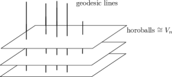
Figure 1: The horocycle decomposition at $\infty$. The horizontal planes are the horospheres based at $\infty$ (pictured in $\mathcal{H}^{3}$), and the vertical lines are the geodesics. Acting by $t\in A=A_{P_{\infty}}$ controls the flow along the geodesic, and acting by $v\in V_{n}$ changes position in the horosphere.

If $g\in\operatorname{SL}_{2}(B)$ has $g(\infty)=c\in\operatorname{Cusps}(B)$, the horocycle decomposition moves with it, and Figure 1 becomes Figure 2 where the planes (horospheres) move to the concentric circles tangent to the boundary at $c$, and the vertical geodesics move to semicircles with ends in the boundary which intersect the horospheres at $\infty$.

Figure 2: The horocycle decomposition at a point $x\in V_{n}$, which is the image of the horocycle decomposition at $\infty$, pictures in Figure 1. The horocycles/horospheres are the nested spheres, and the geodesics are semicircles between two points on the boundary. Note that they intersect the horospheres at infinity.

In [Borel1973], Borel and Serre define a compactification $H^{\operatorname{BS}}$ for symmetric spaces $H$ such that for torsion-free arithmetic groups $\Gamma$ the inclusion $\Gamma\setminus H\to\Gamma\setminus H^{\operatorname{BS}}$ is a homotopy equivalence. The Borel-Serre compactification of $\mathcal{H}^{n+1}$ comes from the horocycle decomposition associated to a boundary point $c\in\operatorname{Cusps}(B)$. The idea is to compactify the geodesic flow by letting $\lim_{t\to\infty}\pi_{v}(\pi_{t}(i_{n}))$ be an element of $\overline{A}\times N$. Here we use $s=1/t$ so that $s=0$ corresponds to $t=\infty$. The chart at infinity $H_{\infty}$ of the Borel-Serre compactification is given by

$$H_{\infty}=\overline{A_{\infty}}\times N_{\infty},$$ (40)

and, more generally, $H_{c}=\overline{A_{c}}\times N_{c}$. At $\infty$ we have $H_{\infty}\cong\mathbb{R}_{\geq 0}\times V_{n}.$ In this chart $\mathbb{R}_{>0}\times V_{n}\cong\mathcal{H}^{n+1}$ via $(s,v)\mapsto v+i_{n}(1/s)$, so we have compactified by adding all of the directions $v$ in which a geodesic can approach $\infty$. We do the same thing for every $c\in\operatorname{Cusps}(B)$ and Figure 2 becomes very striking.

Definition 5.6.3.

The partial Borel-Serre compactification of $\mathcal{H}^{n+1}$ relative to $\Gamma$ is defined to be $\mathcal{H}^{n+1,\operatorname{BS}}=\bigcup_{c\in\operatorname{Cusps}(B)}H_{c}$. In other words, it is $(\operatorname{Cusps}(B)\times\mathbb{R}_{\geq 0}\times V_{n})/\sim$ where $(c_{0},t_{0},v_{0})\sim(c_{1},t_{1},v_{1})$ if and only if $g_{t_{0},v_{0}}^{c_{0}}(i_{n})=g_{t_{1},v_{1}}^{c_{1}}(i_{n})$ when $t_{0}\neq 0$ and $t_{1}\neq 0$. Here $(c,t,v)\mapsto g^{c}_{t,v}$ takes the tuple to its corresponding element $g^{c}_{t,v}\in G(\mathbb{R})$ given by the Iwasawa decomposition at the cusp $c$.

The charts $\varphi_{c}:H_{c}\xrightarrow{\sim}\mathbb{R}_{\geq 0}\times\mathbb{R}^{n}$ make $\mathcal{H}^{n+1,\operatorname{BS}}$ a manifold with corners. In other words, every point has a neighborhood isomorphic to $\mathbb{R}^{n,j}=\mathbb{R}_{\geq 0}^{j}\times\mathbb{R}^{n-j}$ for some $0\leq j\leq n$, and $n$ is a continuous function of the point while $j$ is upper semicontinuous.

The prototypical manifold with corners is the closed positive “quadrant” $\mathbb{R}_{\geq 0}^{n}$ where the nonnegative parts of the coordinate hyperplanes are included. The basic properties of the category of manifolds with corners $\mathsf{Man}^{c}$ is developed in [Joyce2012] and [Joyce2014, §8.5-8.9]. In particular, there is a 2-category of orbifolds with corners $\mathsf{Orb}^{c}$ which can be developed from the perspective of charts, étale proper groupoids, and representable stacks in the category $\mathsf{Man}^{c}$ where the Grothendieck topology is given by open coverings. The theory is well-summarized in [Solomon2020, example 3.4] where the theory of quotient orbifolds is treated. The Borel-Serre compactification of $\mathcal{Y}(\Gamma)$ and $Y(\Gamma)$ are then defined to be objects of $\mathsf{Orb}^{c}$ and $\mathsf{Man}^{c}$, respectively, given by

$$\mathcal{X}^{\operatorname{BS}}(\Gamma)=[\Gamma\setminus\mathcal{H}^{n+1,\operatorname{BS}}],\quad X^{\operatorname{BS}}(\Gamma)=|\mathcal{X}^{\operatorname{BS}}(\Gamma)|.$$

We can now see that our orbifolds are more complicated to deal with because $\mathcal{X}(\Gamma):=[\Gamma\setminus\mathcal{H}^{n+1,\operatorname{Sat}}]$ and $X(\Gamma)=|\mathcal{X}(\Gamma)|$, and their status as spaces is unclear. We see that the charts $H_{c}$ of $\mathcal{H}^{n+1,\operatorname{BS}}$ are now blown down as shown in Figure 4. This can be pictured as a successive collapsing of cones as pictured in Figure 3, which readers may be more familiar with from Hatcher [Hatcher2002].

Figure 3: A pinching of the boundary of the cylinder $(-b,b)\times\mathbb{R}_{\geq 0}$ to a cone. In the above display, $I$ is the open interval $(-b,b)$.

Figure 4: A pinching of the boundary of $\mathbb{R}_{\geq 0}\times\mathbb{R}$ to a point.

We can see that the collapsed chart in two dimensions (Figure 4) can be parametrized by $(r,\theta)$ with $\theta\in(0,2\pi)$ and $r\geq 0$ where all of $(0,\theta)$ are identified. One can then see that these are equivalent to using charts which are locally homeomorphic to open subset of $\mathbb{R}_{>0}\times\mathbb{R}_{>0}\cup\{(0,0)\}$, which do not fall within the realm of manifolds with corners and are something else. To our knowledge, there is no theory of manifolds and orbifolds with “$o$-minimal corners” and the development of this theory is well beyond the scope of this paper.

We want to close this subsection with a comparison between the compactifications given and others existing in the literature. For the purposes of exposition, let us call the previously introduced the Satake compactifications the “easy Satake” compactifications. We will call the Satake compactification as used at the end of [Borel2019, Chapter 17] the “hard Satake” compactification. We will refer to the compactification used by Borel in [Borel2019, Chapter 17] and by EGM in [Elstrodt1988] as the “Borel compactification”.

In Borel’s construction from [Borel2019, Chapter 17], he selects a finite set of representatives for $\operatorname{Cusps}(G)=G(\mathbb{Q})/P(\mathbb{Q})$, which we will call $\{c_{1},\ldots,c_{h}\}$. Let $\Gamma^{c}=c^{-1}\Gamma c$, and $\Gamma^{c}_{\infty}$ is an extension of $\mathcal{O}_{c}^{\times}$ by $\Lambda_{c}$ where $\mathcal{O}_{c}^{\times}=\Gamma_{\infty}^{c}\cap M(\mathbb{Q})$ (contrary to what may be suggested by the notation, we do not know whether there is actually an order whose group of units is $\mathcal{O}_{c}^{\times}$).

Over every cusp $c\in\operatorname{Cusps}(G)$, one has a component

$$E_{c}=\Lambda_{c}\backslash M(\mathbb{R})U(\mathbb{R})/K\cap M(\mathbb{R})$$

on which

$$L_{c}=(\Gamma^{c}\cap P(\mathbb{Q}))/(\Gamma^{c}\cap U(\mathbb{Q}))\cong\Gamma_{\infty}^{c}/\Lambda_{c}\cong\mathcal{O}_{c}^{\times}$$

acts. Using the semidirect product structure, we see that

$$E_{c}\cong(\Lambda_{c}\backslash U(\mathbb{R}))\times(M(\mathbb{R})/M(\mathbb{R})\cap K)\cong(V_{n}/\Lambda_{c})\times 1.$$

Generally, there is some fibration $\sigma:E_{c}\to B_{c}$ with $B_{c}=M(\mathbb{R})/(M(\mathbb{R})\cap K)$ which is nontrivial, but in the rank one case this is always trivial, as can be verified directly ($M(\mathbb{R})$ is compact so $K\cap M(\mathbb{R})=M(\mathbb{R})$). When $U(\mathbb{R})$ is commutative (but $G$ is not necessarily rational rank 1), the hard Satake compactification is unique and would be the quotient of $E_{c}$ to obtain $B_{c}$. Since our case is rank one, and furthermore in our case $B_{c}$ is trivial, this implies that Satake’s hard compactification coincides with the easy compactification. So, in summary, the hard Satake compactification is equal to the easy Satake compactification, which is the blow-down of Borel-Serre, which is the blow-down of Borel. This language of “blow-down” is the language used by [Borel1973] and means that, in the map from Borel-Serre to Satake, the fibers over the cusps collapse to a point. It is also used to indicate that the cusp in the Satake compactification is replaced by many points, so that each geodesic terminating in the cusp in the Satake compactification now terminates in different points, each identified with the asymptotic direction in which the geodesics approached the cusp.

On the level of symmetric spaces, $\mathcal{H}^{n+1,\operatorname{BS}}=\mathcal{H}^{n+1,B}$, which is the addition of a copy of $S^{n}=V_{n}\cup\{\infty\}$ at each $c\in\operatorname{Cusps}(B)$.

First, we would like to say that our Satake compactification coincides with that of [Borel2019]. In general, there is a map from Borel to Borel-Serre by collapsing $B_{c}$ turning tori into spheres by collapsing the cycles, and there is a map from Borel-Serre to Satake by $\sigma$ which collapses the fibers completely to a point-cusp.

5.7 Satake Abelian Varieties

Satake gives a way to parametrize abelian varieties with certain specified endomorphism algebra [Satake1966, Proposition 3 and material before]. Using his theory, we can show that there is a construction depending on certain parameters where every $z\in\mathcal{H}^{n+1}$ corresponds to abelian varieties with “Clifford multiplication”. Satake’s construction generalizes both the Kuga-Satake construction, which associates to K3 surfaces abelian varieties of large dimension, and the theory of Shimura curves $[\Gamma\backslash\mathcal{H}^{2}]$, which parametrize abelian surfaces with quaternionic multiplication (see [Voight2020, Ch. 43] for an overview). Note in particular that the Shimura construction is closely related to integral ternary quadratic forms $Q$ via its even Clifford algebra $\operatorname{Clf}(Q)_{+}$; in the Satake generalization, we will use an indefinite form $Q$ for our abelian varieties.

Given a quadratic form $Q$ we consider the symmetric space $H=\operatorname{Spin}_{Q}(\mathbb{R})/K$ where $K$ is its maximal compact subgroup. Given an order $\mathcal{O}\subset B=\operatorname{Clf}(Q)_{\mathbb{Q}}$, we let $\Lambda=\mathcal{O}_{+}=\mathcal{O}\cap B_{+}$ and $V=(B_{+})_{\mathbb{R}}$. In the case that $Q$ has signature $(1,n+1)$ we have $H\cong\mathcal{H}^{n+1}$.

Theorem 5.7.1 ([Satake1966]).

The torus $V/\Lambda$ admits a family of complex structures $J_{z}:\mathcal{O}_{+}\to\mathcal{O}_{+}$ parametrized by $z\in H$, satisfying $J_{z}^{2}=-\operatorname{id}$ for every $z\in H$ and admitting a Riemann form.

In the case of signature $(1,n+1)$ a complex structure $J_{0}$ is determined by $b_{1}$ and $b_{2}$ described by the conditions in equations (41) and (42); it varies according to conjugation $g^{-1}J_{0}g$ for $g\in\operatorname{Spin}_{Q}(\mathbb{R})$. A Riemann form $E$ is given by a choice of $\mu\in\mathcal{O}^{+}$ described in equation (43).

In the case that the signature of $Q$ is $(1,n+1)$, the complex structure $J$, which depends on parameters $b_{1}$ and $b_{2}$, is given by

$$J(x)=xb_{1}+ixb_{2},\quad i=i_{1}i_{2}\ldots i_{n+1},\quad b_{1}\in\mathcal{O}_{+},\quad b_{2}\in\begin{cases}\mathcal{O}_{+},&n+1\mbox{ even }\\ \mathcal{O}_{-},&n+1\mbox{ odd }\end{cases}.$$ (41)

$$b_{1}^{2}+(-1)^{{n+1\choose 2}}b_{2}^{2}=-1,\quad b_{1}b_{2}+b_{2}b_{1}=0.$$ (42)

This makes $V=\mathbb{C}_{n+2}[j]_{+}$ into a complex vector space where $j$ is the generator of $C_{n+1,1}$ such that $j^{2}=1$. Give the lattice $\mathcal{O}_{+}$ a Riemann-form $E:\Lambda\times\Lambda\to\mathbb{Z}$ given by

$$E(x,y)=\operatorname{trd}(\mu x^{*}y),\qquad\mu\in\mathcal{O}_{+},\quad\mu^{*}=-\mu.$$ (43)

The general theory of Riemann forms is summarized succinctly in [Voight2020, 43.4.9,43.4.10]. Recall that this means $E:\Lambda\times\Lambda\to\mathbb{Z}$ is alternating, and $\mathbb{Z}$-bilinear with $\mathbb{R}$-linear extension $E_{\mathbb{R}}:V\to V$ such that $E_{\mathbb{R}}(Jx,Jy)=E_{\mathbb{R}}(x,y)$ for all $x,y\in\mathbb{C}_{n+1}[j]_{+}$ and the map $(x,y)\to E_{\mathbb{R}}(Jx,Jy)$ is a symmetric positive definite $\mathbb{R}$-bilinear form on $V$. These two conditions are equivalent to $H:V\times V\to\mathbb{R}[J]$ defined by $H(x,y)=E_{\mathbb{R}}(Jx,y)+JE_{\mathbb{R}}(x,y)$ being a positive definite Hermitian form on $V$ with $\operatorname{Im}(H)=E_{\mathbb{R}}$; so, given $H$ which is Hermitian positive definite on $V$ with $\operatorname{Im}H(\Lambda)\subset\mathbb{Z}$, then $\operatorname{Im}H|_{\Lambda}$ is a Riemann form for $(V,\Lambda)$.

By taking $[g]\in\operatorname{Spin}_{Q}(\mathbb{R})/K$ one can vary the complex structure by taking $J^{g}=g^{-1}Jg$. In our application we have $\operatorname{Spin}_{Q}(\mathbb{R})/K\cong\operatorname{SL}_{2}(\mathbb{C}_{n})/\operatorname{SU}_{2}(\mathbb{C}_{n})\cong\mathcal{H}^{n+1}$ with $[g]\mapsto g(i_{n})=z$ so $J_{z}=J^{g}$, and this map is well-defined. The $Q$ is the $Q$ coming from Bott periodicity, so $Q=x^{2}+yz+q$ where $q$ is our positive definite quadratic form of rank $n-1$. This means $Q$ has real signature $(1,n+1)$ and we have $\operatorname{Spin}_{Q}(\mathbb{R})/K\cong\operatorname{Spin}_{1,n+1}(\mathbb{R})/K\cong\operatorname{SL}_{2}(\mathbb{C}_{n})/\operatorname{SU}_{2}(\mathbb{C}_{n})\cong\mathcal{H}^{n+1}$. So to every $z\in\mathcal{H}^{n+1}$ we get a complex abelian variety $A_{z}$ such that $A(\mathbb{C})\cong(\operatorname{Clf}(Q)_{\mathbb{R}})_{+}/\Lambda$ where the complex structure and polarization are specified. Note that the dimension of $\operatorname{Clf}(Q)_{\mathbb{R}}$ is $m=\deg(Q)+1=(3+(n-1))+1=n+3$. This implies the abelian variety $A_{z}$ has complex dimension $2^{m-2}=2^{n+1}$; hence via this Satake construction of abelian varieties (depending on choices $\mu$, $b_{1},b_{2}$) the symmetric space $\mathcal{H}^{n+1}$ actually parametrizes polarized abelian varieties of dimension $2^{n+1}$ with $\mathcal{O}_{+}\subset\operatorname{End}(A_{z})$ for every $z\in\mathcal{H}^{n+1}$.

Note that quotients of $\mathcal{H}^{2}$ parametrize complex abelian surfaces with a fixed quaternionic multiplication, while quotients of $\mathcal{H}^{3}$ parametrize complex abelian fourfolds $A$ with $\operatorname{End}(A/\mathbb{C})=\mathcal{O}_{+}$ with $\dim_{\mathbb{Q}}(\mathcal{O}_{+}\otimes_{\mathbb{Z}}\mathbb{Q})=8$ for some fixed order $\mathcal{O}$.

6 Arithmeticity of $\operatorname{SL}_{2}(\mathcal{O})$

The aim of this section is to prove that $\operatorname{SL}_{2}(\mathcal{O})$ can be viewed as an arithmetic subgroup of $\operatorname{SO}_{1,n+1}(\mathbb{R})$. This is done in Theorem 6.1.4. This has consequences for our fundamental domains because the Borel–Harish-Chandra Theorem then implies that the group action is discrete and finite covolume. This has abstract consequences for the construction of our fundamental domain constructions in section 7 (although we don’t make use of the general constructions of Fundamental domains of Borel in [Borel2019], which are difficult to work with in practice and do not mirror the classical constructions in $\mathcal{H}^{2}$ and $\mathcal{H}^{3}$).

Discussions of arithmeticity of the groups $\operatorname{PSL}_{2}(\mathcal{O})$ for $\mathcal{O}=\mathbb{Z}[i_{1},\ldots,i_{n-1}]$ exist in the literature but notation and terminology varies. Because of this, in section 6.1 we give a definition of arithmetic subgroups of semisimple real Lie groups in terms of group schemes over the integers. We are also careful to emphasize that this notion is a property of a subgroup $\Gamma$ of a real Lie group and not an abstract property of a group $\Gamma$.

6.1 Arithmetic Groups

We take [Morris2015, Definition 5.1.19] as a basis for our definition of arithmetic group—the only change (other than style) is that we are careful not to take $\mathbb{Z}$-points of $\mathbb{Q}$-group schemes (see Appendix B for a discussion of $\mathbb{Z}$-points of $\mathbb{Q}$-group schemes and why this is deprecated).

Definition 6.1.1.

Let $H$ be a semisimple Lie group and $\Gamma$ be a subgroup. We say that $\Gamma<H$ is an arithmetic subgroup or $(\Gamma,H)$ is an arithmetic pair if and only if one of the following holds:

1. (Base Case: Integer Points of Group Schemes) There exists an integer $n$ and a closed $\mathbb{Z}$-subgroup scheme $G\subset\operatorname{SL}_{n}$ such that there exists an isomorphism of Lie groups $\phi:H\stackrel{{\scriptstyle\cong}}{{\to}}G(\mathbb{R})$ such that $\phi(\Gamma)=G(\mathbb{Z})$.

2. (Taking Commensurable Groups) The group $\Gamma<H$ is commensurable to $\Gamma^{\prime}<H$ for $(\Gamma^{\prime},H)$, an arithmetic pair.

3. (Taking Connected Components) The pair $(\Gamma,H)$ comes from taking connected components of a known arithmetic pair $(\Gamma^{\prime},H^{\prime})$, i.e., $(\Gamma,H)\cong(\Gamma^{\prime}\cap(H^{\prime})^{0},(H^{\prime})^{0}).$

4. (Taking Quotients by Compacts) The pair $(\Gamma,H)$ comes from taking the quotient of a known arithmetic pair $(\Gamma^{\prime},H^{\prime})$ by a compact normal subgroup of $K^{\prime}<H^{\prime}$, i.e. $(\Gamma,H)\cong(\Gamma^{\prime}/(\Gamma^{\prime}\cap K^{\prime}),H^{\prime}/K^{\prime}).$

Remark 6.1.2.

Note that $K^{\prime}$ can be taken to be a finite group above. Thus the quotient of an arithmetic group by a finite subgroup is arithmetic.

Remark 6.1.3.

When $(\Gamma,H)$ is an arithmetic pair we sometimes call $\Gamma$ simply an arithmetic group. While this terminology, which omits the ambient group, is often used in the literature, we emphasize that being a subgroup of a particular group is an important part of the definition. We point out some variations. In [Krausshar2004], Kraußhar takes “arithmetic group” to mean discrete subgroup (without any reference to an algebraic group). The authors of [Maclachlan1989] and [Maclachlan2003] define an “arithmetic group” to be commensurable with the $\mathbb{Z}$-points of some group scheme over $\mathbb{Z}$ (the emphasis here is on the $\exists$ quantifier on the group). In [Morris2015] (and most other references on arithmetic groups), an arithmetic group is taken to be the $\mathbb{Z}$-points of a group scheme defined over $\mathbb{Q}$.

Theorem 6.1.4 (Arithmeticity).

Let $\varphi:\operatorname{PSL}_{2}(\mathbb{C}_{n})\to\operatorname{O}_{1,n+1}(\mathbb{R})^{\circ}$ be the isomorphism of groups given first by acting via Möbius transformations on $\mathcal{H}^{n+1}$ and then by identifying orientation-preserving isometries of $\mathcal{H}^{n+1}$ with $\operatorname{O}_{1,n+1}(\mathbb{R})^{\circ}$. Let $\Gamma=\operatorname{PSL}_{2}(\mathcal{O})\subset\operatorname{PSL}_{2}(\mathbb{C}_{n})$ for $\mathcal{O}=\left(\frac{-d_{1},\ldots,-d_{n-1}}{\mathbb{Z}}\right)$ with $q=d_{1}x_{1}^{2}+\cdots+\cdots+d_{n-1}x_{n-1}^{2}$, a positive definite quadratic form over $\mathbb{Z}$. The group $\varphi(\Gamma)$ is an arithmetic subgroup of $\operatorname{O}_{Q}(\mathbb{R})$ where $Q=x^{2}-yz+q$.

Proof.

In this proof we work with two distinct representations of $\Gamma$ into $\operatorname{O}_{Q}(\mathbb{R})^{\circ}$: the first is the representation $\varphi$ coming from Möbius transformations as in the statement, and the second, which we will call $\psi$, comes from the isomorphism of $\mathbb{Z}$-schemes $\operatorname{SL}_{2}(\operatorname{Clf}_{q})\to\operatorname{Spin}_{Q}\to\operatorname{O}_{Q}$ of Theorem 4.2.3, which we will call “the Spin isomorphism”.

This proof is a fortiori. For any two abstract isomorphisms $\varphi,\psi:G_{0}\to G_{1}$ of abstract groups $G_{1}$ and $G_{0}$, there exists an automorphism $\sigma$ of $G_{1}$ such that $\sigma=\psi\varphi^{-1}$. Assuming $\psi(\Gamma)$ is an arithmetic subgroup, then by part (1) of Definition 6.1.1 the group $\sigma(\psi(\Gamma))=\varphi(\Gamma)$ is also an arithmetic subgroup.

We now prove that $\psi(\Gamma)$ is an arithmetic subgroup of $\operatorname{SO}_{1,n+1}(\mathbb{R})=\operatorname{SO}_{Q}(\mathbb{R})$. Since the morphism of $\mathbb{Z}$-group schemes $\operatorname{SL}_{2}(\operatorname{Clf}_{q})\to\operatorname{O}_{Q}$ is defined via a conjugation action, it descends to an injective morphism of $\mathbb{Z}$-group schemes $\operatorname{PSL}_{2}(\operatorname{Clf}_{q})\to\operatorname{O}_{Q}$. We will show that $\Gamma=\operatorname{PSL}_{2}(\mathcal{O})$ has finite index in $\operatorname{SO}_{Q}(\mathbb{Z})$, which is of finite index. This will prove the result.

First, observe that we have $\operatorname{Spin}_{Q}(\mathbb{Z})\cong\operatorname{SL}_{2}(\mathcal{O})$ since $\operatorname{SL}_{2}(\operatorname{Clf}_{q})\cong\operatorname{Spin}_{Q}$ as $\mathbb{Z}$-group schemes (Theorem 4.2.3). Using the short exact sequence of fppf sheaves of groups over $\operatorname{Spec}(\mathbb{Z})$ (Theorem 4.2.4), we get the associated long exact sequence

$$1\to\mu_{2}(\mathbb{Z})\to\operatorname{Spin}_{Q}(\mathbb{Z})\to\operatorname{SO}_{Q}(\mathbb{Z})\to H^{1}(\operatorname{Spec}(\mathbb{Z})_{\operatorname{fppf}},\mu_{2}).$$

We will now compute $|H^{1}(\operatorname{Spec}(\mathbb{Z})_{\operatorname{fppf}},\mu_{2})|=2$, which will prove that the image of $\operatorname{Spin}_{Q}(\mathbb{Z})$ (which is the image of $\Gamma$) inside $\operatorname{SO}_{Q}(\mathbb{Z})$ has finite index, and give the result.

To see this, we use the Kummer sequence for multiplication by 2 in the fppf topology on $\operatorname{Spec}(\mathbb{Z})$,

$$1\to\mu_{2}\to\mathbb{G}_{m}\xrightarrow{[2]}\mathbb{G}_{m}\to 1.$$

The long exact cohomology sequence of a short exact sequence ([Knus1991, III 2.6.1]) gives

$$1\to\mu_{2}(\mathbb{Z})\to\mathbb{G}_{m}(\mathbb{Z})\xrightarrow{[2]}\mathbb{G}_{m}(\mathbb{Z})\to H^{1}(\operatorname{Spec}(\mathbb{Z})_{\operatorname{fppf}},\mu_{2})\to H^{1}(\operatorname{Spec}(\mathbb{Z})_{\operatorname{fppf}},\mathbb{G}_{m}).$$

We have $\mu_{2}(\mathbb{Z})=\mathbb{G}_{m}(\mathbb{Z})=\mathbb{G}_{m}(\mathbb{Z})=\{\pm 1\}$, and the image of the map $[2]:\mathbb{G}_{m}(\mathbb{Z})\to\mathbb{G}_{m}(\mathbb{Z})$ is the map sending $-1$ to $1$. Also, by [Knus1991, III 2.7.4] we can compare the fppf topology to the étale topology to conclude that $H^{1}(\operatorname{Spec}(\mathbb{Z})_{\operatorname{fppf}},\mathbb{G}_{m})=\operatorname{Pic}(\mathbb{Z})=1$. This proves that $\{\pm 1\}=\mathbb{G}_{m}(\mathbb{Z})\to H^{1}(\operatorname{Spec}(\mathbb{Z})_{\operatorname{fppf}},\mu_{2})$ is surjective with trivial kernel and hence an isomorphism. ∎

Remark 6.1.5.

It is necessary to move to the fppf topology here as the sequences are not exact in the étale topology. See for example [Knus1991, III.2.7.3 part (3)]. Write $\mathbb{Z}_{(p)}^{\operatorname{sh}}$ for the strict Henselization of the localization of $\mathbb{Z}$ at the prime $p$. Above primes $p\neq 2$ and the generic point, the morphism $\mathbb{G}_{m}(\mathbb{Z}_{(p)}^{\operatorname{sh}})\xrightarrow{[2]}\mathbb{G}_{m}(\mathbb{Z}_{(p)}^{\operatorname{sh}})$ is surjective, so exactness of the Kummer and Spin sequences can be checked on $\operatorname{Spec}(\mathbb{Z})_{\operatorname{\acute{e}t}}$ by [Auel2009, Proposition 1.41]. We cannot use this result for $p=2$ because the morphism $\mathbb{G}_{m}(\mathbb{Z}_{(2)}^{\operatorname{sh}})\to\mathbb{G}_{m}(\mathbb{Z}_{(2)}^{\operatorname{sh}})$ given by $t\mapsto t^{2}$ is not surjective, and hence the $2$-Kummer sequence is not exact in the étale topology. Knowing this, one might naively try to show that the morphism is exact on the fppf stalks as can be done for proofs using the étale topology away from $2$. This is extremely difficult, however, as the stalks in the fppf topology are not easy to describe: see [mathoverflow-grothendieck-topology, MO42258].

6.2 Borel–Harish-Chandra

Definition 6.2.1.

Let $H$ be a Lie group. A lattice $\Gamma<H$ is a subgroup which is discrete and has finite covolume with respect to the Haar measure on $H$.

Theorem 6.2.2 (Borel–Harish-Chandra).

Let $H$ be a semisimple Lie group. If $\Gamma<H$ is an arithmetic group, then $\Gamma$ is a lattice.

Proof.

See [Morris2015, Major Theorem 5.1.11]. See also [Platonov1994, Theorem 4.8]. ∎

Corollary 6.2.3.

If $\Gamma<H$ is an arithmetic group, then it acts properly discontinuously by left multiplication on $H$. It will also act properly discontinuously on $H/K$ for $K$ a maximal compact subgroup.

Proof.

See [Boothby1986, p. 96]. See also [math-stack-exchange-left-translation, MSE186183]. ∎

7 Fundamental Domains for $\operatorname{PSL}_{2}(\mathcal{O})$

Let $\mathcal{O}=\left(\frac{-d_{1},\ldots,-d_{n-1}}{\mathbb{Z}}\right)\subset\mathbb{C}_{n}$ for $d_{j}\in\mathbb{Z}$ squarefree coprime integers. Let $\Gamma=\operatorname{PSL}_{2}(\mathcal{O})$. In this section we give a construction of the open fundamental domain $D\subset\mathcal{H}^{n+1}$ for $\Gamma$. Interestingly, the proof is a “proof by moduli interpretation”. Here, we first show that every point in $\mathcal{H}^{n+1}$ is in $\operatorname{SL}_{2}(\mathbb{C}_{n})$-bijection with a homothety class of positive definite Clifford-Hermitian matrices. We then classify the elements $x$ of a $\Gamma$-orbit in $\mathcal{H}^{n+1}$ with maximal $x_{n}$ as those which correspond to homothety classes of Hermitian forms achieving a minimal value at a certain standard point.

This mirrors the theory of quadratic forms in $\operatorname{SL}_{n}(\mathbb{R})$ and the theory of Hermitian forms in $\operatorname{SL}_{2}(\mathbb{C})$ but with some stranger definitions. This section further develops Bianchi-Humbert Theory and is inspired by section 3 of [Swan1971].

7.1 Special $\mathcal{O}$ and Stabilizers of $\infty$

At times we will need to talk about stabilizers of $\infty$ and the Clifford group of $\mathcal{O}$. In this section we suppose that $\mathcal{O}$ is $*$-stable, i.e., that $\mathcal{O}^{*}=\mathcal{O}$; the stronger assumption that $\mathcal{O}$ is Clifford-stable (Definition 3.1.3) is unnecessary.

Definition 7.1.1.

Recall that $\mathcal{O}^{\times}$, the group of Clifford units of $\mathcal{O}$, is defined to be $U(\mathcal{O})\cap\mathbb{C}_{n}^{\times}$. We say that $\mathcal{O}$ is special if $\mathcal{O}^{\times}\neq\{\pm 1\}$. In this case we will also say that $\Gamma=\operatorname{PSL}_{2}(\mathcal{O})$ and $\Gamma\backslash\mathcal{H}^{n+1}$ are special.

Lemma 7.1.2.

The stabilizer group $\operatorname{SL}_{2}(\mathcal{O})_{\infty}$ is generated by matrices of the form $\tau_{s}=\left(\begin{smallmatrix}1&s\\ 0&1\end{smallmatrix}\right)$, and $\sigma_{t}=\left(\begin{smallmatrix}t&0\\ 0&t^{*-1}\end{smallmatrix}\right),$ for $s\in\operatorname{Vec}(\mathcal{O})$, and $t\in\mathcal{O}^{\times}.$ In fact $\operatorname{SL}_{2}(\mathcal{O})_{\infty}\cong\operatorname{Vec}(\mathcal{O})\rtimes\mathcal{O}^{\times}$. In fact $\operatorname{SL}_{2}(\underline{\mathcal{O}})_{\infty}\cong\operatorname{Vec}(\underline{\mathcal{O}})\rtimes\underline{\mathcal{O}}^{\times}$ as group schemes.

Proof.

We know that they must be upper triangular of the form $g=\left(\begin{smallmatrix}a&b\\ 0&d\end{smallmatrix}\right)\in\Gamma$. The condition $\Delta(g)=ad^{*}=1$ implies that $d^{*}=a^{-1}$ or $d=a^{*-1}$. We can factor these matrices as $\left(\begin{smallmatrix}a&b\\ 0&a^{*-1}\end{smallmatrix}\right)=\left(\begin{smallmatrix}a&0\\ 0&(a^{*})^{-1}\end{smallmatrix}\right)\left(\begin{smallmatrix}1&a^{-1}b\\ 0&1\end{smallmatrix}\right),$ so the matrices of the form $\tau_{s}=\left(\begin{smallmatrix}1&s\\ 0&1\end{smallmatrix}\right)$ and $\sigma_{t}=\left(\begin{smallmatrix}t&0\\ 0&t^{*-1}\end{smallmatrix}\right)$ generate $\Gamma_{\infty}$. ∎

Corollary 7.1.3.

The group $\Gamma=\operatorname{PSL}_{2}(\mathcal{O})$ is special if and only if $\Gamma_{\infty}$ is larger than $\Lambda=\operatorname{Vec}(\mathcal{O})$.

7.2 Clifford-Hermitian Matrices

The Clifford adjoint of an $m\times n$ matrix $A\in M_{m,n}(\mathbb{C}_{n})$ is the $n\times m$ matrix $A^{{\dagger}}\in M_{n,m}(\mathbb{C}_{n})$ given by taking the conjugate transpose:

$$A^{{\dagger}}=(\overline{A})^{\operatorname{t}}=\overline{(A^{\operatorname{t}})}.$$

Definition 7.2.1.

We say $A\in M_{2}(\mathbb{C}_{n})$ is Clifford-Hermitian (or simply Hermitian for convenience) if and only if it has Clifford vector entries and $A=A^{{\dagger}}$. We denote the collection of $2\times 2$ Clifford-Hermitian matrices by $M_{2}(\mathbb{C}_{n})_{\operatorname{herm}}$.

Note that if $A$ is Hermitian, then it has the form

$$A=\begin{pmatrix}a&b\\ \overline{b}&c\end{pmatrix},\qquad a,c\in\mathbb{R},\quad b\in V_{n}.$$

We now define the discriminant, positive definiteness, and homothety (cf. [Elstrodt1988, Section 3]).

Definition 7.2.2.

Let $A=\left(\begin{smallmatrix}a&b\\ \overline{b}&c\end{smallmatrix}\right)$ be Hermitian.

1. Its discriminant (or naive determinant) is defined to be the real number $\det(A)=ac-|b|^{2}.$

2. We say $A$ is positive definite if and only if $a,c>0$ and $\det(A)>0$. We will denote the cone of positive definite Hermitian matrices by $M_{2}(\mathbb{C}_{n})_{\operatorname{herm}}^{\operatorname{pos}}$.

3. Two positive definite matrices $A$ and $B$ are homothetic if and only if there exists some $k\in\mathbb{R}_{>0}$ such that $A=kB$.

Note that in the definition of positive definite it suffices to take either $a>0$ or $c>0$. Also note that the notation is such that if $A=\left(\begin{smallmatrix}a&b\\ \overline{b}&c\end{smallmatrix}\right)\in M_{2}(\mathbb{C}_{n})_{\operatorname{herm}}^{\operatorname{pos}}$ then $b\in V_{n}$. So, the index of the Clifford vectors and the index on the collection of positive definite matrices do not coincide. The $n+1$ in the subscript of $M_{2}(\mathbb{C}_{n})_{\operatorname{herm}}^{\operatorname{pos}}$ denotes the real dimension of the space of matrices. In the future we will let $\overline{M_{2}(\mathbb{C}_{n})}_{\operatorname{herm}}^{\operatorname{pos}}=M_{2}(\mathbb{C}_{n})_{\operatorname{herm}}^{\operatorname{pos}}/\mathbb{R}_{>0}^{\times}$ be the collection of positive definite Hermitian matrices up to homothety.

Theorem 7.2.3.

There is a well-defined left action of $\operatorname{SL}_{2}(\mathbb{C}_{n})$ on $M_{2}(\mathbb{C}_{n})_{\operatorname{herm}}^{\operatorname{pos}}$ given by $g\cdot A=gAg^{{\dagger}}$. This action respects homothety in the sense that $A$ and $B$ are homothetic if and only if $g\cdot A$ and $g\cdot B$ are for each $g\in\operatorname{SL}_{2}(\mathbb{C}_{n})$.

Proof.

This is [Elstrodt1988, Prop 3.3]. ∎

7.3 Clifford-Hermitian Matrices and the Action of $\operatorname{SL}_{2}$

In section 3 of [Elstrodt1988], Elstrodt, Grunewald, and Mennicke give a $\operatorname{SL}_{2}(\mathbb{C}_{n})$-equivariant bijection between homothety classes of positive definite matrices and $\mathcal{H}^{n+1}$. We will make use of this bijection and develop a further relationship which will help us give a formula for the boundary of the fundamental domain of $\Gamma$.

Theorem 7.3.1.

The map $\Phi:\overline{M_{2}(\mathbb{C}_{n})}_{\operatorname{herm}}^{\operatorname{pos}}\to\mathcal{H}^{n+1}$ given by

$$\begin{pmatrix}a&b\\ \overline{b}&c\end{pmatrix}\mapsto\dfrac{b}{c}+i_{n}\dfrac{\sqrt{ac-|b|^{2}}}{c}$$

is an $\operatorname{SL}_{2}(\mathbb{C}_{n})$-equivariant bijection. The inverse is given by

$$\Phi(z+i_{n}\zeta)=\begin{pmatrix}\zeta+|z|^{2}&cz\\ c\overline{z}&c\end{pmatrix}$$

for some choice of $c>0$. Here we are writing $x\in\mathcal{H}^{n+1}$ as $x=z+i_{n}\zeta$ where $\zeta\in\mathbb{R}_{>0}$ and $z\in V_{n}$.

Proof.

This is [Elstrodt1988, Prop. 3.4] and [Elstrodt1988, Prop 3.5]. They show that there exists an inverse map $\Psi:\mathcal{H}^{n+1}\to M_{2}(\mathbb{C}_{n})_{\operatorname{herm}}^{\operatorname{pos}}$ which is the “Hermitian form associated to $x$” that we will see in Theorem 7.7.5, (2). The second part is implicit in the proof of Theorem 7.3.3 which we will delay. ∎

We will need some enhancements to this map.

Definition 7.3.2.

Let $A\in\overline{M_{2}(\mathbb{C}_{n})}_{\operatorname{pos}}^{\operatorname{herm}}$. The Hermitian form associated to $A$ is the map $q_{A}:\mathbb{C}_{n}^{2}\to\mathbb{R}$ given by

$$q_{A}(w)=w^{{\dagger}}Aw,\qquad w=\begin{pmatrix}u\\ v\end{pmatrix}.$$ (44)

Under certain circumstances we can complete the square. This gives a description of the map $\Phi$ from [Elstrodt1988] in terms of these parameters.

Theorem 7.3.3.

Let $A=\left(\begin{smallmatrix}a&b\\ \bar{b}&c\end{smallmatrix}\right)$ be a positive definite Hermitian matrix. Let $w=\begin{pmatrix}u\\ v\end{pmatrix}$ and suppose that $u,v\in\mathbb{C}_{n}^{\vartriangleright}\cup\{0\}$ are such that there exists a matrix

$$\begin{pmatrix}u&*\\ v&*\end{pmatrix}\in\operatorname{GL}_{2}(\mathbb{C}_{n}).$$ (45)

1. We may write the Hermitian form as

   $$q_{A}(w)=a|u|^{2}+2\operatorname{Re}(\overline{u}bv)+c|v|^{2}.$$ (46)

2. With $w$ as above, if we let $z=b/c\in V_{n}$ ($c$ is real) and $\zeta=\sqrt{ac-|b|^{2}}/c$, then

   $$q_{A}(w)=c\left(|\zeta u|^{2}+|\bar{z}u+v|^{2}\right),\qquad w=\begin{pmatrix}u\\ v\end{pmatrix}.$$

Proof.

1. Here we just have

   $$w^{{\dagger}}Aw =\bar{u}(au+bv)+\bar{v}(\bar{b}u+cv)$$

   $$=a|u|^{2}+\bar{u}bv+\bar{v}\bar{b}u+c|v|^{2}$$

   $$=a|u|^{2}+2\operatorname{Re}(\bar{u}bv)+c|v|^{2}.$$

   We only used the fact that for $\alpha\in\mathbb{C}_{n}^{\vartriangleright}$, that $|\alpha|^{2}=\alpha\overline{\alpha}=\overline{\alpha}\alpha$ and that $\alpha+\overline{\alpha}=2\operatorname{Re}(\alpha)$.

2. We will show that $\bar{z}u+v\in\mathbb{C}_{n+1}^{\vartriangleright}$, so that we may expand $|\bar{z}u+v|^{2}$ in terms of conjugates. We have $\bar{z}u+v=(\bar{z}+vu^{-1})u$. The condition (45) implies that $uv^{-1}\in V_{n}$ and hence that $vu^{-1}\in V_{n}$ since multiplicative inverses of Clifford vectors are Clifford vectors. This proves that $\bar{z}+vu^{-1}\in V_{n}$. Since the product of a Clifford vector and a Clifford group element is a Clifford group element, we have shown that $|\bar{z}u+v|=\overline{(\bar{z}u+v)}(\bar{z}u+v)=(\bar{z}u+v)\overline{(\bar{z}u+v)}$.

   We get

   $$\zeta^{2}|u|^{2}+|\bar{z}u+v|^{2}= \zeta^{2}|u|^{2}+|z|^{2}|u|^{2}+\overline{\bar{z}u}v+\overline{v}\bar{z}u+|v|^{2}$$

   $$=(\zeta^{2}+|z|^{2})|u|^{2}+2\operatorname{Re}(\bar{u}zv)+|v|^{2}.$$

   Now, multiplying the above expression by $c$ and matching terms with (46) we find $a/c=(\zeta^{2}+|z|^{2})$ and $b/c=z$ give a solution. This gives $z=b/c$ and $\zeta^{2}=(ac-|b|^{2})/c^{2}$ or $\zeta=\sqrt{ac-|b|^{2}}/c$.

∎

From now on we will allow ourselves to conflate $\overline{M_{2}(\mathbb{C}_{n})}_{\operatorname{herm}}^{\operatorname{pos}}$ and $\mathcal{H}^{n+1}$ using this $\operatorname{PSL}_{2}(\mathbb{C}_{n})$-equivariant bijection.

7.4 Unimodular Pairs

We remind the reader that we call $ab^{-1}$ left division and $b^{-1}a$ right division, following conventions in the literature (cf. Remark 3.4.2).

We need an equivariance statement here that describes the relation between the matrix of the same transformation in two different sets of coordinates. This is analogous to the classical statement that an inner product space whose inner product is given by the matrix $M$ in a fixed basis has the matrix $A^{T}MA$ when the basis is changed by the action of $A$.

We record this in the form of a lemma for future reference.

Lemma 7.4.1.

For all $g\in\operatorname{SL}_{2}(\mathbb{C}_{n})$, all $A\in P$, and all $w\in\mathbb{C}_{n}^{2}$, we have $q_{A}(gw)=q_{g^{{\dagger}}Ag}(w)$.

Proof.

For $w^{{\dagger}}$, a unimodular row vector, we have $q_{A}(w)=w^{\dagger}Aw$. Then acting on the left of $w$ gives $q_{A}(gw)=(gw)^{{\dagger}}A(gw)=w^{{\dagger}}g^{{\dagger}}Agw=q_{g^{{\dagger}}Ag}(w)$. ∎

To make sense of this, we translate the coprimeness condition to a condition about matrices. Equivalently, they could appear as any other row or any column. We are going to use this observation to generalize this to the noncommutative setting.

7.5 Cusps and Ideal Classes

Consider $\operatorname{Clf}(q)$ for $q$ a positive definite quadratic form in $n-1$ variables. Let $K=\operatorname{Clf}(q)\otimes\mathbb{Q}$. Let $\mathcal{O}$ be an order in $K$. Let $\widehat{V}=\operatorname{Vec}(K)\cup\{\infty\}$. Let $\Gamma=\operatorname{PSL}_{2}(\mathcal{O})$. The aim of this section is to prove that $\Gamma\backslash\widehat{V}$ is finite using ideal classes.

The terminology of ideals is borrowed from [Reiner1975]. We build on some terminology from §3. By a left $\mathcal{O}$-lattice $L$ we mean a finitely generated left $\mathcal{O}$-module. When $L$ is a subset of a free left $K$-module $M$, we call it full if $\mathbb{Q}L=M$. By a fractional ideal in $K$ we mean a full left $\mathcal{O}$-lattice in $M=K$. Since an isomorphism of fractional ideals induces an automorphism of $K$, we have that $I\cong J$ if and only if there exists some $a\in K^{\times}$ such that $I=Ja$.

Definition 7.5.1.

Given two fractional ideals $I,J\subset K$, we declare them to be equivalent if and only if there exists some unit $a\in K^{\times}$ such that $I=Ja$. We will write $I\sim J$ when this is the case. The set of equivalence classes will be denoted by $\operatorname{Cl}(\mathcal{O})$ and called the left ideal class set.

We use the finiteness of the set of ideal classes.

Theorem 7.5.2 (Jordan-Zassenhaus [Reiner1975, Theorem 26.4]).

If $\mathcal{O}$ is an order in a semisimple $\mathbb{Q}$-algebra $K$, then there are only finitely many isomorphism classes of left $\mathcal{O}$-lattices of any given $\mathbb{Z}$-rank. As a consequence, $\operatorname{Cl}(\mathcal{O})$ is a finite set.

This applies to our situation, as $q$ is nondegenerate so $\operatorname{Clf}(q)_{\mathbb{Q}}=L$ is semisimple. (If the arity $n-1$ of the quadratic form is even it is central simple.)

We record the following Lemma relating the notion of equivalence to generation of ideals.

Lemma 7.5.3.

Suppose that $(c,d)\in\mathcal{O}^{2}$ is unimodular. Then

1. $\mathcal{O}c^{*}+\mathcal{O}d^{*}=\mathcal{O}$ as left $\mathcal{O}$-ideals;

2. $c\mathcal{O}^{*}+d\mathcal{O}^{*}=\mathcal{O}^{*}$ as right $\mathcal{O}^{*}$-ideals;

3. $\mathcal{O}\overline{c}+\mathcal{O}\overline{d}=\mathcal{O}$ as left $\mathcal{O}$-ideals;

4. $c\mathcal{O}+d\mathcal{O}=\mathcal{O}$ as right $\mathcal{O}$-ideals.

Proof.

Suppose that $\gamma=\left(\begin{smallmatrix}a&b\\ c&d\end{smallmatrix}\right)\in\operatorname{SL}_{2}(\mathcal{O})$. Then $ad^{*}-bc^{*}=1$, which implies that $-b(c^{*})+ad^{*}=1$, which implies that $\mathcal{O}=\mathcal{O}c^{*}+\mathcal{O}d^{*}$. This can also seen by multiplying $\gamma^{-1}$ on the left by $\gamma$. The second part follows from applying the $*$ operation. The third part follows from the existence of a left matrix inverse for $\left(\begin{smallmatrix}\bar{c}&*\\ \bar{d}&*\end{smallmatrix}\right)$. The fourth part follows from the existence of a right matrix inverse for a matrix of the form $\left(\begin{smallmatrix}c&d\\ *&*\end{smallmatrix}\right)$. ∎

Theorem 7.5.4.

As before, suppose that $\mathcal{O}$ is an order closed under the Clifford conjugations inside $\left(\frac{-d_{1},\ldots,-d_{n}}{\mathbb{Q}}\right)$. Then there is a well-defined injective map from $\Gamma\backslash\widehat{V}\to\operatorname{Cl}(\mathcal{O})$.

Proof.

We can define a map from $f:\widehat{K}\to\operatorname{FIdeals}_{\mathcal{O}}(K)$ to ideals via $f(x)=\mathcal{O}x+\mathcal{O}$ if $x\neq\infty$ and $f(\infty)=\mathcal{O}$. We claim that this is well-defined on equivalence classes. Let $g=\left(\begin{smallmatrix}a&b\\ c&d\end{smallmatrix}\right)$ be an element of $\Gamma$, and let $y\in K$; take $x=gy=(ay+b)(cy+d)^{-1}$. We then have $\mathcal{O}x+\mathcal{O}=\mathcal{O}(ay+b)(cy+d)^{-1}+\mathcal{O}\cong\mathcal{O}(ay+b)+\mathcal{O}(cy+d)$. This module contains the elements $d^{*}(ay+b)-b^{*}(cy+d)=y$ and $a^{*}(cy+d)-c^{*}(ay+b)=1$, by Corollary 2.8.8, so it contains $\mathcal{O}y+\mathcal{O}$; the reverse inclusion is clear, so we see that $\mathcal{O}x+\mathcal{O}\cong\mathcal{O}y+\mathcal{O}$. Also note that if $g(\infty)=ac^{-1}=x$, then $\mathcal{O}x+\mathcal{O}\cong\mathcal{O}a+\mathcal{O}c=\mathcal{O}$. ∎

Corollary 7.5.5.

For any order $\mathcal{O}$, even if not closed under the Clifford conjugations, the set $\Gamma\backslash\widehat{V}$ is finite.

Proof.

If $\mathcal{O}$ is closed under the Clifford conjugations, this follows from Theorem 7.5.4, because we have given an injection from this set to the finite set $\operatorname{Cl}(\mathcal{O})$. In general, let $\mathcal{O}_{c}=\mathcal{O}\cap\mathcal{O}^{*}\cap\bar{\mathcal{O}}\cap\mathcal{O}^{\prime}$. Then $\mathcal{O}_{c}$ is certainly closed under the Clifford conjugations, and so there are only finitely many equivalence classes of cusps for $\mathcal{O}_{c}$. Since $\mathcal{O}_{c}$-equivalent cusps are $\mathcal{O}$-equivalent, the more general statement follows. ∎

Remark 7.5.6.

One also prove finiteness of the quotient of cusps using abstract properties of arithmetic groups following [Borel2019, Proposition 15.6]. This is what [Elstrodt1988, Prop 6.2] does. Our proof gives connections to ideal class sets and holes in lattices and, more importantly, is algorithmic.

7.6 Characterization of Spheres

Theorem 7.6.1.

Let $u,v\in\mathbb{C}_{n}^{\vartriangleright}$ be such that there exists a matrix $\left(\begin{smallmatrix}u&*\\ v&*\end{smallmatrix}\right)\in\operatorname{GL}_{2}(\mathbb{C}_{n})$. Let $x\in\mathcal{H}^{n+1}$ and let $[A]\in\overline{M_{2}(\mathbb{C}_{n})}_{\operatorname{herm}}^{\operatorname{pos}}$ be its corresponding homothety class of positive definite matrices.

The condition $q_{A}(u,v)\geq q_{A}(0,1)$ on the matrix $A$ is equivalent to the condition that $x$ lies outside $B(-\bar{u}^{-1}\bar{v})$ where $-\bar{u}^{-1}\bar{v}\in\operatorname{Vec}(K)=\partial\mathcal{H}^{n+1}$. The radius of $B(-\bar{u}^{-1}\bar{v})$ is $1/|\bar{u}|$.

Proof.

$x=z+i_{n}\zeta\in\mathcal{H}^{n+1}$ where $\zeta\in\mathbb{R}_{>0}$ and $z\in V_{n}$. We write $q_{A}(u,v)$ as

$$q_{A}(u,v)=|\zeta u|^{2}+|\bar{z}u+v|^{2}.$$

Note that when we set $(u,v)=(0,1)$ we get $q_{x}(0,1)=1$, and that the condition on the matrix becomes $q_{A}(u,v)\geq 1$.

$$|\zeta u|^{2}+|\bar{z}u+v|^{2}\geq 1 \iff|\zeta|^{2}|u|^{2}+|\bar{z}+vu^{-1}||u|^{2}\geq 1$$

$$\iff|\bar{x}+vu^{-1}|\geq 1/|u|$$

$$\iff|x+\bar{u}^{-1}\bar{v}|\geq 1/|\bar{u}|$$

The second to last inequality is equivalent to $|x-(-\overline{vu^{-1}})|\geq 1/|u|$. Since $vu^{-1}$ is a Clifford group element we can use the formula $y^{-1}=\overline{y}/|y|^{2}$ or $\bar{y}=|y|^{2}y^{-1}$. This implies $|y|^{2}y^{-1}=\overline{y}$, and hence that $\overline{(vu^{-1})}=|vu^{-1}|^{2}(vu^{-1})^{-1}=|v|^{2}|u|^{-2}uv^{-1}=|v|^{2}\bar{u}^{-1}\bar{v}|v|^{-2}=\bar{u}^{-1}\bar{v}$. ∎

7.7 Bubbles $B_{(c,d)}$ and the Bubble Domain $B$

In virtue of the above definition we make the following definition.

Definition 7.7.1.

Let $(\lambda,\mu)\in\mathcal{O}^{2}$ be unimodular. The bubble $B_{(\lambda,\mu)}$ (or just $B(\mu^{-1}\lambda)$) in $\mathcal{H}^{n+1}$ at $(\lambda,\mu)$ is a sphere of radius $1/|\mu|$ centered at $\mu^{-1}\lambda\in\operatorname{Vec}(K)$. Its equation is given by

$$|x-\mu^{-1}\lambda|=1/|\mu|.$$ (47)

The closed set $B\subset\mathcal{H}^{n+1}$, consisting of elements no lower than any integral boundary sphere, plays an important role in defining our fundamental domain.

Definition 7.7.2.

The bubble domain is the set $B\subset\mathcal{H}^{n+1}$ defined by

$$B=\{x\in\mathcal{H}^{n+1}\colon\forall(\lambda,\mu),|x-\mu^{-1}\lambda|\geq 1/|\mu|\}.$$ (48)

where $(\lambda,\mu)$ runs over unimodular pairs.

Definition 7.7.3.

Let $E$ be a contractible space and let $\Gamma$ be a group acting on $E$ with discrete orbits. An open fundamental domain for the action of $\Gamma$ on $E$ is a subset $D$ such that $E=\cup_{\gamma\in\Gamma}\gamma\bar{D}$ and if $\gamma d\in D$ for $\gamma\in\Gamma$ and $d\in D$ then $\gamma=e_{\Gamma}$. We refer to the $\gamma D$ as tiles.

Let $F$ be a fundamental domain for the lattice $\operatorname{Vec}(\mathcal{O})\subset\partial\mathcal{H}^{n+1}$. Then the fundamental domain for $\Gamma\subset\operatorname{PSL}_{2}(\mathbb{C}_{n})$ is the subset of $B$ which projects to $F\subset V_{n}$ under the map $x_{0}+\cdots+x_{n-1}i_{n-1}+x_{n}i_{n}\mapsto x_{0}+\cdots+x_{n-1}i_{n-1}$. In a formula, the fundamental domain $D$ is given by

$$D=\{x_{0}+x_{1}i_{1}+\cdots+x_{n}i_{n}\in B\colon x_{0}+x_{1}i_{1}+\cdots+x_{n-1}i_{n-1}\in F\}.$$ (49)

The idea, then, is to bring everything to the region $B$ by maximizing the $x_{n}$ value by inverting outside of these bubbles, and then moving these points back to the region that sits above the fundamental domain in the boundary lattice using translations by lattice elements.

We now give a characterization of being an element of $B$; this will give us a “reduction theory” to $B$. To do this we introduce a definition.

Definition 7.7.4.

A unimodular value of a Clifford-Hermitian form $q_{A}$ is the value of a Clifford-Hermitian form at a unimodular pair $(\lambda,\mu)$.

We now characterize fundamental domains as the collection of Hermitian forms which attain their minimum unimodular value at $(1,0)$.

Theorem 7.7.5 (Characterization of the Bubble Domain).

The following are equivalent conditions on a point $x\in\mathcal{H}^{n+1}$.

1. $x\in B$.

2. The Hermitian form associated to $x\in\mathcal{H}^{n+1}$ has a minimal unimodular value at $(0,1)$.

3. For all $\gamma\in\Gamma$ we have $x_{n}>(g(x))_{n}.$

4. For all $\gamma\in\Gamma$ we have $|\gamma^{\prime}(x)|<1.$ Here, $\gamma^{\prime}(x)$ is the Jacobian of the transformation $x\mapsto(ax+b)(cx+d)^{-1}.$

Proof.

• We will first show that (3) is equivalent to (1). Let $g=\left(\begin{smallmatrix}a&b\\ c&d\end{smallmatrix}\right)\in\operatorname{SL}_{2}(\mathcal{O})$ be arbitrary. From the Magic Formula (Theorem 5.3.10) we know that $(gx)_{n}=|cx+d|^{-2}x_{n}.$ This holds unconditionally. The condition about maximality of the $n$th component is equivalent to $1<|cx+d|^{-1}$ or $1/|c|<|x+c^{-1}d|$ for all $\left(\begin{smallmatrix}a&b\\ c&d\end{smallmatrix}\right)\in\operatorname{SL}_{2}(\mathcal{O})$. If $c=0$, then $d$ must be a unit, and we get $|d|\geq 1$ which is vacuously true. If $c\neq 0$, then $1/|c|<|x+c^{-1}d|$. By Lemma 3.3.4 we are allowed to vary over matrices of a different shape, and these turn out to be the integral boundary spheres, hence equivalent to $x\in B$.

• To see that (2) is equivalent to (1) we only need to use Theorem 7.6.1 and again Lemma 3.3.4 to change the spheres coming from the minimal proper value condition being at $(0,1)$ to the general shape.

• We will show that (3) and (4) are equivalent. By the Magic Formula, again we have $\gamma^{\prime}(x):V_{n}\to V_{n}$ defined by $\gamma^{\prime}(x)u=\Delta(\gamma)(xc^{*}+d^{*})^{-1}u(cx+d)^{-1},$ whenever $x$ and $\gamma(x)$ are not $\infty$. Since $\Delta(\gamma)=1$ we have $|\gamma^{\prime}(x)|=|cx+d|^{-2}$. The condition $|\gamma^{\prime}(x)|<1$ again translates to $1<|cx+d|^{2}$.

∎

7.8 Boundedness of Siegel Heights

We now give a proof of boundedness of heights in orbits.

Theorem 7.8.1 (Bounded Heights).

For every $x\in\mathcal{H}^{n+1}$ we have $\sup\{\gamma(x)_{n}\colon\gamma\in\Gamma\}<\infty$, and the supremum is achieved.

Proof.

If $\gamma(x)=(ax+b)(cx+d)^{-1}$ then $\gamma(x)_{n}=x_{n}|cx+d|^{-2}$. This allows us to translate statements about $\sup\gamma(x)_{n}$ into statements about $\inf|cx+d|$. In particular, we need to show that there is no infinite decreasing sequence $|c_{j}x+d_{j}|$ with $\left(\begin{smallmatrix}a_{j}&b_{j}\\ c_{j}&d_{j}\end{smallmatrix}\right)\in\operatorname{SL}_{2}(\mathcal{O}).$ This follows from the fact that $\mathcal{O}\subset\mathbb{C}_{n}$ is a lattice. Another way to think about this is that there is no infinite decreasing sequence $|c_{n}x+d_{n}|$ given $(c_{n},d_{n})\in\mathcal{O}^{2}$; hence, there is no infinite decreasing sequence with the additional condition that there exists some $a_{n},b_{n}\in\mathcal{O}$ such that $\left(\begin{smallmatrix}a_{n}&b_{n}\\ c_{n}&d_{n}\end{smallmatrix}\right)\in\operatorname{SL}_{2}(\mathcal{O}).$ ∎

7.9 The Fundamental Domain

Theorem 7.9.1.

Let $F$ be an open fundamental domain for $\Gamma_{\infty}$ acting on $V_{n}$. The open set $D\subset\mathcal{H}^{n+1}$ given by

$$D=\{x_{0}+x_{1}i_{1}+\cdots+x_{n}i_{n}\in B\colon x_{0}+x_{1}i_{1}+\cdots+x_{n-1}i_{n-1}\in F\}$$

is an open fundamental domain for $\Gamma=\operatorname{PSL}_{2}(\mathcal{O})$ acting on $\mathcal{H}^{n+1}$.

Proof.

• Tiling Property: We first show that $\Gamma D=\mathcal{H}^{n+1}$. Let $\Gamma_{\infty}$ be the stabilizer of $\infty$. We have $\Gamma_{\infty}D=B$. Let $x\in\mathcal{H}^{n+1}$. There exists some $\gamma$ such that $\gamma(x)\in B$. To see this, we can always move a minimal proper value to a minimal proper value at $(0,1)$ by transport via the matrix defining the unimodular input.

• Connectedness: We can deformation retract $D$ to a slice $\{x\in D\colon x_{n}=h\}$ for some height $h$. This is $F+hi_{n}$ where $F$ is the fundamental domain of the lattice $\operatorname{Vec}(\mathcal{O})\subset V_{n}$, which by definition is connected. This shows that $D$ is path connected.

• Finite Fixed Points in the Quotient: we will show that for all $x\in\mathcal{H}^{n+1}$ there are only finitely many $\gamma$ such that $\overline{D}\owns\gamma(x)$. Having $\gamma_{1}(x)$ and $\gamma_{2}(x)$ in $\overline{D}$ is equivalent to having $x\in\overline{D}$ and some $\gamma(x)\in\overline{D}$. By maximality of the representatives in the interior of $\overline{D}$ we must have that $x\in\partial D$.

  We claim that $\operatorname{orb}_{\Gamma}(x)\cap\overline{D}$ for any $x\in\mathcal{H}^{n+1}$ has a height which is bounded above and below. This will imply that

  $$\operatorname{orb}_{\Gamma}(x)\cap\overline{D}=\operatorname{orb}_{\Gamma}(x)\cap A$$

  for some compact set $A$ given by $A=\overline{D}\cap\{x\in\mathcal{H}^{n+1}\colon r\leq x_{n}\leq R\}$ for $r,R\in\mathbb{R}$. By $\Gamma$ acting properly discontinuously (which follows from the Arithmeticity Theorem via Borel–Harish-Chandra), we have that there are only finitely many $\gamma\in\Gamma$ such that $A\cap\gamma(A)\neq\emptyset$. Since every $\gamma(x)\in\overline{D}$ has the property that $\gamma(x)\in A$, we are done.

  We now prove the bounds. The upper bound on the height comes from boundedness of Siegel heights. The lower bound uses the fact that $\overline{D}\subset\overline{B}$ and $x,\gamma(x)\in\overline{B}$ implies that $x_{n}=\gamma(x)_{n}$. This is Theorem 7.7.5 item 3.

• Disjoint Translates of Interior: It suffices to show that $\gamma(D)\cap D=\emptyset$. If $\gamma\in\Gamma_{\infty}$, then $\gamma(x)=x+v$ for $v\in\operatorname{Vec}(\mathcal{O})$ or $\gamma(x)=ux(u^{*})^{-1}$ for some $u\in\mathcal{O}^{\times}$. Since $D$ projects onto $F$, a fundamental domain for $\Gamma_{\infty}$, we have $\gamma(D)\cap D=\emptyset$. If $\gamma\notin\Gamma_{\infty}$, then $\gamma(B)\neq B$ and $\gamma(B)\cap B=\emptyset$ since $\{\gamma(B)\colon\gamma\in\Gamma\}$ are an open tessellation.

∎

Example 7.9.2.

In the case of Bianchi groups, the group $\operatorname{PSL}_{2}(\mathbb{Z}[i])$ has extra stabilizers of $\infty$ of the form $\left(\begin{smallmatrix}i&0\\ 0&-i\end{smallmatrix}\right)$ which will actually make the fundamental domain smaller. This gives extra automorphisms of the form $x\mapsto ixi$ where $x=x_{0}+x_{1}i+x_{2}j$. Similarly for $\operatorname{PSL}_{2}(\mathbb{Z}[\omega])$, where $\omega^{2}+\omega+1=0$.

Theorem 7.9.3.

The closed fundamental domain $\overline{D}$ intersects finitely many bubbles on its boundary.

Proof.

Let $D$ be an open fundamental domain for $\Gamma$ acting on $\mathcal{H}^{n+1}$. Suppose for the sake of contradiction that $D$ has infinitely many sides. Then let $x$ be a point on the boundary of $\partial D$ (which is a closed and bounded set) and let $\gamma_{n}(x)$ be a sequence of points on distinct sides of the fundamental domain. This has an accumulation point $y$ that lies on the boundary of $D$. Suppose without loss of generality that $\gamma_{i}(x)$ approaches $y$. Then $d(\gamma_{n}(x),\gamma_{n+1}(x))$ approaches zero as $n\to\infty$. Let $\sigma_{n}=\gamma_{n+1}^{-1}\gamma_{n}$. By invariance of the metric we have $d(\gamma_{n}(x),\gamma_{n+1}(x))=d(\sigma_{n}(x),x)$, and this approaches zero as $n\to\infty$. This contradicts the discreteness of the action which we know to be true by the arithmeticity theorem and Borel–Harish-Chandra. Explicitly, the existence of some $\varepsilon>0$, such that for all $\gamma\in\Gamma$ and all $x\in\mathcal{H}^{n+1}$ we have $d(x,\gamma(x))>\varepsilon$, contradicts the claim that $d(\sigma_{n}(x),x)\to 0$ as $n\to\infty$. ∎

8 Generators and Relations for $\operatorname{PSL}_{2}(\mathcal{O})$

There is a general philosophy that information about the finite presentation of a group that acts discretely on a topological space comes from the geometry of the fundamental domain of the action. These ideas go back to Poincaré, and many variations of it can be found in many textbooks. We couldn’t find a reference that presented this material exactly as we wanted it, so in this section we cover it in a format that will work with our applications.

A good general reference for the relationship between finite presentations and groups acting on topological spaces, for example, is [Bridson1999]. The authors of [Bridson1999] cover the ground, in some sense, three times: in chapters I.8 (starting on p. 131), II.12, and III.${\mathcal{C}}$, at an increasing degree of sophistication.

8.1 Setup

Recall the definition of a fundamental domain (Defn. 7.7.3). In our application, $E$ will be $\mathcal{H}^{n+1}$ and $D$ will be a geodesic polyhedron [Ratcliffe2019]. The $k$-faces are the faces of codimension $k$, and in particular the maximal proper faces are facets or sides. We assume this henceforth.

Form a graph $G=G(\Gamma,D)$ where the vertices are open fundamental domains (equivalently elements of $\Gamma$ or closed fundamental domains), and edges exist between $D$ and $D^{\prime}$ if and only if the closed fundamental domains intersect in a facet.

Definition 8.1.1.

We will call the graph $G$ the tessellation graph. By a basic step we mean an edge in the graph. We will denote the neighbors of $G$ at $T$ by $N_{G}(T)$ and the basic steps from a $T$ by $E_{G}(T)$.

Every basic step corresponds to an element of $\Gamma$ which takes the fundamental domain to its neighbor. The goal will be to convert walks in the graph $G$ to elements of the group $\Gamma$. This is a regular graph.

Proposition 8.1.2.

Let $P$ be a point of a facet $F$ of a tile $T$ that is not in any face of codimension $2$ of any tile. Then a sufficiently small neighborhood of $P$ contains points of exactly two tiles, which do not depend on $P$.

Proof.

Choose a contractible neighborhood $N$ of $P$ that does not intersect any $2$-face of $F$ or any other facets of any tile. This is possible by local discreteness which is proved in Theorem 7.9.3.

Then $N$ contains points of $T$ and points that cannot be reached from $T$ without crossing $F$ and which therefore do not belong to $T$. However, neither of these sets meets any $\Gamma$-translate of the boundary of $D$, so both are contained within a single tile.

The other tile meeting $N$ depends continuously on $P$, so it is a continuous function from a contractible set to a discrete one and hence is constant. ∎

Remark 8.1.3.

It is important to understand that a point may belong to a single facet of a fundamental domain but two or more facets of a translate of the fundamental domain. For example, consider the plane $\mathbb{R}^{2}$ with the standard action of $\mathbb{Z}^{2}$. This does not happen if the fundamental domain is the obvious square $0<x,y<1$, but it does if the fundamental domain is taken to be a parallelogram with vertices $(0,0),(1,0),(-1/2,1),(1/2,1)$, for example. In order to deal with this, we subdivide the facets along the codimension-$2$ intersections of facets of translates that meet on the boundary of the fundamental domain. In this example we would break the facet joining $(0,0)$ to $(1,0)$ into $(0,0),(1/2,0)$ and $(1/2,0),(1,0)$, and similarly we would introduce $(0,1)$ between $(-1/2,1)$ and $(1/2,1)$.

8.2 Finite Generation

We now fix some notation.

Notation 8.2.1.

• Let $F_{1},\dots,F_{n}$ be the facets of $D$, subdivided in accordance with Remark 8.1.3.

• Let $N_{G}(D)=\{N_{1},\ldots,N_{n}\}$ be the corresponding neighbors. (The subdivision in the first step ensures that the number of neighbors is equal to the number of facets and also guarantees the uniqueness in the remaining steps.)

• Define $\gamma_{i}$ be the unique elements of $\Gamma$ such that $\gamma_{i}D=N_{i}.$

• Given a tile $T$, define $\gamma_{T}\in\Gamma$ to be the unique element such that $\gamma_{T}D=T.$

• Define $F_{i,T}=\gamma_{T}F_{i}.$

• Define the $N_{i,T}$ to be the second tiles associated to the $F_{i,T}$ in Proposition 8.1.2.

Definition 8.2.2.

A walk is a sequence of tiles $T_{0},T_{1},\dots,T_{r}$, such that $T_{i-1}$ and $T_{i}$ share a facet for all $1\leq i\leq r$. The route of a walk is the sequence $a_{1},\dots,a_{r}\in\{1,\ldots,n\}$ such that $T_{i-1}$ and $T_{i}$ share the facet $F_{a_{i},T_{i-1}}$ for all $i$.

Figure 5: The basic steps of $D$ and the basic steps of $\gamma D$

Consider the neighbors of $D$ in the graph $G$. By finiteness of the fundamental domain we have $N_{G}(D)=\{D_{1},\ldots,D_{r}\}$. Each neighbor $D_{i}$ is a basic step away from $D$ and hence gives a well-defined element $\gamma_{i}$ and the basic steps of $D$ are $E_{G}(D)=\{\gamma_{1},\gamma_{2},\ldots,\gamma_{r}\}.$ Note that $N_{G}(\gamma D)=\{\gamma D_{1},\ldots,\gamma D_{r}\}$ and that the basic steps of $\gamma D$ are $E_{G}(\gamma D)=\{\gamma\gamma_{1}^{-1}\gamma^{-1},\gamma\gamma_{2}\gamma^{-1},\ldots,\gamma\gamma_{r}\gamma^{-1}\}.$ The neighborhoods are pictured in Figure 5. Using this notion of basic step we can now prove finite generation of $\Gamma$ and give the generators explicitly.

Theorem 8.2.3.

Let $D$ be a fundamental polyhedron for $\Gamma$. The group $\Gamma$ is generated by the collection of $\gamma\in\Gamma$ such that $D$ and $\gamma(D)$ meet in a side of $D$. In the notation above $\Gamma=\langle\gamma_{1},\ldots,\gamma_{r}\rangle$.

Proof.

Every $D’=\gamma D$ is contained in the graph and hence there exists a route $e_{1}e_{2}\cdots e_{s}$ that is a finite length $s$ away. Each walk is then a composition of basic steps. See Figure 6.

Figure 6: A walk in the tessellation graph.

At each stage, one has a picture of the fundamental domain and a group element on every edge that brings a translate of the fundamental domain to a neighboring copy. After selecting a basic step, the picture is updated by conjugating all group elements on the edges in the picture via the group element corresponding to the edge that was selected. If $\alpha_{1},\alpha_{2},\ldots,\alpha_{s}$ are the sequence of basic steps corresponding to the route $e_{1}e_{2}\ldots e_{s}$ then $\gamma=\alpha_{s}\cdots\alpha_{2}\alpha_{1}.$ We now prove by induction on $s$ that $\gamma\in\langle\gamma_{1},\ldots,\gamma_{r}\rangle$ where $\{\gamma_{1},\ldots,\gamma_{r}\}$ are the basic steps of $D$.

The base case is clear since $\alpha_{1}\in\{\gamma_{1},\ldots,\gamma_{s}\}$. We now prove the inductive step assuming the proposition is true for routes of length less than $s$. At stage $s-1$ we are at vertex $\beta_{s-1}D$ where $\beta_{s-1}=\alpha_{s-1}\cdots\alpha_{2}\alpha_{1}$. Also, by the procedure for updating basic steps, our basic steps are $E_{G}(\beta_{s-1}D)=\{\beta_{s-1}\gamma_{1}\beta_{s-1}^{-1},\beta_{s-1}\gamma_{2}\beta_{s-2}^{-1},\ldots,\beta_{s-1}\gamma_{r}\beta_{s-1}^{-1}\}.$ By inductive hypothesis $\beta_{t}$ and $\alpha_{t}$ are elements of $\langle\gamma_{1},\ldots,\gamma_{s}\rangle$ for $1\leq t<s$. This implies that $E_{G}(\beta_{s-1}D)\subset\langle\gamma_{1},\ldots,\gamma_{r}\rangle$ which implies $\alpha_{s}\in\langle\gamma_{1},\ldots,\gamma_{s}\rangle$. This proves that $\beta_{s}=\alpha_{s}\beta_{s-1}\in\langle\gamma_{1},\ldots,\gamma_{r}\rangle$. ∎

8.3 Finite Relations

All of the relations in our group, aside from the simple ones that assert that one generator is the inverse of another (or itself), come from taking cycles in the tessellation graph. This means we need an effective way of converting routes into group elements. The recipe is given by simply flipping the order of the route and multiplying the associated group elements. Before diving into a general proof, we write out two examples to clarify things.

Example 8.3.1.

The route 12 first applies $\alpha_{1}=\gamma_{1}$ then applies $\alpha_{2}=\operatorname{conj}_{\alpha_{1}}(\gamma_{2})$ which gives $\alpha_{2}\alpha_{1}=\gamma_{1}\gamma_{2}\gamma_{1}^{-1}\cdot\gamma_{1}=\gamma_{1}\gamma_{2}.$

Example 8.3.2.

Consider the route 123. Then one has $\alpha_{1}=\gamma_{1}$ first, then $\alpha_{2}=\operatorname{conj}_{\alpha_{1}}(\gamma_{2})$, then $\alpha_{3}=\operatorname{conj}_{\alpha_{2}\alpha_{1}}(\gamma_{3})$. This gives $\alpha_{3}\alpha_{2}\alpha_{1}$ being the element corresponding to the route $123$. Writing this out gives $\alpha_{3}\alpha_{2}\alpha_{1}=\operatorname{conj}_{\alpha_{2}\alpha_{1}}(\gamma_{3})\operatorname{conj}_{\alpha_{1}}(\gamma_{2})\alpha_{1}=\gamma_{1}\gamma_{2}\gamma_{3}(\gamma_{2}\gamma_{1})^{-1}\cdot\gamma_{1}\gamma_{2}\gamma_{1}^{-1}\cdot\gamma_{1}=\gamma_{1}\gamma_{2}\gamma_{3}.$

We now give the general proof.

Proposition 8.3.3.

Let $D=T_{0},\dots,T_{r}$ be a walk with route $a_{1},\dots,a_{r}$. Then $T_{r}=\gamma_{a_{1}}\dots\gamma_{a_{r}}D.$

Proof.

Induction on $r$. For $r=0$ there is nothing to do, and for $r=1$ this is the definition.

So suppose it is true for $r=k$ and let us prove it for $r=k+1$. Let $B=D\cup\gamma_{a_{k+1}}D$; let $w_{k}=\gamma_{a_{1}}\dots\gamma_{a_{r}}$. Since $w_{k}D=T_{k}$, it follows that $w_{k}B=T_{k}\cup N_{a_{k+1},T}=T_{k}\cup T_{k+1}$. By definition, $w_{k}(D)=T_{k}$, and $w_{k}(\gamma_{a_{k+1}}D)\cap w_{k}(D)=w_{k}(D\cap\gamma_{a_{k+1}}D)=w_{k}(F_{a_{k+1}})=F_{a_{k+1},w_{k}}$ by how the neighbors were set up. So $w_{k}(\gamma_{a_{k+1}}D)$ is the tile that shares $F_{a_{k+1},w_{k}}$ with $w_{k}(D)$. Again, by definition this is $T_{k+1}$. But since $w_{k}D=T_{k}$, it follows that $w_{k}\gamma_{a_{k+1}}D=T_{k+1}$. Since $w_{k}\gamma_{a_{k+1}}=w_{k+1}$, this is what we wanted.

Here is a second proof: let $\gamma$ be the element which takes $D$ to $T_{k+1}$. We have $\gamma=\alpha_{2}\alpha_{1}$ where by hypothesis we can write $\alpha_{1}=\gamma_{a_{1}}\cdots\gamma_{a_{k}}$ and $\alpha_{2}=\operatorname{conj}_{\alpha_{1}}(\gamma_{a_{k+1}})$. We compute

$$\gamma=\alpha_{2}\alpha_{1}=\alpha_{1}\gamma_{a_{k+1}}\alpha_{1}^{-1}\alpha_{1}=\alpha_{1}\gamma_{a_{k+1}}=\gamma_{a_{1}}\gamma_{a_{2}}\cdots\gamma_{a_{k}}\gamma_{a_{k+1}},$$

which proves the result. ∎

Corollary 8.3.4.

Suppose that the facet $F_{k}$ of $D$ is labeled $F_{k^{\prime},N_{k}}$ as a facet of $N_{k}$. Then $\gamma_{k}\gamma_{k^{\prime}}=1$.

Corollary 8.3.5.

Let $D=T_{0},\dots,T_{r}=D$ be a walk with route $a_{1},\dots,a_{r}$. Then $\gamma_{a_{1}}\dots\gamma_{a_{r}}$ is a relation in $\Gamma$.

Now let $H$ be a $2$-face of $D$. By slicing near $H$ with a generic $2$-plane we get an arrangement of cones in $\mathbb{R}^{2}$, whose $1$-faces are the restrictions of facets of tiles in the tiling. So we associate a walk to $H$ by crossing these facets in order. Since this walk starts and ends on the same tile, it gives a relation as in Corollary 8.3.5. We call this the $H$-relation.

Theorem 8.3.6.

$\Gamma$ is presented by the relations of Corollaries 8.3.4, 8.3.5.

Proof.

Suppose that $R:\gamma_{a_{1}}\cdots\gamma_{a_{m}}=1$ is a relation, and we shorten it as much as possible by removing relations from Corollary 8.3.4. For every $2$-face $F$ of every tile there is a winding number associated to this relation. If all of these numbers are $0$, then the relation is trivial. If not, let $F_{0}$ be the $2$-face most distant from $D$ with a nonzero winding number. Intuitively, when we go around $F_{0}$ on one side, we could have gone around it on the other side instead. In terms of group elements, this means we insert the $F_{0}$-relation or its inverse somewhere in $\gamma_{a_{1}}\cdots\gamma_{a_{m}}$, so we still have a relation, but the sum of absolute values of winding numbers has decreased. So eventually we reduce to the case of a trivial relation, and we have expressed $R$ in terms of the given types of relation. ∎

9 Algorithms

In this section, we present what is needed for the computation of fundamental domains for $\operatorname{SL}_{2}(\mathcal{O})$, where $\mathcal{O}$ is a $*$-stable order in a Clifford algebra over $\mathbb{Q}$. The results and algorithms of this section are not found in [Bygott1998, Lingham2005, Rahm2010] in exactly this form. Nevertheless, the reader familiar with these dissertations will immediately recognize our debt to their authors.

9.1 Overview

As stated in the introduction, we will explicitly compute the fundamental domains of $\operatorname{PSL}_{2}(\mathcal{O})$ for various orders $\mathcal{O}$ in magma. The algorithm for producing the maximal orders is found in §3, essentially Algorithm 3.1.8 after some discriminant considerations.

As we have stated previously, many of the orders we found were Clifford-Euclidean. The division algorithm (part of the definition of what it means for an order to be Clifford-Euclidean), Algorithm 3.4.3, gives the gcd $\gamma$ of two elements $\alpha,\beta\in\mathcal{O}$, and Algorithm  3.4.4 tells us which $\lambda,\mu\in\mathcal{O}$ given $\lambda\alpha+\mu\beta=\gamma$. For example, this tells us that all of the left (or right) ideals of Clifford-Euclidean orders are principal and that we have algorithms for determining their generators.

We have seen in §7 that the fundamental domain $D$ consists of the set of elements $x\in\mathcal{H}^{n+1}$, which are above the boundary bubbles and project to the fundamental domain $F$ for the stabilizer of $\infty$, $\operatorname{PSL}_{2}(\mathcal{O})_{\infty}$. Since $D$ is convex, determining the faces of $D$ is equivalent to determining the facets of $D$ and these fall into two different classes.

First, there are the sides coming from the fundamental domain $F$ for $\operatorname{PSL}_{2}(\mathcal{O})_{\infty}\cong\operatorname{Vec}(\mathcal{O})\rtimes\mathcal{O}^{\times}$. This amounts to computing $\mathcal{O}^{\times}$, and this was done in Algorithm 3.2.7 which gives generators for $\mathcal{O}^{\times}$. (We also used built-in algorithms in magma for dealing with lattices, which we do not discuss.)

Second, there are the sides coming from the bubbles that lie above $F$. The simplest possible algorithm consists of producing many boundary bubbles, then only taking those which appear as a maximum above a point $y\in F$. We can exclude bubbles using Lemma 9.3.1. This is implementable, and we did do this at first, but it is not conducive to a rigorous determination of the fundamental domain: we can list all cusps in order, but we do not know when to stop. (Question 16.2.2 in our open problems is exactly this question.) Also, this produces an inefficient description of the fundamental domain, since there can be bubbles that are dominated by a set of other bubbles without being dominated by any of them individually. It is more efficient to use linear programming. This approach is given in Algorithm 9.3.2. This algorithm also adds bubbles dynamically.

Finally, this section describes an algorithm for computing generators of $\operatorname{SL}_{2}(\mathcal{O})$ in certain cases. First we do some abstract mathematics, then we concern ourselves with algorithms. Theorem 9.4.4 describes generators and relations for $\operatorname{SL}_{2}(\mathcal{O})$ and it suffices for each side $H$ of $\overline{D}$ to find some $g_{H}\in\Gamma$ such that $g(\overline{D})\cap\overline{D}=H$.

Hence, to produce generators it suffices to find $g_{H}$ for each facet $H$ of $D$. Again we break this down into bubbles and non-bubble facets. This is easier for the sides corresponding to the sides of $F$. One can translate by a generator of $\operatorname{Vec}(\mathcal{O})$ and then rotate by an element of $\mathcal{O}^{\times}$. Hence, it suffices to deal with the bubble case; for each bubble $H$ we need to find $g_{H}\in\Gamma$. The general problem here seems tractable but would require investigation beyond the scope of this manuscript (see Question 16.2.3). In the known cases where the domain is Clifford-Euclidean, we find that adding $x\mapsto-x^{-1}$ suffices. We suspect this holds for Clifford-Euclidean orders in general (see Conjecture 16.2.1). We are uncertain of how difficult this problem is, but it should be attempted in future investigations. One approach, though perhaps not the most insightful, would be to show there are finitely many Clifford-Euclidean orders and then compute the fundamental domains for all of those.

9.2 Distance Lemma

The following concerns spheres in $V_{n}=\operatorname{Vec}(\mathbb{C}_{n})$ and the element

$$h=\frac{1+i_{1}+\cdots+i_{n-1}}{2},$$

which is a deep hole for the standard cubic lattice $\mathbb{Z}^{n}=\operatorname{Vec}(\mathbb{Z}[i_{1},i_{2},\ldots,i_{n-1}])$.

Lemma 9.2.1.

Let $r_{1}$ and $r_{2}$ be nonnegative real numbers such that $r_{1}^{2}+r_{2}^{2}=n/4$. If $a=a_{0}+a_{1}i_{1}+\cdots+a_{n-1}i_{n-1}$ with $0\leq a_{j}\leq 1/2$ for $j=0,1,2,\ldots,n-1$, then

$$|a|\leq r_{1}\quad\mbox{ or }\quad|a-h|\leq r_{2}.$$

Proof.

The minimum of $f(x)=x-2x^{2}$ on $[0,1/2]$ is $0$. Thus we have

$$r_{1}^{2}+r_{2}^{2}=n/4=\sum_{j=0}^{n-1}1/4\geq\sum_{i=0}^{n-1}(1/4-a_{i}+2a_{i}^{2})=\sum_{i=0}^{4}(a_{i}-1/2)^{2}+a_{i}^{2}=|a-h|^{2}+|a|^{2}.$$

It follows that either $|a|^{2}\leq r_{1}^{2}$ or $|a-h|^{2}\leq r_{2}^{2}$. Since $|a|,|a-h|,r_{1},r_{2}\geq 0$, the result follows. ∎

This is useful in determining distances to the point $h$ in various dimensions.

Example 9.2.2.

In what follows, $a\in V_{n}$.

1. If $n=4,r_{1}=1,r_{2}=0$, then either $a=h$ or $|a|\leq 1$.

2. If $n=4$, we can also say that for every $a$ we have $|a|\leq 1/\sqrt{2}$ or $|a-h|\leq 1/\sqrt{2}$.

3. If $n=5,r_{1}=1,r_{2}=1/2$, then $|a|\leq 1$ or $|a-h|\leq 1/2.$ Another way of seeing the same numbers is that $|a|\leq 1/2$ or $|a-h|\leq 1.$

9.3 Bubble Algorithm

We take this opportunity to state a simple lemma that allows us to exclude many spheres from consideration.

Lemma 9.3.1 (Exclusion Lemma).

Let $P,Q$ be on the boundary of $\mathcal{H}^{n}$, and consider hemispheres $H_{P},H_{Q}$ of radius $r,s$ and center $P,Q$ respectively. Then every point of $H_{Q}$ is equal to or beneath a point of $H_{P}$ if and only if $r\geq d(P,Q)+s$, where $d$ is the usual Euclidean distance.

Proof.

To prove “if”, let $R$ be another point of the plane. We have $d(P,R)\leq d(P,Q)+d(Q,R)$. The height of the point of $H_{Q}$ above $R$ is $\sqrt{s^{2}-d(Q,R)^{2}}$, and the height of the point of $H_{P}$ above $R$ is

$$\sqrt{r^{2}-d(P,R)^{2}}\geq\sqrt{r^{2}-(d(P,Q)+d(Q,R))^{2}}\geq\sqrt{(d(P,Q)+s)^{2}-(d(P,Q)+d(Q,R))^{2}}$$

$$\quad=\sqrt{s^{2}+2sd(P,Q)-2d(P,Q)d(Q,R)-d(Q,R)^{2}}\geq\sqrt{s^{2}-d(Q,R)^{2}},$$

assuming that $s\geq d(Q,R)$, which is a necessary condition for $H_{Q}$ to contain a point lying above $R$.

For “only if”, take $R$ to be a point on the half-line from $P$ to $Q$ at a distance slightly less than $s$ beyond $Q$. ∎

More generally, we will need to consider the question of whether a hemisphere $H_{0}$ lies under the union of hemispheres $H_{1},\dots,H_{n}$. Inevitably, there is no condition as simple as the one just given, but in practice the problem can be solved rapidly by means of linear programming.

Algorithm 9.3.2.

For $i\in\{0,1,\dots,n\}$, let $H_{i}$ be a hemisphere with center $P_{i}\in\mathbb{R}^{n}$ and radius $r_{i}$. We give a procedure that usually determines whether $H_{0}$ lies under $\cup_{i=1}^{n}H_{i}$. Let the coordinates on $\mathbb{R}^{n}$ be $x_{1},\dots,x_{n}$ and let $P$ be the generic point $(x_{1},\dots,x_{n})$. We suppose that there are enough $P_{i}$ far away from $P_{0}$ in different directions that $r_{i}^{2}-d(P_{i},Q)^{2}>r_{0}^{2}-d(P_{0},Q)^{2}$ for $d(P_{0},Q)$ is large enough.

1. For each $i$, determine the linear inequality on the $x_{i}$ that is equivalent to $r_{0}^{2}-d(P_{0},P)^{2}\geq r_{i}^{2}-d(P_{i},P)^{2}$. (This condition is linear because the $x_{i}^{2}$ terms are the same in $d(P_{0},P)$ and $d(P_{i},P)$.) Also, let $L$ be an empty list.

2. Attempt to solve the linear program given by the inequalities of Step 1 with any convenient objective function. If it is infeasible, then $H_{0}$ does lie under $\cup_{i=1}^{n}H_{i}$. If it is unbounded, then we need more $P_{i}$. (These are easily obtained in our context by translating by Clifford vectors in the order.) If it is solvable, add the solution to the list $L$.

3. Let $S$ be the set of constraints that hold with equality.

4. While $S$ is not empty, choose an element $S_{j}\in S$ and let it be the new objective function. Solve the linear programming problem and add the solution to the list $L$.

5. If the optimal value of the objective function is $0$, then $H_{0}$ does lie under $\cup_{i=1}^{n}H_{i}$.

6. If not, let the new $S$ be the set of constraints that still hold with equality for the new optimal solution. If $S$ is now empty and the distance from the optimal solution to $P_{0}$ is less than $r_{0}$, then $H_{0}$ does not lie under $\cup_{i=1}^{n}H_{i}$. If $S$ is not yet empty, return to Step 4. If $S$ is empty but the optimal solution is at least $r_{0}$ away from $P_{0}$, then add a new constraint that the point must be on the same side of the tangent hyperplane at $Q$ as $P_{0}$, for any rational point of $H_{0}\cap\mathbb{R}^{n}$ whose tangent plane separates the optimal solution from $P_{0}$.

It is conceivable that this algorithm could fail to terminate, because we might keep adding hyperplanes forever in Step 6, but this has never been a problem in practice.

Let us show that if the algorithm terminates, then the answer is correct. If the algorithm terminates at Step 2, it means that not all of the inequalities can hold, and so there is no point $P$ for which $r_{0}^{2}-d(P_{0},P)^{2}\geq r_{i}^{2}-d(P_{i},P)$ for all $i>0$, which means that there is no point above which hemisphere $H_{0}$ is higher than all of $H_{1},\dots,H_{n}$. If the algorithm terminates at Step 5, then $r_{0}^{2}-d(P_{0},P)^{2}\geq r_{i}^{2}-d(P_{i},P)^{2}$ for all $i$ implies that $r_{0}^{2}-d(P_{0},P)^{2}=r_{j}^{2}-d(P_{j},P)^{2}$, so again there is no point above which $H_{0}$ is strictly higher than all of $H_{1},\dots,H_{n}$.

If the algorithm terminates at Step 6, then for every constraint we have an element of $L$ where that constraint is strictly satisfied, and all the rest are satisfied with possible equality. So every point in the interior of the convex hull of $L$ satisfies all inequalities strictly; if $L$ is a single point, that point satisfies all inequalities strictly. Thus there is a point arbitrarily close to the optimal solution satisfying all inequalities strictly, and therefore one at distance less than $r_{0}$ from $H_{0}$. $\vartriangle$

9.4 Generators of $\operatorname{SL}_{2}(\mathcal{O})$ (theoretical)

Let $g=\begin{pmatrix}a&b\\ c&d\end{pmatrix}$. We will continue using the notation

$$B_{g}=\{x\in\mathcal{H}^{n+1,\operatorname{Sat}}\colon|cx+d|=1\}=B(-c^{-1}d)=B_{1/|c|}(-c^{-1}d).$$

We will let $B_{g}^{+}$ denote the interior of the sphere including the boundary. We will let $B_{g}^{-}$ denote the exterior. We will let $\overline{B}_{g}^{+}=\{x\in\mathcal{H}^{n+1,\operatorname{Sat}}\colon|cx+d|\leq 1\}$ denote the interior with the closure and $\overline{B}_{g}^{-}=\{x\in\mathcal{H}^{n+1,\operatorname{sat}}\colon|cx+d|\geq 1\}$. We will use similar notation for the spheres $B(x)$ where $x\in\operatorname{Vec}(K)$.

Lemma 9.4.1.

We have $g(B_{g}^{-})=B_{g^{-1}}^{+}$. Moreover, $g^{-1}(\infty)$ is the center of $B_{g}$ and $g(\infty)$ is the center of $B_{g^{-1}}$.

Proof.

We will work with spheres of the form $B(\mu^{-1}\lambda)$ and take $g=\left(\begin{smallmatrix}-\beta&\alpha\\ -\mu&\lambda\end{smallmatrix}\right)\in\operatorname{SL}_{2}(\mathcal{O})$ so that $B(\mu^{-1}\lambda)=B_{g}$. The region $B(\mu^{-1}\lambda)$ given by $|-\mu x+\lambda|\leq 1$ is related to the image sphere by $gx=y$ or $y=g^{-1}x$. This implies that $g(B_{g})$ is defined by the equation $|-\mu(ax+b)(cx+d)^{-1}+\lambda|\leq 1,$ which simplifies to $|\mu ax+\mu b+\lambda(cx+d)|\leq|cx+d|$. Here we used $\left(\begin{smallmatrix}a&b\\ c&d\end{smallmatrix}\right)=\left(\begin{smallmatrix}-\beta&\alpha\\ -\mu&\lambda\end{smallmatrix}\right)^{-1}=\left(\begin{smallmatrix}\lambda^{*}&-\alpha^{*}\\ -\mu^{*}&-\beta^{*}\end{smallmatrix}\right)$ to avoid excessive superscripts. We now need to plug these in:

$$|\mu\lambda^{*}x+\mu\alpha^{*}+\lambda(-\mu^{*}x-\beta^{*})|\leq|-\mu^{*}x-\beta^{*}|.$$

The left-hand side simplifies to $(\mu\lambda^{*}-\lambda\mu^{*})x+\mu\alpha^{*}-\lambda\beta^{*}$. Given that $\mu\lambda^{*}\in\mathbb{R}$ by the useful lemma 2.6.6, the coefficient of $x$ is zero. Also, $\Delta(g)=-\beta\lambda^{*}+\alpha\mu^{*}$, hence the constant term of $\Delta(g)^{*}$ which is equal to $1$. This means the entire left-hand side is just $1$. The image of $\overline{B}_{g}$ under $g$ is then given by

$$1\leq|-\mu^{*}x-\beta^{*}|$$

This implies that $g(\overline{B}(\mu^{*-1}\beta^{*})^{-})=\overline{B}_{g^{-1}}^{+}$. The claim is a direct computation using the fact that $B_{g}$ is defined by $|cx+d|=1$. ∎

In what follows, we let $B$ be the open bubble domain.

Lemma 9.4.2.

If $B_{g}$ contains a side of $\overline{B}$, then $B_{g^{-1}}$ contains a side of $\overline{B}$.

Proof.

We will use the description of elements of $\overline{B}$ and the description of an element of $B_{g}$ in our proof.

The set $\overline{B}$ is given by the formula $\overline{B}=\{x\in\mathcal{H}^{n+1}\colon\forall\gamma\in\Gamma,\ |\gamma^{\prime}(x)|\leq 1\}.$ The interior, $B$, is given by the same inequalities with a strict inequality. The set $B_{\gamma}$ is the set of $x$ with $|\gamma^{\prime}(x)|=1$.

We need to show that every $y\in g(B_{g}\cap\overline{B}^{-})$ is contained in $\overline{B}$. We will suppose that $B_{g}$ is on the boundary of $B$ and that $x\in\overline{B}\cap B_{g}$. Then, by the description of $\overline{B}$, for every $\gamma\in\Gamma$ we have $|\gamma^{\prime}(x)|\leq 1$. Since $\gamma g\in\Gamma$ we have $|\gamma(g(x))^{\prime}|\leq 1$. We will let $x\in B_{g}$ and let $y=g(x)\in B_{g^{-1}}$ be the corresponding point since $g(B_{g})=B_{g^{-1}}$ by the previous lemma.

We now have a series of inequalities:

$$|\gamma^{\prime}(y)|=|\gamma^{\prime}(g(x))|=|\gamma^{\prime}(g(x))|\cdot|g^{\prime}(x)|=|\gamma^{\prime}(g(x))g^{\prime}(x)|=|\gamma(g(x))^{\prime}|\leq 1$$

The last equality is the chain rule, the second to last is the multiplicativity of the norm, and the second equality uses that $|g^{\prime}(x)|=1$. ∎

Definition 9.4.3.

Let $p\in V_{n}$, and fix $\overline{F}$, a closed fundamental domain for $\Gamma_{\infty}$. An additive reduction element is an element $\sigma_{p}\in\Gamma_{\infty}$ such that $\sigma_{p}(p)\in\overline{F}$ (these are unique for points in the interior, and there are only finitely many on the boundary).

The following Theorem tells us how the sides of the fundamental domain $D$ are related to generators of the group.

Theorem 9.4.4 (Generators of $\operatorname{PSL}_{2}(\mathcal{O})$).

Suppose the sides of $D$ are given by the walls of $F$ together with bubbles

$$B(p_{1}),\quad B(p_{2}),\quad\ldots,\quad B(p_{j}).$$

Let $g_{j}$ be such that $B_{g_{j}}=B(p_{j})$ for $j=1,\ldots,r$ so that $p_{j}=g^{-1}(\infty)$. Let $q_{j}=g_{j}(\infty)$. The group $\operatorname{PSL}_{2}(\mathcal{O})$ is generated by the generators of $\operatorname{PSL}_{2}(\mathcal{O})_{\infty}$ together with

$$\sigma_{q_{1}}g_{1},\quad\sigma_{q_{2}}g_{2},\quad\ldots\quad\sigma_{q_{r}}g_{r}.$$

Proof.

The proof is by induction. Let $g_{j}=\left(\begin{smallmatrix}-\beta_{j}&\alpha_{j}\\ -\mu_{j}&\lambda_{j}\end{smallmatrix}\right)$ so that $B_{j}:=B(\mu_{j}^{-1}\lambda_{j})$ are the bubbles on the boundary. We will let $p_{j}=\mu_{j}^{-1}\lambda_{j}$. The previous lemma shows that $g_{j}(B_{j})=B(-\mu_{j}^{*-1}\beta_{j}^{*})$ which will denote by $B_{j}^{\prime}$ with centres $p_{j}^{\prime}=-\mu_{j}^{*-1}\beta_{j}^{*}$. By the properties of fundamental domains, there exists some $\sigma_{j}$ such that $\sigma_{j}(p_{j}^{\prime})$ is in $F\subset V_{n}$ the fundamental domain for $\Gamma_{\infty}$. Since $B$ in invariant under $\Gamma_{\infty}$ and $B_{j}^{\prime}$ contains a side of $B$ we have that $\sigma_{j}(B_{j}^{\prime})$ must contain a side of $\overline{D}$. Let $\gamma_{j}=\sigma_{j}g_{j}$ Hence $\gamma_{j}(B_{j})\in\{B_{1},\ldots,B_{r}\}$. Define the map $\tau:\{1,\ldots,r\}\to\{1,\ldots,r\}$ by the formula

$$\gamma_{j}(B_{j})=B_{\tau(j)}.$$

Note that $\gamma_{j}$ is the unique element of $\Gamma$ which such that $\overline{D}$ and $\gamma_{j}(\overline{D})$ share the side contained in $B_{\tau(j)}$. This proves $\tau$ is a permutation. ∎

9.5 Generators of $\operatorname{SL}_{2}(\mathcal{O})$ (algorithms)

Throughout this subsection we fix a Clifford algebra $K=\left(\frac{-d_{1},\dots,-d_{n}}{\mathbb{Q}}\right)$ and a $*$-stable maximal order $\mathcal{O}$ in it. The essential issues are already visible in the case of all $d_{i}$ equal to $1$, and the reader may prefer to simplify the notation by restricting to that case.

Theorem 9.4.4 tells us that the generators of $\operatorname{SL}_{2}(\mathcal{O})$ come from the elements that allow us to cross the facets of our fundamental domains. Thus it remains to find these elements.

One element that is always present in all of our generating sets for $\operatorname{SL}_{2}(\mathcal{O})$ is the matrix $\left(\begin{smallmatrix}0&1\\ -1&0\end{smallmatrix}\right)$. The utility of this one is obvious, even from an elementary point of view, in view of the theory of continued fractions of rational numbers, but we also see it as giving the map that crosses the hemisphere $B(0)$, which is always a facet of the boundary of the fundamental domain.

More generally, there are certain cusps $c\in\operatorname{Vec}(K)\cup\{\infty\}$ for which it is always possible to write down a map that crosses the facet of the corresponding hemisphere. In this section, we will describe the construction.

Definition 9.5.1.

Let $\lambda\in\operatorname{Vec}(\mathcal{O})$, $\mu\in\mathbb{Z}$, and suppose that $\bar{\lambda}\lambda\bmod\mu\in\{\pm 1\}$. Then the cusp $\lambda\mu^{-1}$ is called tidy. If $\lambda\mu^{-1}$ is tidy, then let $c$ be the integer such that $\bar{\lambda}\lambda\pm c\mu=1$.

Remark 9.5.2.

The fact that we can choose $c$ with $\lambda\bar{\lambda}\pm c\mu=1$ shows that a tidy cusp is always unimodular.

Example 9.5.3.

It is not difficult to give examples of tidy cusps. For example, in $\mathbb{C}_{4}$ the cusp $(2+2i_{1}+2i_{2}+i_{3})/6$ is tidy, because the norm of the numerator is $4+4+4+1=13\equiv 1\bmod 6$. On the other hand, the cusp $(2+2i_{1}+2i_{2}+i_{3})/5$ is not tidy.

Before describing how we can cross the hemisphere associated to a tidy cusp, we introduce a bit of notation.

Definition 9.5.4.

If $s=\lambda\mu^{-1}$ is a tidy cusp, then let $s^{\vee}=-\bar{\lambda}\mu^{-1}$: it is also tidy. Further, let $H_{s}$ be the hemisphere with center $s$ and radius $1/\mu$, and similarly for $H_{s^{\vee}}$. Let $M_{s}$ be the matrix $\left(\begin{smallmatrix}-\bar{\lambda}&c\\ \mu&-\lambda\end{smallmatrix}\right)$ if $\bar{\lambda}\lambda-c\mu=1$. If $\bar{\lambda}\lambda-c\mu=-1$, then change the sign of the first row and define $M_{s}$ to be $\left(\begin{smallmatrix}\bar{\lambda}&-c\\ \mu&-\lambda\end{smallmatrix}\right)$.

The main point of this section is the following proposition and its corollary:

Proposition 9.5.5.

With notation as above, the matrix $M_{s}$ takes $H_{s}$ to $H_{s^{\vee}}$ and takes the interior of one hemisphere to the exterior of the other. More precisely, if $P$ is a point on $H_{s}$, let $P^{\vee}=-(\bar{P}-s)+s^{\vee}$ (where we have extended $\bar{\cdot}$ to $\mathcal{H}$ by letting it preserve the final coordinate); then $M_{s}(P)=P^{\vee}$.

Proof.

Note first that this matrix satisfies the conditions of (36) and hence acts on the hyperbolic space. It is routine to verify the following equation:

$$M_{s}=\begin{pmatrix}1&-\bar{\lambda}\mu^{-1}\\ 0&1\end{pmatrix}\cdot\begin{pmatrix}0&-\mu^{-1}\\ \mu&0\end{pmatrix}\cdot\begin{pmatrix}1&-\lambda\mu^{-1}\\ 0&1\end{pmatrix}.$$

Considering the three factors in order, we have translation from $H_{s}$ to a hemisphere of radius $1/\mu$ centered at the origin, inversion in this hemisphere, and translation to $H_{s^{\vee}}$. The last statement is now clear, because inversion in a hemisphere centered at the origin takes a point $Q$ to $-\bar{Q}$. ∎

Remark 9.5.6.

This proposition is purely algebraic and is equally valid for $c,\mu\in\mathbb{Q}$. However, if $c,\mu$ are not integers, we do not obtain an element of $\operatorname{SL}_{2}(\mathcal{O})$. We also note that $M_{s^{\vee}}=M_{s}^{-1}$.

Corollary 9.5.7.

Suppose that $s$ is a tidy cusp such that part of $H_{s}$ is a facet $F$ of the boundary of the fundamental domain $D$. Then the matrix $M_{s}$ takes the copy $D_{F}$ of $D$ across $F$ to $D$.

Proof.

By symmetry, we may choose the corresponding part of $-\bar{H}_{s}=H_{s^{\vee}}$ to be a facet $F^{\vee}$ of the boundary of $D$ as well. This done, if $P^{\prime}_{s}$ is a point slightly beyond $P_{s}$ and in the copy of $D$ across $F$, then $M_{s}(P^{\prime}_{s})$ is a point near $F^{\vee}$ but outside $H_{s^{\vee}}$ and therefore in $D$. It follows that $M_{s}$ takes one interior point of $D_{F}$ to a point of $D$; but this means it does the same for all such points. ∎

Here is a somewhat more general version of the construction of a reflection. (We thank Daniel Martin for suggesting this idea to us.) We note that every translate of $D$ contains exactly one cusp, since that is true of $D$ itself.

Proposition 9.5.8.

Let $s$ be a unimodular cusp and let $D^{\prime}$ be a translate of $D$ containing $s$. Let $M_{s}\in\operatorname{SL}_{2}(\mathcal{O})$ be a matrix taking $s$ to $\infty$. Fix $P\in D^{\prime}$. Then there exists $T\in\Gamma_{\infty}$ such that $TM_{s}(P)\in D$.

Proof.

Since $M_{s}(s)=\infty$ and $s\in D^{\prime}$, it follows that $\infty\in M_{s}(D^{\prime})$. Let $T\in\operatorname{SL}_{2}(\mathcal{O})$ be such that $TM_{s}(D^{\prime})=D$. Then $T(\infty)$ is a cusp contained in $D$, so $T(\infty)=\infty$ and $T\in\Gamma_{\infty}$. ∎

In attempting to use Proposition 9.5.8 to find the generators of $\operatorname{SL}_{2}(\mathcal{O})$ from a description of the fundamental domain as in Theorem 9.4.4, there are two difficulties. First, it may not be obvious how to write down $M_{s}$ if $\mathcal{O}$ does not admit a Euclidean algorithm and the cusp is not given as $\lambda\mu^{-1}$ with $\mu\in\mathbb{Z}$ and $(\lambda\bar{\lambda},\mu)=1$. Second, it is not necessarily clear how to determine the cusp contained in a copy of $D$ adjacent to it. It seems not to be true that if the facet of $D$ is a region $R$ of a hemisphere with center $s$, then the cusp in the copy $D_{R}$ of $D$ lying across $R$ is necessarily $s$.

For smaller Clifford algebras, all cusps are tidy and this issue does not arise. It appears, however, that at least for some maximal orders in $\mathbb{C}_{9}$ the hemisphere above the untidy cusp

$$\frac{3}{7}(1+i_{1}+i_{2})+\frac{2}{7}(i_{3}+i_{4}+i_{5}+i_{6}+i_{7}+i_{8})$$

will contribute to the boundary of the fundamental domain, and we do not know how to construct the corresponding reflection.

9.6 Finite Index Subgroups and Passage to Suborders

The purpose of this section is to explain how to pass to subgroups of finite index: if $D$ is a fundamental domain for $\Gamma$ and $\Gamma^{\prime}\subset\Gamma$ is of finite index with coset representatives $g_{1},\ldots,g_{e}\in G$, then $g_{1}D\cup g_{2}D\cup\cdots\cup g_{e}D$ is a fundamental domain for $\Gamma^{\prime}$. In practice, this situation is actually quite complicated, and in §13 we pass to a finite-index suborder and pick up singular cusps. Let $G$ act transitively on $S$ and let $H\subseteq G$ be a subgroup of finite index. (We formulate this abstractly, but in our applications $S=\operatorname{Vec}(K)\cup\{\infty\}$ and $G$ will be a group like $\operatorname{PSL}_{2}(\mathcal{O})$, and $\Gamma^{\prime}$ will be a finite index subgroup like $\operatorname{PSL}_{2}(\mathcal{O}^{\prime})$.)

Let $x_{1},\ldots,x_{n}$ be representatives for the orbits of $H$ on $S$. Write $G_{x}$ (resp. $H_{x}$) for the stabilizer of $x\in S$ in $G$ (resp. $H$). Let $c_{i,1},\ldots,c_{i,e_{i}}$ be coset representatives for $H_{x_{i}}\backslash G_{x_{i}}$. Fix $x_{0}\in S$ and let $g_{1},\dots,g_{n}\in G$ be such that $g_{i}\cdot x_{0}=x_{i}$ for $i=1,\ldots n$.

Proposition 9.6.1.

The $c_{i,j}g_{i}$ form a set of coset representatives of $H\backslash G$: in other words, we have $G=\coprod_{i=1}^{n}\coprod_{j=1}^{e_{i}}Hc_{i,j}g_{i}$. Furthermore, the index of $H$ in $G$ is $\sum_{i=1}^{n}[G_{x_{i}}:H_{x_{i}}]$.

Proof.

First, we prove that distinct representatives give distinct cosets. Suppose that $Hc_{i,j}g_{i}=Hc_{i^{\prime},j^{\prime}}g_{i^{\prime}}$. Then for some $h,h^{\prime}\in H$ we have $hc_{i,j}g_{i}=h^{\prime}c_{i^{\prime},j^{\prime}}g_{i^{\prime}}$. Letting both sides act on $x_{0}$, we get that $hx_{i}=h^{\prime}x_{i^{\prime}}$ and so $i=i^{\prime}$. But then $hc_{i,j}=h^{\prime}c_{i,j^{\prime}}$ and so $c_{i,j}c_{i,j^{\prime}}^{-1}\in H\cap G_{x_{i}}=H_{x_{i}}$. Thus $j=j^{\prime}$ by definition of the $c_{i}$.

Now we show that every element of $G$ is in a coset of $H$ represented by one of the $c_{i,j}g_{i}$. Fix $g\in G$; suppose that $gx_{0}$ is $H$-equivalent to $x_{i}$, and write $g=g^{\prime}g_{i}$. Then we have $gx_{0}=g^{\prime}g_{i}x_{0}=g^{\prime}x_{i}$. Choose $h\in H$ with $hx_{i}=gx_{0}$: then $h(h^{-1}g^{\prime})g_{i}x_{0}=g^{\prime}g_{i}x_{0}=gx_{0}=hx_{i}=hg_{i}x_{0}$. So $h$ takes $(h^{-1}g^{\prime})g_{i}r_{0}$ and $g_{i}r_{0}$ to the same element of $S$, which means that $h^{-1}g^{\prime}\in G_{r_{i}}$. Thus $h^{-1}g^{\prime}=h^{\prime}c_{i,j}$ for some $j$, and it follows that $g=hh^{\prime}c_{i,j}g_{i}$, as desired. The last statement simply expresses the fact that the index of a subgroup is equal to the number of its cosets. ∎

The following example shows that our proposition recovers the well-known example of the index of $\Gamma_{0}(p)\subset\operatorname{SL}_{2}(\mathbb{Z})$.

Example 9.6.2.

Let $p$ be prime and let $\Gamma_{0}(p)\subset\operatorname{PSL}_{2}(\mathbb{Z})$ be the usual congruence subgroup consisting of matrices whose lower left entry is divisible by $p$. The transitive action of $\operatorname{PSL}_{2}(\mathbb{Z})$ on $\mathbb{Q}\cup\{\infty\}$ is well-known; likewise, the fact that $\Gamma_{0}(p)$ acts on $\mathbb{Q}\cup\{\infty\}$ with two orbits, represented by $\infty,0$. The stabilizers of $\infty,0$ in $\operatorname{PSL}_{2}(\mathbb{Z})$ are generated by $\left(\begin{smallmatrix}1&1\\ 0&1\end{smallmatrix}\right)$ and $\left(\begin{smallmatrix}1&0\\ 1&1\end{smallmatrix}\right)$, respectively. Thus the stabilizers in $\Gamma_{0}(p)$ are of index $1$ and $p$. By Proposition 9.6.1 we recover the well-known fact that $[\operatorname{PSL}_{2}(\mathbb{Z}):\Gamma_{0}(p)]=p+1$.

The following example was an important test case of Proposition 9.6.1 for us.

Example 9.6.3.

For an example more in keeping with the focus of this paper, let $\mathcal{O}=\mathbb{Z}[\zeta_{3}]$, let $\mathcal{O}^{\prime}=\mathbb{Z}[\sqrt{-3}]$, and take $G=\operatorname{PSL}_{2}(\mathcal{O}),H=\operatorname{PSL}_{2}(\mathcal{O}^{\prime})$. We will show that $[G:H]=10$. Since $\mathcal{O}$ is Euclidean, the group $G$ acts transitively on $\mathbb{Q}(\zeta_{3})\cup\{\infty\}$. We claim that there are two orbits of cusps for $\mathcal{O}^{\prime}$, represented by $\infty$ and $\zeta_{6}=\frac{1+\sqrt{-3}}{2}$. This follows from the Euclidean algorithm for $\mathcal{O}$: every nonprincipal ideal of $\mathcal{O}^{\prime}$ is of the form $(2a,(1+\sqrt{-3})a)$ for some $a\in R$. The stabilizer of $\infty$ in $\operatorname{SL}_{2}(\mathcal{O})$ is generated by the three matrices

$$S_{1}=\begin{pmatrix}1&1\\ 0&1\end{pmatrix},\quad S_{2}=\begin{pmatrix}1&\zeta_{6}\\ 0&1\end{pmatrix},\quad S_{3}=\begin{pmatrix}\zeta_{6}&0\\ 0&\zeta_{6}^{-1}\end{pmatrix},$$

with the relations $S_{1}S_{2}=S_{2}S_{1},S_{3}S_{1}S_{3}^{-1}=S_{1}^{-1}S_{2},S_{3}S_{2}S_{3}^{-1}=S_{1}^{-1},S_{3}^{6}=1$, while the stabilizer of $\zeta_{6}$ is conjugate to this by a matrix taking $\infty$ to $\zeta_{6}$, such as $\left(\begin{smallmatrix}\zeta_{6}&0\\ 1&\zeta_{6}^{-1}\end{smallmatrix}\right)$, and is therefore generated by

$$T_{1}=\begin{pmatrix}\zeta_{6}+1&\zeta_{6}-1\\ -1&\zeta_{6}+1\end{pmatrix},\quad T_{2}=\begin{pmatrix}-\zeta_{6}+2&-1\\ -\zeta_{6}&\zeta_{6}\end{pmatrix},\quad T_{3}=\begin{pmatrix}\zeta_{6}&0\\ \zeta_{6}+1&-\zeta_{6}+1\end{pmatrix}$$

with the same relations. We see that the subgroup of $\langle S_{1},S_{2},S_{3}\rangle$ of matrices with entries in $R$ is generated by $S_{1},S_{2}^{2},S_{3}^{3}$ and has index $6$, while the corresponding subgroup for the $T_{i}$ is generated by $T_{1}^{2},T_{2}^{2},T_{3}T_{1}$ and has index $4$. (Both of these claims may be verified in magma by defining a finitely presented group using the relations above, checking that the given subgroups are in $\operatorname{SL}_{2}(R)$ and that they have the indices asserted, and verifying that the only coset representative in $\operatorname{SL}_{2}(R)$ is that of the identity.) Thus, according to Proposition 9.6.1, the index is $10$.

Remark 9.6.4.

Although we do not need it for the example just given, we point out that presentations for $\operatorname{SL}_{2}(\mathbb{Z}[\zeta_{3}])$ and many other Bianchi groups may be found in [FGT2010, Section 2.2].

There are two sources of cusps for us, namely arithmetic of ideal class sets and singularities. These are discussed in the next two remarks (Remark 9.6.5 and Remark 9.6.6).

Remark 9.6.5 discusses cusps coming from ideal class sets and possible statements of Chebotarev density for orders of Clifford algebras.

Remark 9.6.5.

If $\mathcal{O}$ is the maximal order in a number field $K$, then it is well-known [vanderGeer1988, Prop. 1.1] that the number of orbits for the action of $\operatorname{PSL}_{2}(\mathcal{O})$ on $K\cup\{\infty\}$ is $h_{\mathcal{O}}$. (In this reference $K$ is assumed to be totally real, but that hypothesis is not used in the proof.) In light of the Chebotarev density theorem and class field theory, this is equivalent to the statement that the density of principal ideals among the prime ideals of $\mathcal{O}$ is $1/h$. We do not know of a similar statement for maximal Clifford orders.

To illustrate the situation, let us consider the maximal order $\mathcal{O}$ in $\left(\frac{-2,-3,-5}{\mathbb{Q}}\right)$ containing the Clifford group elements and

$$(1+a_{2}+a_{3}+a_{2}a_{3})/2,\quad(a_{1}+a_{3})/2,\quad(a_{2}+a_{3})/2,\quad(a_{1}a_{2}+a_{3})/2,$$

where $a_{2}^{2}=-2$, $a_{3}^{2}=-3$, and $a_{5}^{2}=-5$. Let $p>5$ be prime. If $\left(\frac{30}{p}\right)=1$, then there are $2(p+1)$ maximal left ideals of $\mathcal{O}$ of index $p^{2}$. These can never be principal, since the index of a principal left ideal in an order of a Clifford algebra of rank $n$ is always a $2^{n-1}$-th power. On the other hand, there are $(p+1)^{2}+2$ left ideals of index $p^{4}$, of which $(p+1)^{2}$ arise from pairs of maximal left ideals in the quaternion algebras into which $\mathcal{O}$ decomposes locally at $p$, and the other two from $(p,1)$ and $(1,p)$. When $\left(\frac{30}{p}\right)=-1$, then there are no left ideals of index $p^{2}$ and $p^{2}+1$ of index $p^{4}$.

To prove these statements, observe that if $\left(\frac{30}{p}\right)=1$ then $\mathcal{O}$ decomposes over $\mathbb{Z}_{p}$ into a direct sum of two quaternion algebras (possibly split), while for $\left(\frac{30}{p}\right)=-1$ it is a quaternion algebra over $\mathbb{Z}_{p}[\sqrt{30}]$, the unramified quadratic extension of $\mathbb{Z}_{p}$.

Empirically, it appears that about $2/5$ of the ideals of index $p^{4}$ are principal: $26,54,74,138,326$ for $p=7,11,13,17,19$, respectively. It seems reasonable to guess that this is explained by a Chebotarev density theorem, perhaps the statement of Conjecture 16.4.1.

The next remark (Remark 9.6.6) talks about orders “deep inside a maximal order”. The intuition is that orders of large index inside a maximal order are singular and that these singularities produce singular points of the fundamental domain (note that there are two distinct meanings of the word “singular” in this sentence).

Remark 9.6.6.

As in the commutative case, nonprincipal cusps arise from the nonmaximality of orders. It is well-known, for example, that the ideal $(2,\sqrt{-3}+1)\subset\mathbb{Z}[\sqrt{-3}]$ is not principal but that the Picard group of $\mathbb{Z}[\sqrt{-3}]$ (the group of invertible fractional ideals) is trivial.

A similar phenomenon occurs in $\mathbb{C}_{3}$. Let $\mathcal{O}^{\prime}$ be the nonmaximal order of $\mathbb{C}_{3}$ generated by the Clifford units and let $\mathcal{O}$ be the unique maximal order of $\mathbb{C}_{3}$ containing $\mathcal{O}^{\prime}$ (see §13). Later we will show that $\mathcal{O}$ is a Clifford principal ring in the sense of Definition 3.5.1. The (left or right) ideal $(2,1+i_{1}+i_{2}+i_{3})$ in $\mathcal{O}^{\prime}$ is not principal, but every ideal $I_{p}$ of index $p^{4}$ in $\mathcal{O}^{\prime}$, where $p$ is an odd prime, is principal. This can be proved by finding a generator $g_{p}$ of the extension of $I_{p}$ to $\mathcal{O}$ and multiplying it by a unit of $\mathcal{O}$ to obtain an element of $\mathcal{O}^{\prime}$, which will be a generator of $I_{p}$. More precisely, every left or right ideal of index $p^{4}$ becomes a free module after tensoring with $\mathbb{Z}_{p}$ for any prime $p$, but $(2,1+i_{1}+i_{2}+i_{3})$ remains nonfree over $\mathbb{Z}_{2}$.

Given a Clifford order $\mathcal{O}$, by analogy with the classical situation we define the Picard number of $\mathcal{O}$ to be the number of isomorphism classes of locally free $\mathcal{O}$-modules of rank $1$. With this definition, the Picard number of $\mathcal{O}^{\prime}$ is still $1$. On the other hand, we expect that the classical formula [Neukirch1999, Prop. I.12.9] expressing the class number of a quadratic order in terms of the class number of the maximal order, the unit index, and the decomposition of the level will have an analogue for Clifford orders, so that in all but a few exceptional cases (possibly including a small number of infinite families) the Picard number of a nonmaximal order will be larger than that of a maximal order containing it.

9.7 Changing the Order

In this section we will indicate how to pass from one order to another contained in it in practice. In general, we feel that the most natural construction begins from a maximal order, and we prefer to deduce a presentation for $\operatorname{SL}_{2}$ of a nonmaximal order from that of a maximal order rather than computing it directly. Our approach is simply to find a lower bound for the index by exhibiting distinct cosets and an upper bound by constructing matrices with entries in the smaller order.

We begin with a basic fact of group theory. In the case where all the subgroups are normal in $G$ this is part of the third isomorphism theorem, but it is perhaps less familiar otherwise.

Lemma 9.7.1.

Let $G$ be a group with subgroups $H,K$ such that $K\subseteq H$ and $K$ is normal in $G$. Then there is a canonical bijection $G/H\leftrightarrow(G/K)/(H/K)$.

Proof.

Simply take $aH$ to $a(H/K)$. Since $G/H$ and $(G/K)/(H/K)$ have no natural group structure, there are no group operations to verify. ∎

We apply this in the following situation. Let $\mathcal{O}$ be a $*$-stable maximal order in a Clifford algebra, let $R\subseteq\mathcal{O}$ be another $*$-stable order, and let $\gamma_{1},\dots,\gamma_{n}$ generate $\operatorname{SL}_{2}(\mathcal{O})$. Now let $G$ be the free group on $n$ generators, let $K$ be the group of relations among the $\gamma_{i}$ (that is, the kernel of the natural map $G\to\operatorname{SL}_{2}(\mathcal{O})$), and let $H$ be the subgroup of $G$ consisting of words that map to matrices in $\operatorname{SL}_{2}(R)$. Our goal is to find $[G/K:H/K]$, which by the lemma is equal to $[G:H]$. We use the following algorithm:

Algorithm 9.7.2.

1. Initialize two lists, one list $L_{1}$ of elements of $\operatorname{SL}_{2}(\mathcal{O})$ and one list $L_{2}$ of words in the generators of $\operatorname{SL}_{2}(\mathcal{O})$. Initially, both are empty.

2. By day, search for elements $y\in\operatorname{SL}_{2}(\mathcal{O})$ such that $xy^{-1}\notin\operatorname{SL}_{2}(R)$ for all $x\in L_{1}$, and add them to $L_{1}$.

3. By night, search for words in the generators whose product is in $\operatorname{SL}_{2}(R)$ and add them to $L_{2}$.

4. Attempt to prove (using, say, $1$ second the first time and twice as much time each time as the previous) that the index of the group generated by $L_{2}$ in $G$ is finite and of index equal to the length of $L_{1}$.

$\vartriangle$

Proposition 9.7.3.

Algorithm 9.7.2 is correct and always terminates.

Proof.

The length of $L_{1}$ is a lower bound for $[\operatorname{SL}_{2}(\mathcal{O}):\operatorname{SL}_{2}(R)]$, while the index of the group generated by $G$ is an upper bound, so if they are equal their common value must be equal to the index. Thus the algorithm cannot return an incorrect result. On the other hand, if $[G:H]$ is finite and $H$ is finitely generated, then coset enumeration [todd-coxeter] will eventually terminate and will give the index of $H$ in $G$. ∎

Example 9.7.4.

Let $\mathcal{O}=\mathbb{Z}[\frac{1+\sqrt{-3}}{2}]$ be the maximal order in $\mathbb{Q}(\sqrt{-3})$ and let $R$ be the subring generated by $\sqrt{-3}$. For convenience, let $\zeta_{6}=(1+\sqrt{-3})/2$. Having already proved that $\operatorname{SL}_{2}(R)$ has index $10$ in $\operatorname{SL}_{2}(\mathcal{O})$, we now prove it again by means of Algorithm 9.7.2.

In this case, the argument is essentially a slightly less motivated version of the first, but it is applicable in some situations where our control of the group theory is not as strong. First, we consider $10$ matrices in distinct cosets: $6$ upper triangular matrices, namely $M_{1},M_{2}$ of the form $\left(\begin{smallmatrix}1&a\\ 0&1\end{smallmatrix}\right)$ for $a=0,\zeta_{6}$ and $M_{3},M_{4},M_{5},M_{6}$ given by $\left(\begin{smallmatrix}\zeta_{6}^{i}&j\\ 0&\zeta_{6}^{-i}\end{smallmatrix}\right)$. In addition to these we have $M_{7},M_{8},M_{9},M_{10}$ which are respectively

$$\begin{pmatrix}-\zeta_{6}&-1\\ -1&0\end{pmatrix},\quad\begin{pmatrix}-1&\zeta_{6}\\ \zeta_{6}-1&0\end{pmatrix},\quad\begin{pmatrix}-\zeta_{6}&1-\zeta_{6}\\ -1&-1\end{pmatrix},\quad\begin{pmatrix}1-\zeta_{6}&1-\zeta_{6}\\ -\zeta_{6}&0\end{pmatrix}.$$

Since $M_{i}M_{j}^{-1}\notin\operatorname{SL}_{2}(R)$ for $i\neq j$, the index is at least $10$.

On the other hand, since $\mathcal{O}$ is Euclidean there is only one cusp, and hence $\operatorname{SL}_{2}(\mathcal{O})$ is generated by the stabilizer of infinity and $\left(\begin{smallmatrix}0&1\\ -1&0\end{smallmatrix}\right)$. In turn, the stabilizer of infinity is generated by $\left(\begin{smallmatrix}1&i\\ 0&1\end{smallmatrix}\right)$ for an additive basis of $\mathcal{O}$, say $1,\zeta_{6}$, and $\left(\begin{smallmatrix}u&0\\ 0&u^{-1}\end{smallmatrix}\right)$ for a basis of $\mathcal{O}^{*}$, say $\zeta_{6}$. The products of at most $7$ of these matrices generate a subgroup of index $10$ in the free group on $4$ generators. Thus the index is $10$.

10 The Cases $\mathbb{Q},\mathbb{Q}(i)$ and $\mathbb{Q}(\sqrt{-19})$

We briefly discuss the actions of $\operatorname{PSL}_{2}(\mathbb{Z}),\operatorname{PSL}_{2}(\mathbb{Z}[i])$ and $\operatorname{PSL}_{2}(\mathbb{Z}[\frac{1+\sqrt{-19}}{2}])$ since we have many new examples which are similar to these. There is nothing new in this section; it is included only for ease of reference and so that the reader can compare the old cases to the new cases, as this is how we developed the theory.

• The example $\operatorname{PSL}_{2}(\mathbb{Z})$ is the minimal example for our theory.

• The example $\Gamma=\operatorname{PSL}_{2}(\mathbb{Z}[i])$ is the minimal example with a nontrivial polyhedron determining the fundamental domain of $\Gamma_{\infty}$ on $V_{n}$. The fundamental domain for $\Lambda=\operatorname{Vec}(\mathcal{O})$ is distinct from the fundamental domain for $\Gamma_{\infty}$.

• The example $\operatorname{PSL}_{2}(\mathbb{Z}[\omega])$ for $\omega=(1+\sqrt{-19})/2$ is the minimal example of a fundamental domain with $B(x)$ for $x\in\operatorname{Vec}(K)$ with positive curvature $\kappa(x)\geq 1$.

Figure 8 shows two images of the bubbles for $\operatorname{PSL}_{2}(\mathbb{Z}[\omega])$ where $\omega=(1+\sqrt{-19})/2$. The first image is where the spheres meet the boundary and is a collection of circles. The second image is a bird’s-eye view of the bubbles. The first image is the type of image we will reproduce for $\mathcal{H}^{4}$. Beyond $\mathcal{H}^{4}$ it is only possible to do stereographic projections of certain polyhedra in $V_{n}$.

10.1 The Case of $\operatorname{PSL}_{2}(\mathbb{Z})$

For $\operatorname{PSL}_{2}(\mathbb{Z})$ we let $E$ be the upper half-plane and $D$ the usual fundamental domain bounded by $x^{2}+y^{2}=1$ and $y=\pm 1/2$. There is only one bubble $B(1)$, and $F=[-1/2,1/2]$ is the fundamental domain for $\Lambda=\mathbb{Z}$.

For concreteness, let $F_{1},F_{2},F_{3}$ respectively be segments of the line $y=1/2$, the circle $x^{2}+y^{2}=1$, and the line $y=-1/2$. In terms of matrices we then have

$$\tau_{1}=\begin{pmatrix}1&1\cr 0&1\cr\end{pmatrix},\quad S=\begin{pmatrix}0&1\cr-1&0\cr\end{pmatrix},\quad\tau_{-1}=\begin{pmatrix}1&-1\cr 0&1\cr\end{pmatrix}.$$

The relations of Corollary 8.3.4 are that $\tau_{1}\tau_{-1}=\tau_{-1}\tau_{1}=S^{2}=e$. The fundamental domain itself has two $0$-faces, namely $\zeta_{6}$ and $\zeta_{3}$, but these are $\Gamma$-equivalent so we need only consider one of them, say $\zeta_{6}$. One easily sees (for example, look at the picture on [Conrad, page 3]) that the associated word relation is $(\tau_{1}S)^{3}$. We conclude that $\operatorname{PSL}_{2}(\mathbb{Z})=\langle\tau_{1},S\rangle/(S^{2},(\tau_{1}S)^{3})$. Replacing $\tau_{1}$ by $\tau_{1}S$ as a generator gives the usual presentation of $\operatorname{PSL}_{2}(\mathbb{Z})$.

10.2 The Case $\mathbb{Q}(i)$

The group $\Gamma=\operatorname{PSL}_{2}(\mathbb{Z}[i])$ acts on the hyperbolic $3$-space consisting of triples $(x,y,z)\in\mathbb{R}^{3}$ with $z>0$ in the usual way.

10.2.1 Fundamental Domain

The fundamental domain for $\mathcal{O}=\mathbb{Z}[i]$ acting on $\mathcal{H}^{3}$ has a single sphere $B(0)$ of radius $1$ centered at zero above $F=\{x_{0}+i_{1}x_{i}\colon-1/2<x_{0}<1/2,0<x_{1}<1/2\}$. So there are five sides:

$$\{x_{0}=-1/2\},\quad\{x_{0}=1/2\},\quad\{x_{1}=0\},\quad\{x_{1}=1/2\},\quad\{|x|=1\}.$$

[Whitley1990, page 34]. An image of this fundamental domain is pictured in Figure 7.

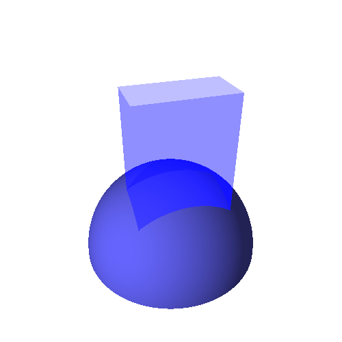
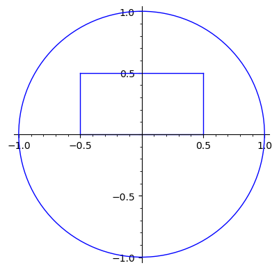
Figure 7: The left image shows the fundamental domain for $\Gamma=\operatorname{PSL}_{2}(\mathbb{Z}[i])$ acting on $\mathcal{H}^{3}$. The longer axis of the rectangle bounding the bottom is the $x_{0}$-axis. The right image is the fundamental domain for $\Gamma_{\infty}$ in $V_{2}$ and the intersection of the sphere defining the bubble domain with $V_{2}$.

10.2.2 Generators

The associated matrices are given by

$$\tau_{1}=\begin{pmatrix}1&1\\ 0&1\end{pmatrix},\quad\tau_{-1}=\begin{pmatrix}1&-1\\ 0&1\end{pmatrix},\quad\gamma_{3}=\begin{pmatrix}i&-1\\ 0&-i\end{pmatrix},\quad\pi_{i}=\begin{pmatrix}i&0\\ 0&-i\end{pmatrix},\quad S=\begin{pmatrix}0&1\\ -1&0\end{pmatrix}.$$

This may be checked by showing that they preserve the respective facets and take points inside the fundamental domain and close to them across the facets.

As before, Corollary 8.3.4 confirms that $\tau_{1}\tau_{-1}=\gamma_{3}^{2}=\pi_{i}^{2}=S^{2}=e$. In addition, the $2$-faces induce the relations

$$(\tau_{1}\gamma_{3})^{2}=(\tau_{1}\pi_{i})^{2}=(\tau_{1}S)^{3}=(\gamma_{3}S)^{3}=(\pi_{i}S)^{2}.$$

In [Sengun2012, Sect. 2.3] we find the presentation

$$\langle a,b,c,d|a^{3},b^{2},c^{3},d^{2},(ac)^{2},(ad)^{2},(bc)^{2},(bd)^{2}\rangle,$$

which is transformed into ours by setting $a=\tau_{1}S,b=S,c=S\gamma_{3},d=S\pi_{i}$.

10.3 The Case of $\mathbb{Q}(\sqrt{-19})$

The case of the class number one field $K=\mathbb{Q}(\sqrt{-19})$ with maximal order $\mathcal{O}=\mathbb{Z}[\omega]$ where $\omega=\frac{1+\sqrt{-19}}{2}$ is a prototypical example of what we want to generalize. We let $\Gamma=\operatorname{PSL}_{2}(\mathcal{O})$.

This is the first example in which there is a sphere whose radius is not equal to $1$. The maximal orders in $\mathbb{Q}(\sqrt{-m})$ for $m=1,2,3,7,11$ are all Euclidean and give rise to simple fundamental domains where all of the balls are centered at integers; likewise with $m=5,6,15$, for which the maximal order has class number $2$. Ordering by discriminant, the first case where the fundamental domain has two balls is $\mathbb{Q}(\sqrt{-7})$. All of these examples were investigated by Bianchi and Swan [Swan1971].

10.3.1 Unit Group and Fundamental Domain for $\Gamma_{\infty}$

The order $\mathcal{O}$ has $\mathcal{O}^{\times}=\{\pm 1\}$, so $\Gamma_{\infty}\cong\operatorname{Vec}(\mathcal{O})=\mathcal{O}$ and the fundamental domain $F$ for the lattice $\Lambda=\operatorname{Vec}(\mathcal{O})$ is then $F=\{x_{0}+ix_{1}\colon-1/2\leq x_{0}\leq 1/2,-\sqrt{19}/4\leq x_{1}\leq\sqrt{19}/4\}.$ The division by $4$ has to do with the congruence of 19 modulo $4$ and the shape of the basis of the $\mathcal{O}$. By symmetry, it is enough to know the basis when $x_{0}\geq 0$ and $x_{1}\geq 0$, and we will often restrict to this case.

10.3.2 Fundamental Domain

In our situation we have elected to show the spheres involved above the set with $-1/2\leq x_{0}\leq 1/2$ and $0\leq x_{1}\leq\sqrt{19}/2$. There are five bubbles involved

$$B(0),\quad B(\omega),\quad B(\omega-1),\quad B(\omega/2),\quad B((\omega-1)/2).$$

The first three bubbles have curvature $1$ (radius $1$)—the base points are elements of $\mathcal{O}$. The bubbles $B(\omega/2),B((\omega-1)/2))$ have curvature $4$ and radius $1/2$. There are two images shown in Figure 8.

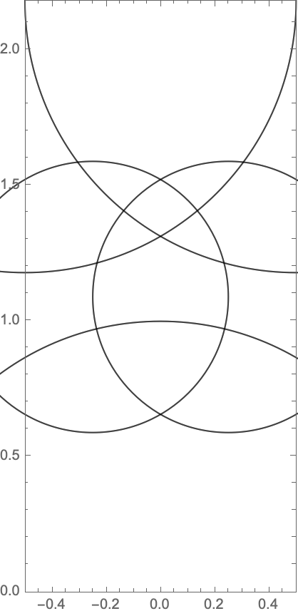
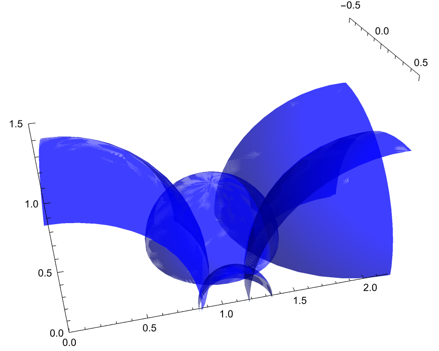
Figure 8: The bubbles of $\mathbb{Q}(\sqrt{-19})$. The above picture shows the five bubbles above the set of $x+iy$ where $-1/2\leq x\leq 1/2$ and $0\leq y\leq\sqrt{19}/2$.

The first shows the traces of the spheres with intersecting the plane $x_{2}=0$, and the other shows a top-down view of this selection of spheres. Note that when two circles intersect, their intersection points determine a line. Along these lines are exactly where the spheres have equal heights. The segments where the two lines intersect are the projections of edges of the fundamental polyhedron—the edge is the edge of the two faces corresponding to the two bubbles.

We remark that all of these cusps are tidy in the sense of §9.5.

11 The Case of $\left(\frac{-1,-1}{\mathbb{Q}}\right)$

For the quaternion algebra $\left(\frac{-1,-1}{\mathbb{Q}}\right)$ we will use the usual quaternion notation with $i_{1}=i$ and $i_{2}=j$ with $ij=k$. We will consider two orders. One is the order $\mathbb{Z}[i,j],$ which is also called the Lipschitz order whose unit group $\mathbb{Z}[i,j]^{\times}$ is isomorphic to $Q_{8}$, the quaternion group of order $8$. We also have the unique maximal order containing it called the Hurwitz Order, which we denote by $\mathcal{O}_{3}=\mathbb{Z}[i,j,\zeta],$ where

$$\zeta=\frac{1+i+j+k}{2}.$$

Note that this makes $\mathcal{O}_{3}\subset\mathbb{C}_{3}\cong\mathbb{R}^{4}$ a $D_{4}$ lattice while $\mathbb{Z}[i,j]$ is just a standard cubic lattice isomorphic to $\mathbb{Z}^{4}$. On the other hand, in both of these cases we have $\operatorname{Vec}(O_{3})=\operatorname{Vec}(\mathbb{Z}[i,j])\cong\mathbb{Z}^{3}$, which is just the standard cubic lattice.

Figure 9: The Dynkin diagram for $\operatorname{Vec}(\mathcal{O}_{3})=\operatorname{Vec}(\mathbb{Z}[i,j])\cong\mathbb{Z}^{3}$.

Proposition 11.0.1.

The Lipschitz order $\mathbb{Z}[i,j]$ and Hurwitz order $\mathcal{O}_{3}$ are Clifford-Euclidean for the norm.

Proof.

In what follows, we let $\mathbb{H}=(-1,-1/\mathbb{Q})$, $\mathbb{L}=(-1,-1/\mathbb{Z})$ and $H=\mathcal{O}_{3}$. Let $\mathbb{H}=H\otimes_{\mathbb{Z}}\mathbb{Q}$ be the Hamilton quaternions. As above, if $xy^{*}\in\operatorname{Vec}(\mathbb{H})$ then $x^{-1}y\in\operatorname{Vec}(\mathbb{H})$. Thus, if $x,y\in\operatorname{Vec}(\mathbb{L})$ with $xy^{*}\in\operatorname{Vec}(\mathbb{L})$, we may write $x^{-1}y=a_{0}+a_{1}i+a_{2}j$. Let the $b_{i}$ be the nearest integers to the $a_{i}$, respectively, and let $c_{i}=a_{i}-b_{i}$; then $x^{-1}y=(b_{0}+b_{1}i+b_{2}j)+(c_{0}+c_{1}i+c_{2}j)$ with $|c_{i}|\leq 1/2$. Multiplying both sides of this equation on the left by $x$ gives the desired expression. ∎

Remark 11.0.2.

It is important to note that $\operatorname{PSL}_{2}(\mathbb{Z}[i,j])$ can have class number 1 without $\mathbb{Z}[i,j]$ being a left principal ideal domain. The point is that, although $\mathbb{Z}[i,j]\cdot(1+i+j+k)+\mathbb{Z}[i,j]\cdot 2$ is not left principal, every cusp of the form $b^{-1}a$ where $a,b$ are Clifford vectors, i.e., of the form $r+si+tj$, is regular.

Lemma 11.0.3.

Let $\mathcal{O}=\mathbb{Z}[i_{1},\ldots,i_{n-1}]$. Let $\Gamma=\operatorname{SL}_{2}(\mathcal{O})$ act on $\mathcal{H}^{n+1}$. The set $F\subset V_{n}$, defined as the set of $x=x_{0}+x_{1}i_{1}+\cdots+x_{n-1}i_{n-1}$ such that

$$-\frac{1}{2}<x_{0}<\frac{1}{2},\qquad 0<x_{j}<\frac{1}{2},\quad 1\leq j\leq n-1,$$

is an open fundamental domain for the action of $\Gamma_{\infty}$ on $V_{n}$.

Proof.

Clearly, $F_{0}=\{x\in V_{n}\colon-1/2<x_{j}<1/2\}$ is an open fundamental domain for $\operatorname{Vec}(\mathcal{O})$. Let $T_{j}(x)=i_{j}xi_{j}$. One has $T_{j}(i_{j})=-i_{j}$, $T_{j}(i_{k})=i_{k}$ for $0<k\neq j$, $T_{j}(1)=-1$. So $T_{j}(x)$ flips the sign of the $x_{0}$ and $x_{j}$ component. The map $T_{j}$ is a $180^{\circ}$ rotation in the $x_{0}x_{j}$-plane. The map $T_{j}$ has any number of fundamental domains in the $x_{0}x_{j}$-plane, but we can choose to always take $x_{0}$ to be long and $x_{j}$ to be short so that $1/2<x_{0}<1/2$ and $0<x_{j}<1/2$. We then intersect all of the fundamental domains for $T_{j}$ to get the result. A picture of the fundamental domain is given in Figure 10.

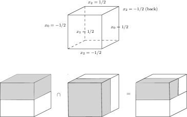
Figure 10: The construction of the fundamental domain for $\operatorname{PSL}_{2}(\mathbb{Z}[i,j])_{\infty}$ in $V_{3}$. Fundamental domains after including $T_{1}$ and $T_{2}$ are included.

∎

11.1 The Case of the Hurwitz Order in $\left(\frac{-1,-1}{\mathbb{Q}}\right)$

There are some standard actions of the Hurwitz order $\mathcal{O}_{3}^{\times}$ that are well-known. For example, this group acts on the tetrahedron embedded in the $i,j,k$ space. We will do something different, acting on the space $V_{3}=\mathbb{R}+i\mathbb{R}+j\mathbb{R}\subset\mathbb{H}$ rather than the usual subspace $\mathbb{R}i+\mathbb{R}j+\mathbb{R}k\subset\mathbb{H}$.

11.1.1 Clifford Units

The Clifford group of units $\mathcal{O}_{3}^{\times}$ has order $24$ and is generated by $i,j$ and $\zeta$, a 6th root of unity:

$$\mathcal{O}_{3}^{\times}=\langle i,j,\zeta\rangle,\quad\zeta=\frac{1+i+j+ij}{2}.$$

Note that while $\zeta$ is a Clifford group element, it can only be written as a product of Clifford vectors from $K=(-1,-1/\mathbb{Q})$ and not $\operatorname{Vec}(\mathcal{O}_{3})$. We have $\zeta=(1+i)(1+j)/2,$ but we can’t write $\zeta$ as a product of elements from $\operatorname{Vec}(\mathcal{O}_{3})\cap\mathcal{O}_{3}^{\times}$. We denote the subgroup generated by $\operatorname{Vec}(\mathcal{O}_{3})\cap\mathcal{O}_{3}^{\times}$ by $\operatorname{Vec}(\mathcal{O}_{3})^{\times}$. This group is just the quaternion group

$$\operatorname{Vec}(\mathcal{O}_{3})^{\times}=Q_{8}=\langle i,j\rangle,$$

and its image in $\operatorname{SO}_{3}(\mathbb{R})\cong\mathcal{O}_{3}^{\times}/\{\pm 1\}$ is the group $C_{2}^{2}$ generated by $\pi_{i}$ and $\pi_{j}$ which act as

$$\pi_{i}(x+yi+zj)=(-x-yi+zj),\quad\pi_{j}(x+yi+zj)=-x+yi-zj.$$

Note that $\operatorname{Vec}(\mathcal{O}_{3})\cong\mathbb{Z}^{3}$, and that this group is actually the subgroup $\operatorname{Weyl}(\mathbb{Z}^{3})^{+}$ of the Weyl group $\operatorname{Weyl}(\mathbb{Z}^{3})$ of the root system $\Phi=\{\pm 1,\pm i,\pm j\}$ in the Euclidean space $V_{3}\cong\mathbb{R}^{3}$ with inner product $\langle x,y\rangle=2x\cdot y$.

Here $C_{2}$ denotes a cyclic group of order 2. See Figure 11 for a picture of the simply laced root system for the root lattice $\mathbb{Z}^{3}$. The full Weyl group would have all of the reflections $r_{1},r_{i},r_{j}$ where $r_{i_{a}}$ reflects the basis element $i_{a}$ and fixes $i_{b}$ for $a\neq b$.

Under the isomorphism $C_{2}^{3}\cong\mathbb{F}_{2}^{3}$ we can view this subgroup of the Weyl group as a code, which is sometimes useful (see e.g. [Dupuy2023, p. 1]). Note that this group-code is not to be confused with our doubly even lattice-codes. The group generated by $\pi_{i}$ and $\pi_{j}$ corresponds to the group generated by $101$ and $110$ in $\mathbb{F}_{2}^{3}$. Here $101$ corresponds to $\pi_{j}$, and $110$ corresponds to $\pi_{i}$.

Figure 11: The Dynkin diagram of $\mathbb{Z}^{3}$

The full quotient $\mathcal{O}_{3}^{\times}/\{\pm 1\}$ is isomorphic to $A_{4}$. We have $A_{4}\cong C_{2}^{2}\rtimes C_{3}$, and indeed the element $\zeta\in\mathcal{O}^{\times}_{3}\setminus\operatorname{Vec}(\mathcal{O}_{3})^{\times}$ comes from an automorphism of the root system $\Phi$ outside of $\operatorname{Weyl}(\Phi)$. The special non-Clifford vector $\zeta=(1+i+j+k)/2$ acts by a cyclic permutation

$$\pi_{\zeta}(x+yi+zj)=z+xi+yj.$$

One sees that $\operatorname{Aut}(\operatorname{Dynkin}(\mathbb{Z}^{3}))=S_{3}$ and $C_{3}=\langle\pi_{\zeta}\rangle\cong A_{3}$, which is the orientation-preserving subgroup of automorphisms of the root system.

11.1.2 Fundamental Domain for $\Gamma_{\infty}$

A fundamental domain for $\Gamma_{\infty}$ is pictured in Figure 12.

Theorem 11.1.1.

The fundamental domain for $\Gamma_{\infty}$ in $V_{3}$ can be described as the collection $F$ of $x+yi+zj$ where $z\in[0,1/2]$ and $0\leq x\leq z$ and $0\leq|y|\leq z$.

Proof.

The space of Clifford vectors is 3-dimensional, and we can translate to make all 3 coordinates have an absolute value less than $1/2$ (uniquely except on the boundary). We break up the positive octant $0\leq x,y,z\leq 1/2$ into 6 pieces depending on the order of $x,y,z$ so one of the pieces is $0\leq y\leq x\leq z\leq 1/2$, etc. We break up the others by taking the image of this triangulation by the Klein four-group maps generated by $\pi_{i_{1}}$ and $\pi_{i_{2}}$. So we have a set of 48 tetrahedra that is preserved by the action of $A_{4}$. The fundamental domain is a set of orbit representatives, ideally one such that the closures meet nicely in facets. One choice is the four tetrahedra:

$$\{0\leq z\leq x\leq y\leq 1/2\},\quad\{0\leq x\leq z\leq y\leq 1/2\}$$

$$\{0\leq-x\leq z\leq y\leq 1/2,x\geq-1/2\}\quad\{0\leq z\leq-x\leq y\leq 1/2,x\geq-1/2\}.$$

One then checks directly that the union of these is precisely the region we have described. ∎

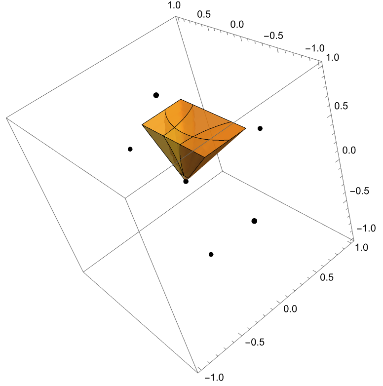
Figure 12: The fundamental domain of $\Gamma_{\infty}$ for $\Gamma=\operatorname{PSL}_{2}(\mathcal{O}_{3})$. Also pictured are the centers of the bubbles $B(0),B(1),B(i),B(-i),B(j),B(-j)$.

11.1.3 Fundamental Domain for $\Gamma$

Theorem 11.1.2.

The fundamental domain for $\operatorname{PSL}_{2}(\mathcal{O}_{3})$ acting on $\mathcal{H}^{4}$ is the region above $F$ with the single bubble $B(0)$.

Proof.

The region $F$ has a convenient description as $|y|\leq z$ and $x\leq z$ for $z\in[0,1/2]$. This is pictured above with centers for the bubbles $B(0),B(1),B(-1),B(i),B(-i),B(j)$. These are the only bubbles that could matter.

The 4-cell bordering $B(0)$ and $B(1)$ sits above a 3-cell in $\{x=1/2\}$ which is on the boundary of $F$. This is the same for the other ones. They project to $\{x=\pm 1/2\}$, $\{y=\pm 1/2\}$ and $\{z=\pm 1/2\}$. None of these are on the interior of $F$ and hence we can omit them.

We will now check the spheres of other radii. First, we consider $B((1+i)/2)$. Since $(1+i)/2=1/(1-i)$ in lowest terms, the radius is $1/\sqrt{2}$. Again, consider a point $(1/2+a,1/2+b,c)$, where $a,b<0$. The point above this in $B(0)$ has fourth coordinate squaring to $1/2-2(a+b)-(a^{2}+b^{2}+c^{2})$, and for $B((1+i)/2)$ it is $1/2-(a^{2}+b^{2}+c^{2})$: also smaller.

After that we need to look at $(1+i+j)/3=1/(1-i-j)$. The radius squared is $1/3$. We have to be more careful, because there is less symmetry. Nevertheless, we claim that a sphere is not needed here. Consider a point lying under this hemisphere whose coordinates are

$$(a+1/3,b+1/3,c+1/3,\sqrt{1/3-(a^{2}+b^{2}+c^{2})}).$$

We first compare to the hemisphere centered at the origin, which includes the point

$$(a+1/3,b+1/3,c+1/3,\sqrt{1-(a+1/3)^{2}+(b+1/3)^{2}+(c+1/3)^{2}}).$$

Squaring the last coordinates and expanding, we have to compare $1/3-(a^{2}+b^{2}+c^{2})$ to $2/3-2/3(a+b+c)-(a^{2}+b^{2}+c^{2})$. After cancelling the square terms, we find that the point on the basic hemisphere centered at $1$ is at least as high if and only if $1/2\geq a+b+c$. This does not follow from the assumption that $a^{2}+b^{2}+c^{2}\leq 1/3$, so as in Algorithm 9.3.2 we consider other hemispheres as well. In particular, with the hemisphere with center $(1,1,1)$ we compare $1/3-(a^{2}+b^{2}+c^{2})$ to

$$1-(2/3-a)^{2}-(2/3-b)^{2}-(2/3-c)^{2}=1-4/3+4/3(a+b+c)-(a^{2}+b^{2}+c^{2}).$$

The right-hand side is greater or equal if and only if $a+b+c\geq 1/2$. Of course, either this condition or the previous condition $1/2\geq a+b+c$ must hold. (In terms of our linear programming, although $1/2\geq a+b+c,a+b+c\geq 1/2$ is a feasible set of inequalities, it is not possible for both of them to hold strictly.) It follows that the hemisphere based at $(1+i+j)/3$ is dominated by the pair of hemispheres with centers $0$ and $1+i+j$. By symmetry it is unnecessary to consider $(\pm 1\pm i\pm j)/3$.

If the denominator has norm 4, the radius is $1/2$. Either the center is one of $1/2,i/2,j/2$ and Lemma 9.3.1 applies with $P=0$ or it is $(\pm 1\pm i\pm j)/2$. It suffices to treat the positive signs; since $(1+i+j)/2$ is in lowest terms the radius is $1/2$. Consider a point $(1/2+a,1/2+b,1/2+c)\in{\mathbb{R}}^{3}$; first, suppose that $a,b,c<0$. Then the fourth coordinate of the point of $B(0)$ above it squares to $1/4-2(a+b+c)-(a^{2}+b^{2}+c^{2})$, and of $B((1+i+j)/2)$ to $1/4-(a^{2}+b^{2}+c^{2})$, which is smaller. Similarly, with a different set of signs we would choose $x,y,z\in\{0,1\}$ such that $x-1/2,y-1/2,z-1/2$ have the same signs as $a,b,c$ and use $B(x+yi+zj)$ in place of $B(0)$.

If the denominator has norm 5, we can take the center to be $(x+yi+zj)/5$ where $5|(x^{2}+y^{2}+z^{2})$ and $x,y,z$ are $0,1,2$. Up to symmetry there is only one possibility, and the distance from $(2+i)/5$ to the origin plus the radius $1/\sqrt{5}$ is less than $1$, so Lemma 9.3.1 applies.

If the denominator has norm 6, the center is $(x+yi+zj)/6$ where $6|(x^{2}+y^{2}+z^{2})$ and $x,y,z\in\{0,1,2,3\}$. We can assume that $(x,y,z)=1$, so essentially the only possibility is $(2+i+j)/6$. Again, Lemma 9.3.1 shows that this sphere is not needed.

If the denominator has norm 7, the center is $(x+yi+zj)/7$ where $7|(x^{2}+y^{2}+z^{2})$ and $x,y,z\in\{0,1,2,3\}$. The only choice is $(3+2i+j)/7$, and again this is taken care of by Lemma 9.3.1.

Finally, we claim that no cusp whose denominator has norm $\geq 8$ can ever be required. Indeed, the distance to the origin is at most $\sqrt{3}/2$, so if the radius is at most $1/\sqrt{n}$ for $n\geq 8$, then distance plus radius is less than $1$ and the hemisphere is dominated by $B(0)$. ∎

11.1.4 Generators

The generators are found using Theorem 9.4.4, where there is a generator for each side of the fundamental domain $D$. They come from the bubbles and the generators of $\operatorname{PSL}_{2}(\mathcal{O}_{3})_{\infty}$. The group $\operatorname{PSL}_{2}(\mathcal{O}_{3})$ is generated by

$$S,\qquad\tau_{1},\quad\tau_{i},\quad\tau_{j},\qquad\pi_{\zeta},\quad\pi_{i},\quad\pi_{j}.$$

11.2 The Case of $\left(\frac{-1,-1}{\mathbb{Z}}\right)$

This was first carried out in [Maclachlan1989, Theorem 8]. A calculation similar to the calculation of the fundamental domain of $\mathbb{Z}[i]$ acting on $\mathcal{H}^{3}$ can be performed for $\mathbb{Z}[i,j]$ acting on $\mathcal{H}^{4}$. The group of units here is the well-known quaternion group

$$\mathbb{Z}[i.j]^{\times}=Q_{8}=\langle\pm 1,\pm i,\pm j,\pm k\rangle.$$

11.2.1 Fundamental Domain

The fundamental domain for $\Gamma^{\prime}=\operatorname{PSL}_{2}(\mathbb{Z}[i,j])$ acting on $\mathcal{H}^{4}$ has as boundaries

$$\{x=-1/2\},\quad\{x=1/2\},\quad\{y=0\},\quad\{y=1/2\}$$

$$\{z=0\},\quad\{z=1/2\},\quad B(0)=\{|x|=1\}.$$

Note that we don’t include $B(1)$ and $B(-1)$ (or other translates by the cubic lattice) because they meet $B(1)$ at $x=1/2$ and $x=-1/2$, respectively. The image of the fundamental domain for $\Gamma_{\infty}$ acting on $V_{3}$ was already pictured in Figure 10.

Remark 11.2.1.

This example is deceptively simple. The same naive example in higher dimensions becomes wildly complicated. We cannot expect the domain bounded by $|x_{i}|\leq 1/2$ and $\sum_{i=1}^{n}x_{i}^{2}+y^{2}=1$ to be fundamental for $n>4$, because it is possible for $\sum_{i=1}^{n}x_{i}^{2}$ to be greater than $1$. Thus we would not expect a set of generators analogous to those above to be sufficient to generate $\operatorname{PSL}_{2}(\mathbb{Z}[i_{1},i_{2},i_{3}])$.

11.2.2 Generators

The generators for $\operatorname{PSL}_{2}(\mathbb{Z}[i,j])$ are the matrices

$$\tau_{1}=\begin{pmatrix}1&1\\ 0&1\\ \end{pmatrix},\tau_{1}^{-1}=\begin{pmatrix}1&-1\\ 0&1\\ \end{pmatrix},\gamma_{3}=\begin{pmatrix}i&-1\\ 0&-i\\ \end{pmatrix},\gamma_{4}=\begin{pmatrix}i&0\\ 0&-i\\ \end{pmatrix},$$

$$\gamma_{5}=\begin{pmatrix}j&-1\\ 0&-j\\ \end{pmatrix},\pi_{j}=\begin{pmatrix}j&0\\ 0&-j\\ \end{pmatrix},S=\begin{pmatrix}0&1\\ -1&0\\ \end{pmatrix}.$$

The relations, which we computed using our algorithm, are rather complicated but given by

$$\tau_{1}\gamma_{3}\tau_{1}\gamma_{3}=1 \tau_{1}\pi_{i}\tau_{1}\pi_{i}=1 \tau_{1}\gamma_{5}\tau_{1}\gamma_{5}=1$$

$$\tau_{1}\pi_{j}\tau_{1}\pi_{j}=1 \tau_{1}S\tau_{1}S\tau_{1}S=1 \tau_{1}^{-1}\gamma_{3}\tau_{1}^{-1}\gamma_{3}=1$$

$$\tau_{1}^{-1}\pi_{i}\tau_{1}^{-1}\pi_{i}=1 \tau_{1}^{-1}\gamma_{5}\tau_{1}^{-1}\gamma_{5}=1 \tau_{1}^{-1}\pi_{j}\tau_{1}^{-1}\pi_{j}=1$$

$$\tau_{1}^{-1}S\tau_{1}^{-1}S\tau_{1}^{-1}S=1 \gamma_{3}\gamma_{5}\gamma_{3}\gamma_{5}=1 \gamma_{3}\pi_{j}\gamma_{3}\pi_{j}=1$$

$$\gamma_{3}S\gamma_{3}S\gamma_{3}S=1 \pi_{i}\gamma_{5}\pi_{i}\gamma_{5}=1 \pi_{i}\pi_{j}\pi_{i}\pi_{j}=1$$

$$\pi_{i}S\pi_{i}S=1 \gamma_{5}S\gamma_{5}S\gamma_{5}S=1 \pi_{j}S\pi_{j}S=1.$$

Note that this implies that Kraußhar’s groups in [Krausshar2004], which are generated by translations $\tau_{i_{a}}$ for $0\leq a\leq n-1$ and $S$, are not $\operatorname{PSL}_{2}(\mathbb{Z}[i_{1},i_{2},\ldots,i_{n-1}])$.

12 The Case of $\left(\frac{-1,-3}{\mathbb{Q}}\right)$

We will view $\left(\frac{-1,-3}{\mathbb{Q}}\right)$ as sitting inside Hamilton’s quaternions, and so $\left(\frac{-1,-3}{\mathbb{Q}}\right)=\mathbb{Q}[i,\sqrt{3}j]$. Inside $\left(\frac{-1,-3}{\mathbb{Q}}\right)$ there are two maximal orders $\mathcal{O}(-1,-3)_{1}$ and $\mathcal{O}(-1,-3)_{2}$ which contain the elements $(1+\sqrt{3}j)/2$ and $(1+\sqrt{3}k)/2$, respectively. Note that one has a third root of unity which is a Clifford vector while the other does not. These orders are conjugate to each other by $1+i$. Also observe that we cannot generate a single order with both roots of unity in it, because $(1+\sqrt{3}j)/2-(1+\sqrt{3}k)/2$ is not integral; it has minimal polynomial $x^{2}+3/2$.

12.1 The Case of $\mathcal{O}(-1,-3)_{2}$

We will work with $\mathcal{O}=\mathcal{O}(-1,-3)_{2}.$ Everything is the same for $\mathcal{O}(-1,-3)_{1}$, since it is conjugate to this one by a Clifford vector. This order contains the elements

$$\zeta=\frac{1+\sqrt{3}k}{2},\quad\zeta^{6}=1,\qquad J=\frac{i+\sqrt{3}j}{2},\quad J^{2}=-1.$$

The element $J$ may appear strange, since it acts like $\sqrt{-1}$ but looks like a primitive 6th root of unity in the $yz$-plane. After running our algorithm for finding bubbles above the region with

$$\Omega=\{x+iy+jz\colon-1/2\leq x,y\leq 1/2,\sqrt{3}/2\leq z\leq 1/2\}$$

we found three potential spheres,

$$B(0),\quad B(J),\quad B(J-i).$$

By symmetry we plotted these in Figure 13 (see the caption). We will reduce the size of the region $\Omega$ and show that only $B(0)$ is actually needed.

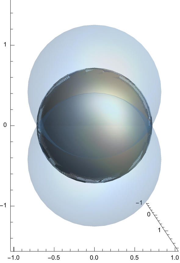
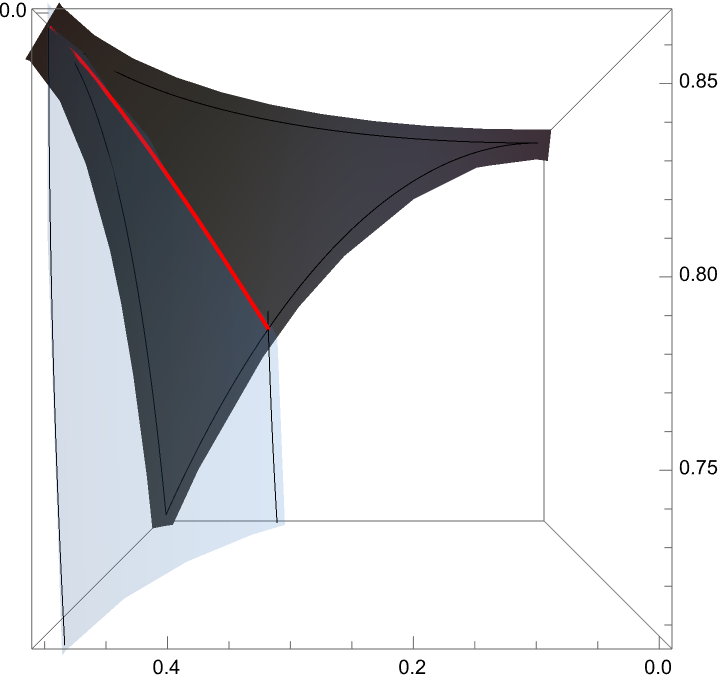
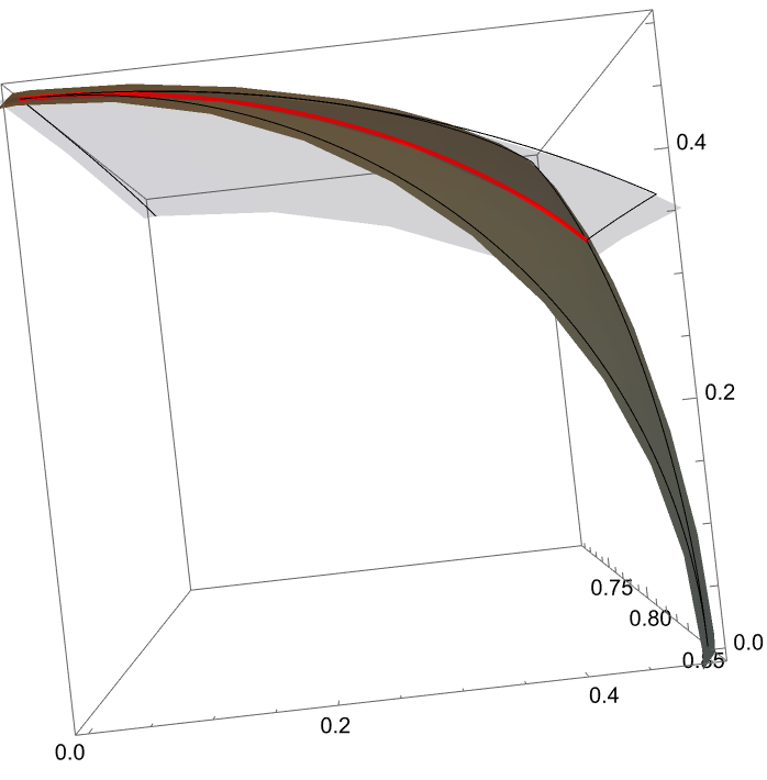
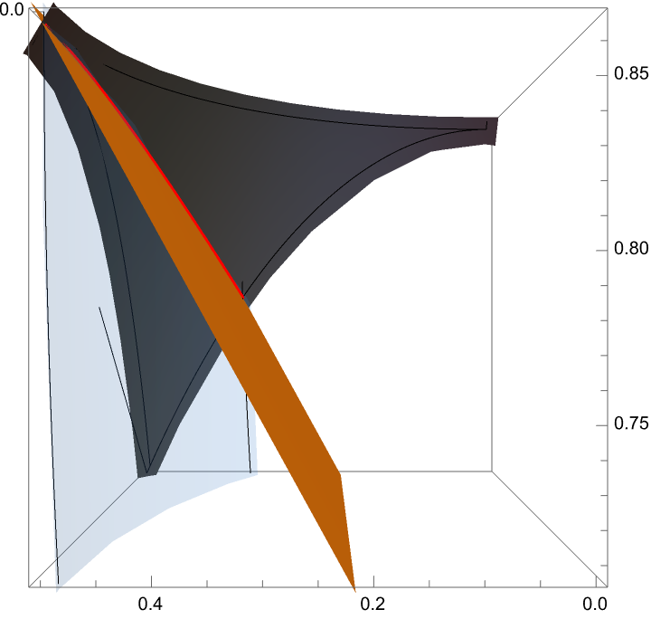
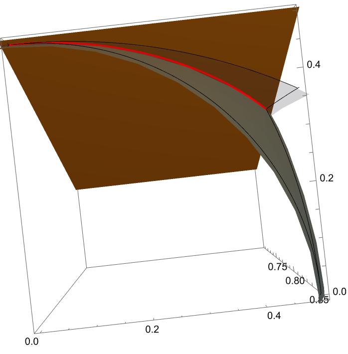
Figure 13: The first row shows the collection of spheres that are above to the region with $-1/2\leq x_{j}\leq 1/2$. The three potential spheres $B(0),B(\frac{i_{1}+\sqrt{3}i_{2}}{2})$, and $B(\frac{-i_{1}+\sqrt{3}i_{2}}{2})$ are to be used as bubbles for the maximal order of $\left(\frac{-1,-3}{\mathbb{Q}}\right)$ where $\partial\mathcal{H}^{4}=V_{3}$. These spheres are pictured from the front, left, and top, respectively, in each column. On the second and third rows we restrict to the region of $x=x_{0}+i_{1}x_{1}+\sqrt{3}i_{2}x_{2}$ with $0\leq x_{j}\leq 1/2$ (so the fundamental domain of $\Gamma_{\infty}$ is not included in this picture). The middle row shows the where the sphere $B(\frac{i_{1}+\sqrt{3}i_{2}}{2})$ intersects $B(1)$ in a red arc. The bottom row displays the plane containing the red line. There is a region in $V_{3}$ in this plane containing the red line on the interior of both spheres where the height of $B(0)$ and $B(\frac{i_{1}+\sqrt{3}i_{2}}{2})$ in $\mathcal{H}^{4}$ are equal. This is analogous to the chord determined by two circles—along this finite chord the two spheres sitting above the circles in the plane will have the same height. Note the radial symmetry in the picture from the left (middle column) where the $x_{1}x_{2}$-axis is easier to see.

12.1.1 Unit Group

The Clifford unit group of $\mathcal{O}^{\times}$ is given by

$$\mathcal{O}^{\times}=\{\pm 1,\frac{\pm 1\pm\sqrt{3}k}{2},\frac{\pm i\pm\sqrt{3}j}{2},\pm i\}=\langle\zeta,J\rangle.$$

This group is generated by $\zeta$ and $J$, which have order $6$ and $4$, respectively. The elements $J$, $J\zeta$, and $\zeta J$ are all square roots of $-1$ and $J\zeta=i$. There are $1,1,4,4,2$ units of order $1,2,3,4,6$, respectively.

The group modulo $\{\pm 1\}$, which acts by conjugation, also has a nice description:

$$\mathcal{O}^{\times}/\{\pm 1\}=\langle\overline{\zeta},\overline{J}\rangle\cong D_{3}.$$

Note that $\zeta J\zeta J=-1$ implies that $\mathcal{O}^{\times}/\{\pm 1\}\cong D_{3}$ with generators $\overline{\zeta}$ and $\overline{J}$.

12.1.2 Fundamental Domain for $\Gamma_{\infty}$

For $a\in V_{3}$ the map $\pi_{\zeta}(a)=\zeta a\zeta^{*}$ acts like a $2\pi/3$-rotation in the $yz$-plane and acts trivially in the $x$-plane. The map $\pi_{J}$ is given by

$$\pi_{J}(1)=-1,\quad\pi_{J}(i)=i/2-\sqrt{3}j/2,\quad\pi_{J}(j)=-\sqrt{3}i/2-j/2.$$

This is the reflection in the $yz$-plane across the line $y+\sqrt{3}z=0$ with a change in sign in the $x$-coordinate. Note that this sign change in the $x$-axis converts the reflection into an orientation-preserving map, which can be thought of as a rotation (as usual, the compositum of two reflections is a rotation).

One can see that the representation $\pi:D_{3}=\mathcal{O}^{\times}/\{\pm 1\}$ is reducible with $\mathbb{R}\subset V_{3}$ being just the sign and $D_{3}$ acting on $\mathbb{R}i+\mathbb{R}j\subset V_{3}$ via the usual dihedral action.

The fundamental domain in the $yi+zj$-plane is pictured in Figure 14. This was found with a little trial and error and came from modifying a Dirichlet domain for $\operatorname{Im}(\operatorname{Vec}(\mathcal{O}))$ to be invariant under the $D_{3}$ action. If we let $H_{12}$ be the inner honeycomb in Figure 14, which is not the fundamental domain, we can construct the “Allen wrench”

$$A=[-1/2,1/2]\times H_{12},$$

and observe that the Allen wrench is a fundamental domain for $\operatorname{Vec}(\mathcal{O})$. It is also invariant under the dihedral action with reflections turning around the Allen wrench. Then the wedge of the honeycomb (or “orange slice”) $W$, pictured with the fat lines in the stained glass picture (Figure 14) together with half of the extrusion, gives the fundamental domain for $\Gamma_{\infty}$,

$$F=]0,1/2[\times W.$$

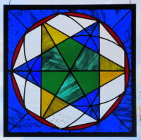
Figure 14: Left: The $yz$-plane cross section of the orbits of the fundamental domain for the action of $\operatorname{SL}_{2}(\mathcal{O}(-1,-3)_{2})_{\infty}$. A fundamental domain is the union of two triangles highlighted with fat lines. Right: Enneagon Inscribed in a Circle by Paul Powers of Power Squared Gallery in Santa Fe, New Mexico. An image of the stained glass piece is reproduced here with the artist’s permission. The symmetry of the stained glass piece is closely related to that of $\operatorname{SL}_{2}(\mathcal{O}(-1,-3)_{2})_{\infty}$. https://powersquaredglassworks.com/gallery.

12.1.3 Fundamental Domain for $\Gamma$

The open fundamental domain for $\operatorname{PSL}_{2}(\mathcal{O}(-1,-3)_{2})$ acting on $\mathcal{H}^{4}$ is

$$D=\{x+i_{1}y+i_{2}z+i_{3}w\colon|x+i_{1}y+i_{2}z+i_{3}w|\geq 1,x+i_{1}y+i_{2}z\in F\}.$$

We are claiming that the only bubble that resulted from our initial computation that actually is used is $B(1)$. The bubbles $B(J)$ and $B(1)$ meet at $J/2$, and the slice of the fundamental domain for $\Gamma_{\infty}$ in $V_{3}$ in the $yz$-plane is above $H_{12}$. It is a convex polytope with a vertex at $J/2$, so the projection of the wall where the sides associated to $B(0)$ and $B(J)$ meet projects to something which only intersects this fundamental domain at the boundary.

More precisely, the wall in the bottom row of Figure 13 contains the long side $A$ which meets $J$. In particular, it meets the long side of $A$ there as well. So we do not need $B(J)$, but only by the skin of our teeth.

12.1.4 Generators

The generators are found using Theorem 9.4.4. The group $\operatorname{SL}_{2}(\mathcal{O})$ is generated by

$$S=\begin{pmatrix}0&-1\\ 1&0\end{pmatrix},\ \tau_{J}=\begin{pmatrix}1&J\\ 0&1\end{pmatrix},\ \tau_{i}=\begin{pmatrix}1&i\\ 0&1\end{pmatrix},\ \tau_{1}=\begin{pmatrix}1&1\\ 0&1\end{pmatrix},\ \pi_{\zeta}=\begin{pmatrix}\zeta&0\\ 0&\zeta\end{pmatrix},\ \pi_{J}=\begin{pmatrix}J&0\\ 0&-J\end{pmatrix}.$$

The generator $S$ is for the bubble $B(0)$, the generators $\tau_{J},\tau_{i},\tau_{1}$ are for the walls corresponding to $\operatorname{Vec}(\mathcal{O})$, and $\pi_{\zeta}$ and $\pi_{J}$ are the extra symmetries for the other walls corresponding to vertices of $F$. Concretely, let the fundamental domain depicted in Figure 14 be $F_{0}$, and for $i\in\mathbb{Z}/6\mathbb{Z}$ let $F_{i}$ be its counterclockwise rotation by an angle of $2\pi i/6$. Then $\pi_{\zeta}(F_{i})=F_{i+2}$, while $\pi_{J}(F_{i})=F_{3-i}$. In particular, the matrices $\pi_{\zeta}\pi_{J}$ and $\pi_{J}\pi_{\zeta}$ give reflections across two of the thick black boundary walls of $F_{0}$; for the third we may use the composition of $\pi_{J}$ with translation by $J$. One readily checks that $\langle\pi_{\zeta},\pi_{J}\rangle=\langle\pi_{\zeta}\pi_{J},\pi_{J}\pi_{\zeta}\rangle$, establishing the correctness of the given set of generators. In fact, we do not need $\tau_{i}$, since it does not correspond to any wall of the fundamental domain. A more basic set of generators would be $\tau_{1},\pi_{J}\pi_{\zeta},\pi_{\zeta}\pi_{J},\tau_{J}\pi_{J},S$. (The fundamental domain has six walls, but $\tau_{1}^{-1}$, which crosses the wall at $x=-1/2$, may be omitted, since $\tau_{1}$ is already present. As expected, we can express $\tau_{i}$ in terms of these generators: it is $(\tau_{J}\pi_{J})(\pi_{\zeta}\pi_{J})(\tau_{j}\pi_{J})(\pi_{J}\pi_{\zeta})$.)

Relations arise from pairs of intersecting walls of the fundamental domain as in Section 8.3. Thus the product of $\tau_{1}$ with any of $\pi_{J}\pi_{\zeta},\pi_{\zeta}\pi_{J},\tau_{J}\pi_{J}$, or of $\pi_{J}\pi_{\zeta}$ or $\pi_{\zeta}\pi_{J}$ with $S$, has order $2$; the product of any two of $\pi_{J}\pi_{\zeta},\pi_{\zeta}\pi_{J},\tau_{J}\pi_{J}$ has order $3$; and likewise $(\tau_{1}S)^{3}=(\tau_{J}\pi_{J}S)^{3}=1$, and these are all of the relations.

Finally, we remark that for $\mathcal{O}=\left(\frac{-1,-3}{\mathbb{Z}}\right)$, the analogue of the Lipschitz order in this context, the group $\operatorname{SL}_{2}(\mathcal{O})$ has index $15$ in $\operatorname{SL}_{2}(\mathcal{O}(-1,-3))$. This can be proved by Proposition 9.6.1 or directly from the presentation.

13 The Case of $\left(\frac{-1,-1,-1}{\mathbb{Q}}\right)$

By computation, the integral Clifford algebra $\mathbb{Z}[i_{1},i_{2},i_{3}]$ is contained in a unique maximal order $\mathcal{O}_{4}$. The order $\mathcal{O}_{4}$ is generated over $\mathbb{Z}[i_{1},i_{2},i_{3}]$ as an associative algebra by the elements $(1+i_{123})/2$ and $\zeta=(1+i_{1}+i_{2}+i_{3})/2$. Thus the code associated to this order is spanned by $1111$. However, the order $\mathcal{O}_{4}$ is not generated by any single element over $\mathbb{Z}[i_{1},i_{2},i_{3}]$: to prove this, it suffices to consider one representative for each coset of the additive group $\mathcal{O}_{4}/\mathbb{Z}[i_{1},i_{2},i_{3}]$, whose order is $64$. It is generated by $(1+i_{123})/2$ and $(1+i_{1}+i_{2}+i_{12})/2$.

The lattice $\Lambda=\operatorname{Vec}(\mathcal{O}_{4})$ is $\frac{1}{2}\Lambda_{C}$, which is a nonstandard presentation of the checkerboard lattice $D_{4}$. This is the analog of the Hurwitz quaternions.

We remind the reader that the $D_{4}$ lattice in our presentation also has an $F_{4}$ root system; root lattices with short and long vectors can have two distinct root systems, and furthermore such lattices can be root lattices for both root systems. The ADE lattices are classified by their simply laced Dynkin diagrams (no double arrows), which in this case is $D_{4}$.

13.1 The case of the unique maximal order $\mathcal{O}_{4}$ in $\left(\frac{-1,-1,-1}{\mathbb{Q}}\right)$

This is an example where $\operatorname{PSL}_{2}(\mathcal{O}_{4})_{\infty}$ is very interesting but the bubbles are not so interesting. The order $\mathcal{O}_{4}$ is our example of a Clifford-Euclidean order which is not Clifford-principal (meaning that one can perform the Euclidean algorithm for unimodular pairs).

Theorem 13.1.1.

The order $\mathcal{O}_{4}$ is Clifford-Euclidean but not Clifford-principal.

Proof.

It follows from Theorem 3.6.2 that $\mathcal{O}_{4}$ is Clifford-Euclidean. On the other hand, we claim that $\mathcal{O}_{4}$ is not Clifford-principal. Indeed, let $a=(-3+i_{1}+i_{2}-i_{3})(i_{1}),b=(-2-i_{1}-i_{3})(1+i_{1})$: both belong to $\mathcal{O}_{4}^{\vartriangleright}$. The index in $\mathcal{O}_{4}$ of the right ideal $aR+bR$ is $9\cdot 4^{4}$, which is not a fourth power. Therefore, this ideal is not generated by an element of $\mathcal{O}_{4}^{\vartriangleright}$. ∎

Let $\Gamma=\operatorname{PSL}_{2}(\mathcal{O}_{4})$. The fundamental domain is clearly contained in the fundamental domain $F^{\prime}$ for $\Gamma^{\prime}_{\infty}$ where $\Gamma^{\prime}=\operatorname{PSL}_{2}(\mathbb{Z}[i_{1},i_{2},i_{3}])$, which has three 180-degree rotations in the $x_{0}x_{1}$, $x_{0}x_{2}$ and $x_{0}x_{3}$ planes giving

$$-\frac{1}{2}\leq x_{0}\leq\frac{1}{2},\quad 0\leq x_{1}\leq\frac{1}{2},\quad 0\leq x_{2}\leq\frac{1}{2},\quad 0\leq x_{3}\leq\frac{1}{2}.$$

We can figure out which spheres lie over $F^{\prime}$.

Lemma 13.1.2.

Suppose that $a=\mu^{-1}\lambda=a_{0}+a_{1}i_{1}+a_{2}i_{2}+a_{3}i_{3}\in K$ with $0\leq a_{j}\leq 1/2$ with $(\mu,\lambda)$ unimodular. Then $B(a)$ is completely contained in $B(0)$ or $B(\zeta)$.

Proof.

We can suppose that $|\mu|^{2}\geq 2$ without loss of generality. For a hemisphere of radius $r_{1}$ at $x_{1}$ to cover a hemisphere of radius $r_{2}$ at $x_{2}$ we need to show that $|x_{1}-x_{2}|+r_{2}\leq r_{1}$. The sphere in question has radius $r_{2}=1/\sqrt{2}$.

Suppose this is false. Then we need both $|0-a|+1/|\mu|>1$ and $|\zeta-a|+1/|\mu|>1$. This implies that $|a|>1-1/\sqrt{2}$ and $|\zeta-a|>1-1/\sqrt{2}$. Lemma 9.2.1 shows that $|a|\leq 1$ or $a=\zeta$, so not both of the equalities in the previous sentence can hold. ∎

Remark 13.1.3.

In the case of $\operatorname{PSL}_{2}(\mathbb{Z}[i_{1},i_{2},i_{3}])$ the element $\zeta$ will now be a deep hole for the lattice and is a singular cusp. We cannot place a sphere there. We deal with this in §13.3.

13.1.1 Unit Group

The group of units has order $576$ and is given by

$$O_{4}^{\times}=\langle i_{1},i_{2},i_{3},\zeta,\alpha\rangle,\qquad\zeta=\frac{1+i_{1}+i_{2}+i_{3}}{2},\quad\alpha=\frac{i_{1}-i_{12}-i_{23}-i_{31}}{2}.$$

The subgroup $Q_{16}=\langle i_{1},i_{2},i_{3}\rangle$ has order 16, and the maps $\pi_{i_{a}}$ act by $\pi_{i_{a}}(1)=-1$, $\pi_{i_{a}}(i_{a})=-i_{a}$, $\pi_{i_{a}}(i_{b})=i_{b}$, and should be viewed as a rotation of angle $\pi$ in the $x_{0}x_{a}$-plane. The subgroup $\operatorname{Vec}(\mathcal{O}_{3})^{\times}$, defined to be the group generated by Clifford group elements which also happen to be elements of $\operatorname{Vec}(\mathcal{O}_{3})^{\times}$, is $\langle i_{1},i_{2},i_{3},\zeta\rangle$, which has order $192$. The group $\{\pi_{v}\colon v\in\operatorname{Vec}(\mathcal{O}_{3})\}\cong\operatorname{Vec}(\mathcal{O}_{3})^{\times}/\{\pm 1\}$ that describes the action of the integral vectors that are Clifford units on the space of Clifford vectors has order $96$ and is a subgroup of the positive orientation Weyl group $\operatorname{Weyl}(D_{4})^{+}$, which has index two in $\operatorname{Weyl}(D_{4})$ (these are the transformations that have determinant $1$). The Weyl group of $D_{4}$ is isomorphic to $C_{2}^{3}\rtimes S_{4}$ (in general $\operatorname{Weyl}(D_{n})$ is $C_{2}^{n-1}\rtimes S_{n}$ where $S_{n}$ permutes the factors and $C_{2}^{n-1}$ is viewed as an $n-1$-dimensional $\mathbb{F}_{2}$-vector subspace of $\mathbb{F}_{2}^{n}$ ) and $\operatorname{Weyl}(D_{n})^{+}\cong C_{2}^{3}\rtimes A_{4}$. Since $96=2^{3}\cdot(4!/2)$, it follows that

$$\langle\pi_{i_{1}},\pi_{i_{2}},\pi_{i_{3}},\pi_{\zeta}\rangle=\operatorname{Weyl}(D_{4})^{+},$$ (50)

with the elements $\pi_{i_{1}},\pi_{i_{2}},\pi_{i_{3}}$ being the three generators of $C_{2}^{3}$ and $\pi_{\zeta}$ acting as a rotation by an angle of $2\pi/3$.

The quotient group $\mathcal{O}^{\times}/\{\pm 1\}$ has order $576/2=288=3\cdot 96$. The element $\pi_{\alpha}$ acts as a cyclic permutation of $i_{1},i_{2},i_{3}$, and this is actually an automorphism of the Dynkin diagram (so an automorphism of the root system which isn’t in the group generated by reflections in the roots). One has $\operatorname{Aut}(\operatorname{Dynkin}(D_{4}))=S_{3}$ (see Figure 15); this has to do with the famous triality automorphism of $\operatorname{SO}_{8}$.

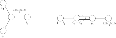
Figure 15: The lattice $\operatorname{Vec}(\mathcal{O}_{4})$ is a root lattice for both $D_{4}$ and $F_{4}$ root systems. Left: the Dynkin graph for the simply laced root system of $D_{4}$ as modeled in $\operatorname{Vec}(\mathcal{O}_{4})$. All the vectors here are short, and all the angles of intersection of elements of the root system are the same. Right: The Dynkin diagram for the root system $F_{4}$.

This element of order $3$ describes $\mathcal{O}_{4}^{\times}/\{\pm 1\}$ as an extension of $\operatorname{Weyl}(D_{4})^{+}$ by $C_{3}$, so rather than an action on just $D_{4}$, it is perhaps best to think about this as a representation to $\operatorname{Aut}(\Phi)$ where $\Phi$ is the root system. The group $\operatorname{Weyl}(F_{4})$ has order $1152$, which is $4\cdot 288$. We now explain how $288$ arises as the order of $\mathcal{O}^{\times}_{4}/\{\pm 1\}$.

The $D_{4}$-lattice $\operatorname{Vec}(\mathcal{O}_{4})$ also has an $F_{4}$-root system. Now, when we speak of $D_{4}$ we will speak of the root system $\Phi_{0}\subset\operatorname{Vec}(\mathcal{O}_{4})$ of this lattice and not the lattice itself. The $D_{4}$-root system is given by $\pm$ coordinate vectors and all vectors with entries $\pm 1/2$, so $24$ in all. The $F_{4}$-root system is the $D_{4}$-root system together with all vectors with two entries $0$ and two $\pm 1$.

We have $\operatorname{Aut}(D_{4})=\operatorname{Aut}(F_{4})=\operatorname{Weyl}(F_{4})$, which we will just call $G$. This is a Schläfli group and hence is the symmetry group of a polytope in $C_{24}$ (see §13.2). We have $\operatorname{Weyl}(D_{4})\subset\operatorname{Aut}(D_{4})$ being a normal subgroup generated by reflections, and $\operatorname{Aut}(\Phi)/\operatorname{Weyl}(\Phi)$ is the set of graph automorphisms of the Dynkin diagram for the $D_{4}$-root system (Figure 15). This is the group $S_{3}$. This means the triality map $\pi_{\alpha}$ is actually in $\operatorname{Weyl}(F_{4})^{+}$, which implies that the fundamental domain for $\Gamma_{\infty}$ in $V_{4}$ is four translates of the “higher-dimensional platonic solid” $C_{24}$ pasted together.

13.2 Coxeter Groups and Classification of Polyhedra

In this section, we give a brief introduction to Coxeter groups and their relation to the classification of polyhedra. The reader unfamiliar with Coxeter groups may wish to consult a standard reference such as [BB2005]. Here we only state a few basic definitions and results.

A Coxeter group [BB2005, 1.1] is a pair consisting of a group $G$ and a set of involutions $S=\{s_{1},\dots,s_{n}\}$ that generate $G$, such that the relations are all of the form $(s_{i}s_{j})^{m_{ij}}=1$. Given a Coxeter group, the associated Coxeter diagram or Coxeter graph is the graph whose vertex set is in bijection with $S$ and that has an edge labeled $m_{ij}$ between $v_{i}$ and $v_{j}$ if $m_{ij}>2$.

In particular, two vertices are adjacent if and only if the corresponding generators do not commute. Every group of isometries of $\mathbb{R}^{n}$ or $\mathcal{H}^{n}$ generated by reflections is a Coxeter group, so the distinguished generators are often called reflections.

A Schläfli symbol is a sequence $\{m_{0,1},m_{1,2},m_{2,3},\ldots,m_{n-1,n}\}$ of integers $\geq 3$ that encodes a Coxeter group with generators $s_{0},\ldots,s_{n}$ and relations $(s_{i}s_{i+1})^{m_{i,i+1}}=1$ for $i=0,1,\ldots,n-1$ and $(s_{i}s_{j})^{2}=1$ for $|i-j|>1$. For example, the symbol $\{3,4,3\}$ is the group generated by $s_{0},s_{1},s_{2},s_{3}$ where

$$(s_{0}s_{1})^{3}=(s_{1}s_{2})^{4}=(s_{2}s_{3})^{3}=(s_{0}s_{2})^{2}=(s_{0}s_{3})^{2}=(s_{1}s_{2})^{2}=1.$$

Schläfli symbols are in bijection with Coxeter diagrams whose underlying graph is a path.

Theorem 13.2.1.

The isometry group of a regular polyhedron $P$ is a Coxeter group whose underlying graph is a path (and can hence be described by a Schläfli symbol). Regular polyhedra up to similarity and duality are classified by their associated isometry group.

13.2.1 Fundamental Domain for $\Gamma_{\infty}$

In what follows we make use of the bijection between polyhedra and their Coxeter group. See §13.2. The 24-cell is the unique polyhedron with Schläfli symbol $\{3,4,3\}.$ Its isometry group is $\operatorname{Weyl}(F_{4})$. The 24-cell also goes by the names icositetrachoron, octaplex, icosatetrahedroid, octacube, hyperdiamond or polyoctahedron.

Theorem 13.2.2.

The fundamental domain for $\operatorname{PSL}_{2}(\mathcal{O}_{4})_{\infty}$ acting on $V_{4}$ is a union of four translates of the 24-cell.

Proof.

The group polyhedron $C_{24}$ is a fundamental domain for the action of $\operatorname{Weyl}(F_{4})$ on the cube $[-1/2,1/2]^{4}\subset V_{4}$. Let $U$ be the image of $\pi:\mathcal{O}_{4}^{\times}/\{\pm 1\}\to\operatorname{GL}(V_{4})$ given by $\pi_{u}(x)=uxu^{*}$. We showed via a magma computation that $U$ has index $4$ in $\operatorname{Weyl}(F_{4})$.

The group $U$ intersects the group of signed permutation matrices in a subgroup of order $96$ (as before, we can apply an even permutation to the coordinates and independently change the sign of an even number of them). However, elements of the unit group like $\zeta=(1+i_{1}+i_{2}+i_{3})/2$ give matrices that act in a more complicated way. One can check that this group of order $288$ is a subgroup of the Coxeter group $\operatorname{Weyl}(F_{4})$. We can extend this group by the diagonal matrix $\operatorname{diag}(1,1,1,-1)$ and the permutation matrix $(3,4)$. These together with $U$ generate a group isomorphic to $\operatorname{Weyl}(F_{4})$. So if we can write down a fundamental domain for the action of $\operatorname{Weyl}(F_{4})$ on the face-centered unit cube $[-1/2,1/2]^{4}$, then the union of the translates by coset representatives for $U$ in $\operatorname{Weyl}(F_{4})$ will be a fundamental domain for $U$. In particular we may take the identity, the two elements $\operatorname{diag}(1,1,1,-1)$ and $(3,4)$ mentioned above, and their product. ∎

A fundamental domain for the group of signed permutations of order 384, which is the Weyl group $\operatorname{Weyl}(B_{4})$ acting on the unit cube centered at $0$, is the subset

$$\{(a,b,c,d)\colon 0\leq d\leq c\leq b\leq a\leq 1/2\}.$$

Our group is an extension of this, and all the rows of elements of our group either have one $\pm 1$ and three $0$ entries or all four entries $\pm 1/2$. Knowing the inequalities just given, we can determine all inequalities formed by dot products with vectors of $\pm 1$ except for two. For example, we know that $a+c\geq b+d$; however, the inequalities $a+d\geq b+c$ and $a\geq b+c+d$ are undetermined.

Lemma 13.2.3.

The locus $L$ defined by

$$L=\{(a,b,c,d)\colon 0\leq d\leq c\leq b\leq a\leq 1/2,a\geq b+c+d\}$$

is a fundamental domain for $\operatorname{Weyl}(F_{4})$ on $[-1/2,1/2]^{4}\subset V_{4}$.

Proof.

Consider the matrices

$$T_{1}=\begin{pmatrix}\frac{1}{2}&\frac{1}{2}&\frac{1}{2}&\frac{1}{2}\\ \frac{1}{2}&\frac{1}{2}&-\frac{1}{2}&-\frac{1}{2}\\ \frac{1}{2}&-\frac{1}{2}&\frac{1}{2}&-\frac{1}{2}\\ -\frac{1}{2}&\frac{1}{2}&\frac{1}{2}&-\frac{1}{2}\end{pmatrix},\qquad T_{2}=\begin{pmatrix}\frac{1}{2}&\frac{1}{2}&\frac{1}{2}&\frac{1}{2}\\ \frac{1}{2}&\frac{1}{2}&-\frac{1}{2}&-\frac{1}{2}\\ \frac{1}{2}&-\frac{1}{2}&\frac{1}{2}&-\frac{1}{2}\\ \frac{1}{2}&-\frac{1}{2}&-\frac{1}{2}&\frac{1}{2}\end{pmatrix},$$

which we view as maps on $(a,b,c,d)$ acting on the right.

If $v=(x,y,z,w)$ is in $L$, then its images by both of these belong to

$$\{(a,b,c,d):0\leq d\leq c\leq b\leq a\leq 1/2\}.$$

For example, $(vT_{1})_{2}-(vT_{1})_{3}=y-z\geq 0$, and $(vT_{2})_{1}=(x+y+z+w)/2\leq x\leq 1/2$. In addition, $vT_{2}$ satisfies $a+d\geq b+c$ but not $a\geq b+c+d$, while $vT_{1}$ satisfies neither of these inequalities. So if $v$ is any vector in the positive orthant, then either it is in $L$ or multiplying it by the inverse of one of these matrices puts it in $L$. Thus, since this is a transversal for the signed permutation group, every $v$ in the cube can be put in the interior of $L$ by a unique element of $W(F_{4})$, except for boundary points in a set of measure $0$. ∎

Corollary 13.2.4.

Let $\sigma$ be the permutation matrix given by $\sigma(a,b,c,d)=(a,b,d,c)$. Let $\tau$ be the transformation $\tau(a,b,c,d)=(a,b,c,-d)$. The fundamental domain for $\operatorname{PSL}_{2}(\mathcal{O}_{4})_{\infty}$ is then

$$F=L\cup\sigma(L)\cup\tau(L)\cup\sigma\tau(L).$$

Remark 13.2.5.

We can describe $F$ by the inequalities $1/2\geq a\geq b\geq\pm c;b\geq\pm d;a\geq b+c\pm d;a\geq b-c+d;c+d\geq 0$. In fact $a\geq b$ is unnecessary, since it is implied by $a\geq b+c+d$ and $c+d\geq 0$. Nor do we need $b\geq-c$ or $b\geq-d$, which follow from $b\geq d$ (respectively $b\geq c$) and $c+d\geq 0$. So in fact the only inequalities needed are

$$1/2\geq a,\quad b\geq c,\quad b\geq d,\quad c+d\geq 0,\quad a\geq b+c\pm d,\quad a\geq b-c+d.$$

13.2.2 Fundamental Domain for $\Gamma$

Given the description of the spheres in Lemma 13.1.2 and the fundamental domain for $\Gamma_{\infty}$, we see that the fundamental domain is bounded by the walls above the walls of $F$ together with $B(0)$.

13.2.3 Generators for $\Gamma$

The group $\Gamma=\operatorname{SL}_{2}(\mathcal{O}_{4})$ is generated by the generators of the unit group, the inversion in the single sphere, and the generators of the lattice $\operatorname{Vec}(\mathcal{O}_{4})$. This implies that $\Gamma$ is generated by

$$S,\quad\pi_{i_{1}},\pi_{i_{2}},\pi_{i_{3}},\pi_{\zeta},\pi_{\alpha}\quad\tau_{1},\tau_{i_{1}},\tau_{i_{2}},\tau_{\zeta}.$$ (51)

Alternatively, we may describe a presentation of the group based on the walls of the fundamental domain of $\Gamma_{\infty}$ as above. With one exception, if any single inequality from those defining $F$ is violated, we still remain inside the fundamental domain of $\operatorname{Vec}\mathcal{O}_{4}$, so the element of $\operatorname{PSL}_{2}$ that maps the fundamental domain to its translate is always conjugation by a unit. The exception is $1/2\geq a$, for which the appropriate transformation first negates $a,d$ and then translates by $1$. We thus give a table of the affine transformations and corresponding elements of $\operatorname{PSL}_{2}$. These elements together with $\left(\begin{smallmatrix}0&1\\ -1&0\end{smallmatrix}\right)$ generate the group. The “Map” column indicates the linear transformation realizing the desired reflection at a general point $(a,b,c,d)$. If $u$ is a unit we write $\pi_{u}$ for the matrix $\left(\begin{smallmatrix}u&0\\ 0&(u^{*})^{-1}\end{smallmatrix}\right)$. The group is then generated by $S$ and the entries in the “Element” column.

Inequality	Map	Element
$1/2\geq a,c>d$	$(1-a,b,c,-d)$	$T=T_{1}\pi_{z_{0}}$, where $z_{0}=i_{5}$
$1/2\geq a,c<d$	$(1-a,b,-c,d)$	$T=T_{1}\pi_{z_{1}}$, where $z_{1}=i_{3}$
$b\geq c$	$(a,c,d,b)$	$\pi_{z_{2}}$, where $z_{2}=(1-i_{12}+i_{13}-i_{23})/2$
$b\geq d$	$(a,d,b,c)$	$\pi_{z_{3}}$, where $z_{3}=(1+i_{12}-i_{13}+i{23})/2$
$c+d\geq 0$	$(a,b,-c,-d)$	$\pi_{z_{4}}=\pi_{i_{23}}$
$a\geq b+c+d,c>d$	$T_{2}$	$\pi_{z_{5}}$, where $z_{5}=(1-i_{3}+i_{13}+i_{23})/2$
$a\geq b+c+d,c<d$	$T_{2}$	$\pi_{z_{6}}$, where $z_{6}=(1-i_{2}+i_{12}-i_{23})/2$
$a\geq b+c-d$	$T_{1}$	$\pi_{z_{7}}$, where $z_{7}=(1+i_{3}-i_{13}-i_{23})/2$
$a\geq b-c+d$	$T_{1}$	$\pi_{z_{8}}$, where $z_{8}=(1+i_{2}-i_{12}+i_{23})/2$

Table 2: Facets of the fundamental domain $L$ of $\Gamma_{\infty}$, where $\Gamma=\operatorname{PSL}_{2}(\mathcal{O}_{4})$, and the elements of $\Gamma$ that map the adjacent images of $L$ to $L$. Note that there are two distinct translates of the fundamental domain adjacent across the hyperplanes $a=b+c+d$ and $a=1/2$.

13.2.4 Relations for $\Gamma$

Using the generators given above, we may give a complete presentation for $\operatorname{PSL}_{2}(\mathcal{O}_{4})$. To our knowledge, this is the first time that such a thing has been done for an order in a Clifford algebra with more than $2$ imaginary units. The group generated by $\pi_{z_{i}}$ for $2\leq i\leq 8$ is finite (being the unit group of the order mod $\pm 1$) and so its relations may easily be described. For the remaining relations, we note that the unit hemisphere, like the hyperplane $a=b+c+d$, separates the fundamental domain from two of its translates, which are again separated by the hyperplane $c=d$. The corresponding generators are given by $S\pi_{i_{0}}$ and $S\pi_{i_{1}}$. For purposes of generating the group this is of no importance, since the $\pi_{z_{i}}$ from Table 2 already generate the image of the unit group of $\mathcal{O}_{4}$, but these additional generators are needed to determine the relations in a sensible way, as described in Section 8. There are $20$ relations that involve one or more of the $S_{i},T_{i}$. These are as follows:

$S_{1}\pi_{4}S_{0}$	$(T_{0}S_{0})^{3}$	$(\pi_{2}S_{1}\pi_{3}S_{0})^{2}$	$\pi_{4}S_{1}S_{0}$	$(\pi_{5}S_{0})^{2}$
$(\pi_{7}S_{0})^{2}$	$(T_{1}S_{1})^{3}$	$(\pi_{3}S_{0}\pi_{2}S_{1})^{2}$	$\pi_{4}S_{0}S_{1}$	$(\pi_{6}S_{1})^{2}$
$(\pi_{8}S_{1})^{2}$	$T_{1}\pi_{4}T_{0}$	$(\pi_{2}T_{1}\pi_{3}T_{0})^{2}$	$\pi_{4}T_{1}T_{0}$	$(\pi_{5}T_{0})^{3}$
$(\pi_{7}T_{0})^{3}$	$(\pi_{3}T_{0}\pi_{2}T_{1})^{2}$	$\pi_{4}T_{0}T_{1}$	$(\pi_{6}T_{1})^{3}$	$(\pi_{8}T_{1})^{3}$

Magma rapidly reduces the presentation to one on the four generators $S_{0},T_{0},\pi_{1},\pi_{4}$ of order $2,2,3,3$ respectively and satisfying the additional relations

$$(S_{0}\pi_{4}^{-1})^{2},\quad(T_{0}\pi_{4}^{-1})^{3},\quad(T_{0}S_{0})^{3},\quad(\pi_{1}\pi_{4}^{-1}\pi_{1}\pi_{4})^{2},\quad S_{0}\pi_{1}\pi_{4}\pi_{1}^{-1}\pi_{4}S_{0}\pi_{1}\pi_{4}^{-1}\pi_{1}^{-1}$$

$$\quad(T_{0}\pi_{1}\pi_{4}\pi_{1}^{-1}\pi_{4}^{-1})^{2},\quad(\pi_{1}\pi_{4}\pi_{1}^{-1}\pi_{4})^{3},\quad\pi_{1}\pi_{4}^{-1}S_{0}\pi_{1}\pi_{4}^{-1}\pi_{1}S_{0}\pi_{1}^{-1}\pi_{4}\pi_{1}^{-1}S_{0}\pi_{4}\pi_{1}^{-1}S_{0}$$

$$\qquad\pi_{1}T_{0}\pi_{4}\pi_{1}\pi_{4}^{-1}\pi_{1}T_{0}\pi_{1}2\pi_{1}\pi_{4}\pi_{1}^{-1}\pi_{4}^{-1}\pi_{1}^{-1}T_{0}.$$

13.3 The Case of $\left(\frac{-1,-1,-1}{\mathbb{Z}}\right)$

The example of $\operatorname{PSL}_{2}(\mathbb{Z}[i_{1},i_{2},i_{3}])$ acting on $\mathcal{H}^{5}$ is very different from the behavior of $\operatorname{PSL}_{2}(\mathbb{Z}[i_{1},i_{2}])$ acting on $\mathcal{H}^{4}$ (which was dealt with in [Maclachlan1989]) and $\operatorname{PSL}_{2}(\mathbb{Z}[i_{1}])$ acting on $\mathcal{H}^{3}$ (which is classical). What is interesting about $\mathbb{Z}[i_{1},i_{2},i_{3}]\subset\mathcal{O}_{4}$ is that passing to the subgroup $\operatorname{PSL}_{2}(\mathbb{Z}[i_{1},i_{2},i_{3}])\subset\operatorname{PSL}_{2}(\mathcal{O}_{4})$ causes the cusp at $\zeta=(1+i_{1}+i_{2}+i_{3})/2$ to become inequivalent to $\infty$ since this element is no longer in our order. This issue is dealt with abstractly in §9.6 where we dealt with finite index subgroups.

For the rest of this section we use the notation

$$\mathcal{O}=\mathbb{Z}[i_{1},i_{2},i_{3}].$$

The following was performed in magma. Following Algorithm 9.7.2, to find generators for $\operatorname{SL}_{2}(\mathbb{Z}[i_{1},i_{2},i_{3}])$ we took words of length up to $6$ in the $10$ generators of $\operatorname{SL}_{2}(\mathcal{O}_{4})$ (equation (51)) with a sampling of other words. Call this group $\Gamma$.

In order to give a more enlightening proof, we use the method of Proposition 9.6.1. We retain our notation and let $\Gamma_{x}=\operatorname{Stab}_{\Gamma}(x)$ for a group $\Gamma$ acting on a space containing an element $x$.

Proposition 13.3.1.

1. $\operatorname{SL}_{2}(\mathcal{O}_{4})_{0}/\operatorname{SL}_{2}(\mathbb{Z}[i_{1},i_{2},i_{3}])_{0}$ has representatives

   $$\begin{pmatrix}v&0\\ sv&{v^{-1}}^{*}\end{pmatrix}$$

   where $v,s$ run over coset representatives for $\mathcal{O}_{4}^{\times}/\mathcal{O}^{\times}$ (note that $\mathcal{O}^{\times}=\langle i_{1},i_{2},i_{3}\rangle$ and $\mathcal{O}_{4}^{\times}=\langle i_{1},i_{2},i_{3},\zeta,\alpha\rangle$) and $\operatorname{Vec}(\mathcal{O}_{4})/\operatorname{Vec}(\mathcal{O})=\{[0],[\zeta]\}$, respectively.

2. $\operatorname{SL}_{2}(\mathcal{O}_{4})_{\zeta}/\operatorname{SL}_{2}(\mathbb{Z}[i_{1},i_{2},i_{3}])_{\zeta}$ has representatives which are the $\tau_{\zeta}$ conjugates of

   $$\begin{pmatrix}w&0\\ tw&{w^{-1}}^{*}\end{pmatrix}$$

   where $w,t$ run over coset representatives for $\mathcal{O}_{4}^{\times}/\pi^{-1}(\operatorname{Weyl}(D_{4})^{+})=\langle[\alpha]\rangle$ and $\operatorname{Vec}(\mathcal{O}_{4})/2\operatorname{Vec}(\mathcal{O}_{4})\cong\mathbb{F}_{2}^{4}$, respectively.

3. $\operatorname{SL}_{2}(\mathbb{Z}[i_{1},i_{2},i_{3}])$ has index 120 in $\operatorname{SL}_{2}(\mathcal{O}_{4})$, and we can give explicit coset representatives.

Proof.

We retain our notation $\mathcal{O}=\mathbb{Z}[i_{1},i_{2},i_{3}]$. Since the covering radius of the standard lattice $\mathbb{Z}^{4}$ is exactly $1$, Euclidean division fails only for pairs equivalent to $(\zeta,1)$, and there are two equivalence classes of cusps, whose representatives we take to be $0,\zeta$.

1. The stabilizer of $0$ in $\operatorname{SL}_{2}(\mathcal{O}_{4})$ is given by the matrices of the form $\left(\begin{smallmatrix}u&0\\ ru&(u^{-1})^{*}\end{smallmatrix}\right)$, where $u$ is a Clifford unit and $r$ is a Clifford vector in $\mathcal{O}_{4}$. To calculate the index of the subgroup of $\operatorname{SL}_{2}(\mathcal{O}_{4})_{0}$ consisting of matrices with entries in $\operatorname{SL}_{2}(\mathcal{O})$, let $\Gamma^{\prime}\subset\operatorname{SL}_{2}(\mathcal{O}_{4})_{0}$ be the subgroup of matrices with top left entry in $\mathcal{O}$. As in Lemma 9.7.1, we have $[\operatorname{SL}_{2}(\mathcal{O}_{4})_{0}:\Gamma^{\prime}]=[\mathcal{O}_{4}^{\times}:\mathcal{O}^{\times}]=576/16=36$ and $[\Gamma^{\prime}:\operatorname{SL}_{2}(\mathcal{O})_{0}]=[\operatorname{Vec}(\mathcal{O}_{4}):\operatorname{Vec}(\mathcal{O})]=2$. Thus $[\operatorname{SL}_{2}(\mathcal{O}_{4})_{0}:\operatorname{SL}_{2}(\mathcal{O})_{0}]=72$. In fact this argument shows that the set of matrices of the form

   $$\begin{pmatrix}v&0\\ sv&{v^{-1}}^{*}\end{pmatrix}$$

   is a set of coset representatives for $\operatorname{SL}_{2}(\mathcal{O})_{0}$ in $\operatorname{SL}_{2}(\mathcal{O}_{4})_{0}$, where $v,s$ run over coset representatives for $\mathcal{O}_{4}^{\times}/\mathcal{O}^{\times}$ and $\operatorname{Vec}(\mathcal{O}_{4})/\operatorname{Vec}(\mathcal{O})$ respectively.

2. Similarly, the stabilizer of $\zeta$ in $\mathcal{O}_{4}$ is the conjugate of the stabilizer subgroup $\operatorname{SL}_{2}(\mathcal{O}_{4})_{0}$ by a matrix, such as $\left(\begin{smallmatrix}1&-\zeta\\ 0&1\end{smallmatrix}\right)$, that takes $\zeta$ to $0$. This conjugate is

   $$\operatorname{SL}_{2}(\mathcal{O}_{4})_{\zeta}=\left\{\begin{pmatrix}u+\zeta ru&-u\zeta-\zeta ru\zeta+\zeta{u^{-1}}^{*}\\ ru&-ru\zeta+{u^{-1}}^{*}\end{pmatrix}:u\in\mathcal{O}_{4}^{\times},r\in\operatorname{Vec}(\mathcal{O}_{4})\right\},$$ (52)

   and we need to determine the index of the subgroup consisting of elements all of whose entries are in $\mathcal{O}_{0}$. Let $M_{u,r}$ be the matrix above. We first observe that, if $r^{\prime}-r$ is such that $\zeta^{i}(r^{\prime}-r)u\zeta^{j}$ has integral coefficients for all $u\in\mathcal{O}_{4}^{\times}$, $i,j\in\{0,1\}$, then $M_{u,r}\in\operatorname{SL}_{2}(\mathcal{O})_{\zeta}$ if and only if $M_{u,r^{\prime}}\in\operatorname{SL}_{2}(\mathcal{O})_{\zeta}$. Indeed, all entries of $M_{u,r^{\prime}}-M_{u,r}$ are of the form $\zeta^{i}(r^{\prime}-r)u\zeta^{j}$ as indicated. One calculates that this holds if and only if $r\in 2\operatorname{Vec}(\mathcal{O}_{4})$.

   Let $\Gamma_{1,\zeta}$ be the subgroup of $\operatorname{SL}_{2}(\mathcal{O})_{\zeta}$ defined by

   $$\Gamma_{1,\zeta}=\{\begin{pmatrix}1+\zeta r&-\zeta-\zeta r\zeta+\zeta\\ r&-r\zeta+1\end{pmatrix}\colon r\in 2\operatorname{Vec}(\mathcal{O}_{4})\}.$$

   This is the subgroup where we have set $u=1$ in equation (52). By Lemma 9.7.1, we have $[\operatorname{SL}_{2}(\mathcal{O}_{4})_{\zeta}:\operatorname{SL}_{2}(\mathcal{O})_{\zeta}]=[\operatorname{SL}_{2}(\mathcal{O}_{4})_{\zeta}:\Gamma_{1,\zeta}]/[\operatorname{SL}_{2}(\mathcal{O})_{\zeta}:\Gamma_{1,\zeta}]$, and we will finish by computing the two quantities on the right-hand side.

   A set of coset representatives for $\Gamma_{1,\zeta}$ in $\operatorname{SL}_{2}(\mathcal{O}_{4})_{\zeta}$ is obtained by letting $u$ range over $\mathcal{O}_{4}^{\times}$ and $r$ over $\operatorname{Vec}(\mathcal{O}_{4})/2\operatorname{Vec}(\mathcal{O}_{4})$ and hence has order $576\cdot 16$.

   This is not so many that one could not list them all on a computer and determine directly which ones lie in $\operatorname{SL}_{2}(\mathcal{O})_{\zeta}$, but it is easier to argue as follows. Fix $u$ and consider the different $[r]\in\mathcal{O}_{4}/2\mathcal{O}_{4}$. If $r,r^{\prime}$ both give matrices in $\operatorname{SL}_{2}(\mathcal{O})_{0}$, then $(r^{\prime}-r)u,(r^{\prime}-r)u\zeta$ both belong to $\mathcal{O}$; it follows that $(r^{\prime}-r)u\in 2\mathcal{O}_{4}$, so $r,r^{\prime}$ represent the same coset. In other words, for each $u$ there is at most one possible choice of $[r]\in\operatorname{Vec}(\mathcal{O}_{4})/2\operatorname{Vec}(\mathcal{O}_{4})$.

   Taking a set of units generating the subgroup of index $3$ in $\mathcal{O}_{4}^{\times}$ which is $\pi^{-1}(\operatorname{Weyl}(D_{4})^{+})=\langle i_{1},i_{2},i_{3},\zeta\rangle$ from display (50)—here $\pi:\mathcal{O}_{4}^{\times}\to\operatorname{Aut}(V_{4})$ is the usual representation. We find that for every element of this subgroup there is in fact one possible choice of $[r]\in\operatorname{Vec}(\mathcal{O}_{4})/2\operatorname{Vec}(\mathcal{O}_{4})$ giving an element of $\operatorname{SL}_{2}(\mathcal{O})$. Since there are units for which there is no such choice (any unit not in $\frac{1}{2}\mathcal{O}$, for example), the index is exactly $3$. Thus $192$ of the $576\cdot 16$ choices are valid, giving an index of $48$. As before, we may take the conjugates by $\tau_{\zeta}=\begin{pmatrix}1&\zeta\\ 0&1\end{pmatrix}$ of the

   $$\begin{pmatrix}w&0\\ tw&{w^{-1}}^{*}\end{pmatrix}$$

   as coset representatives, where $w,t$ run over coset representatives for the index-$3$ subgroup of $\mathcal{O}_{4}^{\times}$ and $\operatorname{Vec}(\mathcal{O}_{4})/2\operatorname{Vec}(\mathcal{O}_{4})$, respectively.

3. We conclude by applying Proposition 9.6.1, finding that $[\operatorname{SL}_{2}(\mathcal{O}_{4}):\operatorname{SL}_{2}(\mathcal{O})]=72+48=120.$ Proposition 9.6.1 also gives a recipe for finding the coset representatives from the cosets of the stabilizer subgroups.

∎

Remark 13.3.2.

The index $[\operatorname{SL}_{2}(\mathcal{O}_{4}):\operatorname{SL}_{2}(\mathcal{O})]$ can in principle be determined from the presentation given in Section 13.2.4, but this is a somewhat painful computation. The group of integral matrices is not generated by words in the $4$ generators of length at most $12$.

Remark 13.3.3.

The lattice $\Lambda_{\zeta}=2\operatorname{Vec}(\mathcal{O}_{4})$ defines the torus $V_{4}/\Lambda_{\zeta}=f^{-1}([\zeta])$ where

$$f:\operatorname{PSL}_{2}(\mathbb{Z}[i_{1},i_{2},i_{3}]))\backslash\mathcal{H}^{5,B}\to\operatorname{PSL}_{2}(\mathbb{Z}[i_{1},i_{2},i_{3}])\backslash\mathcal{H}^{5,\operatorname{Sat}}$$

is the map from the Borel compactification to the Satake compactification.

13.3.1 Relation to Known Reflection Groups

Abstractly, we can make some contact with the nonalgebraic arithmetic group $\Gamma_{5}$ defined in [Ratcliffe2019, §7, pg 298]; more generally, this discussion holds for certain $\Gamma_{n+1}$ and $\operatorname{PSL}_{2}(\mathbb{Z}[i_{1},\ldots,i_{n-1}])$ for all $n\geq 2$. The groups $\Gamma_{n+1}$ are defined to be

$$\Gamma_{n+1}=\operatorname{PO}(1,n+1)\cap\operatorname{O}_{1,n+1}(\mathbb{Z}),$$

where we recall that the nonalgebraic group $\operatorname{PO}(1,n+1)\cong\operatorname{Isom}(\mathcal{H}^{n+1})$ is the group of transformations preserving the $y>0$ sheet of the the real quadric $-y^{2}+x_{0}^{2}+\cdots+x_{n}^{2}=1$—in particular these contain transformations $(1,-1_{n+1})$ of determinant $-1$ given by $(y,x)\mapsto(y,-x)$. The group $\Gamma_{5}\subset\operatorname{Isom}(\mathcal{H}^{5})$ is a noncompact 5-simplex reflection group and hence has 6 generators. A similar result holds for $\Gamma_{i}$ with $2\leq i\leq 9$ but is false for larger $i$. Generalized polytopes are covered in [Ratcliffe2019, p. 266].

Proposition 13.3.4.

Let $G_{1},G_{2}$ be the images of $\operatorname{PSL}_{2}(\mathbb{Z}[i_{1},\ldots,i_{n-1}])$ and $\Gamma_{n+1}$ in $\operatorname{Isom}(\mathcal{H}^{n+1})$. If $n+1$ is even, then $G_{1}$ is an index-$2$ subgroup of $G_{2}$.

Proof.

In terms of orthogonal groups, the isomorphism in Theorem 4.2.3 tells us $\operatorname{SL}_{2}(\mathbb{Z}[i_{1},\ldots,i_{n-1}])=\operatorname{Spin}_{1,n+1}(\mathbb{Z})$ and $\operatorname{PSL}_{2}(\mathbb{Z}[i_{1},\ldots,i_{n-1}])$ under $\operatorname{Spin}_{1,n+1}(\mathbb{Z})\to\operatorname{SO}_{1,n+1}(\mathbb{Z})$. We claim that $\operatorname{PSL}_{2}(\mathbb{Z}[i_{1},\ldots,i_{n-1}])$ is an index-$2$ subgroup of $\operatorname{SO}_{1,n+1}(\mathbb{Z})$.

Here is a proof of this claim. The spin exact sequence (Theorem 4.2.4) of $\mathbb{Z}$-group schemes $1\to\mu_{2}\to\operatorname{Spin}_{1,n+1}\to\operatorname{SO}_{1,n+1}\to 1$ implies containment of $\operatorname{PSL}_{2}(\mathbb{C}_{n})$ and $\operatorname{PSL}_{2}(\mathbb{Z}[i_{1},\ldots,i_{n-1}])$ in $\operatorname{O}_{1,n+1}(\mathbb{R})^{\circ}=\operatorname{PSO}_{1,n+1}(\mathbb{R})\cong\operatorname{Isom}(\mathcal{H}^{n+1})^{\circ}$. The long exact sequence associated to the spin short exact sequence from taking $\mathbb{Z}$-points and $\mathbb{R}$-points implies

$$1\to\{\pm 1\}\to\operatorname{SL}_{2}(\mathbb{Z}[i_{1},\ldots,i_{n-1}])\cong\operatorname{Spin}_{1,n+1}(\mathbb{Z})\to\operatorname{SO}_{1,n+1}(\mathbb{Z})\to\{\pm 1\}\to 1,$$

$$1\to\{\pm 1\}\to\operatorname{SL}_{2}(\mathbb{C}_{n})\cong\operatorname{Spin}_{1,n+1}(\mathbb{R})\to\operatorname{SO}_{1,n+1}(\mathbb{R})\to\mathbb{Z}/2\mathbb{Z}\to 1,$$

where the cyclic groups of order two are $H^{1}(\operatorname{Spec}(\mathbb{R}),\mu_{2})=\mathbb{Z}/2\mathbb{Z}$ and $H^{1}(\operatorname{Spec}(\mathbb{Z}),\mu_{2})=\{\pm 1\}$. These are computed from the 2-Kummer sequence $1\to\mu_{2}\to\mathbb{G}_{m}\xrightarrow{t\mapsto t^{2}}\mathbb{G}_{m}\to 1$ and vanishing of Picard groups. In particular, the image of both $\operatorname{PSL}_{2}(\mathbb{Z}[i_{1},\ldots,i_{n-1}])$ and $\operatorname{PSL}_{2}(\mathbb{C}_{n})$ are contained in the (nonalgebraic) real Lie group $\operatorname{PSO}(1,n+1)=\operatorname{O}_{1,n+1}(\mathbb{R})^{\circ}$ as claimed. ∎

In order to understand the relation between $\operatorname{SO}$ and $\operatorname{PO}$, we recall some facts about the outer automorphisms of $\mathcal{O}_{1,n+1}(\mathbb{R})$. Much of what is written here is known to experts but is not written down formally anywhere according to [mathoverflow-autgp, MO235758], which we follow.

Let $\operatorname{O}(p,q)$ denote the real Lie group

$$\operatorname{O}(p,q)=\operatorname{O}_{p,q}(\mathbb{R})$$

where $\operatorname{O}_{p,q}$ is the group scheme over $\mathbb{Z}$ associated to the standard indefinite quadratic form of signature $(p,q)$. We first define the characters $\det_{p},\det_{q}:\operatorname{O}(p,q)\to\{\pm 1\}$. The subgroup $\operatorname{O}(p)\times O(q)$ is maximal compact in $\operatorname{O}(p,q)$. Define $\det_{p},\det_{q}$ to be the maps taking $(M_{p},M_{q})\in\operatorname{O}(p)\times O(q)$ to $\det M_{p},\det M_{q}$, respectively. Then $(\det_{p},\det_{q})$ is a surjective homomorphism with connected kernel to a discrete group, so it is the map to the component group. It is known [Hochschild1965, Chapter XV, Theorem 3.1] that a real Lie group with finite component group is smoothly homeomorphic to the product of a maximal compact subgroup by a Euclidean space. Hence the component groups are equal and the homomorphism $(\det_{p},\det_{q}):\operatorname{O}(p)\times O(q)\to\{\pm 1\}^{2}$ extends to $\operatorname{O}(p,q)$. We again refer to the components as $\det_{p},\det_{q}$; the other two elements of the group are reasonably called $1,\det$.

Proposition 13.3.5.

Let $\chi:\operatorname{O}(p,q)\to\{\pm 1\}$ be a character and define $\mu_{\chi}:\operatorname{O}(p,q)\to\operatorname{O}(p,q)$ by $\mu_{\chi}(g)=\chi(g)g$. If $\chi(-I_{p+q})=1$, then $\mu_{\chi}$ is an automorphism of $\operatorname{O}(p,q)$.

Proof.

More generally, it is easy to show that if $G$ is a group with a central subgroup $X$ and $\varphi:G\to X$ is a homomorphism such that $\varphi(x)\neq x^{-1}$ for all nonidentity elements $x\in X$, then $g\to g\varphi(g)$ is an automorphism. Since $-I_{p+q}\in Z(\operatorname{O}(p,q))$, that applies here. ∎

Corollary 13.3.6.

We have

$$\operatorname{Out}(\operatorname{O}(p,q))\supseteq\begin{cases}\{1,[\mu_{\det}]\}&\mbox{ $p,q$ odd, $p+q\geq 2$ }\\ \{1,[\mu_{\det_{p}}]\},&\mbox{ $p$ even, $q$ odd }\\ \{1,[\mu_{\det_{p}}],[\mu_{\det_{q}}],[\mu_{\det}]\},&\mbox{$p,q$ even}\end{cases}$$

where the angle brackets denote equivalence classes of outer automorphisms.

Remark 13.3.7.

It is proved in the MathOverflow thread cited above that these containments are equalities. However, we do not need this.

Proposition 13.3.8.

For $n$ odd, the groups $\operatorname{SO}(1,n+1)$ and $\operatorname{PO}(1,n+1)$ are isomorphic but not conjugate as subgroups of $O(1,n)$.

Proof.

They are not conjugate, because they are distinct subgroups of index $2$ in $O(1,n+1)$, and subgroups of index $2$ are normal. They are isomorphic, because they are exchanged by $\mu_{\det_{n+1}}$. ∎

Proposition 13.3.9.

For $n$ even and positive, the groups $\operatorname{SO}(1,n+1)$ and $\operatorname{PO}(1,n+1)$ are not isomorphic.

Remark 13.3.10.

Before proving this, we remark that the outer automorphism $\mu_{\det{}}$ in this case preserves $\operatorname{SO}(1,n+1)$, and this is already enough to prove that they are not isomorphic as subgroups of $\operatorname{O}(1,n+1)$.

Proof.

Note first that $\operatorname{SO}(1,n+1)$ has a nontrivial center generated by $-1$. On the other hand, we show that the center of $\operatorname{PO}(1,n+1)$ is trivial. Let $D$ be the diagonal matrix with entries $1,-1,-1,\dots,-1$. This belongs to $\operatorname{PO}(1,n+1)$, so $Z_{\operatorname{PO}(1,n+1)}\subseteq Z_{\operatorname{PO}(1,n+1)}(D)=\pm 1\times\operatorname{O}(n+1)$. On the other hand, the center of $\operatorname{O}(n+1)$ is $\pm 1$ and so $Z_{\operatorname{PO}(1,n+1)}\subseteq\{1,D\}$. It is easy to see that $D\notin Z_{\operatorname{PO}(1,n+1)}$ (again, for $n>0$): for $n=2$ we have the matrix

$$M=\begin{pmatrix}2&1&1&1\\ 1&0&1&1\\ 1&1&0&1\\ 1&1&1&0\end{pmatrix}\in\operatorname{PO}(1,n+1)$$

that does not commute with $D$, and for larger $n$ we can use a diagonal block matrix whose blocks are $M$ and $I_{n-2}$. ∎

Remark 13.3.11.

When $n+1$ is odd, $\operatorname{SO}(1,n+1)$ is a characteristic subgroup. Suppose that $g\in\operatorname{SO}(1,n+1)$: then $\det(\mu_{\chi}(g))=\det(\chi(g)g)=\chi(g)^{n+2}\det(g)=\det(g)$, which proves that a representative for the only nontrivial outer automorphism preserves $\mu_{n+1}$.

14 The Case of $\left(\frac{-1,-1,-3}{\mathbb{Q}}\right)$

In this section we consider the Clifford algebra $\left(\frac{-1,-1,-3}{\mathbb{Q}}\right)$. Throughout we will write $a_{3}$ for $\sqrt{3}i_{3}$. We write the standard basis of $\left(\frac{-1,-1,-3}{\mathbb{Q}}\right)$ as

$$v_{1}=1,\quad v_{2}=i_{1},\quad v_{3}=i_{2},\quad v_{4}=i_{1}i_{2},$$

$$v_{5}=a_{3},\quad v_{6}=i_{1}a_{3},\quad v_{7}=i_{2}a_{3},\quad v_{8}=i_{1}i_{2}a_{3}.$$

This is the order of generators chosen by magma; it is lexicographic on the reversed bit strings, but is not ordered by the degree of elements in the tensor algebra.

The Clifford order $\mathbb{Z}[i_{1},i_{2},a_{3}]=\left(\frac{-1,-1,-3}{\mathbb{Z}}\right)$ generated by the $i_{1},i_{2},a_{3}$ and is contained in $4$ maximal orders, with index $16$ in each case:

$$A(-1,-1,-3),\qquad B(-1,-1,-3)_{0},\quad B(-1,-1,-3)_{1},\quad B(-1,-1,-3)_{2}.$$

It will be convenient to introduce some special elements

$$\quad J_{1}=\frac{i_{1}+a_{3}}{2},\quad J_{2}=\frac{i_{2}+a_{3}}{2}$$

$$\zeta_{0}=\frac{1+a_{3}}{2},\quad\zeta_{1}=\frac{1+\sqrt{3}i_{13}}{2},\quad\zeta_{2}=\frac{1+\sqrt{3}i_{23}}{2}.$$

The elements satisfy $J_{1}^{2}=J_{2}^{2}=-1$ and $\zeta_{0}^{6}=\zeta_{1}^{6}=\zeta_{2}^{6}=1$. Each of the orders $B(-1,-1,-3)_{j}$ is generated by its root of unity $\zeta_{j}$ for $0\leq j\leq 2$. In formulas, we have

$$B(-1,-1,-3)_{j}=\mathbb{Z}[i_{1},i_{2},a_{3}][\zeta_{j}],\quad\zeta_{j}=\frac{i_{j}+\sqrt{3}i_{j3}}{2}.$$

Note that the element $\zeta_{0}$ is a Clifford vector, unlike $\zeta_{1}$ and $\zeta_{2}$. One has $J_{1}=1+i_{1}\zeta_{1}$ and $J_{2}=1+i_{2}\zeta_{2}$ so $J_{1}\in B(-1,-1,-3)_{1}$ and $J_{2}\in B(-1,-1,-3)_{2}$. The orders $B(-1,-1,-3)_{j}$ are Clifford-conjugate; in particular, the conjugate of $B(-1,-1,-3)_{j}$ by $i_{j}+i_{k}$ is $B(-1,-1,-3)_{k}$.

We can give a description for $A(-1,-1,-3)$ in a similar style with generators in terms of special named elements

$$A(-1,-1,-3)=\mathbb{Z}[i_{1},i_{2},a_{3}][\alpha,\beta,\gamma],\quad\alpha=\frac{1+i_{12}+\sqrt{3}(i_{13}+i_{23})}{2},$$

$$\beta=\frac{i_{1}+i_{12}+\sqrt{3}(i_{13}+i_{123})}{2},\quad\gamma=\frac{1+i_{1}+i_{2}+i_{12}}{2}.$$

The order $A(-1,-1,-3)$ does not contain any Clifford vectors with nonintegral components and (as we will soon see) is not conjugate to the others, so $\operatorname{Vec}(A(-1,-1,-3))=\operatorname{Vec}(\mathbb{Z}[i_{1},i_{2},a_{3}])$. We prepare to prove this by determining the condition on an element of $\left(\frac{-1,-1,-3}{\mathbb{Q}}\right)$ to have rational square.

Lemma 14.0.1.

Let $x=\sum_{j=1}^{8}c_{j}v_{j}$. Then $x^{2}\in\mathbb{Q}$ if and only if one of the following holds:

1. All $c_{j}$ except $c_{1}$ are $0$.

2. All $c_{j}$ except $c_{8}$ are $0$.

3. We have $c_{1}=c_{8}=0$ and $c_{2}c_{7}-c_{3}c_{6}+c_{4}c_{5}=0$.

In the last case we have $x^{2}=-(\sum_{j=2}^{4}c_{j}^{2}+3\sum_{k=5}^{7}c_{k}^{2})$.

Proof.

In $\operatorname{Clf}(h_{3})\otimes_{\mathbb{Q}}\mathbb{Q}(c_{1},\dots,c_{8})$ we have $\sum_{j=1}^{8}c_{j}v_{j}$ as a generic element whose square has coefficients in $\mathbb{Q}(c_{1},\dots,c_{8})$. If $x\in\operatorname{Clf}(h_{3})$, then $x^{2}\in\mathbb{Q}$ if and only if all coefficients of the square other than the coefficient of $1$ vanish on the coefficients of $x$. This defines a subscheme of $\mathbb{P}^{7}(\mathbb{Q})$. Computation in magma reveals that it has four irreducible components, three corresponding to the cases above and one defined by equations including $c_{j}^{2}-3c_{9-j}^{2}=0$ for $1\leq j\leq 4$ and therefore devoid of rational points. The last assertion is an easy calculation. ∎

For $i\in\{i_{1},i_{2},i_{1}i_{2}\}$, one checks that $\frac{i+i_{1}i_{2}a_{3}}{2}$ has minimal polynomial $x^{4}-x^{2}+1$, so that $\mathbb{Z}[\zeta_{12}]$ embeds into $\mathcal{O}_{i}$ for $1\leq i\leq 3$. We will prove that $\mathbb{Z}[\zeta_{12}]$ does not embed into $A(-1,-1,-3)$. Note that both types of maximal order have Clifford unit group of order $24$, though with only one of the two groups having an element of order $12$ they cannot be isomorphic.

Lemma 14.0.2.

Let $W_{1},I_{1}$ be the subsets of $A(-1,-1,-3)$ of elements satisfying the equations $x^{2}+x+1=0,x^{2}+1=0$, respectively. Then $\#W_{1}=8$ and $\#I_{1}=6$, and no element of $W_{1}$ commutes with an element of $I_{1}$.

Proof.

If $w\in W_{1}$, then $2w+1\in B_{0}$ and it satisfies the equation $x^{2}+3=0$. Thus we must be in the last case of Lemma 14.0.1. The only possibilities for the $c_{i}$ are $c_{2},c_{3},c_{4}\in\{\pm 1\},c_{5}=c_{6}=c_{7}=0$ and for one of $c_{5},c_{6},c_{7}$ to be $\pm 1$ and all the other $c_{i}$ to be $0$. In the first case we obtain $8$ elements of $W_{1}$ from the choices of sign; the second does not give elements of $A$. The argument for $I_{1}$ is similar but simpler, the elements of $I_{1}$ being $\pm i_{1},\pm i_{2},\pm i_{1}i_{2}$. It is now routine to verify the last claim. ∎

Proposition 14.0.3.

The maximal orders $B(-1,-1,-3)_{1}$ and $A(-1,-1,-3)$ are not isomorphic, and therefore are not Clifford conjugate.

Proof.

As already stated, the element $z=(i_{1}i_{2}+i_{1}i_{2}i_{3})/2$ of $B(-1,-1,-3)_{1}$ has minimal polynomial $x^{4}-x^{2}+1$. As a result, the elements $z^{4}$ and $z^{3}$ have the minimal polynomials $x^{2}+x+1$ and $x^{2}+1$, respectively, and commute with each other. It follows that $A(-1,-1,-3)$ is not isomorphic to $B(-1,-1,-3)_{1}$, by Lemma 14.0.2. ∎

We are now ready to consider the fundamental domains of the respective orders.

14.1 The Case of $B(-1,-1,-3)$

We begin with $B(-1,-1,-3)_{0}$, which is simpler because it is Clifford-Euclidean. This follows from Theorem 3.6.2, the covering radius being $5/6$. One can compute the covering radius from the fact that the lattice is the orthogonal direct sum of the hexagonal lattice with $\mathbb{Z}^{2}$; the covering radius of an orthogonal direct sum of lattices is the sum of the covering radii of the factors. Alternatively, it is an immediate computation in magma.

14.1.1 Clifford Unit Group

The group of orthogonal transformations induced by the units is isomorphic to the dihedral group $D_{6}$. In terms of explicit generators we have

$$B(-1,-1,-3)_{0}^{\times}=\langle\alpha,i_{1}\rangle,\quad\alpha=\frac{-i_{12}+i_{12}a_{3}}{2}.$$

Note that $i_{2}$ is contained in this set as $\alpha^{3}=-i_{12}$, so $\alpha^{3}i_{1}=i_{2}$.

We have $r=\pi_{\alpha}$ of order $6$ acting by rotation by $2\pi/3$ in the $x_{0}x_{3}$-plane. The transformation $s=\pi_{i_{1}}$ is order $2$ and acts as $\pi_{i_{1}}(x_{0}+x_{1}i_{1}+x_{2}i_{2}+x_{3}i_{3})=-x_{0}-x_{1}i_{2}+x_{2}i_{3}+x_{3}i_{3}$. One checks that $i_{1}\alpha i_{1}=-\alpha^{-1}$ in $B(-1,-1,-3)_{0}$, so the actions on the Clifford vectors satisfy $srs=r^{-1}$.

14.1.2 Fundamental Domain of $\Gamma_{\infty}$

The stabilizer of $\infty$ on the Clifford vectors contains the translations by $1,i_{1},i_{2},\zeta_{0}$.

A fundamental domain for these can be described by the inequalities $|x_{1}|,|x_{2}|\leq 1/2$ together with those that put $x_{0},x_{3}$ in the regular hexagon with side length $1/2$ and center $0$.

The rotations given by powers of $r=\pi_{\alpha}$ can be used to put $x_{0},x_{3}$ into one of the six triangles making up the hexagon, such as the one bounded by $0,1/2,(1+a_{3})/4$.

We can then choose the sign of $x_{1}$ arbitrarily, so let us require that $x_{1}>0$. Thus the fundamental domain is described by the three inequalities giving the triangle with vertices $0,1/2,(1+a_{3})/4$ in the $x_{0}x_{3}$-plane and by the inequalities $0<x_{1}<1/2$, $-1/2<x_{2}<1/2$ in the $x_{1}x_{2}$-plane.

14.1.3 Fundamental Domain and Generators for $\Gamma$

Our code finds that the only necessary hemisphere up to denominator $10$ is the unit hemisphere with center at the origin $B(0)$. As usual, the reflection across this hemisphere is given by the matrix $S=\binom{0\ -1}{1\ \ 0}$, so this together with the rotations $\pi_{i_{1}}$, $\pi_{\alpha}$ and translations generate $\Gamma=\operatorname{PSL}_{2}(B(-1,-1,-3)_{0})$. Here is a full list:

$$\tau_{1},\tau_{i_{1}},\tau_{i_{2}},\tau_{a_{3}},\quad S,\quad\pi_{i_{1}},\quad\pi_{\alpha}.$$

Our algorithm tells us that $S\tau_{1}$ has order $3$, while $S\tau_{v}S\tau_{-v}$ has order $3$ for $v\in\{i_{1},i_{2},a_{3}\}$ (so that $S\tau_{\zeta_{0}}S\tau_{1-\zeta_{0}}$ also has order $3$). In addition, we find that $S\pi_{\alpha}$ and $S\pi_{i_{1}}$ have order $6$ and $2$, respectively.

14.2 The Case of $A(-1,-1,-3)$

The order $A(-1,-1,-3)$ is not Clifford-Euclidean: for example, there is no way to divide $1+i_{1}+a_{3}$ by $2$ with a smaller remainder.

14.2.1 Clifford Unit Group, Fundamental Domain of $\Gamma_{\infty}$, and Fundamental Domain of $\Gamma$

The group induced by the units is $\mathcal{O}^{\times}=A_{4}$, acting on the first three coordinates by cyclic permutations with an even number of negative signs (and trivially on the fourth coordinate).

Every Clifford unit has coefficient $0$ for all generators of the Clifford algebra involving $a_{3}=\sqrt{3}i_{3}$; the inclusion of the Hurwitz order (see §11.1) in the Hamilton quaternions into $A(-1,-1,-3)$ induces a bijection on groups of Clifford units.

Therefore, the fundamental domain is defined by $x_{1}\geq x_{2}\geq|x_{3}|\geq 0$ and, as always, $|x_{i}|\leq 1/2$. Since the pair $(\mu,\lambda)=(2,1+i_{1}+\sqrt{3}i_{3})$ is unimodular, it is necessary to introduce a hemisphere $\mu^{-1}\lambda=(1+i_{1}+\sqrt{3}i_{3})/2$ centered there in addition to the one based at the origin.

Up to elements of the stabilizer of $\infty$, it appears that these are the only two bubbles that are needed. The cusp $(1+i_{1}+a_{3})/2$ is tidy, so we may use the matrix $M_{s}$ of Definition 9.5.4 for it. It is the unique element so that $\overline{D}\cap M_{s}\overline{D}\subset B(s)$. Therefore, the generators are those of the stabilizer of infinity together with

$$S=M_{0}=\begin{pmatrix}0&1\\ -1&0\end{pmatrix},\quad M_{s}=\begin{pmatrix}(-1+i_{1}+a_{3})&2\\ 2&(-1-i_{1}+a_{3})\end{pmatrix}.$$

Let the stabilizer of infinity be generated by $\tau_{1},\tau_{i_{1}},\tau_{i_{2}},\tau_{a_{3}}$, where $\tau_{a}$ is the matrix representing translation by $a$, and the additional elements $\pi_{u}=\left(\begin{smallmatrix}u&0\\ 0&(u^{-1})^{*}\end{smallmatrix}\right)$, where $u\in A(-1,-1,-3)^{\times}$.

It is unnecessary to list the relations explicitly: since $\operatorname{SL}_{2}(B(-1,-1,-3)_{0})$ and $\operatorname{SL}_{2}(A(-1,-1,-3))$ are commensurable, a presentation for either one determines one for the other. In particular, to express $M_{s}$ in terms of generators of $\operatorname{SL}_{2}(B(-1,-1,-3)_{0})$, we note that it takes $\infty$ to $(-1+i_{1}+a_{3})/2$. In $\operatorname{SL}_{2}(A(-1,-1,-3))$ we precompose with translation by $(1-a_{3})/2$ to reach $i_{1}/2$, then by $S$ to get to $-2i_{1}$, then translation by $-2i_{1}$ and $S$ again to return to $\infty$. The relation

$$M_{s}=-\tau_{(-1+a_{3})/2}S\tau_{2i_{1}}M_{0}\pi_{i_{2}}\tau_{(-1-a_{3})/2}$$

is then apparent from inspection of the matrix $ST_{-2i_{1}}S\tau_{(1-a_{3})/2}M_{s}$. All of the other generators of $\operatorname{SL}_{2}(A(-1,-1,-3))$ are trivially expressible in terms of those of $\operatorname{SL}_{2}(B(-1,-1,-3)_{0})$.

15 The Case of $\left(\frac{-1,-1,-1,-1}{\mathbb{Q}}\right)$

The integral Clifford algebra $\mathbb{Z}[i_{1},i_{2},i_{3},i_{4}]$ is contained in $6$ maximal orders.

Five of these have code of dimension $1$, spanned by one of the five binary vectors of length $5$ and Hamming weight $4$. These will be denoted by $\mathcal{O}_{5,i}$ according to the position of the zero: for example, $\mathcal{O}_{5,2}$ is the order whose code is spanned by $11011$, or equivalently that contains $(i_{0}+i_{1}+i_{3}+i_{4})/2$. Although the sum of four $i_{1},i_{2},i_{2},i_{4}$ divided by $2$ generates an order over the integral Clifford algebra that is not maximal, the maximal order containing it is unique.

The code associated to the remaining maximal order is trivial; since this order is special in various ways, we will denote it by $\mathcal{O}_{5,!}$.

All six of the maximal orders are conjugate and hence isomorphic as abstract associative algebras by the first part of Proposition 3.1.15. Still, among these, all have distinct Clifford vectors, and there are two distinct classes up to conjugacy by elements of the Clifford monoid. One of the conjugacy classes is $\{\mathcal{O}_{5,!}\}$, while the other is $\{\mathcal{O}_{5,i}:0\leq i\leq 4\}$. To refer to the larger class in the abstract, when it is unnecessary to distinguish among the conjugates, we will call them simply $\mathcal{O}_{[5,1,4]}$.

Definition 15.0.1.

Let $\mathcal{O},\mathcal{O}^{\prime}$ be orders in a Clifford algebra $\operatorname{Clf}$. If $x^{-1}\mathcal{O}x=\mathcal{O}^{\prime}$ for some $x\in\operatorname{Clf}^{\vartriangleright}$, then $\mathcal{O}$ and $\mathcal{O}^{\prime}$ are Clifford conjugate.

Remark 15.0.2.

In contrast to the situation for Clifford algebras with $3$ imaginary units, the maximal order of $\mathbb{C}_{5}$ is unique up to conjugacy, as we proved in Proposition 3.1.15. However, the Clifford monoid is no longer a conjugation invariant and the order can interact with the Clifford vectors in many different ways, so there are infinitely many maximal orders up to Clifford conjugacy. Under the assumption that $x\in\operatorname{Clf}^{\vartriangleright}$, an element $u\in\operatorname{Clf}$ is a Clifford unit if and only if $x^{-1}ux$ is, so two Clifford conjugate orders have isomorphic unit groups. This is not true for orders that are conjugate but not Clifford conjugate: for example, there is an order with $192$ units, and the general conjugate will have only $2$ units. We will not consider such examples further in this paper.

Proposition 15.0.3.

There exist maximal orders $\mathcal{O},\mathcal{O}^{\prime}\subset\mathbb{C}_{5}$ that are isomorphic, but not by any automorphism of the Clifford algebra that preserves the set of Clifford vectors, and for which $\mathcal{O}^{\times}$ and $\mathcal{O}^{\prime\times}$ are not isomorphic.

Proof.

This holds for $\mathcal{O}=\mathcal{O}_{5,0}$ and $\mathcal{O}^{\prime}=\mathcal{O}_{5,!}$, for example. We compute that $|\mathcal{O}_{[5,1,4]}^{\times}|=1152$ and $|\mathcal{O}_{5,!}^{\times}|=1920$. Conjugation by an element of $\mathbb{C}_{5}^{\times}$ would preserve the structure of the group of Clifford units, so this shows that $\mathcal{O}_{[5,1,4]}$ and $\mathcal{O}_{5,!}$ are not conjugate by such an element. On the other hand, Arenas-Carmona’s theorem [AC2003, Lemma 2.0.1] shows that they are conjugate. Indeed, a short computer search finds that $v\mathcal{O}_{5,0}v^{-1}=\mathcal{O}_{5,!}$ for $v=1+i_{2}+i_{1}i_{2}+i_{2}i_{3}i_{4}$. ∎

Remark 15.0.4.

Note also that $\mathcal{O}_{5,0}$ is Clifford-Euclidean by Theorem 3.6.2, while $\mathcal{O}_{5,!}$ is not, since it is impossible to divide $\sum_{j=0}^{3}i_{j}$ by $2$ in $\mathcal{O}_{5,!}$ and obtain a smaller remainder. (In $\mathcal{O}_{5,0}$ we would have $\sum_{j=0}^{3}i_{j}=2(\sum_{j=1}^{4}i_{j}/2)+(i_{0}-i_{4})$.)

15.1 The Oddball Maximal Order in $\left(\frac{-1,-1,-1,-1}{\mathbb{Z}}\right)$

15.1.1 Clifford Unit Group

The group $\mathcal{O}_{5,!}^{\times}$ of Clifford units is of order $1920$, and its center is $\{-1,1\}$. This group acts with kernel $\pm 1$ on the boundary $\mathbb{R}^{5}$ of hyperbolic space by linear transformations; indeed, the action is by the group of signed permutation matrices of determinant $1$ with even underlying permutation. Thus $\mathcal{O}_{5,!}^{\times}/\pm 1\cong\operatorname{Weyl}(D_{4})^{+}$, where $\operatorname{Weyl}(D_{4})^{+}$ refers to the subgroup of the Weyl group consisting of products of an even number of reflections.

15.1.2 Fundamental Domain of $\Gamma_{\infty}$

This allows us to describe the fundamental domain of the stabilizer of $\infty$.

Proposition 15.1.1.

The fundamental domain of $\Gamma_{\infty}$ is bounded by the following hyperplanes:

1. $x_{i}<1/2$ for $0\leq i\leq 4$;

2. $x_{i}>0$ for $0\leq i\leq 3$;

3. $x_{4}>-1/2$;

4. $x_{i}>x_{i+1}$ for $0\leq i\leq 2$;

5. $x_{2}>x_{4},x_{2}>-x_{4}$.

Proof.

Given a point $(x_{0},\dots,x_{4})$ in $\mathbb{R}^{5}$, as usual we can translate so that $-1/2\leq x_{i}\leq 1/2$ for $0\leq i\leq 4$, and then we can apply an even permutation such that $|x_{0}|\geq|x_{1}|\geq|x_{2}|\geq|x_{3}|,|x_{4}|$ and a sign change after which $x_{0},x_{1},x_{2},x_{3}\geq 0$. Generically these are unique. ∎

15.1.3 Fundamental Domain of $\Gamma$

In order to determine the fundamental domain of $\Gamma$, we must study the cusps. First, we note that the right ideal $(1+i_{1}+i_{2}+i_{3})\mathcal{O}_{5,!}+2\mathcal{O}_{5,!}$ is of index $2^{12}$, which is not an $8$th power, so this ideal cannot be generated by any single element of the Clifford monoid $\mathcal{O}_{5,!}^{\vartriangleright}$. (In other words, this ideal is not even locally principal at $2$.)

We conjecture that this is essentially the only failure of $\mathcal{O}_{5,!}$ to be cuspidally principal. To be exact:

Conjecture 15.1.2.

Let $x,y\in\operatorname{Vec}(\mathcal{O}_{5,!})$ such that $x\mathcal{O}_{5,!}+y\mathcal{O}_{5,!}$ is not a right principal ideal. Then for some $r\in\mathcal{O}_{5,!}$ and some $S\subset\{0,1,2,3,4\}$ with $|S|=4$ we have $\{x,y\}=\{2r,r(\sum_{j\in S}i_{j})\}$.

When the right ideal $I=xR+yR$ is generated by a single element of $\mathcal{O}_{5,!}^{\vartriangleright}$, we can find a generator by finding the shortest vector in the lattice $I$ relative to the Clifford norm $x\bar{x}$, which in this case coincides with the Euclidean norm. We have verified that up to denominator $10$ every hemisphere is either a translate of that centered at $0$ or $\sigma/2$ or is dominated by the union of such hemispheres.

Proposition 15.1.3.

Every point in the closure of the fundamental domain lies strictly under either the unit hemisphere or $B((1+i_{1}+i_{2}+i_{3}\pm i_{4})/2,1/2)$, except for the equivalent points $(1/2,1/2,1/2,0,\pm 1/2)$ and $(1/2,1/2,1/2,1/2,0)$ which are on two or three of these.

Proof.

This is much like Lemma 9.2.1. Let the point be $(x_{0},\dots,x_{4})$. By symmetry we take $x_{4}\geq 0$. Suppose that $\sum_{i=0}^{4}x_{i}^{2}\geq 1$ and $\sum_{i=0}^{4}(1/2-x_{i})^{2}\geq 1/4$. Adding these two inequalities, we find $\sum_{i=0}^{4}2x_{i}^{2}-x_{i}=0$. However, the maximum of $2x^{2}-x$ on $[0,1/2]$ is $0$, achieved at both endpoints. Thus all $x_{i}$ are $0$ or $1/2$. A simple check shows that only $(1/2,1/2,1/2,0,1/2)$ and $(1/2,1/2,1/2,1/2,0)$ are in the closure of the fundamental domain and satisfy both inequalities. ∎

15.1.4 Generators

The matrix $\binom{3\ \ \bar{\sigma}}{\sigma\ \ 2}$ belongs to $\operatorname{SL}_{2}(\mathcal{O}_{5,!})$, so $(\sigma,2)$ is unimodular. The generators of $\operatorname{SL}_{2}(\mathcal{O}_{5,!})$ consist of the generators of $\Gamma_{\infty}$ and two additional generators, one for each of the spheres $B(0)$ and $B(\sigma/2)$. As usual, the first of these is given by the matrix $S=\binom{0\ \ 1}{-1\ 0}$. The second will be based on the matrix $M_{\sigma}=\binom{3\ \ \bar{\sigma}}{\sigma\ \ 2}$ that we used above to show that $\sigma/2$ is a unimodular cusp.

Proposition 15.1.4.

Let $T_{M}$ be the transformation associated to $M_{\sigma}$ and let $S,\pi_{i_{4}}$ be given by $z\to-1/z$ and $(x_{0},\dots,x_{5})\to(-x_{0},x_{1},x_{2},x_{3},-x_{4},x_{5})$, respectively. Then $M_{\sigma},S,\pi_{i_{4}}$ are all associated to elements of $\operatorname{SL}_{2}(\mathcal{O}_{5,!})$ and their composition $\pi_{i_{4}}SM_{\sigma}$ is the reflection in the hemisphere centered at $\sigma/2$.

Proof.

For $M_{\sigma}$ we have already given the matrix; as usual, the transformation $S$ is given by $\left(\begin{smallmatrix}0&1\\ -1&0\end{smallmatrix}\right)$, and $\pi_{i_{4}}$ is given by $\left(\begin{smallmatrix}i_{4}&0\\ 0&i_{4}\end{smallmatrix}\right)$ The second claim is a special case of Corollary 9.5.7. ∎

Remark 15.1.5.

Let $\bar{D}$ be the standard fundamental domain. As in Proposition 15.1.3 it has boundary components that are part of the hemispheres $B(\sigma/2)$ and $B(\sigma/2-i_{4})$. Let $\bar{D}_{1},\bar{D}_{2}$ be the translates of $\bar{D}$ adjacent to it across these components. We have just described the element $\gamma_{1}$ of $\operatorname{SL}_{2}(\mathcal{O}_{5,!})$ taking $\bar{D}$ to $\bar{D}_{1}$; the reader might expect an additional generator $\gamma_{2}$ to be necessary to take $\bar{D}$ to $\bar{D}_{2}$. However, it can be checked that $\gamma_{2}=\gamma_{1}^{-1}$, or equivalently that $\gamma_{1}(\bar{D}_{2})=\bar{D}$. One way to verify this is to determine $\gamma_{2}$ directly, either from the formula of Proposition 9.5.5 or analogously to our description of $\gamma_{1}$.

15.2 The Case of $[5,1,4]$ Orders in $\left(\frac{-1,-1,-1,-1}{\mathbb{Z}}\right)$

The five $[5,1,4]$ orders in $\left(\frac{-1,-1,-1,-1}{\mathbb{Z}}\right)$ are Clifford-conjugate, so it suffices to consider one of them. For concreteness, we consider $\mathcal{O}_{5,0}$, the maximal order containing $\sum_{j=1}^{4}i_{j}/2$.

15.2.1 Clifford Unit Group

As in §13, the group of units is of order $1152$ and the group of matrices giving the action of the units on the space of Clifford vectors is of order $576$. Its action on Euclidean space is again connected with the $24$-cell.

15.2.2 Fundamental Domain of $\Gamma_{\infty}$

Similarly to what we saw in §13, we have:

Proposition 15.2.1.

A fundamental domain for the action of $\mathcal{O}_{5,0}^{\times}$ on $\operatorname{Vec}(\mathbb{C}_{5})$ is defined by the inequalities $x_{1}\geq x_{2}+x_{3}+x_{4},x_{2}\geq x_{3},x_{4}\geq 0$ and $-1/2\leq x_{i}\leq 1/2$ for $0\leq i\leq 4$.

15.2.3 Fundamental Domain of $\Gamma$

Proposition 15.2.2.

The only hemisphere needed in the construction of the fundamental domain is $B(0)$.

Proof.

Let $P=(x_{0},\dots,x_{4})$ belong to the fundamental domain. Let $Q\in\mathcal{O}_{5,0}=(q_{0},q_{1},q_{2},q_{3},q_{4})$, where $q_{4}=0$, while $|q_{i}|=1/2$ (in particular $|q_{i}|\geq|x_{i}|$) and $q_{i}$ and $x_{i}$ have the same sign for $0\leq i\leq 3$. We then have $\sum_{i=0}^{4}(x_{i}-q_{i})^{2}=\sum_{i=0}^{4}x_{i}^{2}-2x_{i}q_{i}+q_{i}^{2}$. Suppose that both this and $\sum_{i=0}^{4}x_{i}^{2}$ are at least $1$, so that $P$ is not under $B(0)$ or $B(Q)$. Adding these two inequalities we have $\sum_{i=0}^{4}2(x_{i}^{2}-x_{i}q_{i})+q_{i}^{2}\geq 2$. However, we have $x_{i}^{2}-x_{i}q_{i}\leq 0$ for $0\leq i\leq 3$ and $x_{4}^{2}-x_{4}q_{4}=x_{4}^{2}\leq 1/4$, while $\sum_{i=0}^{4}q_{i}^{2}=1$ by construction. So the left-hand side of the inequality is no larger than $3/2$. ∎

Since the covering radius of the lattice $A_{1}\oplus D_{4}$ associated to $\mathcal{O}_{5,0}$ is $3/4$, the order is Clifford-Euclidean by Theorem 3.6.2, and the Euclidean division can be performed by solving a closest-vector problem in this lattice, which is easy.

Thus the fundamental domain of $\Gamma$ is bounded by the $B(i)$ for $i$ at the corners of the fundamental domain for $\Gamma_{\infty}$, namely $(\pm 1/2,\pm 1/2,\pm 1/2,-1/2,0),(\pm 1/2,-1/2,1/2,-1/2,0)$.

15.2.4 Generators

According to the description just given, the group is generated by translations, the Clifford units, and reflection in $B(0)$, since the reflections in the other $B(i)$ are conjugate to the reflection in $B(0)$ by translation. As usual, the generator for $B(0)$ is $z\to-1/z$.

16 Additional Questions

We have collected a list of questions.

16.1 Class Number Problems

In the case of imaginary quadratic fields, Gauss gave a series of conjectures concerning the behavior of class numbers for imaginary quadratic fields. All of these questions have analogs for our orders. We start with some basic ones.

Question 16.1.1.

Are there finitely many Clifford-Euclidean orders? Is there an effective algorithm to determine them all, and can it be made practical? Same questions for cuspidally principal orders.

Question 16.1.2.

How does the class number of an order grow as a function of the dimension and discriminant? In particular, make the results of [Voight2020, Chapters 26–29] concrete in this situation, especially Theorem 26.2.3 and Main Theorem 29.10.1. Are there special families of Clifford algebras (for example, in which all Clifford units square to $-1$ or $-3$) that behave differently from the general case?

Question 16.1.3.

Is there an order that is weakly Clifford-Euclidean but not Clifford-Euclidean?

16.2 Bubble Algorithmic Issues

We have observed experimentally that all of the Clifford-Euclidean orders seem to have fundamental domains which require only a single bubble $B(0)$. There are multiple bubbles for $\mathcal{O}_{\mathbb{Q}(\sqrt{-7})}$, for example, but we don’t know of any Euclidean examples with radius not equal to one. Note that our non-Euclidean example $\mathcal{O}_{5,0}$ has two spheres.

Conjecture 16.2.1.

If $\mathcal{O}$ is a Clifford-Euclidean order, then all boundary bubbles have radius 1 and there exists a fundamental domain with only a single bubble needed.

In the course of our computations of the boundary spheres, we needed to know when to stop testing bubbles. In the Bianchi case we can produce a formula which bounds the size of the bubbles appearing in terms of the discriminant of the order [Rahm2010]. Does something like this work in the positive definite Clifford setting?

Question 16.2.2.

Can one obtain an a priori bound on the curvature of the bubbles of $\operatorname{PSL}_{2}(\mathcal{O})$ that depends on the discriminant of $\mathcal{O}$?

A set of generators for $\operatorname{PSL}_{2}(\mathcal{O})$ can be obtained as the set of elements that send the fundamental domain to each of its neighbors. Determining how to cross the bubbles of the fundamental domain in general seems quite tricky. This has been determined in the “tidy” case: see §9.5. How to do this in general is unclear.

Question 16.2.3.

Given a bubble $B$ in the fundamental domain $D$, what is the general procedure for finding a transformation $\gamma$ such that $\gamma(D)\cap D$ meets in the side defined by $B$?

16.3 Issues with Orders Closed Under Involutions

We cannot enumerate the maximal orders of $\mathbb{C}_{n}$ containing the Clifford order for $n>4$, but we can determine a single maximal order containing a given order. Calculations for $\mathbb{Z}[i_{1},\ldots,i_{n-1}]$ suggest the following conjecture:

Conjecture 16.3.1.

There always exists a maximal order containing $\mathbb{Z}[i_{1},\ldots,i_{n-1}]$ which is closed under the involutions.

This question makes sense for general quadratic forms but we have no data on these questions.

Question 16.3.2.

Choose a maximal order $\mathcal{O}$ of $\mathbb{C}_{n}$ containing the Clifford order uniformly at random. Does the probability of $\mathcal{O}$ being fixed by any of the involutions tend to $0$ as $n\to\infty$?

It might be more natural to choose $\mathcal{O}$ with probability proportional to $1/\#\operatorname{Aut}(\mathcal{O})$, and it is unclear what difference this will make for questions of this type.

16.4 Algebraic Number Theory

The following conjecture reduces to a well-known special case of the Chebotarev density theorem if the Clifford algebra is a number field, namely the statement that primes are equidistributed among the ideal classes. It has some empirical support more generally. This should be compared to Remark 9.6.5 where we discuss where cusps come from.

Conjecture 16.4.1.

Let ${\mathcal{C}}$ be a Clifford algebra over a number field and let $\mathcal{O}_{1},\dots,\mathcal{O}_{n}$ be representatives for the set of isomorphism classes of maximal orders. Let ${\mathcal{L}}_{1},\dots,{\mathcal{L}}_{k}$ be the set of left ideal classes of $\mathcal{O}_{1}$, and define $r:\{1,\dots,k\}\to\{1,\dots,n\}$ for $1\leq i\leq k$ so that the right order of elements preserving an ideal $L_{i}\in{\mathcal{L}}_{i}$ by right multiplication is isomorphic to $\mathcal{O}_{r(i)}$. Then the left ideals of $\mathcal{O}_{1}$ are distributed among the ${\mathcal{L}}_{i}$ in proportion to $1/\#\mathcal{O}_{i}^{\times}$.

16.5 Lattices and Doubly Even Codes

There are a number of outstanding problems related to the correspondence between lattices and codes which remains open. Given a code $C$, form $\mathcal{O}:=\mathbb{Z}[\frac{I\cdot c}{2}:c\in C]$.

Question 16.5.1.

When is $\operatorname{Vec}(\mathcal{O})=\frac{1}{2}\Lambda_{C}$?

We propose the following statement.

Conjecture 16.5.2.

Let $C$ be a doubly even code of length $n$. Let $\Lambda_{C}$ be the inverse image of $C$ under the natural map $\mathbb{Z}+\mathbb{Z}i_{1}+\cdots+\mathbb{Z}i_{n-1}\to\mathbb{F}_{2}+\mathbb{F}_{2}i_{1}+\cdots+\mathbb{F}_{2}i_{n-1}$. Then $\mathbb{Z}[\frac{1}{2}\Lambda_{C}]$ is an order in $\left(\frac{(-1)^{n-1}}{\mathbb{Q}}\right)$.

Certainly the $\sum_{j}c_{j}i_{j}/2$ are integral; the problem is to prove that their products remain so. In the commutative setting this would be a standard fact, but it is not clear here. Another way to say this is that this construction shows that the image of the map of Lemma 3.6.1 includes all maximal codes.

16.6 Arithmetic Hyperbolic Torsion

An arithmetic hyperbolic reflection group is an arithmetic group $\Gamma\subset\operatorname{PO}_{1,n+1}(\mathbb{R})$ that is generated by reflections. It is a theorem of Vinberg (see [Belolipetsky2016] for a survey) that these can only exist in dimension less than $17$. An interesting question is to relax the condition on reflections and seek $\Gamma$ generated by torsion elements. Given that $\operatorname{SL}_{2}(\mathbb{Z})$ is generated by an element of order 2 and an element of order 3, one might ask if orders exist with this property. A systematic investigation of the groups $\operatorname{SL}_{2}(\mathcal{O})$ and their torsion or homological torsion is certainly worthy of future investigation. See for example [Rahm2013] for the Bianchi case.

16.7 Bott Periodicity and Even Unimodular Lattices

We have observed that there is a special, almost Clifford-Euclidean order $\mathcal{O}_{H(8,4)}$ corresponding to a doubly even code with lattice $E_{8}$. We suspect that there exists a maximal order corresponding to the Leech lattice (corresponding to the Golay code $G_{24}$) and Niemeier lattices which are undoubtedly interesting objects.

Question 16.7.1.

Do there exist maximal orders $\mathcal{O}$ with $\operatorname{Vec}(\mathcal{O})$ being one of these special lattices in dimension 24?

The answer to the above question may simply be “no”. Matrix algebras over Euclidean rings are Euclidean. Does something similar hold for the condition of Clifford-Euclideanity in light of the Bott periodicity isomorphisms? Can we say anything about the “tameness” of Leech and Niemeier orders, supposing they exist?

Question 16.7.2.

Supposing that $\mathcal{O}_{G_{24}}$ exists, what tameness properties does it have?

Even unimodular lattices can only exist in dimension $n$ when $n\equiv 0\mod 8$. It is an interesting question to ask if there is a “geometric reason” for this. See for example [mathse-posdef, MO2058249].

Question 16.7.3.

Can Bott periodicity and the geometry of Clifford orders be used to prove that even unimodular lattices can only exist in dimension $n$ when $n\equiv 0\mod 8$? More generally, what is the connection between Bott periodicity and the dimensions of even unimodular lattices?

16.8 Modular Symbols

Two of the authors are developing a theory of modular symbols and will report on this in a separate paper.

What is unclear to the authors is to what extent the Satake construction given in §5.7 depends on the parameters chosen. In what sense are these locally symmetric spaces “moduli of Satake abelian varieties” or “moduli of Hodge structures”, if at all? Is there a connection between the Satake construction and the Bianchi-Humbert interpretation of $\mathcal{H}^{n+1}$ as positive definite Clifford-Hermitian forms up to scalars?

Appendix A Topological Bott Periodicity

There are two types of periodicity which have the name “Bott Periodicity”: one about periodicity of $K$-theory, which we call Topological Bott Periodicity, and one about periodicity of Clifford algebras. The aim of this section is to explain the relationship between these two phenomena for the uninitiated.

To help some make some statements about Clifford algebras more simple, we will use the notation $R(n)=M_{n}(R),$ for an associative algebra $R$. Two notions of Bott periodicity are displayed in Table 3.

$n$	$1$	$2$	$3$	$4$	$5$	$6$	$7$	$8$	$9$
$\mathbb{C}_{n}$	$\mathbb{R}$	$\mathbb{C}$	$\mathbb{H}$	$\mathbb{H}\oplus\mathbb{H}$	$\mathbb{H}(2)$	$\mathbb{C}(4)$	$\mathbb{R}(8)$	$\mathbb{R}(8)\oplus\mathbb{R}(8)$	$\mathbb{R}(16)$
$X_{n}^{\infty}$	-	$\operatorname{O}/\operatorname{U}$	$\operatorname{U}/\operatorname{Sp}$	$\operatorname{BSp}\times\mathbb{Z}$	$\operatorname{Sp}$	$\operatorname{Sp}/\operatorname{U}$	$\operatorname{U}/\operatorname{O}$	$\operatorname{BO}\times\mathbb{Z}$	$\operatorname{O}$

Table 3: A table of Bott periodicity.

A prototypical example of Topological Bott Periodicity is the statement $\operatorname{KU}^{n}(X)\cong\operatorname{KU}^{n+2}(X),$ where $X$ is a topological space and $\operatorname{KU}$ is the complex $K$-theory pertaining to complex vector bundles. A prototype for periodicity of Clifford algebras is the statement $C_{p+1,q+1}=C_{p,q}(2).$ The two statements are connected via the construction of spectra of the $K$-Theory, which are certain topological spaces which represent $K$-Theory. These spaces are constructed via consideration of vector spaces with Clifford multiplication and how to prolong them to larger and larger Clifford algebras together with Morita equivalence.

We will focus on real $K$-theory $\operatorname{KO}^{n}(X)$ for topological spaces $X$ and periodicity of $\mathbb{C}_{n}$ in this survey section. This section is only intended to give context for nonexperts and will not be used elsewhere.

Recall that $\operatorname{KO}^{0}(X)$ is the Grothendieck group of real vector bundles on $X$. The higher topological $K$-groups are defined by suspension.

Definition A.0.1.

$\operatorname{KO}^{n}(X)=\operatorname{KO}(\Sigma^{n}X)$

Theorem A.0.2.

The $\operatorname{KO}^{0}$ is represented by $\operatorname{BO}\times\mathbb{Z}$ where $\operatorname{BO}=\varinjlim_{n}\operatorname{Gr}(n,\infty)$ is a limit of real Grassmannians of $n$-dimensional real subspaces inside $\mathbb{R}^{\infty}$, and $\mathbb{Z}$ is given the discrete topology. More precisely,

$$\operatorname{KO}^{0}(X)=[X,\operatorname{BO}\times\mathbb{Z}],$$ (53)

where square brackets denotes homotopy classes of morphisms of topological spaces.

The space $\operatorname{BO}$ is the classifying space for the infinite orthogonal group $O=O_{\infty}(\mathbb{R})=\varinjlim\operatorname{O}_{n}(\mathbb{R})$. Maps to it give real vector bundles. We note that some authors use the notation $\operatorname{KO}_{0}=\operatorname{BO}\times\mathbb{Z}$, which is consistent with what follows.

Definition A.0.3.

The real $K$-theory spectrum is the collection of spaces $(\operatorname{KO}_{n})_{n\geq 0}=(\Omega^{n}(\operatorname{BO}\times\mathbb{Z}))_{n\geq 0}$.

Corollary A.0.4.

$\operatorname{KO}^{n}(X)=[X,\operatorname{KO}_{n}].$

Proof.

This follows from Eckmann-Hilton duality and the definition of real $K$-theory $\operatorname{KO}^{n}(X)=[\Sigma^{n}X,\operatorname{KO}_{0}]=[X,\Omega^{n}\operatorname{KO}_{0}]=[X,\operatorname{KO}_{n}]$. ∎

The classical Bott periodicity in this context is given below.

Theorem A.0.5.

The real Bott periodicity theorem states that $\operatorname{KO}^{n}(X)=\operatorname{KO}^{n+8}(X)$. Equivalently, there is a weak equivalence $\Omega^{8}\operatorname{KO}_{n}\approx\operatorname{KO}_{n}$.

The remainder of the section is devoted to explaining how these statements are related to the periodicity of Clifford algebras. We follow §2 of the addendum to [Behrens2002].

The connection between the periodicities of real $\operatorname{KO}^{n}(X)$ and periodicity of Clifford algebras $\mathbb{C}_{n}$ comes from an explicit construction of the spectrum for real $K$-theory by considerations of $\mathbb{C}_{n}$-multiplication structures on real inner product spaces. The spectrum will be naturally shifted by $8$. There are others that fall out of this like $\operatorname{KSp}^{n+4}(X)=\operatorname{KO}^{n}(X)$. Here $\operatorname{KSp}$ is symplectic $K$-theory and $\operatorname{KSp}^{0}$ is represented by $\operatorname{BSp}\times\mathbb{Z}$ in a similar fashion, so the symplectic $K$-theory spectrum and the real $K$-theory spectrum will essentially be the same thing.

When we prove the generalization of the statement $\mathbb{C}_{n+8}=M_{16}(\mathbb{C}_{n})$, what is relevant is Morita equivalence.

Definition A.0.6.

We recall that two associated algebras $A$ and $B$ are Morita equivalent if and only if their categories of left modules $\mathsf{Mod}_{A}$ and $\mathsf{Mod}_{B}$ are equivalent.

In the application of periodicity we use the fundamental example.

Example A.0.7.

The ring of $n\times n$ matrices over a ring $R$ is always Morita equivalent to $R$, so the spaces $\mathbb{C}_{n}$ and $\mathbb{C}_{n+8}$ are Morita equivalent. The map in this case is given below

$$\mathsf{Mod}_{\mathbb{C}_{n}}\xrightarrow{\sim}\mathsf{Mod}_{M_{16}(\mathbb{C}_{n})}\cong\mathsf{Mod}_{\mathbb{C}_{n+8}},\quad W\mapsto W^{\oplus 16}.$$ (54)

We will now be dealing with spaces with $\mathbb{C}_{n}$-multiplication.

Definition A.0.8.

Let $W$ be a real inner product space of finite dimension. A $\mathbb{C}_{n}$-multiplication is a collection $J_{1},J_{2},\ldots,J_{n-1}$ of isometries of $W$ such that the rule

$$i_{a}\cdot w=J_{a}(w),\quad 0<a<n,$$

gives $W$ the structure of a $\mathbb{C}_{n}$-module. We will denote such objects by $(W,(J_{1},J_{2},\ldots,J_{n-1}))$, and when the multiplications are clear simply by $W$. We denote the category of such objects as $\operatorname{Hilb}^{\mathbb{C}_{n}}_{\mathbb{R}}$.

Note that given a inner product space $W$, giving it a $\mathbb{C}_{1}$-multiplication does nothing, giving it a $\mathbb{C}_{2}$-structure makes it a complex vector space (where $J_{1}$ is an almost complex structure) with inner product, giving it a $\mathbb{C}_{3}$-structure is a hyper-Kähler structure, and so on. To extend these structures is to choose $J_{1},J_{2},J_{3},\ldots$ in a sequence so that $J_{n}$ will be compatible with the previous $J_{1},\ldots,J_{n-1}$ in a way that it extends the $\mathbb{C}_{n}$-module structure to a $\mathbb{C}_{n+1}$-module structure.

Let $W\in\operatorname{Hilb}_{\mathbb{R}}^{\mathbb{C}_{n}}$ with $J_{1},\ldots,J_{n-1}$ giving the $\mathbb{C}_{n}$-structure. We can now define a new set of isometries in the orthogonal group of the inner product space $W$ to be the collection of isometries $f:W\to W$, which are equivariant with respect to $J_{1},\ldots,J_{n}$. We could call this group $\operatorname{O}((W,(J_{1},\ldots,J_{n-1})))$. To keep things short we will keep $W$ fixed for now and let

$$G_{n}=\operatorname{O}((W,(J_{1},\ldots,J_{n-1})))$$

be the group of isometries preserving the $\mathbb{C}_{n}$-multiplication. As we increase $n$ the conditions on these groups become more restrictive, so $G_{n}\supset G_{n+1}$.

Now for our fixed $(W,(J_{1},\ldots,J_{n-1}))\in\operatorname{Hilb}_{\mathbb{R}}^{\mathbb{C}_{n}}$, the collection of $J_{n}$ prolonging the $\mathbb{C}_{n}$-multiplication to give a $\mathbb{C}_{n+1}$-multiplication forms a space $X_{n}(W)$, which we will simply denote by $X_{n}$. In notation

$$X_{n}=\{J_{n}\colon\mbox{$J_{n}$ prolongs $J_{1},\ldots,J_{n-1}$ }\}.$$

We care about a limiting version of these spaces, which we will call $X_{n}^{\infty}$. These are obtained by taking a colimit over the spaces $W$ where the colimit $W_{\infty}$ has the property that every irreducible object of $\operatorname{Hilb}^{\mathbb{C}_{n}}_{\mathbb{R}}$ appears as a direct summand of $W_{\infty}$ infinitely many times.

Theorem A.0.9.

The collection of spaces $(X_{n}^{\infty})_{n\geq 0}$ form a spectrum: $\Omega X_{n}^{\infty}\approx X_{n+1}^{\infty}$. Moreover, we have $X_{4}=\operatorname{BSp}\times\mathbb{Z}$ and $X_{8}=\operatorname{BO}\times\mathbb{Z}$, which means for every space $Y$ we have

$$\operatorname{KO}^{n}(Y)=[Y,X_{n+8}],\quad\operatorname{KSp}^{n}(Y)=[Y,X_{n+4}].$$

We now want to explain the above representations of real and symplectic $K$-theory and why they give rise to Bott periodicity (this, as perhaps expected, has to do with Morita equivalence).

Lemma A.0.10.

Suppose $W$ admits at least one $J_{n}$ prolonging $J_{1},\ldots,J_{n-1}$ (and hence defining $G_{n+1}$). Then $X_{n+1}\cong G_{n}/G_{n+1}$ where the isomorphism is given by

$$G_{n}/G_{n+1}\to X_{n+1},\quad g\mapsto gJ_{n}g^{-1}.$$ (55)

We now sketch the proof of Theorem A.0.9 and how Bott periodicity follows. If we return to the finite-dimensional spaces $X_{n}=X_{n}(W)$, we see that they fit into a fibration

$$X_{n+1}\to E_{n}\to X_{n},$$

where $E_{n}$ is a total space. We have very good control of $G_{n}/G_{n+1}$ (we know exactly what these are) and all of this fits together well in a limit giving a space $X^{\infty}_{n}$, which we understand, and a fibration

$$X_{n+1}^{\infty}\to E_{n}^{\infty}\to X_{n}^{\infty}.$$ (56)

In this, $E_{n}^{\infty}$ is contractible (see [Behrens2002, addendum Theorem 3.1]). Rotating this sequence gives

$$\Omega E_{n}^{\infty}\to\Omega X_{n}^{\infty}\to X_{n+1}^{\infty}\to E_{n}^{\infty}$$

and the two end terms are contractible giving a weak equivalence $\Omega X_{n}^{\infty}\approx X_{n+1}^{\infty}$.

At the finite level the Morita equivalence (54) will induce things like

$$X_{n}(W)\cong X_{n+8}(W^{\oplus 16}),$$

which comes from Clifford periodicity. The increase in dimension washes away in the limit to give $X_{n}^{\infty}\approx X_{n+8}^{\infty}$, which is what proves Theorem A.0.5. It is also an explicit description of the groups and quotients $G_{n}(W)/G_{n+1}(W)$ that allows us to prove $X_{4}^{\infty}=\operatorname{BSp}\times\mathbb{Z}$ and $X_{8}^{\infty}=\operatorname{BO}\times\mathbb{Z}$ and relate the periodicity induced by Morita equivalence to $K$-theory.

Appendix B Group Schemes

Let $H$ be a group scheme over $\mathbb{Q}$. The goal of this appendix is to explain why the group $H(\mathbb{Q})$ and the group scheme $H$ are not the same thing and why $H(\mathbb{Z})$ is not well-defined.

We remind the reader that group schemes over a commutative ring $R$ are group objects in the category of schemes over $R$, which will we denote by $\mathsf{GrpSch}_{R}$ [Vakil2023, Section 7.6.4]. Being a group object means that morphisms to this object in the category naturally (functorially) have the structure of a group—the hom functor with the object plugged into the right entry is a functor to not just sets, but groups. In our case this means these are schemes equipped with morphisms $\mu:G\times G\to\operatorname{Spec}(R)$, $S:G\to G$, $e:\operatorname{Spec}(R)\to G$ such that for every $R$-algebra $R^{\prime}$ its points $G(R^{\prime})$ have the structure of a group in a functorial way, i.e., $G(R^{\prime})$ is an object in the category of groups. If $R^{\prime}\to R^{\prime\prime}$ is a morphism of $R$-algebras then we have a group homomorphism $G(R^{\prime})\to G(R^{\prime\prime})$. Note that $G(R)$ is shorthand for the set of morphisms $\operatorname{Spec}(R)\to G$.

With the exception of abelian varieties, all group schemes in the paper are affine, which means they are of the form $G=\operatorname{Spec}(A)$ for some $R$-algebra $A$, which has the structure of a Hopf algebra (the Hopf algebra structure is the encoding of the group operations in the language of rings so all the axioms are “opposite” of ring axioms—so, for example, a multiplication map $G\times G\to G$ turns into a comultiplication map $A\to A\otimes A$). The set $G(R^{\prime})$ is in bijection with the set of $R$-algebra homomorphisms $A\to R^{\prime}$; we usually think of $G(R^{\prime})$ as entries in some matrix. When $G=\operatorname{Spec}(A)\in\mathsf{GrpSch}_{R}$ and $R^{\prime}$ is an $R$-algebra, we let $G_{R^{\prime}}=\operatorname{Spec}(A\otimes_{R}R^{\prime})\in\mathsf{GrpSch}_{R^{\prime}}$. So for example, $\mathbb{G}_{m}=\mathbb{G}_{m,\mathbb{Z}}=\operatorname{Spec}(\mathbb{Z}[x,x^{-1}])$ and $\mathbb{G}_{m,\mathbb{Q}}=\operatorname{Spec}(\mathbb{Q}[x,x^{-1}])$ and $\operatorname{GL}_{2}=\operatorname{Spec}\mathbb{Z}[x_{11},x_{12},x_{21},x_{22},y]/\langle(x_{11}x_{22}-x_{12}x_{21})y-1\rangle$.

There are many examples to show that $H(\mathbb{Q})$ does not determine $H$. For example, let $E,E^{\prime}$ be two elliptic curves over $\mathbb{Q}$ whose Mordell-Weil groups are isomorphic but that are not isogenous, and let $n$ be an integer such that the quadratic twists of $E,E^{\prime}$ by $n$ have different ranks. Then $E,E^{\prime}$ define group schemes over $\mathbb{Q}$ with $E(\mathbb{Q})\cong E^{\prime}(\mathbb{Q})$, but $E(\mathbb{Q}(\sqrt{n}))$ and $E^{\prime}(\mathbb{Q}(\sqrt{n^{\prime}}))$ have different ranks as abelian groups, so they are certainly not isomorphic.

The following provides an example where the set of $\mathbb{Z}$-points of a $\mathbb{Q}$-group scheme depends on the choice of $\mathbb{Z}$-group scheme and therefore fails to be well-defined.

Example B.0.1.

Fix $n\in\mathbb{Z}$. The functor on $\mathbb{Z}$-algebras taking $R$ to the multiplicative group of elements of norm $1$ in $R[t]/(t^{2}-n)$ is a group scheme $S_{n}$ represented by $\operatorname{Spec}(\mathbb{Z}[x,y]/(y^{2}-nx^{2}-1))$. Now let $a>1$ and consider $S_{n},S_{na^{2}}$. There is a map $S_{na^{2}}(\mathbb{Z})\to S_{n}(\mathbb{Z})$ induced by the algebra map taking $x,y$ to $ax,y$; this becomes an isomorphism over $\mathbb{Q}$, but it is not over $\mathbb{Z}$ in general. If $n=2,a=3$, for example, then $(2,3)\in S_{2}(\mathbb{Z})$ is not the image of any point of $S_{18}(\mathbb{Z})$. Even if the $\mathbb{Z}$-points happen to be the same, the functors will still be different. For example, with $n=2,a=2$ we have $S_{2}(\mathbb{Z})=S_{8}(\mathbb{Z})$ as sets, because every unit of $\mathbb{Z}[\sqrt{2}]$ of norm $1$ is a power of $3+2\sqrt{2}$ and hence belongs to $\mathbb{Z}[\sqrt{8}]$. This is not at all true for general rings, however; in the ring $\mathbb{Z}[\sqrt{3},\sqrt{2}]$ the element $\sqrt{3}-\sqrt{2}$ is a unit, and it does not belong to $\mathbb{Z}[\sqrt{3},\sqrt{8}]$, so $S_{2}(\mathbb{Z}[\sqrt{3}])\neq S_{8}(\mathbb{Z}[\sqrt{3}])$.