Towards Scalable and Stable Parallelization of Nonlinear RNNs

Abstract

Conventional nonlinear RNNs are not naturally parallelizable across the sequence length, whereas transformers and linear RNNs are. Lim et al. (2024) therefore tackle parallelized evaluation of nonlinear RNNs by posing it as a fixed point problem, solved with Newton’s method. By deriving and applying a parallelized form of Newton’s method, they achieve huge speedups over sequential evaluation. However, their approach inherits cubic computational complexity and numerical instability. We tackle these weaknesses. To reduce the computational complexity, we apply quasi-Newton approximations and show they converge comparably to full-Newton, use less memory, and are faster. To stabilize Newton’s method, we leverage a connection between Newton’s method damped with trust regions and Kalman smoothing. This connection allows us to stabilize Newtons method, per the trust region, while using efficient parallelized Kalman algorithms to retain performance. We compare these methods empirically, and highlight the use cases where each algorithm excels.

¹ Statistics Department, Stanford University, Stanford, CA, USA
² Wu Tsai Neurosciences Institute, Stanford University, Stanford, CA, USA
³ GE Healthcare, Seattle, WA, USA
⁴ Institute for Computational and Mathematical Engineering, Stanford University, Stanford, CA, USA
⁵ Liquid AI, Palo Alto, CA, USA
Correspondence should be addressed to X.G. (xavier18@stanford.edu) or S.W.L. (scott.linderman@stanford.edu)

1 Introduction

Parallel computation has helped fuel the rise of deep learning (Hooker, 2021). Architectures such as transformers (Vaswani et al., 2017) and linear RNNs (Katharopoulos et al., 2020; Smith et al., 2023; Orvieto et al., 2023; Gu and Dao, 2023) are specifically designed to allow parallelization over the length of the input sequence. However, most conventional nonlinear RNNs (e.g. Elman RNNs, GRUs (Cho et al., 2014), LSTMS (Hochreiter and Schmidhuber, 1997) etc.) are not readily parallelizable over the sequence length due to their inherently sequential architecture, and thus they do not benefit as greatly from parallel hardware. Nonetheless, these nonlinear RNN architectures are still used widely across the scientific community. Furthermore, recent work has suggested that linear RNNs (and transformers) are fundamentally limited in their expressivity compared to nonlinear RNNs (Merrill et al., 2024). Finally, nonlinear RNNs continue to be of significant interest in computational and theoretical neuroscience as models of neural systems (Sussillo and Barak, 2013; Smith et al., 2021). Therefore, scalable and stable parallelization methods for nonlinear RNNs offer significant benefits across many fields.

Towards this goal, Lim et al. (2024) proposed DEER, a method for evaluating a nonlinear RNN in parallel by considering the hidden states as the solution of a fixed point equation. The particular fixed point equation enforces that the solution satisfies the nonlinear dynamics of the RNN. Newton’s method is used to solve the resulting fixed point equations with quadratic convergence rates (Nocedal and Wright, 2006, Chapter 11). Lim et al. (2024) also show that the inversion of the structured Jacobian matrix required by Newton’s method can be cast as an associative parallel scan (Blelloch, 1990). DEER therefore reduces the evaluation runtime over sequential evaluation by as much as factor of twenty.

However, DEER also inherits the weaknesses of Newton’s method and parallel scans. The first weakness is scalability. Let $D$ denote the state dimension and $T$ denote sequence length. From using a parallel scan to evaluate updates from Newton’s method, DEER inherits $\mathcal{O}(TD^{2})$ memory complexity and $\mathcal{O}(TD^{3})$ computational work (Blelloch, 1990). These costs can be prohibitive in practical deep learning settings. The second limitation of DEER is numerical stability, inherited from Newton’s method. In general, undamped Newton’s method does not provide global convergence guarantees, and in practice often diverges (Nocedal and Wright, 2006).

We seek to ameliorate these weaknesses. In Section 3.2, we prove that DEER (under relatively weak assumptions) theoretically converges globally for RNNs; and show that in practice a simple heuristic recovers this behavior at the expense of increased runtime. We then use intuitions from this result in Section 4.1 to improve the scalability of DEER by applying quasi-Newton approximations. We refer to this quasi-Newton algorithm as quasi-DEER. We also improve the numerical stability of DEER by adding a trust region (Conn et al., 2000). By leveraging a connection between Newton’s method with a trust region and Kalman smoothing in sequential models (Särkkä and Svensson, 2020), we can use parallelized Kalman smoothers (Särkkä and García-Fernández, 2021; Chang et al., 2023) to achieve a parallel runtime that is logarithmic in the sequence length. We refer to this stabilized and parallelized Newton iteration for parallel RNN evaluation as “Evaluating Levenberg-Marquardt with Kalman smoothing”, or ELK. This name comes from damping Newton’s method with a trust region via the Levenberg-Marquardt algorithm, which can be evaluated in parallel over the sequence length using Kalman smoothing. We then combine quasi-Newton approximations with ELK, yielding an algorithm that is memory efficient, fast, and numerically stable, which we refer to as quasi-ELK.

We show empirically that quasi-DEER remains accurate, while also benefiting from reduced runtime and memory consumption. In regimes where DEER suffers from numerical instabilities and slow convergence, we show ELK and quasi-ELK enjoy fast, numerically stable convergence. We conclude by discussing the relative strengths and weaknesses of each method, and providing avenues for future research.

Figure 1: Overview of the parallelizable methods we consider in this paper. Building on DEER (Lim et al., 2024), we introduce diagonal approximations to improve complexity (quasi-DEER, sec 4.1) and link to Kalman filtering and trust regions to improve stability (ELK, sec. 4.2). We combine these ideas in quasi-ELK (sec. 4.2).

Table 1: Description of the relative strengths and weaknesses of the five evaluation methods we consider in this paper. We include discussion of this in Section 7.

Method	Desiderata
	Parallel	Work	Memory	Stability
Sequential	No	$\mathcal{O}(TD^{2})$	$\mathcal{O}(D)$	Very high
DEER (Lim et al., 2024)	Yes	$\mathcal{O}(TD^{3})$	$\mathcal{O}(TD^{2})$	Low
Quasi-DEER	Yes	$\mathcal{O}(TD)$	$\mathcal{O}(TD)$	Low
ELK	Yes	$\mathcal{O}(TD^{3})$	$\mathcal{O}(TD^{2})$	High
Quasi-ELK	Yes	$\mathcal{O}(TD)$	$\mathcal{O}(TD)$	Moderate

2 Problem Statement

We consider nonlinear Markovian state space models, with the state at time $t$ denoted $\mathbf{s}_{t}\in\mathbb{R}^{D}$ and nonlinear transition dynamics $f:\mathbb{R}^{D}\rightarrow\mathbb{R}^{D}$. We denote the full sequence of $T$ states as $\mathbf{s}_{1:T}\in\mathbb{R}^{T\times D}$. Note that we will be mainly considering the transition dynamics in this paper, and so we suppress any input dependence of the model in the notation.

For any collection of candidate states $\{\mathbf{s}_{t}\}_{t=1}^{T}$ and an initial state $\mathbf{s}_{0}$ we can define the residual

$$\mathbf{r}(\mathbf{s}_{1:T}):=[\mathbf{s}_{1}-f(\mathbf{s}_{0}),\;\mathbf{s}_{2}-f(\mathbf{s}_{1}),\;\mathbf{s}_{3}-f(\mathbf{s}_{2}),\ldots,\mathbf{s}_{T}-f(\mathbf{s}_{T-1})]\in\mathbb{R}^{T\times D}.$$ (1)

This residual can be interpreted as the one-step error incurred by assuming the $t^{\text{th}}$ state is $\mathbf{s}_{t}$ instead of $f(\mathbf{s}_{t-1})$. The solution of the state space model, $\mathbf{s}^{*}_{1:T}$, is the only trace with zero residual. Equivalently, it is the unique solution to the fixed point equation

$$\mathbf{r}(\mathbf{s}^{*}_{1:T})=\mathbf{0}.$$ (2)

The conventional way of obtaining $\mathbf{s}^{*}_{1:T}$ is to apply $f$ sequentially $T$ times. Sequential evaluation always yields a valid trace, but it requires $\mathcal{O}(T)$ sequential operations (i.e., computational depth or span), and hence does not fully leverage the capabilities of parallel hardware. We aim to compute $\mathbf{s}^{*}_{1:T}$ in sublinear time using parallel computation.

Jacobian of the Residual

For notational brevity, we will use $\mathbf{s}$ and $\mathbf{r}$ to denote vectors in $\mathbb{R}^{TD}$, representing flattened versions of $\mathbf{s}_{1:T}$ and $\mathbf{r}_{1:T}$. We can therefore write the Jacobian of the residual for the whole sequence, $J(\mathbf{s})$, as a $TD\times TD$ matrix with block bidiagonal structure of the form

$$J(\mathbf{s}):=\frac{\partial\mathbf{r}}{\partial\mathbf{s}}(\mathbf{s})=\begin{pmatrix}I_{D}&0&\ldots&0&0\\ -\frac{\partial f}{\partial\mathbf{s}}(\mathbf{s}_{1})&I_{D}&\ldots&0&0\\ \vdots&\vdots&\ddots&\vdots&\vdots\\ 0&0&\ldots&I_{D}&0\\ 0&0&\ldots&-\frac{\partial f}{\partial\mathbf{s}}(\mathbf{s}_{T-1})&I_{D}\\ \end{pmatrix}.$$ (3)

3 DEER: Newton’s Method for Parallel Evaluation of Sequential Models​​​​​​​

Lim et al. (2024) propose DEER, an algorithm using Newton’s method for parallel evaluation of nonlinear sequential models, including both discrete-time nonlinear RNNs (GRUs, LSTMs, etc.) and neural ODEs (Chen et al., 2018; Kidger, 2021). In this paper, we focus on the discrete-time setting, and address natural questions that arise from Lim et al. (2024): how to scale Newton’s method, and how to make it numerically stable.

In this section we introduce DEER. We begin with a simplified derivation that emphasizes the link between Newton’s method on vector spaces and parallelizable linear recurrences. We then present a new proof that DEER theoretically always converges globally; but our proof also highlights why global convergence can be numerically unstable and/or slow in practice. We conclude by using these insights to discuss the weaknesses of DEER, and to motivate the methods we develop in Section 4.

3.1 Derivation of DEER from Newton’s Method

The original derivation of DEER used Newton’s method on Banach spaces and the Frécht derivative for continuous-time systems to derive the update and show convergence (Lim et al., 2024). We specialize to the setting of discrete-time RNNs, and present a streamlined derivation that more directly connects the structure of the Jacobian in eq. 3 to the linear recurrence relation in eq. 6. This connection highlights why DEER incurs cubic work in $D$, and may encounter numerical instabilities. We will also use this form to prove DEER’s global convergence in Section 3.2.

The $i^{\text{th}}$ Newton iterate for eq. 2, starting at $\mathbf{s}^{(i)}$, is given by

$$\mathbf{s}^{(i+1)}\leftarrow\mathbf{s}^{(i)}-J(\mathbf{s}^{(i)})^{-1}\,\mathbf{r}(\mathbf{s^{(i)}}),$$ (4)

or equivalently,

$$\Delta\mathbf{s}^{(i+1)}\coloneq\mathbf{s}^{(i+1)}-\mathbf{s}^{(i)}=-J(\mathbf{s}^{(i)})^{-1}\,\mathbf{r}(\mathbf{s}^{(i)}).$$ (5)

Provided all of $\left\{\nicefrac{{\partial f}}{{\partial\mathbf{s}}}\right\}_{t=2}^{T}$ are finite, then the Jacobian defined in eq. 3 is invertible and all of the eigenvalues are equal to one. Storing and naively inverting the Jacobian is infeasible for large $D$ or $T$. However, since $J(\mathbf{s})$ is block bidiagonal, we can solve for $\Delta\mathbf{s}$ in eq. 5 by forward substitution. This reduces to a simple recursion with the initial condition $\Delta\mathbf{s}_{1}^{(i+1)}=-\mathbf{r}_{1}(\mathbf{s}^{(i)})$, and for $t>1$,

$$\Delta\mathbf{s}_{t}^{(i+1)}=\left[\frac{\partial f}{\partial\mathbf{s}}(\mathbf{s}_{t-1}^{(i)})\right]\,\Delta\mathbf{s}_{t-1}^{(i+1)}-\mathbf{r}_{t}(\mathbf{s}^{(i)}).$$ (6)

DEER capitalizes on the fact that this recursion is linear, so it can be solved by a parallel associative scan (Lim et al., 2024; Blelloch, 1990; Smith et al., 2023). With $\mathcal{O}(T)$ processors, each Newton iteration can be performed in $\mathcal{O}(\log T)$ time.

3.2 Global Convergence of DEER

An open question is whether DEER converges globally for discrete-time RNNs. We prove that DEER does converge globally for discrete-time RNNs to the solution $\mathbf{s}^{*}_{1:T}$ of eq. 2 in at most $T$ steps.

Proposition 1.

If the Jacobians of the dynamics function $f$ are finite everywhere in the state space, then undamped Newton’s method will converge to the true solution, $\mathbf{s}^{*}_{1:T}$, of the fixed point eq. 2 in at most $T$ Newton iterations, for any initial $\mathbf{s}^{(0)}_{1:T}$.

Proof sketch.

The structure of $J(\mathbf{s})$ determines the recurrence in eq. 6. The update applied at time $t$, $\Delta\mathbf{s}_{t}^{(i+1)}$, from eq. 6 is the summation of a linearized $f$ applied to the update at time $t-1$, and the residual one-step error at time $t$. Therefore, if the previous timestep is correct (i.e. $\Delta\mathbf{s}_{t-1}^{(i+1)}=\mathbf{0}$), then the update at time $t$ is just the one-step residual, which is defined exactly as the error. Therefore, if the previous value is correct, the updated current value will be correct. Given that $f$ and $\mathbf{s}_{0}$ are fixed and known, the result follows that all $T$ timesteps will have zero residual after $T$ iterations. ∎

It is not immediately obvious from eq. 4 or the proof given by Lim et al. (2024) that DEER converges globally, but Proposition 1 shows that it in fact does, at least theoretically. This result has two crucial corollaries. First, after $i$ Newton iterations, $\mathbf{s}^{(i)}_{1:T}$ will have zero error for all $t\leq i$. Therefore, if the iteration encounters numerical instabilities (as Newton is prone to), we can simply use a heuristic of resetting $s_{t}^{(i)}$ to a finite value for all $t>i$. This heuristic preserves the solution for time indices $t\leq i$ and allows the optimization to continue, but it is equivalent to running Newton’s method from scratch on $\mathbf{s}_{i:T}$. This process is repeated until the entire trace has zero residual. A second corollary is that any set of finite matrices can replace $\left\{\nicefrac{{\partial f}}{{\partial\mathbf{s}}}\right\}_{t=2}^{T}$ in eq. 3 or eq. 6, and the resulting quasi-Newton method will still converge globally in at most $T$ iterations. This preservation of global convergence provides further motivation for exploring quasi-Newton methods, as we discuss in the next section.

3.3 Weaknesses of DEER

Despite the theoretical convergence of DEER, its formulation as a linear recurrence relation in eq. 6 highlights its limited scalability and stability. Scalability is limited because, in general, $\nicefrac{{\partial f}}{{\partial\mathbf{s}}}$ is a dense $D\times D$ matrix. Therefore the parallel associative scan, which uses matrix-matrix multiplications, has $\mathcal{O}(TD^{3})$ computational work and $\mathcal{O}(TD^{2})$ memory complexity. Stability is limited because we often have no control over the eigenvalues of $\nicefrac{{\partial f}}{{\partial\mathbf{s}}}$. If sufficiently many of these eigenvalues over the sequence length are larger in magnitude than one, then the linear recurrence relation will be numerically unstable. The heuristic approach of resetting unstable values is sufficient to ensure global convergence, but as we show in Section 6.3, it comes at the cost of runtime, as convergence is dramatically slower. These weaknesses motivate the development of two new techniques for parallelized evaluation of RNNs, quasi-DEER and ELK, which we discuss in the next section.

4 Scaling and Stabilizing Newton’s Method for Parallel Evaluation

In Section 4.1 we introduce quasi-DEER, a quasi-Newton method that addresses the intractability of DEER for large state sizes. In Section 4.2 we introduce Evaluating Levenberg-Marquardt via Kalman smoothing (ELK), a damped Newton method for numerically stable, parallel evaluation of nonlinear RNNs. We also introduce quasi-ELK, which combines quasi-DEER and ELK to create a damped Newton’s method for parallel sequential evaluation that is scalable and numerically stable.

4.1 Quasi-DEER: Scaling DEER with Diagonal Jacobian Approximations

As a consequence of our Proposition 1, replacing the Jacobians $\left\{\nicefrac{{\partial f}}{{\partial\mathbf{s}}}\right\}_{t=2}^{T}$ with an arbitrary matrix will still result in global convergence of the resulting DEER-like algorithm in at most $T$ iterations. A straightforward way to reduce the computational cost is to replace $\left\{\nicefrac{{\partial f}}{{\partial\mathbf{s}}}\right\}_{t=2}^{T}$ with $\left\{\mathrm{diag}\left(\nicefrac{{\partial f}}{{\partial\mathbf{s}}}\right)\right\}_{t=2}^{T}$; that is, to take the diagonal entries of the Jacobians of the dynamics functions. The parallelized version of the resulting linear recursion requires only $\mathcal{O}(DT)$ memory because it only needs to store diagonal matrices, and $\mathcal{O}(DT)$, work because the parallelized associative scan only uses elementwise vector multiplies. (Position-wise matrix-vector multiplies are still required to obtain the residuals, but this computation is easily parallelized across the sequence.) Approaches that use approximations of the Jacobian for computational reasons are referred to as quasi-Newton methods, so we refer to this algorithm as quasi-DEER. In Section 6, we show that quasi-DEER outperforms DEER in terms of wall-clock time and memory usage on the tests from Lim et al. (2024). While quasi-DEER improves the scalability of DEER, it does not address stability concerns. We propose a more stable solution below.

4.2 ELK: Stabilizing DEER with Trust Regions

Rather than treating RNN evaluation as a fixed point finding problem, let us instead consider it as an optimization problem. First, define the merit function,

$$\mathcal{L}(\mathbf{s})\coloneq\frac{1}{2}\left\|\mathbf{r}(\mathbf{s})\right\|_{2}^{2}.$$ (7)

As in the fixed point formulation, the unique minimizer of this objective is $\mathbf{s}^{*}$. In fact, the only local minima of the merit function (7) is $\mathbf{s}^{*}$, as proved in Proposition 3 in Appendix A.2. One way of minimizing this nonlinear sum of squares objective is via the Gauss-Newton algorithm (Nocedal and Wright, 2006), which alternates between linearizing the terms in the merit function and solving the resulting linear sum-of-squares problem. The linearized objective at iteration $i$ is,

$$\widetilde{\mathcal{L}}_{\mathbf{s}^{(i)}}(\Delta\mathbf{s})=\frac{1}{2}\left\|\mathbf{r}(\mathbf{s}^{(i)})+J(\mathbf{s}^{(i)})\Delta\mathbf{s}\right\|_{2}^{2}.$$ (8)

The solution is $\Delta\mathbf{s}^{(i+1)}=-J(\mathbf{s}^{(i)})^{-1}\,\mathbf{r}(\mathbf{s}^{(i)})$, which is exactly the DEER update from eq. 5.

This formulation of evaluation of RNNs as nonlinear least squares also suggests more stable algorithms. For example, the Levenberg-Marquardt algorithm (Nocedal and Wright, 2006) uses updates that solve a constrained optimization problem,

$$\min_{\Delta\mathbf{s}}\widetilde{\mathcal{L}}_{\mathbf{s}^{(i)}}(\Delta\mathbf{s})\quad\text{ subject to }\left\|\Delta\mathbf{s}\right\|_{2}\leq D_{i+1},$$ (9)

where $D_{i+1}$ is an upper bound on the step size. We recognize this constraint as a trust region, which is often used in conjunction with Newton’s method to improve numerical stability and convergence.

Finally, note that minimizing this constrained optimization problem is equivalent to minimizing a Lagrangian of the form,

$$\widehat{\mathcal{L}}(\Delta\mathbf{s},\lambda_{i+1}) =\widetilde{\mathcal{L}}_{\mathbf{s}^{(i)}}(\Delta\mathbf{s})+\frac{\lambda_{i+1}}{2}\left\|\Delta\mathbf{s}\right\|_{2}^{2}$$ (10)

for some $\lambda_{i+1}\geq 0$. As noted by Särkkä and Svensson (2020), the minimizer of this Lagrangian can be obtained by a Kalman smoother. We emphasize this connection in the following proposition.

Proposition 2.

Solving for the Levenberg-Marquardt update that minimizes eq. 10 with fixed $\lambda_{i+1}$ is equivalent to finding the maximum a posteriori (MAP) estimate of $\mathbf{s}_{1:T}$ in a linear Gaussian state space model, which can be done in $\mathcal{O}(\log T)$ time on a sufficiently large parallel machine.

Proof.

Expanding the residual and Jacobian functions in eq. 8, we see that up to an additive constant, the negative Lagrangian can be rewritten as,

$$-\widehat{\mathcal{L}}(\Delta\mathbf{s},\lambda_{i+1})\stackrel{{\scriptstyle\cdot}}{{=}}\log\mathcal{N}\left(\mathbf{s}_{1}~{}|~{}f(\mathbf{s}_{0}),I_{D}\right)+\sum_{t=1}^{T}\log\mathcal{N}\left(\mathbf{s}_{t}^{(i)}\,\Big{|}\,\mathbf{s}_{t},\frac{1}{\lambda_{i+1}}I_{D}\right)\\ +\sum_{t=2}^{T}\log\mathcal{N}\left(\mathbf{s}_{t}\,\Big{|}\,f(\mathbf{s}_{t-1}^{(i)})+\left[\frac{\partial f}{\partial\mathbf{s}}(\mathbf{s}_{t-1}^{(i)})\right](\mathbf{s}_{t-1}-\mathbf{s}_{t-1}^{(i)}),I_{D}\right),$$ (11)

where $\mathcal{N}(\mathbf{x}~{}|~{}\boldsymbol{\mu},\Sigma)$ denotes the probability density function of the multivariate normal distribution.

We recognize eq. 11 as the log joint probability of a linear Gaussian state space model (LGSSM) (Särkkä, 2013) on $(\mathbf{s}_{1},\ldots,\mathbf{s}_{T})$. The means of the dynamics distributions are determined by the linearization of $f$, and the “emissions” are the states of the previous iteration, $\mathbf{s}^{(i)}$. The parameter $\lambda_{i+1}$ sets the precision of the emissions, which governs how far the posterior mode deviates from the previous states.

The minimizer of eq. 10 is equivalent to the posterior mode of the LGSSM defined in eq. 11, and can be obtained by a Kalman smoother (Särkkä, 2013). As with the linear recursions in DEER, the Kalman smoother can be implemented as a parallel associative scan that scales as in $\mathcal{O}(\log T)$ time on a machine with $\mathcal{O}(T)$ processors (Särkkä and García-Fernández, 2021; Chang et al., 2023). ∎

Therefore, we can evaluate an RNN by minimizing the merit function with the Levenberg-Marquardt algorithm. Since each step of the algorithm is performed by parallel Kalman smoothing, we call this approach Evaluating Levenberg-Marquardt via Kalman smoothing (ELK). DEER is a special case of ELK where $\lambda=0$, which can be seen as minimizing the unpenalized linearized objective eq. 8 or alternatively taking a Newton step with an infinitely large trust region. Moreover, under certain conditions, ELK also enjoys global convergence guarantees (cf. Theorems 11.7 and 11.8 of Nocedal and Wright (2006)).

Quasi-ELK: Scalability and Stability

As with DEER, we can substitute an approximate Jacobian into the Lagrangian to obtain the quasi-ELK algorithm. Quasi-ELK enjoys the compute and memory scaling of quasi-DEER as well as stability from the trust region damping from ELK. As we show empirically in Section 6.3, while quasi-ELK takes more Newton iterates to converge than ELK, each quasi-ELK Newton iterate is faster, resulting in overall speedups in runtime.

Implementation Details

The convergence rate of ELK and quasi-ELK depends on how the trust region radius $D_{i+1}$ (or alternatively $\lambda_{i+1}$) is set. While there exist methods to analytically set $\lambda_{i}$ (Nocedal and Wright, 2006, Algorithm 4.3), these approaches require factorizing $\nicefrac{{\partial\mathbf{r}}}{{\partial\mathbf{s}}}$, which is intractable at scale. Therefore, in our experiments in Section 6.3, we simply treat $\lambda$ as a hyperparameter that can be set by a sweep over log-spaced values. We also use Kalman filtering instead of smoothing. We do so for two main reasons: filtering requires less work and memory, and we found it to converge in fewer Newton iterations than smoothing. Our current belief is that this is a result of Proposition 1, where the early part of the trace converges first, which is mirrored by filtering compared to smoothing.

5 Related Work

RNNs and Parallelism

Nonlinear RNNs are a natural choice for modeling sequential data because of their inductive biases and memory efficiency. However, most nonlinear RNNs are not parallelizable across the sequence length. Architectures and algorithms that can exploit parallel computational hardware are core to the deep learning revolution. Therefore, a range of sequence architectures have been proposed that naturally admit parallelism, including transformers (Vaswani et al., 2017), deep linear RNNs (Martin and Cundy, 2018; Katharopoulos et al., 2020; Gu et al., 2021; Smith et al., 2023; Orvieto et al., 2023; Gu and Dao, 2023; Beck et al., 2024), and convolution approaches (Oord et al., 2016; Romero et al., 2021; Poli et al., 2023; Parnichkun et al., 2024). These approaches obtain parallelization by developing new architectures, and do not consider parallel evaluation of existing nonlinear RNN architectures. DEER (Lim et al., 2024) is notable as it considers parallel evaluation and training of arbitrary nonlinear RNNs.

Root Finding in Deep Learning

Beyond DEER, there has been broad interest in using root finders/fixed-point iterations in deep learning and sequence modeling. Deep implicit layers (Kolter et al., 2020; Bai et al., 2019, 2020, 2021) and neural ODEs (Chen et al., 2018; Massaroli et al., 2021) replace conventional feed forward network layers (Goodfellow et al., 2016) with an implicit layer whose output is the root of an equation. Parallel decoding methods (Mihaylova and Martins, 2019; Santilli et al., 2023; Fu et al., 2024) adapt ideas from Jacobi and Gauss-Siedel iterations to evaluate autoregressive sequence models in parallel. However, these methods presuppose the existence of a parallelized forward pass for the sequence model and do not leverage additional gradient information to obtain sublinear convergence.

Scaling and Stabilizing Newton’s Method

There is a large literature on scaling Newton’s method and making it globally convergent. Quasi-Newton methods are efficient algorithms that use an approximation of the Jacobian or Hessian in Newton’s method, and include approaches like BFGS (Broyden, 1970; Fletcher, 1970; Goldfarb, 1970; Shanno, 1970) and L-BFGS (Liu and Nocedal, 1989). Other approaches use Newton’s method to optimize deep nets (Martens and Grosse, 2015). However, these quasi-Newton algorithms do not admit efficient parallel scans. There are also conjugate gradients methods for exploiting structured Jacobians or Hessians (Steihaug, 1983), though they often do not attain the fast convergence rates of Newton or quasi-Newton methods (Nocedal and Wright, 2006). Methods for stabilizing and ensuring Newtons method converges globally include regularization approaches (Nesterov and Polyak, 2006; Doikov and Nesterov, 2023), backtracking line search (Ortega and Rheinboldt, 2000), and trust regions (Conn et al., 2000). All these stabilization methods have strengths and weaknesses, but as noted by Nocedal and Wright (2006), “the trust-region Newton method has proved to be highly effective in practice,” leading us to apply it to evaluating RNNs.

Nonlinear Least Squares and Kalman Smoothing

Bell and Cathey (1993) and Bell (1994) draw connections between the Gauss-Newton method and the iterated extended Kalman filter and smoother (Sorenson, 1966; Särkkä, 2013). Because Gauss-Newton is unstable, it is natural to use Levenberg-Marquardt (Levenberg, 1944; Marquardt, 1963) to stabilize the filtering/smoothing problem (Chen and Oliver, 2013; Mandel et al., 2016; Särkkä and Svensson, 2020). These approaches start with a smoothing problem, and stabilize it using approaches from nonlinear equations; whereas we start with a nonlinear equation to solve, and make the connection with Kalman filtering to leverage parallelized algorithms (Särkkä and García-Fernández, 2021). We also address the practicalities of operationalizing this connection for modern deep networks.

6 Experiments

We now experimentally examine the relative performance of sequential evaluation, and the full- and quasi- variants of DEER and ELK. Specifically, we examine the following:

• Can quasi-DEER provide memory savings over DEER and runtime savings over sequential evaluation, while retaining the accuracy of training and evaluation?

• Can ELK and quasi-ELK be used to stabilize evaluation in regimes where DEER is unstable; and what are the relative strengths and weaknesses of each variant?

We tackle the first point in Sections 6.1 and 6.2. We replicate experiments from Lim et al. (2024) and show quasi-DEER retains the parallelized runtime and accuracy of DEER, and can reduce memory consumption by up to an order of magnitude. In Section 6.3 we show that ELK and quasi-ELK remain stable in a domain whereas DEER becomes unstable, with quasi-ELK being the fastest of all parallelized methods. We provide further experimental details in Appendix B.

6.1 Quasi-DEER for Evaluation

We replicate the first experiment from Lim et al. (2024) — evaluating an untrained GRU — and show the results in Figure 2. The experimental task is to evaluate an untrained GRU across a range of hidden state sizes ($D$) and sequence lengths ($T$) on a 16 GB V100 GPU; the inputs to the RNN also have dimension $D$. We compare the wall-clock time and memory usage of three methods: sequential evaluation, DEER, and quasi-DEER.

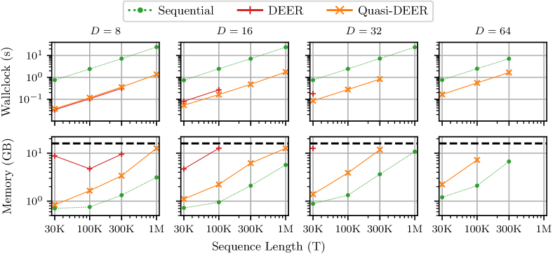
Figure 2: Evaluating an untrained GRU. Relative performance of sequential, DEER and quasi-DEER for evaluating a randomly initialized (and untrained) GRU on (Top Row) wall-clock time, averaged over 20 random seeds and (Bottom Row) memory, averaged over 3 random seeds. All experiments use a 16 GB V100 SMX2 (memory capacity indicated by the black dashed line) and Newton methods were run to convergence. Missing points in each series indicate the GPU ran out of memory. Quasi-DEER has a runtime commensurate with DEER, but with lower memory consumption, allowing quasi-DEER to work at scales where DEER cannot. The accuracy of the final converged solution is similar for all methods (see Figure 5 in Appendix B.1).

We show the results in Figure 2. Both DEER and quasi-DEER are as much as twenty times faster than sequential evaluation. We also see that quasi-DEER requires as much as an order of magnitude less memory than DEER, thus allowing the extension of the method into regimes previously infeasible for DEER. Note that the runtimes are similar between DEER and quasi-DEER for small networks, because although quasi-DEER steps are faster, DEER takes fewer iterations to converge. For larger networks, the difference in runtime is more pronounced. In Figure 6 of Appendix B.1.1 we show that in smaller $T$ and $D$ regimes we observe the expected sublinear time scaling with sequence length. This experiment confirms that quasi-DEER can replicate the performance of DEER, but with a smaller memory footprint.

6.2 Quasi-DEER for Training

We verify that quasi-DEER expedites training nonlinear RNN models. We replicate the third experiment from Lim et al. (2024), where a GRU is trained to classify C. elegans specimens from the time series of principal components of the worms’ body posture (Brown et al., 2013).

We show results in Figure 3. We see that the training dynamics under quasi-DEER leads to the similar validation accuracy trajectories, indicating there is no significant difference in training. However, every quasi-DEER training step is faster by a factor of $2.5$, despite performing $2$-$2.5$ times more Newton iterations per training step. This highlights how quasi-DEER can be used as a drop-in replacement for DEER when training nonlinear RNNs, bringing both time and memory savings.

DEER is prone to “spikes”, where orders of magnitude more steps are required for convergence (Figure 3, Middle Panel). While quasi-DEER is not as susceptible to these spikes (never more than half an order of magnitude), these instabilities motivate the study of stabilizing methods.

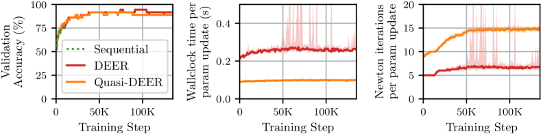
Figure 3: Training a GRU with DEER. Comparison of DEER and quasi-DEER during GRU training for the C. elegans time-series classification task (Section 6.2). Each time series has length $T=17,984$. We show the median, and 5-95% interval across a rolling window of 20 training steps. (Left) DEER and quasi-DEER have the similar validation accuracy trajectories, indicating similar training dynamics. The sequential trace shown is for 24 hours of training (compared to 11 and 4 for the whole DEER and quasi-DEER traces). (Center) Each quasi training iteration is 2.5 times faster than each DEER training iteration. Sequential training steps took more than 6 seconds each (not pictured). (Right) Each quasi training iteration requires (approximately) 2-2.5 times more Newton iterations to converge, indicating that each quasi Newton step is approximately 6 times faster than the corresponding DEER Newton step.

6.3 ELK and Quasi-ELK for Evaluating Autoregressive RNNs

We conclude by studying an application where these numerical instabilities in DEER are critical. We use a small autoregressive GRU (hidden dimension $N_{h}=3$), where the previous sampled value is input into the GRU at the next step. Such autoregressive architectures were not examined by Lim et al. (2024), but are an important class of models. We describe the precise details of the AR GRU we use in Appendix B.3. Crucially, the effective state used by all four methods must be expanded to include the current sampled output value, as well as the current GRU state.

Initialized AR GRU

We first repeat the analysis in Section 6.1 (and similar to the evaluation in Lim et al. (2024)) for evaluating a randomly initialized autoregressive GRU. We see in the top left panel of Figure 4 that all four parallelized methods converge rapidly and stably to the correct trace, indicated by a low mean absolute discrepancy (MAD) between the true trace and the generated trace.

Trained AR GRU

We then study a pre-trained GRU that generates a noisy sine wave (see Figure 4, Bottom Panel). The linear recurrence relation eq. 6 was numerically unstable in DEER and Quasi-DEER. To remedy these instabilities in DEER and quasi-DEER, we take the approach described earlier of setting the unstable parts of the trace to a fixed value (here zero). As described earlier, this reliably provides convergence; but at the cost of “resetting” the optimization for large swathes of the trace (Figure 4, Bottom Panel), slowing convergence (see Figure 4, Top Right Panel). This finding highlights how the instabilities of DEER — which are inherited from both pathologies of Newton’s method and the parallel recurrence — can be crippling in even very simple scenarios. While the resetting heuristic does facilitate convergence, the resulting convergence is drastically slower.

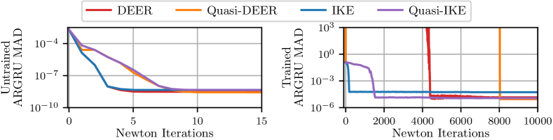
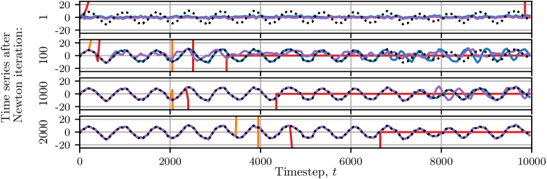
Figure 4: ELK stabilizes parallel evaluation of an AR GRU. (Top Left) The mean absolute difference (MAD) evaluated on the outputs converges rapidly for all four methods on a sequence generated by an untrained AR GRU. (Top Right) The MAD for evaluating a trained AR GRU. Undamped DEER variants are unstable and converge slowly. Damping via ELK stabilizes and accelerates convergence. (Bottom) The output after 1, 100, 1000, and 2000 Newton iterations. The black dotted line is the true trace. ELK and quasi-ELK converge rapidly, but DEER and quasi-DEER are unstable. The lines where DEER and quasi-DEER are zero show the heuristic of replacing NaN with zero.

We then apply ELK and quasi-ELK. We show the results in the top right and bottom panels of Figure 4. We select the trust region size with a one-dimensional search over log-spaced values between $10^{0}$ and $10^{7}$. We see ELK has stabilized convergence, with the evaluation never incurring numerical instabilities or requiring heuristics. Crucially, by taking more stable steps (and not needing stabilizing heuristics) ELK and quasi-ELK converge faster than DEER and quasi-DEER. ELK can stabilize and expedite the convergence of DEER, with quasi-ELK faster still (by wall-clock time).

However, on this task, all the parallelized methods (including DEER) have higher wall-clock time than sequential generation. Quasi-ELK is the fastest parallel method, taking 221 milliseconds for convergence, compared to sequential evaluation, taking 96 milliseconds. For comparison, DEER took 1,225 milliseconds. Quasi-ELK therefore still represents a large improvement in runtime over previous methods. We provide timing details and further discussion in Appendix B.3.2.

7 Conclusion

We proposed methods for scalable and stable parallel evaluation of nonlinear RNNs. DEER (Lim et al., 2024) achieves speedups over sequential evaluation, but incurs quadratic memory, cubic work, and can be numerically unstable. We therefore extended DEER to use quasi-Newton approximations, and provided a novel proof that both DEER and quasi-DEER converge globally. To stabilize DEER, we leveraged a connection between the Levenberg-Marquardt method and Kalman smoothing to enable parallel evaluation of RNNs, allowing us to stabilize DEER while still leveraging fast parallel filtering. We verified empirically that quasi-DEER, ELK, and quasi-ELK improve convergence across a range of metrics and examples. This result allows parallel evaluation of nonlinear RNNs to be scaled beyond what is possible with DEER. Our experiments also highlighted avenues for future research, such as leveraging structured approximations of the residual Jacobian, that still admit fast parallelism but are more accurate approximations, would allow for more accurate steps to be taken in quasi-DEER and quasi-ELK.

When selecting an approach, we offer the following advice: If rapid convergence is reliably observed, our experiments show that quasi-DEER provides the fastest convergence in terms of wall-clock time. If numerical stability is a concern, then ELK offers the most stable performance and convergence in the fewest Newton iterations, but quasi-ELK could be faster in wall-clock time and just as stable.

Acknowledgements

We thank John Duchi and the members of the Linderman Lab for helpful feedback. This work was supported by grants from the NIH BRAIN Initiative (U19NS113201, R01NS131987, & RF1MH133778), the NSF/NIH CRCNS Program (R01NS130789). X.G. would also like to acknowledge support from the Walter Byers Graduate Scholarship from the NCAA. S.W.L. is supported by fellowships from the Simons Collaboration on the Global Brain, the Alfred P. Sloan Foundation, and the McKnight Foundation. The authors have no competing interests to declare.

Appendix A Theoretical Results

A.1 Proof of Proposition 1

Proposition 1 If the Jacobians of the dynamics function $f$ are finite everywhere in the state space, then undamped Newton’s method will converge to the true solution, $\mathbf{s}^{*}$, of the fixed point eq. 2 in at most $T$ Newton iterations, for any initial $\mathbf{s}^{(0)}$.

Proof.

We prove this result by induction on the sequence length.

In general, the guess $\mathbf{s}^{(0)}$ need not equal the solution $\mathbf{s}^{*}$ anywhere. However, the initial state $\mathbf{s}_{0}$ and the dynamics functions $f$ are fixed. Therefore, $\mathbf{s}^{*}_{1}=f(\mathbf{s}_{0})$ and in general $\mathbf{s}^{*}_{t}=f(\mathbf{s}^{*}_{t-1})$. Thus, it follows from the initial condition of the DEER recurrence relation that $\mathbf{s}^{(i)}_{1}=\mathbf{s^{*}}_{1}$ for all $i\geq 1$.

Furthermore, we observe that if $\mathbf{s}_{t}^{(i)}=\mathbf{s}_{t}^{*}$ for all $t$ less than some $t^{(i)}$, then $\mathbf{r}_{t}(\mathbf{s}^{(i)})=\mathbf{0}$ for all $t<t^{(i)}$ by the definition of the residual in eq. 1. Therefore, as long as the Jacobians $\left\{\nicefrac{{\partial f}}{{\partial\mathbf{s}}}\right\}_{t=2}^{T}$ are finite, we see that the DEER linear recurrence relation necessarily gives $\Delta\mathbf{s}^{(i+1)}_{t}=\mathbf{0}$ for all $t<t^{(i)}$. Furthermore, because $\mathbf{s}_{t^{(i)}}^{*}=f(\mathbf{s}_{t}^{(i)})$, it follows that $\Delta\mathbf{s}_{t^{(i)}}^{(i+1)}=-\mathbf{r}_{t^{(i)}}(\mathbf{s}^{(i)})=\mathbf{s}^{*}_{t^{(i)}}-\mathbf{s}^{(i)}_{t^{(i)}}$. Thus, it follows that after applying another Newton iteration that $s_{t}^{(i+1)}=s_{t}^{*}$ for all $t<t^{(i)}+1$. The global convergence result and bound on Newton iterates now follows by induction. ∎

A.2 The Merit Function has no Local Minima

Proposition 3.

The merit function $\mathcal{L}(s)$ defined in (7) has a global minimum in the true trace $\mathbf{s}^{*}$, satisfying $\mathcal{L}(s^{*})=0$. It has no other local minima, i.e. no $\mathbf{s}$ such that $\nabla\mathcal{L}(\mathbf{s})=\mathbf{0}$ other than at the unique $\mathbf{s}^{*}$ for which $\mathbf{r}(\mathbf{s}^{*})=\mathbf{0}$.

Proof.

First, we observe that $\nabla\mathcal{L}(\mathbf{s})=J(\mathbf{s})^{T}\mathbf{r}(\mathbf{s})$, where $J(\mathbf{s})$ is defined as in (3). Because $J(\mathbf{s})$ is a lower triangular matrix with all entries on its diagonal equal to 1, it follows that all of its eigenvalues are equal to 1. Therefore, $J(\mathbf{s})$ is nonsingular for all $\mathbf{s}$. Thus, $J(\mathbf{s})$ has trivial nullspace for all $\mathbf{s}$, i.e. $J(\mathbf{s})^{T}\mathbf{r}(\mathbf{s})=\mathbf{0}\iff\mathbf{r}(\mathbf{s})=\mathbf{0}$. But only $\mathbf{s}^{*}$ satisfies $\mathbf{r}(\mathbf{s}^{*})=\mathbf{0}$. ∎

Appendix B Experimental Details

B.1 Quasi-DEER for Training

In this section we elaborate on our Experiment 1, discussed in Section 6.1. We hew closely to the experimental design of Section 4.1 of Lim et al. [2024], including 5 warm-up steps for all timing experiments. However, instead of running 5 seeds for 20 repetitions each, we run 20 seeds for 5 repetitions each, to get more converage over different evaluation (as the timing for each evaluation show low variance). We also include memory profiling experiments not present in Lim et al. [2024], which we discuss in more detail in Section B.1.3.

B.1.1 Numerical Precision of DEER and Quasi-DEER

In Figure 5 we qualitatively show that for the same example used in Figure 3 of Lim et al. [2024] that quasi-DEER converges within numerical precision to the correct trace in the untrained GRU benchmarking task discussed in Section 6.1. Similar results for DEER can be found in Section 4.1 of Lim et al. [2024].

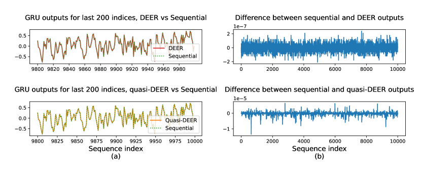
Figure 5: The accuracy of evaluating with parallelized methods (DEER and quasi-DEER) as opposed to sequential evaluation. The parallelized methods to the correct trace within numerical precision. The hidden state size is $D=4$ and the sequence length is $T=10,000$.

B.1.2 Different Scaling Regimes Depending on GPU Saturation

In Figure 6, we run the timing benchmarks of Section 6.1 on a wider range of sequence lengths $T$ and hidden state sizes $D$, on a large GPU (a V100 with 32 GB) and a smaller batch size (of 1). In doing so, we highlight that the parallel nature of DEER and quasi-DEER, as their wall-clock time scales sublinearly in the sequence length $T$ in smaller ($D$, $T$) regimes. However, we note that in the larger regimes considered in our main text and in Lim et al. [2024], we often observe linear scaling in the sequence length $T$ for the wall-clock time of DEER and quasi-DEER, even though these algorithms are still faster than sequential evaluation. Figure 6 shows good evidence that these parallel algorithms are suffering from saturation of the GPU, and would benefit from even more optimized parallel hardware.

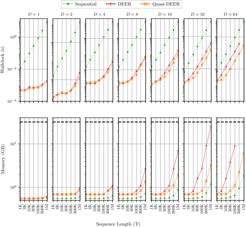
Figure 6: Evaluating an untrained GRU. Sublinear and linear timing regimes for parallelized algorithms. The above experiments were run on a 32 GB V100 with a batch size of 1. As in Figure 2, we use 20 seeds for timing, 3 sees for memory, and the dashed black line indicates the memory capacity of the GPU (32 GB). We observe that in smaller regimes in $D$ and $T$ that the wall-clock time shows sublinear scaling indicative of the use of parallel algorithms. However, when the GPU rank becomes saturated, the benefits of parallelization are reduced and we begin to see linear scaling in wall-clock time with $T$.

B.1.3 Memory Profiling Details

As we discussed in Section 4.1, quasi-DEER is $\mathcal{O}(TD)$ in memory while DEER is $\mathcal{O}(TD^{2})$ in memory because DEER uses dense Jacobians $\nicefrac{{\partial f}}{{\partial\mathbf{s}}}$ while quasi-DEER uses a diagonal approximation, $\mathrm{diag}(\nicefrac{{\partial f}}{{\partial\mathbf{s}}})$. However, to implement quasi-DEER with automatic differentiation, the most standard approach would be to compute the dense Jacobian, and then to take the diagonal; however, such an approach would still be $\mathcal{O}(TD^{2})$ in memory required. There are two implementation workarounds. One is to loop over computing partial derivatives, effectively trading time for memory. The second is simply derive the diagonal entries of the Jacobian for the architecture of interest. For the purpose of showcasing the $\mathcal{O}(TD)$ memory usage of quasi-DEER in Section 6.1, we take this second approach, deriving the diagonal entries of the Jacobian of the GRU nonlinear dynamics and implementing them in jax. However, for our other experiments, where memory capacity is not a problem, we simply use the less memory efficient version of quasi-DEER.

We also see linear memory scaling in evaluating the RNN sequentially. This behavior occurs because we JIT compile a lax.scan in JAX, and we track the maximum memory used on the GPU at any point in the computation. Because the inputs and the hidden states of the RNN scales are both of length $T$, the memory usage of $\mathcal{O}(T)$. While there may be more memory efficient ways to sequentially evaluate an RNN, we keep the same benchmarking structure as Lim et al. [2024] for to make comparison easier.

B.2 Quasi-DEER for Evaluation

Here we discuss the experimental details for the experiment in Section 6.2. We follow the same experimental set up as in Section 4.3 and Appendix B.3 of Lim et al. [2024]. As an aside, we note that the choice of hardware can impact behavior of the algorithms dramatically. For replicability, we run on the same hardware as Lim et al. [2024], using a 16GB V100 SXM2. However, we note that if we try to run these same experiments on A100, DEER struggles to converge numerically, although quasi-DEER shows no such difficulty. If we run on a CPU, both DEER and quasi-DEER converge numerically. On balance, on the eigenworms time series classification task, both DEER and quasi-DEER are numerically stable for the most part; the numerical instabilities we have observed for DEER on an A100 are likely specific to some particular detail of JAX/hardware interaction.

B.3 ELK and Quasi-ELK for Evaluating Autoregressive RNNs

Here we discuss our experimental details for our Experiment 3, discussed in Section 6.3.

B.3.1 AR GRU Architecture

The architecture is a GRU with hidden states $h_{t}\in\mathbb{R}^{3}$ and scalar inputs $x_{t}\in\mathbb{R}$. However, at any point in the sequence $t,$ we then readout the hidden state $h_{t}\in\mathbb{R}^{3}$ and use it to parameterize a mean $\mu_{t+1}\in\mathbb{R}$ and a quasi-variance $\sigma^{2}_{t+1}\in\mathbb{R}_{+}$. We then sample $x_{t+1}$ according to $x_{t+1}\sim\mathcal{N}(\mu_{t+1},\sigma_{t+1}^{2})$; this output $x_{t+1}$ is then fed into as the input to the AR GRU at time step $t+1$ to make the new hidden step $h_{t+1}$.

This AR GRU is trained using standard sequential evaluation and backpropagation-through-time to produce a noisy sine wave of length $10,\!000$. We train the AR GRU on $1024$ traces $x_{1:T}$ generated from a sine wave with amplitude 10 and white noise applied to each time step, and the training objective is to minimize the the negative log probability of the $x_{1:T}$.

Once the AR GRU has been trained, it can generate its own trace $\tilde{x}_{1:T}$ given an initial hidden state $h_{0}$ and noises $\epsilon_{1:T}$.

We note that such a system is Markovian with dimension $D=\dim(h)+\dim(x)$, as together the hidden state $h_{t}$ and output $x_{t+1}$ determine the next hidden state $h_{t+1}$ and output $x_{t+2}$. Thus, in the notation of Section 2, a hidden state $\mathbf{s}_{t}$ of the Markovian state space model is $\mathbf{s}_{t}=(x_{t+1},h_{t})$. Therefore, we can apply fixed point methods to try to find the correct trace $\mathbf{s}^{*}$ in a parallelized manner instead of autoregressively.

We note that one distinction of this set-up with respect to the notation developed in Section 2 is that the dynamics functions $f$ are effectively time-varying because the way in which $x_{t+2}$ is generated from $(x_{t+1},h_{t})$ depends on the noise $\epsilon_{t+2}$, the value of which varies across the sequence. However, all the results in the paper still apply after subsuming the input dependence into a time-varying dynamics function $f_{t}$.

B.3.2 Wall-clock Time Benchmark

The timing experiments were carried out as follows on an A100 GPU. We ran sequential evaluation of the trained AR GRU to produce noisy sine waves of length $T=10,\!000$, as well as the four parallelized method we consider in this paper (DEER, quasi-DEER, ELK, and quasi-ELK).

We ran 20 different random seeds (which lead to different values of the $\epsilon_{1:T}$ and therefore different nonlinear dynamics), and timed each for a total of 4 repetitions. Thus, for each of the five methods, we have a total of 80 timing runs. We record the wall-clock time needed to evaluate the length $T$ sequence sequentially, as well as wall-clock time, divided by $T$ needed to run $T$ Newton iterations of each of the parallelized methods (thus, we obtain the time per newton iteration for each of the parallelized methods).

Over these 80 timing runs, the sequential evaluation took an average of 96.2 milliseconds, with standard deviation of $1.55$ ms. We report the average time per newton iteration, the total number of newton iterations needed for convergence, and the total wall-clock time to convergence in Table 2. Note that the third column of Table 2 is the product of the first two columns.

We effectively read the number of Newton iteration to convergence off of the graphs in Figure 4, but find the number of Newton iterations to convergence to be quite stable across random seeds.

Table 2: Time to evaluate a length $T=10,000$ trained AR GRU using sequential vs parallelized methods. We note the dynamax package [Chang et al., 2023] we used for the parallel Kalman filter implementation in ELK is not optimized for speed, and hence these run times could be further improved.

Algorithm	Average time per Newton iteration $\pm$ std (ms)	Number of Newton iterations to convergence	Total time to convergence (ms)
Sequential Evaluation
Sequential	NA	NA	96.2
Parallelized Methods
DEER	$0.282\pm 0.0005$	4449	1255
quasi-DEER	$0.087\pm 0.0002$	7383	642
ELK	$3.600\pm 0.067$	172	619
quasi-ELK	$0.141\pm 0.0004$	1566	221

These timing results are illustrative of multiple themes of our paper. We see that while the undamped Newton steps are individually faster because they are carrying out fewer computations (they are just computing a linear recurrence relation, or equivalently an undamped Newton step, instead of computing a filtering pass, or equivalently solving a trust region problem). However, because the undamped Newton methods are numerically unstable, they take dramatically more Newton steps to convergence.

Similarly, we see that the quasi methods are dramatically faster than their dense counterparts as they are replace $\mathcal{O}(D^{3})$ matrix-matrix multiplication with $\mathcal{O}(D)$ diagonal matrix multiplication.

Thus, we find that our fastest parallelized method on wall-clock time is quasi-ELK, but even so it is approximately two times slower than sequentially evaluating this AR GRU. Therefore, an interesting direction for future work would be to characterize regimes where parallel methods can outperform sequential methods, and to investigate whether this autoregressive setting is such a regime, or whether parallelized methods can benefit from further speed-ups by leveraging adaptive trust region sizes, clever initialization strategies, or even more modern parallelized hardware.

References

- Bai et al. (2019) S. Bai, J. Z. Kolter, and V. Koltun. Deep equilibrium models. In Advances in Neural Information Processing Systems, volume 32, 2019.
- Bai et al. (2020) S. Bai, V. Koltun, and J. Z. Kolter. Multiscale deep equilibrium models. In Advances in Neural Information Processing Systems, volume 33, pages 5238–5250, 2020.
- Bai et al. (2021) S. Bai, V. Koltun, and J. Z. Kolter. Neural deep equilibrium solvers. In International Conference on Learning Representations, 2021.
- Beck et al. (2024) M. Beck, K. Pöppel, M. Spanring, A. Auer, O. Prudnikova, M. Kopp, G. Klambauer, J. Brandstetter, and S. Hochreiter. xlstm: Extended long short-term memory. arXiv preprint arXiv:2405.04517, 2024.
- Bell (1994) B. M. Bell. The iterated Kalman smoother as a Gauss–Newton method. SIAM Journal on Optimization, 4(3):626–636, 1994. doi: 10.1137/0804035.
- Bell and Cathey (1993) S. M. Bell and F. W. Cathey. The iterated Kalman filter update as a Gauss-Newton method. IEEE Transactions on Automatic Control, 38(2):294–297, 1993.
- Blelloch (1990) G. E. Blelloch. Prefix sums and their applications. Technical Report CMU-CS-90-190, Carnegie Mellon University, School of Computer Science, 1990.
- Brown et al. (2013) A. E. Brown, E. I. Yemini, L. J. Grundy, T. Jucikas, and W. R. Schafer. A dictionary of behavioral motifs reveals clusters of genes affecting caenorhabditis elegans locomotion. Proceedings of the National Academy of Sciences, 110(2):791–796, 2013.
- Broyden (1970) C. Broyden. The convergence of a class of double-rank minimization algorithms. IMA Journal of Applied Mathematics, 6(1):76–90, 1970.
- Chang et al. (2023) P. Chang, G. Harper-Donnelly, A. Kara, X. Li, S. Linderman, and K. Murphy. Dynamax: State space models library in jax, 2023. URL https://github.com/probml/dynamax.
- Chen et al. (2018) R. T. Q. Chen, Y. Rubanova, J. Bettencourt, and D. Duvenaud. Neural ordinary differential equations. In Advances in Neural Information Processing Systems, volume 31, pages 6571–6583, 2018.
- Chen and Oliver (2013) Y. Chen and D. S. Oliver. Levenberg–Marquardt forms of the iterative ensemble smoother for efficient history matching and uncertainty quantification. Computational Geosciences, 17(4):689–703, 2013. doi: 10.1007/s10596-013-9351-5.
- Cho et al. (2014) K. Cho, B. van Merriënboer, Ç. Gülçehre, D. Bahdanau, F. Bougares, H. Schwenk, and Y. Bengio. Learning phrase representations using RNN encoder-decoder for statistical machine translation. arXiv preprint arXiv:1406.1078, 2014.
- Conn et al. (2000) A. Conn, N. Gould, and P. Toint. Trust Region Methods, volume 1. Society for Industrial and Applied Mathematics, 2000.
- Doikov and Nesterov (2023) N. Doikov and Y. Nesterov. Gradient regularization of Newton method with Bregman distances. Mathematical Programming, pages 1–25, 2023.
- Fletcher (1970) R. Fletcher. A new approach to variable metric algorithms. The Computer Journal, 13(3):317–322, 1970.
- Fu et al. (2024) Y. Fu, P. Bailis, I. Stoica, and H. Zhang. Break the sequential dependency of LLM inference using lookahead decoding. arXiv preprint arXiv:2402.02057, 2024.
- Goldfarb (1970) D. Goldfarb. A family of variable-metric methods derived by variational means. Mathematics of Computation, 24(109):23–26, 1970.
- Goodfellow et al. (2016) I. Goodfellow, Y. Bengio, and A. Courville. Deep Learning. MIT Press, 2016. ISBN 978-0262035613.
- Gu and Dao (2023) A. Gu and T. Dao. Mamba: Linear-time sequence modeling with selective state spaces. arXiv preprint arXiv:2312.00752, 2023.
- Gu et al. (2021) A. Gu, K. Goel, and C. Ré. Efficiently modeling long sequences with structured state spaces. In International Conference on Learning Representations (ICLR), 2021.
- Hochreiter and Schmidhuber (1997) S. Hochreiter and J. Schmidhuber. Long short-term memory. Neural computation, 9(8):1735–1780, 1997.
- Hooker (2021) S. Hooker. The hardware lottery. Communications of the ACM, 64(12):58–65, 2021.
- Katharopoulos et al. (2020) A. Katharopoulos, A. Vyas, N. Pappas, and F. Fleuret. Transformers are RNNs: Fast autoregressive transformers with linear attention. In International Conference on Machine Learning, pages 5156–5165. PMLR, 2020.
- Kidger (2021) P. Kidger. On Neural Differential Equations. PhD thesis, University of Oxford, 2021.
- Kolter et al. (2020) Z. Kolter, D. Duvenaud, and M. Johnson. Deep implicit layers - neural odes, deep equilibrium models, and beyond, 2020. NeurIPS 2020 Tutorial.
- Levenberg (1944) K. Levenberg. A method for the solution of certain non-linear problems in least squares. Quarterly of Applied Mathematics, 2:164–168, 1944.
- Lim et al. (2024) Y. H. Lim, Q. Zhu, J. Selfridge, and M. F. Kasim. Parallelizing non-linear sequential models over the sequence length. In International Conference on Learning Representations, 2024.
- Liu and Nocedal (1989) D. C. Liu and J. Nocedal. On the limited memory BFGS method for large scale optimization. Mathematical Programming, 45(1-3):503–528, 1989.
- Mandel et al. (2016) J. Mandel, E. Bergou, S. Gürol, S. Gratton, and I. Kasanickỳ. Hybrid Levenberg–Marquardt and weak-constraint ensemble Kalman smoother method. Nonlinear Processes in Geophysics, 23(2):59–73, 2016.
- Marquardt (1963) D. W. Marquardt. An algorithm for least-squares estimation of nonlinear parameters. Journal of the Society for Industrial and Applied Mathematics, 11(2):431–441, 1963.
- Martens and Grosse (2015) J. Martens and R. Grosse. Optimizing neural networks with Kronecker-factored approximate curvature. In International conference on machine learning, pages 2408–2417. PMLR, 2015.
- Martin and Cundy (2018) E. Martin and C. Cundy. Parallelizing linear recurrent neural nets over sequence length. In International Conference on Learning Representations, 2018.
- Massaroli et al. (2021) S. Massaroli, M. Poli, S. Sonoda, T. Suzuki, J. Park, A. Yamashita, and H. Asama. Differentiable multiple shooting layers. Advances in Neural Information Processing Systems, 34:16532–16544, 2021.
- Merrill et al. (2024) W. Merrill, J. Petty, and A. Sabharwal. The illusion of state in state-space models. arXiv preprint arXiv:2404.08819, 2024.
- Mihaylova and Martins (2019) T. Mihaylova and A. F. T. Martins. Scheduled sampling for transformers. In F. Alva-Manchego, E. Choi, and D. Khashabi, editors, Proceedings of the 57th Annual Meeting of the Association for Computational Linguistics: Student Research Workshop, pages 351–356, Florence, Italy, July 2019. Association for Computational Linguistics. doi: 10.18653/v1/P19-2049.
- Nesterov and Polyak (2006) Y. Nesterov and B. T. Polyak. Cubic regularization of newton method and its global performance. Mathematical Programming, 108(1):177–205, 2006.
- Nocedal and Wright (2006) J. Nocedal and S. J. Wright. Numerical Optimization. Springer, 2 edition, 2006.
- Oord et al. (2016) A. v. d. Oord, S. Dieleman, H. Zen, K. Simonyan, O. Vinyals, A. Graves, N. Kalchbrenner, A. Senior, and K. Kavukcuoglu. Wavenet: A generative model for raw audio. arXiv preprint arXiv:1609.03499, 2016.
- Ortega and Rheinboldt (2000) J. M. Ortega and W. C. Rheinboldt. Iterative Solution of Nonlinear Equations in Several Variables. SIAM, 2000.
- Orvieto et al. (2023) A. Orvieto, S. L. Smith, A. Gu, A. Fernando, C. Gulcehre, R. Pascanu, and S. De. Resurrecting recurrent neural networks for long sequences. In International Conference on Machine Learning, pages 26670–26698. PMLR, 2023.
- Parnichkun et al. (2024) R. N. Parnichkun, S. Massaroli, A. Moro, J. T. Smith, R. Hasani, M. Lechner, Q. An, C. Ré, H. Asama, S. Ermon, T. Suzuki, A. Yamashita, and M. Poli. State-free inference of state-space models: The transfer function approach. arXiv preprint arXiv:2405.06147, 2024.
- Poli et al. (2023) M. Poli, S. Massaroli, E. Nguyen, D. Y. Fu, T. Dao, S. Baccus, Y. Bengio, S. Ermon, and C. Ré. Hyena hierarchy: Towards larger convolutional language models. In International Conference on Machine Learning, pages 28043–28078. PMLR, 2023.
- Romero et al. (2021) D. W. Romero, A. Kuzina, E. J. Bekkers, J. M. Tomczak, and M. Hoogendoorn. Ckconv: Continuous kernel convolution for sequential data. arXiv preprint arXiv:2102.02611, 2021.
- Santilli et al. (2023) A. Santilli, S. Severino, E. Postolache, V. Maiorca, M. Mancusi, R. Marin, and E. Rodolà. Accelerating transformer inference for translation via parallel decoding. In Proceedings of the 61st Annual Meeting of the Association for Computational Linguistics (Volume 1: Long Papers), pages 12336–12355, Toronto, Canada, July 2023. Association for Computational Linguistics. doi: 10.18653/v1/2023.acl-long.689.
- Särkkä and García-Fernández (2021) S. Särkkä and Á. F. García-Fernández. Temporal parallelization of bayesian smoothers. IEEE Transactions on Automatic Control, 66(1):299–306, 2021. doi: 10.1109/TAC.2020.2976316.
- Shanno (1970) D. Shanno. Conditioning of quasi-newton methods for function minimization. Mathematics of Computation, 24(111):647–656, 1970.
- Smith et al. (2021) J. Smith, S. Linderman, and D. Sussillo. Reverse engineering recurrent neural networks with Jacobian switching linear dynamical systems. Advances in Neural Information Processing Systems, 34:16700–16713, 2021.
- Smith et al. (2023) J. T. Smith, A. Warrington, and S. W. Linderman. Simplified state space layers for sequence modeling. In International Conference on Learning Representations (ICLR), 2023.
- Sorenson (1966) H. W. Sorenson. Kalman filtering techniques. In H. W. Sorenson, editor, Kalman Filtering: Theory and Application, page 90. IEEE Press, New York, 1966.
- Steihaug (1983) T. Steihaug. The conjugate gradient method and trust regions in large scale optimization. SIAM Journal on Numerical Analysis, 20(3):626–637, 1983.
- Sussillo and Barak (2013) D. Sussillo and O. Barak. Opening the black box: Low-dimensional dynamics in high-dimensional recurrent neural networks. Neural Computation, 25(3):626–649, 2013.
- Särkkä (2013) S. Särkkä. Bayesian Filtering and Smoothing. Cambridge University Press, Cambridge, UK, 2013. ISBN 978-1-107-03385-3.
- Särkkä and Svensson (2020) S. Särkkä and L. Svensson. Levenberg-Marquardt and line-search extended Kalman smoothers. In ICASSP 2020 - 2020 IEEE International Conference on Acoustics, Speech and Signal Processing (ICASSP), pages 5875–5879. IEEE, 2020. doi: 10.1109/ICASSP40776.2020.9054764.
- Vaswani et al. (2017) A. Vaswani, N. Shazeer, N. Parmar, J. Uszkoreit, L. Jones, A. N. Gomez, Ł. Kaiser, and I. Polosukhin. Attention is all you need. In Proceedings of the 31st International Conference on Neural Information Processing Systems, pages 6000–6010, 2017.