OFDM-Based Positioning with Unknown Data Payloads: Bounds and Applications to LEO PNT

Abstract

This paper presents bounds, estimators, and signal design strategies for exploiting both known pilot resources and unknown data payload resources in toa-based positioning systems with ofdm signals. It is the first to derive the zzb on toa estimation for ofdm signals containing both known pilot and unknown data resources. In comparison to the crlb derived in prior work, this zzb captures the low-snr thresholding effects in toa estimation and accounts for an unknown carrier phase. The derived zzb is evaluated against crlb and empirical toa error variances. It is then evaluated on signals with resource allocations optimized for pilot-only toa estimation, quantifying the performance gain over the best-case pilot-only signal designs. Finally, the positioning accuracy of maximum-likelihood and decision-directed estimators is evaluated on simulated leo ntn channels and compared against their respective zzb.

I Introduction

Positioning services within existing wireless communications networks are becoming an increasingly important source of accurate localization. Such services can provide exceptional accuracy due to their access to large bandwidths and widespread deployment, making them an attractive alternative to traditional gnss positioning. leo ntn in particular are a prime candidate for accurate user positioning services because of their ability to provide near-global coverage and strong signals with exceptionally large bandwidths [1, 2]. These leo ntn are undergoing a massive expansion in satellite deployment [3], further increasing their viability as the new standard for global positioning while simultaneously providing high-throughput communications.

An overwhelming majority of communications networks, including the 5G ntn standard [3], operate through ofdm, which divides the spectrum into time and frequency resource elements that may be allocated with either known pilot resources or unknown data resources. Since the structure of these pilot resources is known to users in the network, users may obtain toa estimates by correlating their received signal against the known pilot resources. These toa estimates may then be used in positioning protocols such as pseudorange multilateration, tdoa, or rtt [4]. But this scheme creates a challenging design tradeoff: allocating additional pilot resources improves positioning accuracy at the expense of data throughput, since ofdm resources must be diverted from data [5]. This tradeoff becomes especially complex for satellites in ntn, which must additionally manage their power consumption when balancing the tradeoff between communications and positioning services [2]. Such a “zero-sum game” poses problems for rapidly expanding ntn tasked with handling an ever-growing demand for both increased positioning accuracy and higher data rates. However, a new and enticing scheme emerges if users exploit both pilot resources and data resources in their toa estimation.

Two approaches exist for users to exploit data resources in their toa estimation: dd and ml estimation. The decision-directed estimator makes hard decoding decisions on the unknown data and then correlates the received signal against both the pilot resources and decoded data to improve estimation accuracy. While dd estimators are efficient and effective at high snr, they are prone to decoding errors. Although these decoding errors may be mitigated through error correcting codes, such codes may not be usable for data resources intended for other users since networks may intentionally obfuscate the coding from other users; witness the scrambling by the rnti in lte and 5G nr. In contrast to dd estimators, ml estimators, commonly referred to as nda estimators in prior work when no known pilots are used [6, 7], do not make hard decoding decisions but instead evaluate the likelihood of data resources over all symbols in the constellation. Since an overwhelming majority of the spectrum in communications networks is allocated to data resources, these dd and ml estimators can harness a much greater amount of signal power compared to the pilot-only estimator, resulting in significantly reduced toa estimation errors.

When evaluating signals for toa estimation, it is crucial to consider the impact that resource allocation has on the toa likelihood function, which exhibits a mainlobe centered around the true toa, sidelobes located away from the true toa outside the mainlobe, and grating lobes caused by aliasing. At high snr, toa estimation errors will be concentrated near the true toa within the mainlobe. At low snr, however, toa estimates may latch on to sidelobes, significantly increasing estimation error variance [8, 9, 10]. Bounds such as the Barankin bound [11, 12] and zzb [13] were derived to capture the behavior of this thresholding effect, which is ignored by the simpler crlb. When only pilot resources are used in toa estimation, the likelihood function is closely related to the acf. However, the inclusion of unknown data resources in the likelihood function alters its shape in a complex manner, potentially introducing new sidelobes and sharpening the mainlobe. A bound that captures both the effects of unknown data and low snr is needed to accurately characterize the positioning performance of dd and ml estimators.

leo ntn are especially amenable to positioning with unknown data resources. The large satellite constellation sizes increase the likelihood of a los path between users and satellites. Furthermore, phased arrays at both ends provide exceptional multipath mitigation. Finally, leo satellites may be able to pre-compensate for Doppler due to their highly directive beams and small cell size. As a result, the fading in the post-beamforming channels remains exceptionally flat across wide bandwidths — as large as $240\text{\,}\mathrm{MHz}$ in the case of Starlink [14]. Under these favorable channels conditions, users only need to estimate and compensate for the toa and carrier phase to equalize the received signal and begin decoding data.

This paper derives the zzb on toa estimation error variance for ofdm signals containing both pilot resources and unknown data resources. The derived zzb is then compared against crlb derived in prior work and against empirical toa estimation error variance. Empirical toa estimates are obtained with both ml and dd estimators. Three variants of ml estimators are considered: one that exploits only pilot resources, another based on only data resources, and a third that harnesses both pilot and data resources. These will be referred to as the pilot-only, data-only, and pilot-plus-data ml estimators, respectively. Candidate resource allocations are then generated over a range of snr that optimize the placement of prs in the frequency domain to minimize the pilot-only toa zzb. The pilot-plus-data toa zzb is then evaluated on these optimized signals to quantify the reduction in toa estimation error that can be achieved over the optimal allocations for pilot-only estimation. Finally, leo ntn channels are simulated for a satellite constellation servicing a single cell. The positioning accuracy of a user in the serviced cell is evaluated using Monte Carlo methods for the pilot-only ml, data-only ml, pilot-plus-data ml, and dd estimators. These results are then compared against the derived zzb.

I-A Prior Work

Prior work has studied several toa-based positioning algorithms with ofdm signals. Algorithms such as tdoa, pseudorange multilateration, and rtt are supported within the existing 5G nr standards [4]. More advanced approaches have demonstrated accurate positioning with 5G nr signals using both toa and aoa measurements in an ekf [15] and using multipath parameter estimates obtained from signals with optimized beam power allocations [16]. Alternatively, lte [17] and 5G nr [18, 19] signals have been used as sop for positioning, a paradigm that requires no cooperation between the user and the network. While exceptional positioning accuracy is demonstrated in this prior work, both the network-supported and sop methods only obtain position estimates from known reference signals embedded in the ofdm signal and do not exploit the vast quantity of unknown data resources that are present in typical lte and 5G nr downlink signals. The presence of ofdm reference signals has also been detected in a cognitive manner for sop positioning [19, 20], but this approach still relies on the allocation of reference signals by the network.

The analysis of positioning within communications networks has been extended to the context of leo ntn. Scheduling for leo constellations providing both communications and positioning services has been analyzed in [2]. The authors in [21] optimized leo beamforming and beam scheduling to minimize the user positioning crlb. This work demonstrates the potential improvements leo positioning services may provide over existing gnss solutions. However, prior work has not yet analyzed ofdm resource allocation for leo positioning nor explored the potential for exploiting data resources in toa estimation.

Outside of positioning, dd and nda estimation have been thoroughly studied in the context of communications. Prior work has analyzed dd estimators for ofdm frequency-offset estimation [22], ofdm channel estimation in high-velocity channels [23], and mimo channel tracking [24]. The authors in [25] propose a dd channel estimator for overcoming pilot contamination in cell-free massive mimo networks. This body of work demonstrates the potential improvements in estimator accuracy that may be gained through hard decoding decisions on unknown data. Similarly, prior work has analyzed nda estimators for ofdm frequency-offset estimation [26], ofdm timing recovery [27], and ofdm snr estimation [28]. Prior work has also studied the crlb of nda estimation. Bellili et al. derived a crlb for nda time [29] and frequency [6] estimation for square-QAM constellations that is tighter than the simpler mcrlb. The authors in [30] also propose a nda toa estimator that uses importance sampling to reduce computational costs, and they compare its performance against the mcrlb.

Whereas prior work has extensively studied nda and dd estimators for communications purposes, only a limited body of work has studied their applicability to positioning. The authors in [31] proposed a nda aoa estimator for positioning with Gaussian frequency-shift-keying signals. Wang et al. proposed a semiblind ofdm range tracker which, after initialization with known pilot resources, tracks the multipath components of the channel using dd decoding decisions and a Kalman filter [32]. Similarly, the authors in [33] proposed a semiblind channel estimator for positioning that improves its estimates of the multipath components of the channel using dd decoding, comparing performance against the mcrlb. Mensing et al. proposed a dd toa estimator for tdoa positioning with intercell interference [34]. This work demonstrates how unknown data payloads can be exploited, either through nda or dd estimation, to improve positioning accuracy within communications networks. However, these papers do not compare nda and dd estimators against one another to understand how each estimator’s errors change with snr. Furthermore, [31] and [33] did not consider ofdm signals, and [31] did not consider toa-based positioning. Finally, [31, 33, 34] compared estimator accuracy only against the crlb, which is unable to capture low-snr thresholding effects.

To overcome the limitations of the crlb, several studies have used the zzb for analyzing positioning performance in ofdm systems with pilot-only toa estimation. Prior work has used the zzb to characterize the toa precision of different parameterizations of ofdm pilot resource allocations [5, 35, 36, 37]. Furthermore, the zzb has been used as an optimization criteria to solve for ofdm pilot resource allocations that minimize toa estimation errors [38]. The zzb on direct position estimation has also been derived in [39]. However, prior work has not derived the zzb in the context of unknown data or for nda estimation.

I-B Contributions

The main contributions of this paper are as follows:

• A novel derivation of the zzb on toa estimation error variance for ofdm signals with unknown data resources. This novel bound is compared against the crlb, mcrlb, and empirical errors from Monte-Carlo simulation.

• A comparison of the pilot-only and pilot-plus-data zzb for ofdm signals with resources optimized for pilot-only toa estimation. This comparison provides insights into the potential gains achieved by exploiting unknown data and informs how pilot resources can be allocated to minimize overhead while meeting toa accuracy requirements.

• Evaluation of the empirical positioning errors achieved by both ml and dd estimators on simulated leo satellite channels in comparison to the zzb.

The remainder of this paper is organized as follows. Section II introduces the signal model. Section III defines the toa crlb and derives the toa zzb for ofdm signals with payloads containing unknown data. Section IV defines the ml estimators for the pilot-only, data-only, and pilot-plus-data cases as well as the dd estimator. Section V-A compares the derived zzb against the crlb and Monte Carlo toa errors. Section V-B evaluates the pilot-plus-data zzb on signals with resource allocations optimized for pilot-only estimation. Section V-C evaluates the positioning accuracy of the pilot-only ml, data-only ml, pilot-plus-data ml, and dd estimators on simulated leo ntn channels, comparing them against the derived zzb. Finally, Section VI closes the paper by drawing conclusions from the results.

Notation: Column vectors are denoted with lowercase bold, e.g., $\bm{x}$. Matrices are denoted with uppercase bold, e.g., $\bm{X}$. Scalars are denoted without bold, e.g., $x$. The $i$th entry of a vector $\bm{x}$ is denoted $x[i]$ or in shorthand as $x_{i}$. The Euclidean norm is denoted $||\bm{x}||$. The cardinality of a set $\mathcal{S}$ is denoted $|\mathcal{S}|$. Real transpose is represented by the superscript $T$ and conjugate transpose by the superscript $H$. The Q-function is denoted as $Q(\cdot)$. Zero-based indexing is used throughout the paper; e.g., $x[0]$ refers to the first element of $\bm{x}$.

II Signal Model

Consider an ofdm signal with $K$ subcarriers, $N_{\text{sym}}$ symbols, a subcarrier spacing of $\Delta_{\text{f}}\;$\text{\,}\mathrm{Hz}$$, and a payload $x_{m}[k]$ for symbol indices $m\in\mathcal{M}$ and subcarrier indices $k\in\mathcal{K}$, where $\mathcal{M}=\{0,1,\ldots,N_{\text{sym}}-1\}$ and $\mathcal{K}=\{0,1,\ldots,K-1\}$. Let $d[k]$ be the mapping from subcarrier indices to offsets in frequency from the carrier in units of subcarriers. This map is defined as $d[k]=k$ for $k=0,1,\ldots,\textstyle\frac{K}{2}-1$ and $d[k]=k-K$ for $k=\textstyle\frac{K}{2},\textstyle\frac{K}{2}+1,\ldots,K-1$. This signal propagates through a doubly-selective channel at a carrier frequency $f_{\text{c}}$ with baseband frequency-domain channel coefficients $h_{m}[k]$ and experiences a los time delay $\tau$, phase shift $\phi$, and awgn $v_{m}[k]\sim\mathcal{CN}(0,\sigma^{2})$. Assuming negligible ici due to small Doppler and negligible isi due to a sufficiently long cyclic-prefix, the baseband received signal $y_{m}[k]$ is modeled in the frequency domain as

$$y_{m}[k] =\alpha_{m}[k]x_{m}[k]+v_{m}[k],$$ (1)

$$\alpha_{m}[k] =h_{m}[k]\exp\left(-j2\pi d[k]\Delta_{\text{f}}\tau+j\phi\right).$$ (2)

If the channel coefficients are constant across frequency and time, the complex gain $\alpha_{m}[k]$ can be instead modeled as

$$\alpha_{m}[k] =\sqrt{g}\exp\left(-j2\pi d[k]\Delta_{\text{f}}\tau+j\phi\right),$$ (3)

where $g$ is the channel gain. The bounds and estimators of this paper are derived under the frequency-flat time-invariant model in (3), while the simulated channels in the results use the frequency-selective time-varying model in (2).

The payload $x_{m}[k]$ may contain either pilot resources, data resources, or be empty. Define $\mathcal{K}_{m}^{\text{P}}$ as the set of subcarrier indices containing pilot resources, $\mathcal{K}_{m}^{\text{D}}$ as the set of subcarrier indices containing data resources, and $\tilde{\mathcal{K}}_{m}\triangleq\mathcal{K}_{m}^{\text{P}}\bigcup\mathcal{K}_{m}^{\text{D}}$ as their union, during symbol $m$. Each data resource is modeled as randomly selected from a symbol constellation $\mathcal{C}$ with uniform probability and statistical independence from all other resource elements. This is expressed as $x_{m}[k]=c_{m}[k]$ and $P(c_{m}[k]=c_{\text{sym}})=\frac{1}{|\mathcal{C}|}$ for $m\in\mathcal{M}$, $k\in\mathcal{K}_{m}^{\text{D}}$, and $c_{\text{sym}}\in\mathcal{C}$. Furthermore, the constellation is modeled as having unit average power such that $\mathbb{E}\left[|x_{m}[k]|^{2}\right]=1$.

III TOA Estimation Error Bounds

Let $\hat{\tau}$ be an unbiased estimate of the true toa $\tau$ and define $\gamma_{m}[k]=\textstyle\frac{|\alpha_{m}[k]|^{2}}{\sigma^{2}}$ as the snr at subcarrier $k$ during symbol $m$. This section will define bounds on the toa estimation error variance $\mathbb{E}\left[(\hat{\tau}-\tau)^{2}\right]$ under the simplified signal model in (3).

III-A Cramer-Rao Bounds

The simplest bound is the crlb when $\hat{\tau}$ is estimated using only pilot resources, which takes the form [40]

$$\mathbb{E}\left[(\hat{\tau}-\tau)^{2}\right] \geq\sigma_{\text{CRLB,P}}^{2}=I_{\text{CRLB,P}}^{-1}$$ (4)

$$I_{\text{CRLB,P}} \triangleq 8\pi^{2}\Delta_{\text{f}}^{2}\sum_{m\in\mathcal{M}}\sum_{k\in\mathcal{K}_{m}^{\text{P}}}d^{2}[k]\gamma_{m}[k].$$ (5)

In comparison to the pilot-only crlb, the derivation of the crlb for the data-only estimator is more difficult since the likelihood function for each resource element is a Gaussian mixture distribution function with each Gaussian centered at each symbol in the constellation $\mathcal{C}$. One simplifying approach is to derive the mcrlb [41] by conditioning on the unknown symbols. This simplifies to a form similar to the pilot-only crlb

$$\mathbb{E}\left[(\hat{\tau}-\tau)^{2}\right] \geq\sigma_{\text{MCRLB}}^{2}=I_{\text{MCRLB}}^{-1}$$ (6)

$$I_{\text{MCRLB}} \triangleq 8\pi^{2}\Delta_{\text{f}}^{2}\sum_{m\in\mathcal{M}}\sum_{k\in\mathcal{K}_{m}^{\text{D}}}d^{2}[k]\gamma_{m}[k].$$ (7)

A tighter crlb for unknown data is derived in [6] without using the mcrlb. While this bound was derived for frequency estimation, it is easily mapped to toa estimation with ofdm signals. This crlb takes the form

$$\mathbb{E}\left[(\hat{\tau}-\tau)^{2}\right]\geq\sigma_{\text{CRLB,D}}^{2}=I_{\text{CRLB,D}}^{-1},$$ (8)

where

$$I_{\text{CRLB,D}}\triangleq 8\pi^{2}\Delta_{\text{f}}^{2}\sum_{\begin{subarray}{c}m\in\mathcal{M}\\ k\in\mathcal{K}_{m}^{\text{D}}\end{subarray}} \left(\frac{1+\gamma_{m}[k]}{A_{2}}\psi(\gamma_{m}[k])-\gamma_{m}[k]\right)$$

$$\times d^{2}[k]\gamma_{m}[k],$$ (9)

and $\psi(\cdot)$ and $A_{2}$ are defined in [6, Eqs. (37)-(38)].

These crlb are useful for analyzing the high-snr precision of toa estimators, and the crlb from [6] importantly captures the increased errors caused by uncertainty in the symbol selected from the constellation, making the bound in (9) tighter than the mcrlb in (7). These fundamental error bounds can provide valuable insights into the efficiency of estimators and can serve as an optimization criteria for evaluating different signal designs and resource allocations. However, the crlb ignore the impact that sidelobes in the likelihood function have on estimation error, making these bounds inapt at lower snr [5].

III-B Ziv-Zakai Bounds

The zzb is superior to the crlb for toa estimation analysis because it captures the low-snr thresholding effects caused by sidelobes. The bound considers a binary detection problem with equally-likely hypotheses: (1) the received signal experienced delay $\tau_{0}$ and phase $\phi_{0}$, and (2) the received signal experienced delay $\tau_{0}+\tau_{1}$ and phase $\phi_{0}+\phi_{1}\pmod{2\pi}$. Define $\bm{\theta}\triangleq[\tau,\;\phi]^{T}$, $\bm{\theta}_{0}\triangleq[\tau_{0},\;\phi_{0}]^{T}$, and $\bm{\theta}_{1}\triangleq[\tau_{0}{+}\tau_{1},\;\phi_{0}{+}\phi_{1}\pmod{2\pi}]^{T}$. $\bm{\theta}$ is treated as a random variable with a known a priori distribution. The hypothesis test can be expressed as

$$\frac{p(\bm{y}|\bm{\theta}{=}\bm{\theta}_{0})}{p(\bm{y}|\bm{\theta}{=}\bm{\theta}_{1})}\underset{\mathcal{H}_{1}}{\overset{\mathcal{H}_{0}}{\gtrless}}\nu,\quad\quad\genfrac{}{}{0.0pt}{}{\mathcal{H}_{0}\;:\;\bm{\theta}=\bm{\theta}_{0}}{\mathcal{H}_{1}\;:\;\bm{\theta}=\bm{\theta}_{1}},$$ (10)

where $\bm{y}$ is the vector containing all $y_{m}[k]$ for $m\in\mathcal{M}$ and $k\in\tilde{\mathcal{K}}_{m}$, and $\nu$ is the detection threshold. The zzb is concerned with the minimum error probability of this hypothesis test, which corresponds to a threshold of $\nu=1$ when $\mathcal{H}_{0}$ and $\mathcal{H}_{1}$ are assumed equally-likely.

As in [38], the time delays will be normalized by the ofdm sampling period $T_{\text{s}}=\textstyle\frac{1}{K\Delta_{\text{f}}}$, creating $z\triangleq\textstyle\frac{\tau}{T_{\text{s}}}$, $z_{0}\triangleq\textstyle\frac{\tau_{0}}{T_{\text{s}}}$ and $z_{1}\triangleq\textstyle\frac{\tau_{1}}{T_{\text{s}}}$. The minimum error probability of this detection problem is assumed to be shift-invariant, allowing the hypotheses to be simplified without loss of generality by assuming $\tau_{0}=0$ and $\phi_{0}=0$. Then the log of the likelihood ratio in (10) can be denoted

$$\log\Lambda(\bm{y},\bm{\theta}_{1})\triangleq\log{p(\bm{y}|\bm{\theta}{=}\bm{\theta}_{0})}-\log{p(\bm{y}|\bm{\theta}{=}\bm{\theta}_{1})},$$ (11)

and the minimum error probability of the hypothesis test is defined as the probability that the log-likelihood ratio in (11), conditioned on $\bm{\theta}=\bm{\theta}_{0}$, is less than zero:

$$P_{\text{min}}(z_{1},\phi_{1})\triangleq P\left(\log\Lambda(\bm{y},\bm{\theta}_{1})<0\right|\bm{\theta}{=}\bm{\theta}_{0}).$$ (12)

Define $\bm{R}_{\bm{\theta}}$ as the estimation error covariance of $\bm{\theta}$ and $\mathcal{V}\{\cdot\}$ as the valley-filling function [42]. Assuming a priori knowledge that the toa is uniformly distributed on $[0,T_{\text{a}}]$ and the phase is uniformly distributed on $[0,2\pi]$, and noting the scale-invariance of the valley-filling function, the zzb on toa error variance can be defined as [43]

$$\mathbb{E}\left[(\hat{\tau}-\tau)^{2}\right]=\bm{a}^{T}\bm{R}_{\bm{\theta}}\bm{a}$$ (13)

$$\geq\sigma_{\text{ZZB}}^{2}$$

$$\triangleq\frac{1}{T_{\text{a}}}\int_{0}^{T_{\text{a}}}\tau_{1}\mathcal{V}\{(T_{\text{a}}-\tau_{1})\max_{\phi_{1}}\left[P_{\text{min}}(\tau_{1}/T_{s},\phi_{1})\right]\}d\tau_{1}$$

$$=\frac{T_{\text{s}}^{2}}{N_{\text{a}}}\int_{0}^{N_{\text{a}}}z_{1}\mathcal{V}\{(N_{\text{a}}-z_{1})\max_{\phi_{1}}\left[P_{\text{min}}(z_{1},\phi_{1})\right]\}dz_{1},$$

where $N_{\text{a}}\triangleq\textstyle\frac{T_{\text{a}}}{T_{\text{s}}}$.

Expressions for $P_{\text{min}}(z_{1},\phi_{1})$ will now be derived. The likelihood of $\bm{y}$ is

$$p(\bm{y}|\bm{\theta})=\prod_{m\in\mathcal{M}}\prod_{k\in\tilde{\mathcal{K}}_{m}}p(y_{m}[k]|\bm{\theta}),$$ (14)

which follows from the independence of each resource element. The log-likelihood ratio in (11) can be expressed as

$$\log\Lambda(\bm{y},\bm{\theta}_{1})$$

$$=\sum_{m\in\mathcal{M}}\sum_{k\in\tilde{\mathcal{K}}_{m}}\log{p(y_{m}[k]|\bm{\theta}{=}\bm{\theta}_{0})}-\log{p(y_{m}[k]|\bm{\theta}{=}\bm{\theta}_{1})}$$

$$=\sum_{m\in\mathcal{M}}\sum_{k\in\tilde{\mathcal{K}}_{m}}\log\Lambda(y_{m}[k],\bm{\theta}_{1}),$$ (15)

where $\log\Lambda(y_{m}[k],\bm{\theta}_{1})\triangleq\log{p(y_{m}[k]|\bm{\theta}{=}\bm{\theta}_{0})}-\log{p(y_{m}[k]|\bm{\theta}{=}\bm{\theta}_{1})}$ is the log-likelihood ratio for the resource at symbol $m$ and subcarrier $k$. Similarly, the minimum error probability in (12) can be expressed as

$$P_{\text{min}}(z_{1},\phi_{1})$$ (16)

$$=P\left(\sum_{m\in\mathcal{M}}\sum_{k\in\tilde{\mathcal{K}}_{m}}\log\Lambda(y_{m}[k],\bm{\theta}_{1})<0\Bigg{|}\bm{\theta}{=}\bm{\theta}_{0}\right).$$

To derive this probability, the distribution of $\log\Lambda$ conditioned on the parameter vector $\bm{\theta}=\bm{\theta}_{0}$ must be analyzed. Accordingly, all expectations through the remainder of this section are conditioned on $\bm{\theta}=\bm{\theta}_{0}$.

Unknown Data Resources

First consider the case of unknown data resources. The likelihood of $y_{m}[k]$ conditioned on the parameter vector $\bm{\theta}$ and conditioned on knowledge of the symbol $c_{m}[k]$ is

$$p(y_{m}[k]|c_{m}[k],\bm{\theta})$$ (17)

$$=\frac{1}{\pi\sigma^{2}}\exp{\left(\frac{-1}{\sigma^{2}}\left|y_{m}[k]-\mu_{m}[k]\nu_{k}(\bm{\theta})\right|^{2}\right)},$$

where $\nu_{k}(\bm{\theta})\triangleq\exp{\left(-j2\pi zd[k]/K+j\phi\right)}$ and $\mu_{m}[k]\triangleq\sqrt{g}c_{m}[k]$. Assuming equally-likely symbols in the constellation, the likelihood of $y_{m}[k]$ is given by

$$p(y_{m}[k]|\bm{\theta})=\frac{1}{|\mathcal{C}|}\sum_{c_{\text{sym}}\in\mathcal{C}}p(y_{m}[k]|c_{m}[k]=c_{\text{sym}},\bm{\theta}),$$ (18)

which is a Gaussian mixture distribution function. The log-likelihood of $y_{m}[k]$ then becomes

$$\log p(y_{m}[k]|\bm{\theta})$$ (19)

$$=\log{\frac{1}{|\mathcal{C}|}}+\log{\sum_{c_{\text{sym}}\in\mathcal{C}}p(y_{m}[k]|c_{m}[k]=c_{\text{sym}},\bm{\theta})}$$

$$=\log{\frac{1}{\pi\sigma^{2}|\mathcal{C}|}}+\log{\sum_{c_{\text{sym}}\in\mathcal{C}}\exp{\left(\frac{-1}{\sigma^{2}}\left|y_{m}[k]-\mu_{m}[k]\nu_{k}(\bm{\theta})\right|^{2}\right)}}$$

$$=\log{\frac{1}{\pi\sigma^{2}|\mathcal{C}|}}-\frac{1}{\sigma^{2}}|y_{m}[k]|^{2}$$

$$+\log\sum_{c_{\text{sym}}\in\mathcal{C}}\exp\left(\frac{1}{\sigma^{2}}\left(2\mathbb{R}\{y^{\ast}_{m}[k]\mu_{m}[k]\nu_{k}(\bm{\theta})\}-g|c_{\text{sym}}|^{2}\right)\right).$$

With this log-likelihood defined, $\log p(y_{m}[k]|\bm{\theta}{=}\bm{\theta}_{0})$ and $\log p(y_{m}[k]|\bm{\theta}{=}\bm{\theta}_{1})$ can be substituted into (15), resulting in

$$\log\Lambda(y_{m}[k],\bm{\theta}_{1})$$ (20)

$$=\log\sum_{c_{\text{sym}}\in\mathcal{C}}\exp\left(\frac{1}{\sigma^{2}}\left(2\mathbb{R}\{y^{\ast}_{m}[k]\mu_{m}[k]\}-g|c_{\text{sym}}|^{2}\right)\right)$$

$$-\log\sum_{c_{\text{sym}}\in\mathcal{C}}\exp\left(\frac{1}{\sigma^{2}}\left(2\mathbb{R}\{y^{\ast}_{m}[k]\mu_{m}[k]\nu_{k}(\bm{\theta}_{1})\}-g|c_{\text{sym}}|^{2}\right)\right).$$

The distribution of this log-sum-exp form in (20) is difficult to analyze. Conditioned on a specific symbol $c_{m}[k]$, $y_{m}[k]$ becomes Gaussian distributed and (20) becomes the difference of the log of two lognormal sums. Prior work has approximated the log of lognormal sums as Gaussian-distributed [44]. Likewise, the log-likelihood ratio in (20) will be approximated as a Gaussian distribution matching the first and second moments.

Since the log-likelihood is a function of a Gaussian random variable conditioned on knowledge of the symbol $c_{m}[k]$, its moment generating function is easily expressed as

$$M_{\log\Lambda}(t)\triangleq\mathbb{E}\left[\exp{\left(t\log\Lambda(y_{m}[k],\bm{\theta}_{1})\right)}|\bm{\theta}{=}\bm{\theta}_{0}\right]$$ (21)

$$=\mathbb{E}\left[\mathbb{E}\left[\exp{\left(t\log\Lambda(y_{m}[k],\bm{\theta}_{1})\right)}|c_{m}[k],\bm{\theta}{=}\bm{\theta}_{0}\right]\right]$$

$$=\frac{1}{|\mathcal{C}|}\sum_{c_{\text{sym}}\in\mathcal{C}}\mathbb{E}\left[\exp{\left(t\log\Lambda(y_{m}[k],\bm{\theta}_{1})\right)}|c_{m}[k]=c_{\text{sym}},\bm{\theta}{=}\bm{\theta}_{0}\right],$$

where the smoothing property allows the expectation to be conditioned on the symbol $c_{m}[k]$. The inner expectation is taken over the noise $v_{m}[k]$. The first moment can then be computed as

$$\mathbb{E}\left[\log\Lambda(y_{m}[k],\bm{\theta}_{1})|\bm{\theta}{=}\bm{\theta}_{0}\right]=\frac{\partial}{\partial t}M_{\log\Lambda}(t)\bigg{\rvert}_{t=0}$$ (22)

$$=\frac{1}{|\mathcal{C}|}\sum_{c_{\text{sym}}\in\mathcal{C}}\mathbb{E}\left[\log\Lambda(y_{m}[k],\bm{\theta}_{1})|c_{m}[k]=c_{\text{sym}},\bm{\theta}{=}\bm{\theta}_{0}\right],$$

and the second moment can be computed as

$$\mathbb{E}\left[(\log\Lambda(y_{m}[k],\bm{\theta}_{1}))^{2}|\bm{\theta}{=}\bm{\theta}_{0}\right]=\frac{\partial^{2}}{\partial t^{2}}M_{\log\Lambda}(t)\bigg{\rvert}_{t=0}$$ (23)

$$=\frac{1}{|\mathcal{C}|}\sum_{c_{\text{sym}}\in\mathcal{C}}\mathbb{E}\left[\left(\log\Lambda(y_{m}[k],\bm{\theta}_{1})\right)^{2}|c_{m}[k]=c_{\text{sym}},\bm{\theta}{=}\bm{\theta}_{0}\right].$$

Since these expectations are taken over a complex Gaussian distribution, they can be approximated using a Gauss-Hermite quadrature [45, 25.4.46]. Consider a Gauss-Hermite quadrature of size $N$ with weights $w[n]$ and nodes $\delta_{v}[n]$ for $n\in 0,1,\ldots,N-1$. Then define $\tilde{\delta}_{v}[n_{\text{I}},n_{\text{Q}}]\triangleq\delta_{v}[n_{\text{I}}]+j\delta_{v}[n_{\text{Q}}]$. Note that conditioned on $c_{m}[k]=c_{\text{sym}}$, the expected value of $y_{m}[k]$ is $\mu_{m}[k]=\sqrt{g}c_{\text{sym}}$. The expectation in (22) can then be expressed as

$$\mathbb{E}\left[\log\Lambda(y_{m}[k],\bm{\theta}_{1})|c_{m}[k]=c_{\text{sym}},\bm{\theta}{=}\bm{\theta}_{0}\right]$$ (24)

$$\approx\sum_{n_{\text{I}}=0}^{N-1}\sum_{n_{\text{Q}}=0}^{N-1}w[n_{\text{I}}]w[n_{\text{Q}}]\log\Lambda\left(\mu_{m}[k]+\tilde{\delta}_{v}[n_{\text{I}},n_{\text{Q}}],\bm{\theta}_{1}\right).$$

Similarly, the expectation in (23) can be expressed as

$$\mathbb{E}\left[(\log\Lambda(y_{m}[k],\bm{\theta}_{1}))^{2}|c_{m}[k]=c_{\text{sym}},\bm{\theta}{=}\bm{\theta}_{0}\right]$$ (25)

$$\approx\sum_{n_{\text{I}}=0}^{N-1}\sum_{n_{\text{Q}}=0}^{N-1}w[n_{\text{I}}]w[n_{\text{Q}}]\left(\log\Lambda\left(\mu_{m}[k]+\tilde{\delta}_{v}[n_{\text{I}},n_{\text{Q}}],\bm{\theta}_{1}\right)\right)^{2}.$$

Finally, the variance of the log-likelihood ratio for the resource at symbol $m$ and subcarrier $k$ is

$$\text{Var}\left(\log\Lambda(y_{m}[k],\bm{\theta}_{1})|\bm{\theta}{=}\bm{\theta}_{0}\right)=$$ (26)

$$\mathbb{E}\left[(\log\Lambda(y_{m}[k],\bm{\theta}_{1}))^{2}|\bm{\theta}{=}\bm{\theta}_{0}\right]-\mathbb{E}\left[\log\Lambda(y_{m}[k],\bm{\theta}_{1})|\bm{\theta}{=}\bm{\theta}_{0}\right]^{2}.$$

The mean and variance of the log-likelihood ratio for unknown data resources is now quantified.

Known Pilot Resources

Now consider the case of known pilot resources. The log-likelihood ratio takes the form

$$\log\Lambda(y_{m}[k],\bm{\theta}_{1})$$ (27)

$$=\log{p(y_{m}[k]|\bm{\theta}{=}\bm{\theta}_{0})}-\log{p(y_{m}[k]|\bm{\theta}{=}\bm{\theta}_{1})}$$

$$=\frac{1}{\sigma^{2}}\left(\left|y_{m}[k]-\mu_{m}[k]\nu_{k}(\bm{\theta}_{1})\right|^{2}-\left|y_{m}[k]-\mu_{m}[k]\right|^{2}\right)$$

$$=\frac{2}{\sigma^{2}}\left(\mathbb{R}\{y_{m}^{\ast}[k]\mu_{m}[k]\}-\mathbb{R}\{y_{m}^{\ast}[k]\mu_{m}[k]\nu_{k}(\bm{\theta}_{1})\}\right)$$

$$=\frac{2}{\sigma^{2}}\mathbb{R}\{y_{m}^{\ast}[k]\mu_{m}[k]\left(1-\nu_{k}(\bm{\theta}_{1})\right)\}.$$

Since (27) is a linear function of a Gaussian random variable $y_{m}[k]$, the log-likelihood ratio is itself Gaussian distributed. The mean of the log-likelihood ratio can be expressed as

$$\mathbb{E}\left[\log\Lambda(y_{m}[k],\bm{\theta}_{1})|\bm{\theta}{=}\bm{\theta}_{0}\right]$$ (28)

$$=\frac{2}{\sigma^{2}}|\mu_{m}[k]|^{2}\left(1-\cos\left(2\pi z_{1}d[k]/K+\phi_{1}\right)\right)$$

$$=\frac{2\alpha^{2}_{m}[k]}{\sigma^{2}}|c_{m}[k]|^{2}\left(1-\cos\left(2\pi z_{1}d[k]/K+\phi_{1}\right)\right),$$

and the variance of the log-likelihood ratio can be expressed as

$$\text{Var}\left(\log\Lambda(y_{m}[k],\bm{\theta}_{1})|\bm{\theta}{=}\bm{\theta}_{0}\right)$$ (29)

$$=\frac{4}{\sigma^{2}}|\mu_{m}[k]|^{2}\left(1-\cos\left(2\pi z_{1}d[k]/K+\phi_{1}\right)\right).$$

The probability of error using only pilot resources simplifies to the form seen in [46]. However, expressing the mean and variance of the log-likelihood ratio allows pilot resources and data resources to be combined together in the zzb.

Unified Expression for $P_{\text{min}}(z,\phi)$

Now that expressions have been derived for the mean and variance of the log-likelihood ratio at each resource element for both unknown data resources and known pilot resources, the distribution of the sum log-likelihood ratio $\log\Lambda(\bm{y},\bm{\theta}_{1})$ can be quantified. By approximating the log-likelihood ratio of the data resources as Gaussian, it follows that the sum log-likelihood is also approximately Gaussian. Furthermore, for large numbers of subcarriers, this approximation will improve by the central limit theorem. The mean of the sum log-likelihood ratio $\log\Lambda(\bm{y},\bm{\theta}_{1})$ is

$$\mathbb{E}\left[\log\Lambda(\bm{y},\bm{\theta}_{1})|\bm{\theta}{=}\bm{\theta}_{0}\right]$$ (30)

$$=\sum_{m\in\mathcal{M}}\sum_{k\in\tilde{\mathcal{K}}_{m}}\mathbb{E}\left[\log\Lambda(y_{m}[k],\bm{\theta}_{1})|\bm{\theta}{=}\bm{\theta}_{0}\right],$$

and its variance is

$$\text{Var}\left(\log\Lambda(\bm{y},\bm{\theta}_{1})|\bm{\theta}{=}\bm{\theta}_{0}\right)$$ (31)

$$=\sum_{m\in\mathcal{M}}\sum_{k\in\tilde{\mathcal{K}}_{m}}\text{Var}\left(\log\Lambda(y_{m}[k],\bm{\theta}_{1})|\bm{\theta}{=}\bm{\theta}_{0}\right).$$

Finally, the probability of error in (16) can be expressed as

$$P_{\text{min}}(z_{1},\phi_{1})$$ (32)

$$\approx Q\left(\mathbb{E}\left[\log\Lambda(\bm{y},\bm{\theta}_{1})|\bm{\theta}{=}\bm{\theta}_{0}\right]/\sqrt{\text{Var}\left(\log\Lambda(\bm{y},\bm{\theta}_{1})|\bm{\theta}{=}\bm{\theta}_{0}\right)}\right),$$

which can be substituted into (13) to compute the zzb. When only pilot resources are used, the probability of error in (32) simplifies to the form in [46].

IV Maximum Likelihood Estimation

In the results presented in the following section, the bounds in Section III will be evaluated against ml estimators and a dd estimator. Recall that three variants of ml estimator are considered: the pilot-only, data-only, and pilot-plus-data ml estimators. The pilot-only ml estimator can be expressed as

$$\hat{\bm{\theta}}_{\text{P}}=\operatorname*{\arg\!\max}_{\bm{\theta}_{1}}\sum_{m\in\mathcal{M}}\sum_{k\in\mathcal{K}_{m}^{\text{P}}}\log p(y_{m}[k]|\bm{\theta}{=}\bm{\theta}_{1}).$$ (33)

The data-only ml estimator is expressed as

$$\hat{\bm{\theta}}_{\text{D}}=\operatorname*{\arg\!\max}_{\bm{\theta}_{1}}\sum_{m\in\mathcal{M}}\sum_{k\in\mathcal{K}_{m}^{\text{D}}}\log p(y_{m}[k]|\bm{\theta}{=}\bm{\theta}_{1}).$$ (34)

And the pilot-plus-data ml estimator is expressed as

$$\hat{\bm{\theta}}=\operatorname*{\arg\!\max}_{\bm{\theta}_{1}}\sum_{m\in\mathcal{M}}\sum_{k\in\tilde{\mathcal{K}}_{m}}\log p(y_{m}[k]|\bm{\theta}{=}\bm{\theta}_{1}).$$ (35)

Note that (33)-(35) differ in the sets of subcarriers in the summation.

The dd estimator requires an initial estimate of the signal parameters $\bm{\theta}$ and therefore will only be applied when both pilot and data resources are present in the signal. After obtaining the pilot-only ml parameter estimate $\hat{\bm{\theta}}_{\text{P}}$, ml decoding decisions are made:

$$\hat{c}_{m}[k]=\operatorname*{\arg\!\max}_{c_{\text{sym}}\in\mathcal{C}}\log p(y_{m}[k]|c_{m}[k]=c_{\text{sym}},\bm{\theta}{=}\hat{\bm{\theta}}_{\text{P}}).$$ (36)

It is important to note that this dd estimator uses no error correction codes, which, as mentioned in Section I, cannot be assumed to be of benefit in the current context because they are user-specific whereas this paper’s scheme is designed to exploit all data. After decoding the data resources, another ml parameter estimate is obtained using both pilot and data resources by treating the decoded data resources as known symbols:

$$\hat{\bm{\theta}}_{\text{DD}} =\operatorname*{\arg\!\max}_{\bm{\theta}_{1}}\sum_{m\in\mathcal{M}}\sum_{k\in\mathcal{K}_{m}^{\text{P}}}\log p(y_{m}[k]|\bm{\theta}{=}\bm{\theta}_{1})$$ (37)

$$+\sum_{m\in\mathcal{M}}\sum_{k\in\mathcal{K}_{m}^{\text{D}}}\log p(y_{m}[k]|c_{m}[k]=\hat{c}_{m}[k],\bm{\theta}{=}\bm{\theta}_{1}).$$

The $\operatorname*{\arg\!\max}$ operations in (33)-(35) and (37) are evaluated using a grid search with quadratic peak interpolation. The toa $z$ has a discretized grid spanning from $0$ to $N_{a}$ in intervals of size $\Delta_{z}$, while the phase $\phi$ has a discretized grid spanning from $0$ to $2\pi$ in intervals of size $\Delta_{\phi}$.

V Results

V-A Bounds

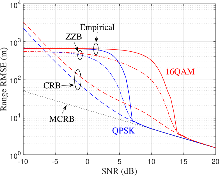
Figure 1: A comparison of the Monte Carlo empirical rmse, mcrlb, crlb, and zzb on toa estimation using a priori unknown data. Results are shown for both QPSK and 16QAM constellations.

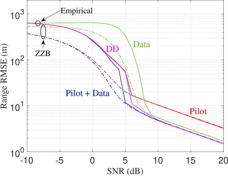
Figure 2: A comparison of the Monte Carlo empirical rmse and bounds for pilot-only, data-only, and pilot-plus-data estimation. Results are shown for a single ofdm symbol with $64$ subcarriers, QPSK modulation, and $8$ sparsely-placed pilot resources.

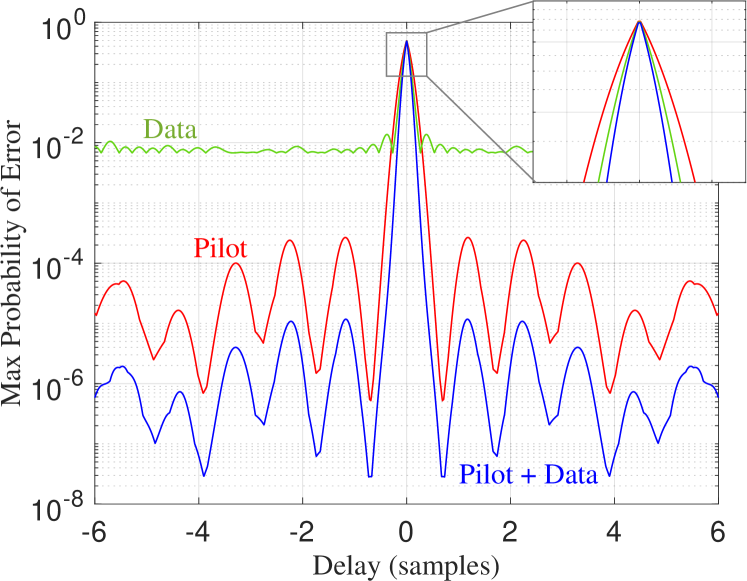
Figure 3: A plot of the maximin probability of error $\max_{\phi}\left[P_{\text{min}}(z,\phi)\right]$ against delay $z$ computed as part of the zzb in (13) for pilot-only, data-only, and pilot-plus-data estimation. Results are shown for the same signal in Fig. 2 at $5\text{\,}\mathrm{dB}$ snr.

Fig. 1 compares the derived zzb in (13), the crlb in (9), and the mcrlb in (7) on toa estimation against Monte-Carlo-simulation-based rmse assuming the data-only ml estimator in (34). The toa rmse are scaled by the speed of light and plotted in units of meters. The ofdm signal consists of $K=64$ subcarriers, $N_{\text{sym}}=1$ symbols, a subcarrier spacing of $\Delta_{\text{f}}=$15\text{\,}\mathrm{kHz}$$, and an a priori toa duration of $T_{\text{a}}=$6.25\text{\,}\mathrm{\SIUnitSymbolMicro s}$$. All $64$ resource elements are allocated as data resources. Empirical toa rmse were estimated over $20000$ Monte Carlo iterations of random noise at each snr. The grid search was conducted with intervals of $\Delta_{z}=$1/8\text{\,}$$ sample and $\Delta_{\phi}=$15\text{\,}\mathrm{\SIUnitSymbolDegree}$$.

The mcrlb is the loosest bound, only converging with the empirical rmse at high snr above $10\text{\,}\mathrm{dB}$ for QPSK and $17\text{\,}\mathrm{dB}$ for 16QAM. The crlb in (9) remains tighter than the mcrlb over a larger range of snr, capturing the slight deviation from the mcrlb above $7\text{\,}\mathrm{dB}$ snr for QPSK and $14\text{\,}\mathrm{dB}$ snr for 16QAM. Below these snr, the empirical toa errors experience the low-snr thresholding effect and rmse increase suddenly, a phenomenon not captured by the crlb. The zzb provides a much tighter bound in this thresholding regime than the mcrlb and crlb. Asymptotically as snr decreases, the zzb and empirical rmse converge to different values since the empirical toa estimator is ml, not mmse. Accordingly, the zzb rmse converges to $\sqrt{T_{\text{a}}/12}\;$\text{\,}\mathrm{s}$$, the standard deviation of a uniform distribution with duration $T_{\text{a}}\;$\text{\,}\mathrm{s}$$ [47].

Fig. 2 provides a different perspective and compares the empirical rmse against their zzb for the four types of estimators: pilot-only ml, data-only ml, pilot-plus-data ml, and dd. The ofdm signal is parameterized identically to the signal in Fig. 1 but is additionally allocated with a sparse placement of $8$ pilot resources. The pilot resource placement is optimized to minimize toa error at $0\text{\,}\mathrm{dB}$ snr using the integer-optimization routines in [38]. Power is allocated equally across all resources.

Below $8\text{\,}\mathrm{dB}$ snr, the pilot-only estimator reduces error compared to the data-only estimator. Above this snr, however, the data-only estimator reduces toa errors significantly over the pilot-only estimator, ultimately achieving an rmse of $3.0\text{\,}\mathrm{m}$ compared to the pilot-only estimator’s rmse of $5.8\text{\,}\mathrm{m}$ at $15\text{\,}\mathrm{dB}$ snr. The pilot-plus-data estimator achieves the lowest rmse across all snr. This is most notable in the thresholding regime, with the pilot-plus-data estimator achieving an rmse of $11.8\text{\,}\mathrm{m}$ compared to pilot-only rmse of $54.5\text{\,}\mathrm{m}$ and data-only rmse of $338.2\text{\,}\mathrm{m}$ at $5\text{\,}\mathrm{dB}$ snr. Meanwhile, the dd estimator is only capable of improving upon the pilot-only estimator at and above $6\text{\,}\mathrm{dB}$ snr, after which it plateaus near the same rmse as the pilot-plus-data estimator.

Fig. 3 provides insight into how the different types of estimation affect the probability of error in (16), thereby changing the zzb in (13). As seen in Fig. 2, all three zzb at $5\text{\,}\mathrm{dB}$ snr are experiencing the low-snr thresholding effect to varying degrees. At this snr, Fig. 3 shows that the pilot-only probability of error exhibits high sidelobes and a wide peak near the true delay, resulting in the large rmse in Fig. 2. Meanwhile, the data-only probability of error exhibits a sharper peak but higher sidelobes that remain relatively flat across all delays. This elevated sidelobe presence significantly increases the likelihood of toa estimates occurring outside of the mainlobe. As a result, data-only estimation has the highest rmse in Fig. 2 at $5\text{\,}\mathrm{dB}$ snr despite the sharpened mainlobe. In contrast, the pilot-plus-data probability of error exhibits both the sharpest mainlobe peak and the lowest sidelobe probability, allowing pilot-plus-data estimation to mitigate the low-snr thresholding effect significantly and achieve a lower rmse than the pilot-only and data-only estimators.

V-B Sparse Resource Optimization

Now consider the problem of allocating prs in an ofdm signal designed for both positioning and communications. To minimize the reduction in data rate, the prs will be allocated sparsely throughout the bandwidth of the signal. Consider an ofdm signal consisting of $K=240$ subcarriers, $N_{\text{sym}}=4$ symbols, a subcarrier spacing of $\Delta_{\text{f}}=$240\text{\,}\mathrm{kHz}$$, and an a priori toa duration of $T_{\text{a}}=$156.25\text{\,}\mathrm{ns}$$. Assume the subcarriers are divided into $20$ resource blocks of 12 subcarriers each, where each resource block is restricted to containing either a prs block or a data block filled with QPSK data resources. Letting $N_{\text{PRS}}$ denote the number of resource blocks that are allocated with a prs block, the allocation problem is to determine the best placement of these $N_{\text{PRS}}$ prs blocks among the $20$ available resource blocks.

Each prs block has been arbitrarily chosen to consist of pilot resources placed in a size $4$ comb pattern, similarly to the prs in 5G NR, which is visualized in Fig. 4. All non-pilot resource elements in each prs block are allocated as data resources.

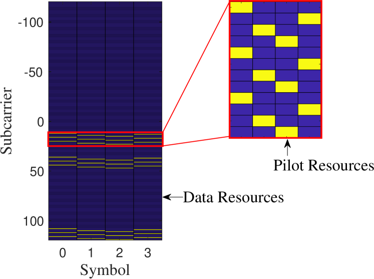
Figure 4: A visualization of the optimized ofdm resource allocation for $N_{\text{PRS}}=3$ at $0\text{\,}\mathrm{dB}$ snr.

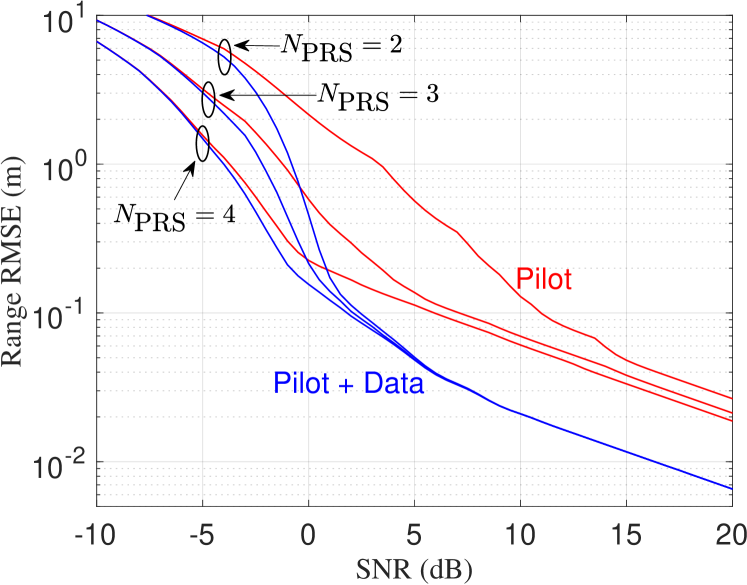
Figure 5: The zzb on toa rmse for the PRS-optimized resource allocations. Results are shown for $N_{\text{PRS}}\in\{2,3,4\}$.

The pilot-only zzb was evaluated for all permutations of prs allocation for $N_{\text{PRS}}\in\{2,3,4\}$ at each snr. The pilot-optimal allocation at each snr was then chosen as the allocation that minimized the zzb. The pilot-plus-data zzb was then evaluated on the pilot-optimal allocations. Fig. 5 plots both the pilot-only and pilot-plus-data zzb of the pilot-optimal allocations against snr. Increasing the number of prs resource blocks reduces the zzb for both pilot-only and pilot-plus-data estimation, yielding the greatest improvement at lower snr where the additional pilot resources can mitigate the low-snr thresholding effect. However, this improvement becomes negligible for the pilot-plus-data zzb above approximately $6\text{\,}\mathrm{dB}$ snr where the bounds converge. In this high snr regime, the pilot-plus-data zzb show significant reductions in error compared to the pilot-only zzb. At $10\text{\,}\mathrm{dB}$ snr, all three pilot-plus-data zzb have a rmse of $2.1\text{\,}\mathrm{cm}$ compared to rmse of $6.1\text{\,}\mathrm{cm}$, $7.0\text{\,}\mathrm{cm}$, and $12.9\text{\,}\mathrm{cm}$ for the pilot-only zzb. Into low snr, the pilot-plus-data zzb still show notable improvements over their respective pilot-only zzb even though the prs allocations are optimized for pilot-only estimation at every snr.

V-C LEO Satellite Positioning

Positioning with leo satellite downlink signals is a particularly apt application for the ml and dd toa estimators discussed in Section IV. leo channels can span wide bandwidths, enabling highly-accurate toa estimates and therefore accurate user positioning services. Furthermore, leo channels experience minimal fading especially when combined with highly-directional phased arrays at both the transmitter and receiver, resulting in flat channel responses across the wide signal bandwidths. Finally, leo satellites provide communication services to large cells which are likely to contain many network users, increasing the amount of downlink data resources that will need to be allocated. If the leo satellites transmit in bursts to manage power consumption [2], downlink resources are likely to be fully allocated to maximize throughput. One example is the downlink Starlink signal which consists of frames with fully allocated data [14]. In such a fully allocated burst, the allocation of prs comes at the cost of decreased throughput. Therefore, it may be beneficial to allocate fewer resources to positioning services and instead have receivers exploit the unknown data resources to obtain accurate positioning. In this section, the positioning performance of the ml and dd toa estimators is evaluated on a simulated leo downlink channel.

Setup

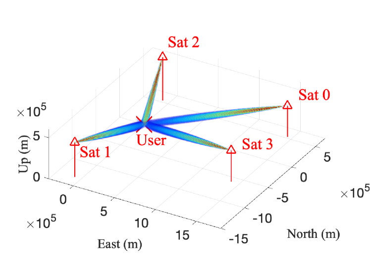
Figure 6: A visualization of the four satellites in the simulated LEO constellation and each satellite’s downlink beam.

The simulated environment consists of four leo satellites and one receiver. The receiver’s cell receives downlink service from each satellite in a time-duplexed manner with the interval between downlink bursts from each satellite denoted as $T_{\text{burst}}$. During each downlink burst, the servicing satellite directs its beam to the center of the cell and pre-compensates for the expected Doppler shift experienced by a stationary user at the center of the cell. For simplicity, the receiver is stationary and located at the center of its cell. The receiver also has perfect knowledge of each satellite’s relative position and applies conventional beamforming weights to its phased array elements to direct its beam in the known direction of the servicing satellite. Fig. 6 shows a graphical depiction of the simulation setup and the downlink beams.

Each burst consists of $N_{\text{sym}}=4$ ofdm symbols. The ofdm signal parameters and simulation parameters are listed in Table I. Simulated frequency-selective, time-varying channels are generated using QuaDRiGa [48]. Two channel models are considered: QuaDRiGa_NTN_DenseUrban_LOS [49] and 5G-ALLSTAR_DenseUrban_LOS [50].

For each channel model, $1000$ channel realizations were generated. For each channel realization, $1000$ realizations of awgn were generated. Pseudorange estimates were obtained for each channel and awgn realization using each of the estimators Additionally, the zzb was computed for each channel realization.

Let $\bm{r}_{i}$ be the enu coordinates of satellite $i$ for $i\in\{0,1,2,3\}$, $\bm{r}$ be the enu coordinates of the receiver, and $\delta_{t}$ be the clock offset between the receiver and the satellite constellation. Define $c$ as the speed of light, $\bm{\epsilon}_{\rho}$ as pseudorange estimation error, and $\bm{\theta}_{\rho}\triangleq[\bm{r}^{T},\;c\delta_{t}]^{T}$. Additionally define

$$h_{i}(\bm{\theta}_{\rho})\triangleq c||\bm{r}_{i}-\bm{r}||+c\delta_{t},$$ (38)

which is expressed in vector form as $\bm{h}(\bm{\theta}_{\rho})\triangleq[h_{0}(\bm{\theta}_{\rho}),\;h_{1}(\bm{\theta}_{\rho}),\;h_{2}(\bm{\theta}_{\rho}),\;h_{3}(\bm{\theta}_{\rho})]^{T}$. Then the vectorized pseudorange measurement equation for all satellites becomes

$$\bm{\rho}=\bm{h}(\bm{\theta}_{\rho})+\bm{\epsilon}_{\rho}.$$ (39)

Letting $\bm{\Sigma}_{\bm{\rho}}$ be the covariance of the pseudorange error $\bm{\epsilon}_{\rho}$, a positioning solution can then be obtained by solving the weighted nonlinear least-squares problem:

$$\hat{\bm{\theta}}_{\rho}=\operatorname*{\arg\!\min}_{\bm{\theta}_{\rho}}\bigl{|}\bigl{|}\bm{\rho}-\bm{h}(\bm{\theta}_{\rho})\bigr{|}\bigr{|}_{\bm{\Sigma}_{\bm{\rho}}^{-1}}^{2}.$$ (40)

The error covariance of this estimate can be approximated by linearizing the pseudorange residuals at the true values of $\bm{\theta}_{\rho}$. Defining the matrix

$$\bm{A}\triangleq\begin{bmatrix}\textstyle\frac{\bm{r}_{0}-\bm{r}}{||\bm{r}_{0}-\bm{r}||^{2}}&\textstyle\frac{\bm{r}_{1}-\bm{r}}{||\bm{r}_{1}-\bm{r}||^{2}}&\textstyle\frac{\bm{r}_{2}-\bm{r}}{||\bm{r}_{2}-\bm{r}||^{2}}&\textstyle\frac{\bm{r}_{3}-\bm{r}}{||\bm{r}_{3}-\bm{r}||^{2}}\\ 1&1&1&1\end{bmatrix}^{T},$$ (41)

the error covariance of $\hat{\bm{\theta}}_{\rho}$ can then be described as $\bm{Q}\triangleq\left(\bm{A}^{T}\bm{\Sigma}_{\bm{\rho}}^{-1}\bm{A}\right)^{-1}$. The diagonal elements of this error covariance are defined as $[\sigma_{x}^{2},\;\sigma_{y}^{2},\;\sigma_{z}^{2},\;\sigma_{c\delta{t}}^{2}]^{T}\triangleq\text{diag}(\bm{Q})$.

Since each pseudorange is obtained independently, $\bm{\Sigma}_{\bm{\rho}}$ is a diagonal matrix consisting of elements $\sigma_{\rho_{0}}^{2}$, $\sigma_{\rho_{1}}^{2}$, $\sigma_{\rho_{2}}^{2}$, and $\sigma_{\rho_{3}}^{2}$. These variances are obtained either from the zzb or from the empirical error variance of the toa estimates over awgn realizations for a single channel realization. It is important to note that the distribution of the toa errors is unknown and not guaranteed to be Gaussian. However, the zzb and empirical error variances can be compared through this linearized model.

TABLE I: LEO Simulation Parameters

OFDM Parameters
$K$	$240$ subcarriers
$\Delta_{\text{f}}$ (Subcarrier Spacing)	$240\text{\,}\mathrm{kHz}$
Symbol Duration	$4.167\text{\,}\mathrm{\SIUnitSymbolMicro s}$
Cyclic Prefix Duration	$0.521\text{\,}\mathrm{\SIUnitSymbolMicro s}$
Bandwidth	$57.60\text{\,}\mathrm{MHz}$
Symbol Constellation	QPSK
Simulation Parameters
$f_{\text{c}}$ (Carrier Frequency)	$10.7\text{\,}\mathrm{GHz}$
Polarization	LHCP @ RX & TX
TX Gain	$34\text{\,}\mathrm{dB}$
TX Beamwidth	$3.67\text{\,}\mathrm{\SIUnitSymbolDegree}$
RX Array	$32\times 32$ URA $\left(\lambda/2\;\text{spacing}\right)$
RX Gain	$30\text{\,}\mathrm{dB}$
RX Beamwidth	$3.58\text{\,}\mathrm{\SIUnitSymbolDegree}$
EIRP	$-15\text{\,}\mathrm{d}\mathrm{B}\mathrm{W}\mathrm{/}\mathrm{4}\mathrm{k}\mathrm{Hz}$
$\sigma^{2}$ (Resource Noise Power)	$-173.8+10\log_{10}(\Delta_{\text{f}})$ $\text{\,}\mathrm{dBm}$
$T_{\text{a}}$ (a priori toa Duration)	$156.25\text{\,}\mathrm{ns}$
$T_{\text{burst}}$ (Burst Interval)	$1\text{\,}\mathrm{ms}$
Satellite Altitude	$550\text{\,}\mathrm{km}$
Satellite Constellation	Walker-Delta $53\text{\,}\mathrm{\SIUnitSymbolDegree}$:1584/22/39
Elevation Mask	$30\text{\,}\mathrm{\SIUnitSymbolDegree}$
Channel Models	QuaDRiGa_NTN_DenseUrban_LOS
	5G-ALLSTAR_DenseUrban_LOS

LEO Results

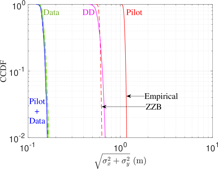
Figure 7: The ccdf of horizontal rmse over channel realizations using the QuaDRiGa channel model, comparing the pilot-only, data-only, pilot-plus-data, and dd estimators. Results are shown for both the zzb and empirical data.

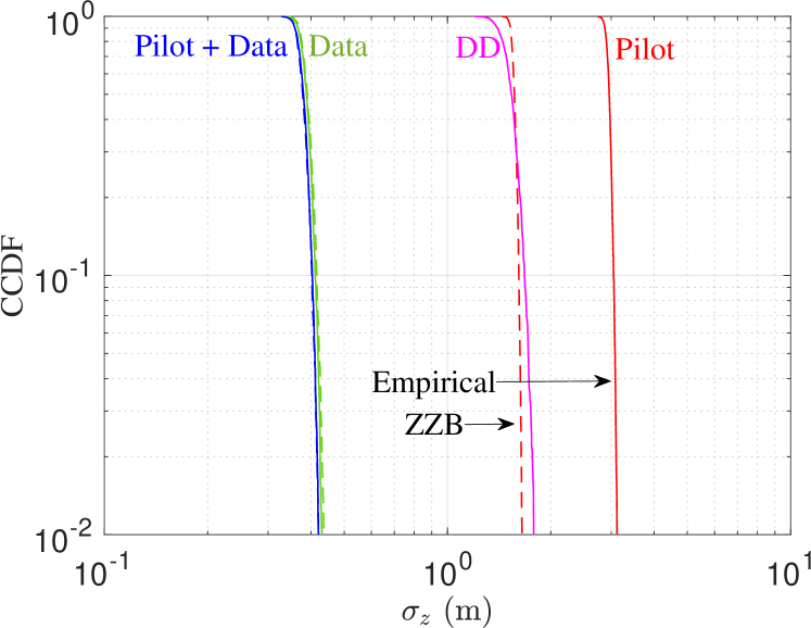
Figure 8: As Fig. 7 but for vertical rmse.

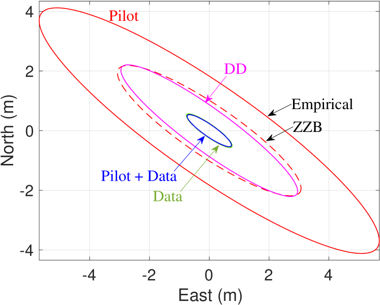
Figure 9: The $95\text{\,}\mathrm{\char 37\relax}$ horizontal positioning error ellipses for the QuaDRiGa channel model. Results are obtained using the Chebyshev inequality with both the zzb and empirical rmse over all channel realizations.

Fig. 7 and Fig. 8 plot the ccdf over channel realizations of the horizontal rmse and vertical rmse using the QuaDRiGa_NTN_DenseUrban_LOS channel model. Both the zzb and empirical rmse are depicted for each of the estimators. The pilot-only estimator results in the greatest errors, having a $90$th percentile horizontal rmse of $1.15\text{\,}\mathrm{m}$ and vertical rmse of $3.05\text{\,}\mathrm{m}$. The decision-directed estimator yields moderate improvements over the pilot-only estimator, having a $90$th percentile horizontal rmse of $0.64\text{\,}\mathrm{m}$ and vertical rmse of $1.68\text{\,}\mathrm{m}$. Accuracy is improved significantly with the data-only estimator, having a $90$th percentile horizontal rmse of $0.16\text{\,}\mathrm{m}$ and vertical rmse of $0.41\text{\,}\mathrm{m}$. Finally, the pilot-plus-data estimator achieves the best accuracy, having a $90$th percentile horizontal rmse of $0.15\text{\,}\mathrm{m}$ and vertical rmse of $0.40\text{\,}\mathrm{m}$.

Fig. 9 provides an alternative depiction of these results, visualizing the $95\text{\,}\mathrm{\char 37\relax}$ error ellipses using both the zzb and empirical rmse over all channel realizations. Since the error distribution is not guaranteed to be Gaussian, the $95\text{\,}\mathrm{\char 37\relax}$ error ellipses are computed using the multivariate Chebyshev inequality [51], resulting in a 2D ellipse corresponding to $6.32$ standard deviations. The Chebyshev inequality allows confidence intervals to be constructed for any arbitrary distribution with a finite variance. This depiction highlights how the data-only and pilot-plus-data estimators reduce positioning error significantly compared to the pilot-only estimator and even the dd estimator. The data-only and pilot-plus-data ellipses have a semi-major axis of approximately $0.9\text{\,}\mathrm{m}$ compared to the dd ellipse’s $3.6\text{\,}\mathrm{m}$ and pilot-only ellipse’s $6.9\text{\,}\mathrm{m}$. The zzb ellipses are nearly coincident with the empirical ellipses for data-only and pilot-plus-data estimation, while the zzb ellipse for pilot-only estimation has a gap compared to the empirical ellipse and a semi-major axis of $3.7\text{\,}\mathrm{m}$.

The pilot-plus-data and data-only estimators are capable of outperforming the pilot-only estimator by exploiting significantly more resources in the signal. Compared to the DD estimator, these estimators are not negatively impacted by errors in the hard decoding process. As a result, the DD estimator requires much higher snr to approach the performance of the pilot-plus-data and data-only estimators.

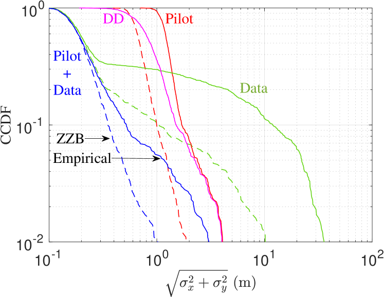
Figure 10: The ccdf over channel realizations of horizontal rmse using the 5G-ALLSTAR channel model, comparing the pilot-only, data-only, pilot-plus-data, and dd estimators. Results are shown for both the zzb and empirical data.

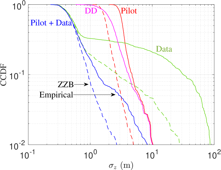
Figure 11: As Fig. 10 but for vertical rmse.

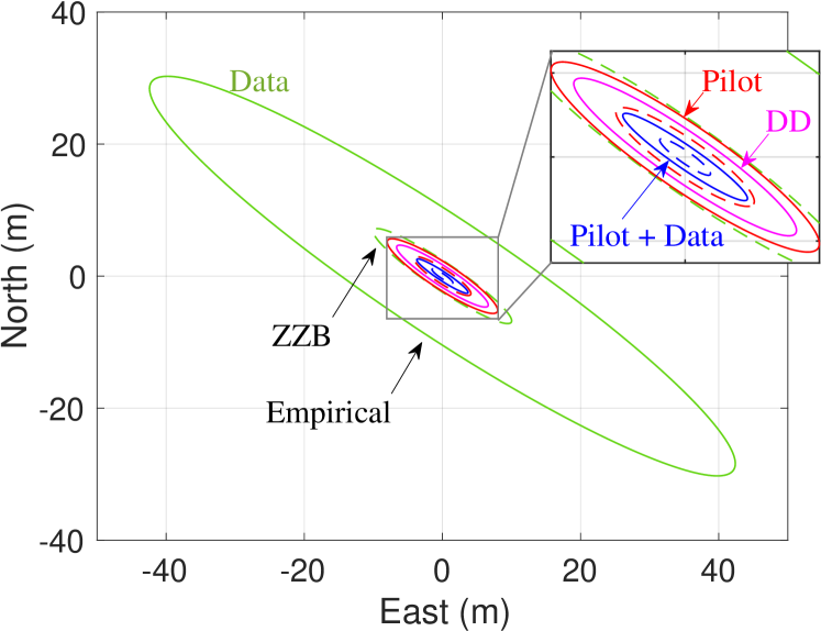
Figure 12: The $95\text{\,}\mathrm{\char 37\relax}$ horizontal positioning error ellipses for the 5G-ALLSTAR channel model. Results are obtained using the Chebyshev inequality with both the zzb and empirical rmse over all channel realizations.

Figs. 10 and 11 plot the ccdf over channel realizations of the horizontal rmse and vertical rmse using the 5G-ALLSTAR_DenseUrban_LOS channel model, similar to Figs. 7 and 8. Different patterns emerge with this channel model, as greater fluctuations in snr are simulated. Similar to the results in Figs. 7 and 8, the pilot-plus-data estimator achieves the greatest accuracy, having a $90$th percentile horizontal rmse of $0.52\text{\,}\mathrm{m}$ and vertical rmse of $1.32\text{\,}\mathrm{m}$. However, the data-only estimator only outperforms the DD and pilot-only estimators in approximately $70\text{\,}\mathrm{\char 37\relax}$ of channel realizations. In the remaining $30\text{\,}\mathrm{\char 37\relax}$ of channel realizations, the low snr cause the data-only estimator to enter its thresholding regime, resulting in rmse surpassing those achieved using only pilots. The data-only estimator has a $90$th percentile horizontal rmse of $11.96\text{\,}\mathrm{m}$ and vertical rmse of $32.00\text{\,}\mathrm{m}$. Meanwhile, the dd estimator exhibits less improvement over the pilot-only estimator in this channel model, having a $90$th percentile horizontal rmse of $1.52\text{\,}\mathrm{m}$ and vertical rmse of $4.16\text{\,}\mathrm{m}$ compared to the pilot-only estimator’s $90$th percentile horizontal rmse of $1.71\text{\,}\mathrm{m}$ and vertical rmse of $4.73\text{\,}\mathrm{m}$.

Fig. 12 visualizes the $95\text{\,}\mathrm{\char 37\relax}$ error ellipses for the 5G-ALLSTAR channel model, similar to Fig. 9. As with the results in Fig. 10 and Fig. 11, the data-only estimator exhibits significant errors due to the poor channel conditions. Meanwhile, the pilot-plus-data estimator reduces postioning error compared to both the pilot-only and dd estimators. The pilot-plus-data ellipse has a semi-major axis of approximately $4.5\text{\,}\mathrm{m}$ compared to the dd ellipse’s $8.0\text{\,}\mathrm{m}$, pilot-only ellipse’s $9.6\text{\,}\mathrm{m}$, and data-only ellipse’s $52\text{\,}\mathrm{m}$.

The large snr fluctuations in the 5G-ALLSTAR_DenseUrban_LOS channel model resulted in the estimators entering their low-snr thresholding regimes. The pilot-plus-data estimator provides robustness against these thresholding effects at low snr while simultaneously maximizing accuracy in high snr. In comparison to Fig. 7 and Fig. 8, the zzb are much looser due to the bound not being as tight in the low-snr thresholding regime as in the high-snr regime.

VI Conclusions

This paper has derived a novel zzb on toa estimation with ofdm signals containing unknown data resources. This zzb serves as a lower bound to both ml and dd estimators that can exploit unknown data resources to improve estimation accuracy. The zzb was shown to be tighter to empirical errors than the crlb and mcrlb derived in prior work, making it a useful criterion for evaluating different ofdm resource allocations for toa estimation. Comparisons were then made between four different types of estimators: pilot-only ml, data-only ml, pilot-plus-data ml, and dd, demonstrating that the pilot-plus-data estimator can significantly improve toa estimation accuracy. The zzb was then used to evaluate different allocations of prs within a wideband ofdm signal, which can guide resource allocations that minimize overhead while still achieving toa accuracy requirements. Finally, the zzb and toa estimators were evaluated on simulated leo channels, quantifying the distribution of positioning rmse across channel realizations. These results highlight the potential for ofdm networks to significantly improve positioning performance while still prioritizing data throughput.

References

- [1] H. K. Dureppagari, C. Saha, H. S. Dhillon, and R. M. Buehrer, “NTN-based 6G localization: Vision, role of LEOs, and open problems,” IEEE Wireless Communications, vol. 30, no. 6, pp. 44–51, 2023.
- [2] P. A. Iannucci and T. E. Humphreys, “Fused low-earth-orbit GNSS,” IEEE Transactions on Aerospace and Electronic Systems, pp. 1–1, 2022.
- [3] X. Lin, S. Cioni, G. Charbit, N. Chuberre, S. Hellsten, and J.-F. Boutillon, “On the path to 6G: Embracing the next wave of low Earth orbit satellite access,” IEEE Communications Magazine, vol. 59, no. 12, pp. 36–42, 2021.
- [4] S. Dwivedi, R. Shreevastav, F. Munier, J. Nygren, I. Siomina, Y. Lyazidi, D. Shrestha, G. Lindmark, P. Ernström, E. Stare et al., “Positioning in 5G networks,” IEEE Communications Magazine, vol. 59, no. 11, pp. 38–44, 2021.
- [5] A. M. Graff and T. E. Humphreys, “Purposeful co-design of OFDM signals for ranging and communications,” EURASIP Journal on Advances in Signal Processing, 2024.
- [6] F. Bellili, N. Atitallah, S. Affes, and A. Stéphenne, “Cramér-Rao lower bounds for frequency andphase NDA estimation from arbitrary square QAM-modulated signals,” IEEE Transactions on Signal Processing, vol. 58, no. 9, pp. 4517–4525, 2010.
- [7] A. Masmoudi, F. Bellili, S. Affes, and A. Stephenne, “A non-data-aided maximum likelihood time delay estimator using importance sampling,” IEEE Transactions on Signal Processing, vol. 59, no. 10, pp. 4505–4515, 2011.
- [8] A. Zeira and P. M. Schultheiss, “Realizable lower bounds for time delay estimation. 2. Threshold phenomena,” IEEE transactions on signal processing, vol. 42, no. 5, pp. 1001–1007, 1994.
- [9] J. A. Nanzer, M. D. Sharp, and D. Richard Brown, “Bandpass signal design for passive time delay estimation,” in 2016 50th Asilomar Conference on Signals, Systems and Computers, Nov. 2016, pp. 1086–1091.
- [10] Z. Sahinoglu, S. Gezici, and I. Güvenc, Ultra-wideband positioning systems: theoretical limits, ranging algorithms, and protocols. Cambridge university press, 2008.
- [11] E. W. Barankin, “Locally best unbiased estimates,” The Annals of Mathematical Statistics, vol. 20, no. 4, pp. 477–501, 1949. [Online]. Available: http://www.jstor.org/stable/2236306
- [12] R. McAulay and E. Hofstetter, “Barankin bounds on parameter estimation,” IEEE Transactions on Information Theory, vol. 17, no. 6, pp. 669–676, 1971.
- [13] J. Ziv and M. Zakai, “Some lower bounds on signal parameter estimation,” IEEE Transactions on Information Theory, vol. 15, no. 3, pp. 386–391, 1969.
- [14] T. E. Humphreys, P. A. Iannucci, Z. M. Komodromos, and A. M. Graff, “Signal structure of the Starlink Ku-band downlink,” IEEE Transactions on Aerospace and Electronic Systems, pp. 1–16, 2023.
- [15] M. Koivisto, M. Costa, J. Werner, K. Heiska, J. Talvitie, K. Leppänen, V. Koivunen, and M. Valkama, “Joint device positioning and clock synchronization in 5G ultra-dense networks,” IEEE Transactions on Wireless Communications, vol. 16, no. 5, pp. 2866–2881, 2017.
- [16] A. Kakkavas, H. Wymeersch, G. Seco-Granados, M. H. C. García, R. A. Stirling-Gallacher, and J. A. Nossek, “Power allocation and parameter estimation for multipath-based 5G positioning,” IEEE Transactions on Wireless Communications, vol. 20, no. 11, pp. 7302–7316, 2021.
- [17] K. Shamaei and Z. M. Kassas, “LTE receiver design and multipath analysis for navigation in urban environments,” Navigation, vol. 65, no. 4, pp. 655–675, 2018.
- [18] ——, “Receiver design and time of arrival estimation for opportunistic localization with 5G signals,” IEEE Transactions on Wireless Communications, vol. 20, no. 7, pp. 4716–4731, 2021.
- [19] M. Neinavaie, J. Khalife, and Z. M. Kassas, “Cognitive opportunistic navigation in private networks with 5G signals and beyond,” IEEE Journal of Selected Topics in Signal Processing, vol. 16, no. 1, pp. 129–143, 2021.
- [20] M. Neinavaie and Z. M. Kassas, “Cognitive sensing and navigation with unknown OFDM signals with application to terrestrial 5G and Starlink LEO satellites,” IEEE Journal on Selected Areas in Communications, 2023.
- [21] H. Xv, Y. Sun, Y. Zhao, M. Peng, and S. Zhang, “Joint beam scheduling and beamforming design for cooperative positioning in multi-beam LEO satellite networks,” IEEE Transactions on Vehicular Technology, 2023.
- [22] K. Shi, E. Serpedin, and P. Ciblat, “Decision-directed fine synchronization in OFDM systems,” IEEE Transactions on Communications, vol. 53, no. 3, pp. 408–412, 2005.
- [23] J. Ran, R. Grunheid, H. Rohling, E. Bolinth, and R. Kern, “Decision-directed channel estimation method for OFDM systems with high velocities,” in The 57th IEEE Semiannual Vehicular Technology Conference, 2003. VTC 2003-Spring., vol. 4. IEEE, 2003, pp. 2358–2361.
- [24] E. Karami and M. Shiva, “Decision-directed recursive least squares MIMO channels tracking,” EURASIP Journal on Wireless Communications and Networking, vol. 2006, pp. 1–10, 2006.
- [25] Y. Xiong, L. Tang, S. Sun, L. Liu, S. Mao, Z. Zhang, and N. Wei, “Data-aided channel estimation and combining for cell-free massive MIMO with low-resolution ADCs,” IEEE Communications Letters, 2024.
- [26] X. Ma, C. Tepedelenlioglu, G. B. Giannakis, and S. Barbarossa, “Non-data-aided carrier offset estimators for OFDM with null subcarriers: identifiability, algorithms, and performance,” IEEE Journal on selected areas in communications, vol. 19, no. 12, pp. 2504–2515, 2001.
- [27] A. Al-Dweik, “A novel non-data-aided symbol timing recovery technique for OFDM systems,” IEEE Transactions on Communications, vol. 54, no. 1, pp. 37–40, 2006.
- [28] F.-X. Socheleau, A. Aissa-El-Bey, and S. Houcke, “Non data-aided SNR estimation of OFDM signals,” IEEE communications letters, vol. 12, no. 11, pp. 813–815, 2008.
- [29] A. Masmoudi, F. Bellili, S. Affes, and A. Stéphenne, “Closed-form expressions for the exact Cramér–Rao bounds of timing recovery estimators from BPSK, MSK and square-QAM transmissions,” IEEE transactions on signal processing, vol. 59, no. 6, pp. 2474–2484, 2011.
- [30] A. Masmoudi, F. Bellili, S. Affes, and A. Ghrayeb, “Maximum likelihood time delay estimation from single- and multi-carrier DSSS multipath MIMO transmissions for future 5G networks,” IEEE Transactions on Wireless Communications, vol. 16, no. 8, pp. 4851–4865, 2017.
- [31] S. Monfared, T.-H. Nguyen, T. Van der Vorst, P. De Doncker, and F. Horlin, “Iterative NDA positioning using angle-of-arrival measurements for IoT sensor networks,” IEEE Transactions on Vehicular Technology, vol. 69, no. 10, pp. 11 369–11 382, 2020.
- [32] W. Wang, T. Jost, C. Gentner, S. Zhang, and A. Dammann, “A semiblind tracking algorithm for joint communication and ranging with OFDM signals,” IEEE Transactions on Vehicular Technology, vol. 65, no. 7, pp. 5237–5250, 2015.
- [33] R. Adam and P. A. Hoeher, “Semi-blind channel estimation for joint communication and positioning,” in 2013 10th Workshop on Positioning, Navigation and Communication (WPNC). IEEE, 2013, pp. 1–5.
- [34] C. Mensing, S. Sand, A. Dammann, and W. Utschick, “Data-aided location estimation in cellular OFDM communications systems,” in GLOBECOM 2009 - 2009 IEEE Global Telecommunications Conference, 2009, pp. 1–7.
- [35] T. Laas and W. Xu, “On the Ziv-Zakai bound for time difference of arrival estimation in CP-OFDM systems,” in 2021 IEEE Wireless Communications and Networking Conference (WCNC). IEEE, 2021, pp. 1–5.
- [36] A. Dammann, T. Jost, R. Raulefs, M. Walter, and S. Zhang, “Optimizing waveforms for positioning in 5G,” in 2016 IEEE 17th International Workshop on Signal Processing Advances in Wireless Communications (SPAWC). IEEE, 2016, pp. 1–5.
- [37] E. Staudinger, M. Walter, and A. Dammann, “Optimized waveform for energy efficient ranging,” in 2017 14th Workshop on Positioning, Navigation and Communications (WPNC). IEEE, 2017, pp. 1–6.
- [38] A. M. Graff and T. E. Humphreys, “Ziv-Zakai-optimal OFDM resource alocation for time-of-arrival estimation,” IEEE Transactions on Wireless Communications, 2024, submitted for review.
- [39] A. Gusi-Amigó, P. Closas, A. Mallat, and L. Vandendorpe, “Ziv-Zakai bound for direct position estimation,” Navigation, vol. 65, no. 3, pp. 463–475, 2018.
- [40] W. Xu, M. Huang, C. Zhu, and A. Dammann, “Maximum likelihood TOA and OTDOA estimation with first arriving path detection for 3GPP LTE system,” Transactions on Emerging Telecommunications Technologies, vol. 27, no. 3, pp. 339–356, 2016.
- [41] A. N. D’Andrea, U. Mengali, and R. Reggiannini, “The modified Cramer-Rao bound and its application to synchronization problems,” IEEE Transactions on Communications, vol. 42, no. 234, pp. 1391–1399, 1994.
- [42] S. Bellini and G. Tartara, “Bounds on error in signal parameter estimation,” IEEE Transactions on Communications, vol. 22, no. 3, pp. 340–342, 1974.
- [43] K. L. Bell, Y. Steinberg, Y. Ephraim, and H. L. Van Trees, “Extended Ziv-Zakai lower bound for vector parameter estimation,” IEEE Transactions on information theory, vol. 43, no. 2, pp. 624–637, 1997.
- [44] N. B. Mehta, J. Wu, A. F. Molisch, and J. Zhang, “Approximating a sum of random variables with a lognormal,” IEEE Transactions on Wireless Communications, vol. 6, no. 7, pp. 2690–2699, 2007.
- [45] M. Abramowitz and I. A. Stegun, Handbook of mathematical functions with formulas, graphs, and mathematical tables. US Government printing office, 1968, vol. 55.
- [46] D. Dardari and M. Z. Win, “Ziv-Zakai bound on time-of-arrival estimation with statistical channel knowledge at the receiver,” in 2009 IEEE International Conference on Ultra-Wideband. IEEE, 2009, pp. 624–629.
- [47] D. Chazan, M. Zakai, and J. Ziv, “Improved lower bounds on signal parameter estimation,” IEEE transactions on Information Theory, vol. 21, no. 1, pp. 90–93, 1975.
- [48] F. Burkhardt, S. Jaeckel, E. Eberlein, and R. Prieto-Cerdeira, “QuaDRiGa: A MIMO channel model for land mobile satellite,” in The 8th European Conference on Antennas and Propagation (EuCAP 2014). IEEE, 2014, pp. 1274–1278.
- [49] S. Jaeckel, L. Raschkowski, and L. Thieley, “A 5G-NR satellite extension for the QuaDRiGa channel model,” in 2022 Joint European Conference on Networks and Communications & 6G Summit (EuCNC/6G Summit). IEEE, 2022, pp. 142–147.
- [50] N. Cassiau, G. Noh, S. Jaeckel, L. Raschkowski, J.-M. Houssin, L. Combelles, M. Thary, J. Kim, J.-B. Dore, and M. Laugeois, “Satellite and terrestrial multi-connectivity for 5G: Making spectrum sharing possible,” in 2020 IEEE Wireless Communications and Networking Conference Workshops (WCNCW). IEEE, 2020, pp. 1–6.
- [51] A. W. Marshall and I. Olkin, “Multivariate chebyshev inequalities,” The Annals of Mathematical Statistics, pp. 1001–1014, 1960.