Gürlek, de Véricourt, and Lee

Boosted Generalized Normal Distributions

Boosted Generalized Normal Distributions: Integrating Machine Learning with Operations Knowledge

Ragıp Gürlek Goizueta Business School, Emory University

Francis de Véricourt European School of Management and Technology Berlin

Donald K.K. Lee Goizueta Business School and Department of Biostatistics & Bioinformatics, Emory University

Applications of machine learning (ML) techniques to operational settings often face two challenges: i) ML methods mostly provide point predictions whereas many operational problems require distributional information; and ii) They typically do not incorporate the extensive body of knowledge in the operations literature, particularly the theoretical and empirical findings that characterize specific distributions. We introduce a novel and rigorous methodology, the Boosted Generalized Normal Distribution (bGND), to address these challenges. The Generalized Normal Distribution (GND) encompasses a wide range of parametric distributions commonly encountered in operations, and bGND leverages gradient boosting with tree learners to flexibly estimate the parameters of the GND as functions of covariates. We establish bGND’s statistical consistency, thereby extending this key property to special cases studied in the ML literature that lacked such guarantees. Using data from a large academic emergency department in the United States, we show that the distributional forecasting of patient wait and service times can be meaningfully improved by leveraging findings from the healthcare operations literature. Specifically, bGND performs 6% and 9% better than the distribution-agnostic ML benchmark used to forecast wait and service times respectively. Further analysis suggests that these improvements translate into a 9% increase in patient satisfaction and a 4% reduction in mortality for myocardial infarction patients. Our work underscores the importance of integrating ML with operations knowledge to enhance distributional forecasts.

Distributional Machine Learning, Gradient Boosting, Wait Times, Service Times, Emergency Departments, Healthcare Operations 1 August 2024

1 Introduction

Machine learning (ML) is increasingly being implemented across various areas of operations, including forecasting patient wait times in emergency departments (Arora et al. 2023), developing chemotherapy treatments (Bertsimas et al. 2016), manufacturing process improvements (Senoner et al. 2022), to optimizing last-mile delivery assignments (Liu et al. 2021). The growing application of these methodologies can be attributed to their ability to learn complex relationships, their remarkable versatility, and the increased availability of operations-related data.

However, there are two challenges to applying ML techniques to operational settings. First, the majority of ML methods provide point predictions rather than distributional forecasts. Yet, many fundamental operations problems are framed around probability distributions: The analysis of service systems, for instance, focus on the distributions of wait and service times, while the newsvendor problem requires a specific quantile of the demand distribution. Consider also staffing (He et al. 2012, Ban and Rudin 2019) and elective surgery scheduling (Rath et al. 2017), which rely on distributional estimates of hospital workload and surgery duration.

Second, the distributional ML algorithms do not account for the extensive body of knowledge in operations (Arora et al. 2023, Bertsimas et al. 2022). This is because nonparametric ML algorithms are distribution-agnostic by design, precluding them from taking advantage of the specific distributional knowledge identified in the theoretical and empirical operations literature. For instance, Kingman (1962) demonstrated that wait times in queuing systems under heavy traffic can be approximated by an exponential distribution, and empirical evidence suggests this holds even in less heavily loaded systems (Brown et al. 2005). The empirical queuing literature also established that service duration in various operations settings can be approximated by a log-normal distribution (Brown et al. 2005, He et al. 2012, Armony et al. 2015, Ding et al. 2024). The distributional ML algorithms currently used in operational contexts overlook this knowledge, which can potentially be exploited for performance gains.

In this paper, we introduce a novel distributional ML approach called the boosted Generalized Normal Distribution (bGND) to address both challenges. The classical Generalized Normal Distribution (GND) encompasses or closely approximates a wide range of parametric distributions commonly encountered in operational settings. Our proposed bGND employs an ML method called gradient boosting (Friedman 2001) to estimate the location and scale parameters of the GND as flexible functions of covariates using regression tree learners. Thus bGND combines the flexibility of ML with operations domain knowledge. Besides being the first time that the GND has been studied from an ML perspective, we also provide the first proof for bGND’s statistical consistency. This result automatically extends to all special cases of the bGND studied in the ML literature (Duan et al. 2020, März and Kneib 2022), for which no consistency results have been established.

Our motivating application comes from forecasting patient wait and service times in emergency departments (ED), an important question in healthcare operations (Shi et al. 2016, Song et al. 2015, Chan et al. 2017, Niewoehner III et al. 2023, Chen et al. 2023). In particular, Arora et al. (2023) pioneers the case for distributional forecasts over point predictions, and is the only study to provide one for wait times. They use Quantile Regression Forests (QRF) (Meinshausen 2006) to obtain the forecasts, which is a popular nonparametric distributional ML technique. By leveraging operations knowledge, we show that bGND outperforms QRF on data from a large academic ED in the United States. Specifically, using the exponential case of bGND for wait times and the log-normal case for service times, bGND outperforms by 6.1% and 8.8% on the Continuous Ranked Probability Score (CRPS) for out-of-sample wait and service time forecasts, respectively (see Table 1). Further analysis shows that these improvements translate into a 9.4% increase in patient satisfaction and a 4.1% reduction in mortality for myocardial infarction patients, respectively (see 9 in the electronic companion for details).

Perhaps more fundamentally, our approach highlights the value of incorporating operations domain knowledge: Using classic statistical models without any ML, the linearly-specified exponential and log-normal models already outperform QRF by 2.5% and 7.0% respectively in CRPS accuracy for patient wait and service times forecasts (Table 1). To our knowledge, this paper is the first to articulate and show that simple models equipped with operations knowledge can outperform nonparametric ML methods. The fact that bGND outperforms both the classical parametric models as well as QRF further demonstrates the value of combining ML techniques with operations domain knowledge in distributional forecasts.

Table 1: %Reduction in wait and service time CRPS values relative to QRF

	Wait times				Service times
	2017	2018	2019	Aggregate	2017	2018	2019	Aggregate
bGND	4.3%	8.3%	5.7%	6.1%	6.9%	7.4%	13%	8.8%
Classic exponential/log-normal	0.95%	5.1%	1.3%	2.5%	5.7%	6.7%	9.0%	7.0%

In terms of methodological contribution, while procedures exist for fitting special cases of the bGND such as the boosted normal distribution (Duan et al. 2020, März and Kneib 2022), their statistical consistency have not been studied. A possible reason is that these procedures work by jointly minimizing the negative log-likelihood (the loss) over both the location and scale parameters via gradient descent. However, the population version of the loss is non-convex even for the normal distribution (see 7 in the electronic companion for a numerical example). In addition, these procedures encounter computational issues when the log-likelihood is non-differentiable, as is the case with the Laplace distribution, which is a special case of GND. In such scenarios, the likelihood is not smooth in the location parameter, leading to numerical convergence failures.

In contrast, we employ a natural insight from traditional statistics that decouples the estimation into two separate smooth convex problems: First we estimate the location parameter as the conditional mean, and then plug in that estimate to estimate the scale parameter. This mirrors how the mean and standard deviation are traditionally estimated. Moreover, this decoupling allows us to establish the consistency of bGND, and hence the boosted normal and Laplace distributions as well. In this sense, our approach adds both computational and theoretical value to the literature.

Finally, we also contribute to the growing literature that integrates operations concepts into machine learning. Recent studies propose data-driven optimization frameworks that consider the structure of the final optimization problem during parameter estimation. Some approaches are applicable to general contexts, such as problems with linear objective and constraints (Bertsimas and Kallus 2020, Elmachtoub and Grigas 2022), while others focus on specific problems like the newsvendor problem (Ban and Rudin 2019, Notz and Pibernik 2022, Alley et al. 2023, Singh et al. 2024). This research stream leverages knowledge of the optimization problem’s structure, whereas our approach leverages distributional knowledge.

2 Boosted GND

The classic GND has location and scale parameters $\mu\in\mathbb{R}$ and $b>0$ respectively, and probability density

$$p(y;\mu,b,\gamma)=\left\{2\gamma^{1/\gamma}\Gamma(1+1/\gamma)\right\}^{-1}b^{-1}\exp\left(-\frac{|y-\mu|^{\gamma}}{\gamma b^{\gamma}}\right),$$

where different values of the shape parameter $\gamma\geq 1$ yields various distributions characterized in the literature for operations problems. When $\gamma=1$ we recover the Laplace distribution. For $\gamma=2$ we have the normal distribution, with $\mu$ representing the mean and $b$ the standard deviation. Moreover, if $V$ follows a log-normal distribution (e.g. service times), then $\log V$ is normal, and $P(V\leq v)=\Phi(\frac{\log v-\mu}{b})$ for some $\mu$ and $b$. Similarly, if $V$ follows an exponential distribution (e.g. wait times), then $V^{1/4}$ is very near normality. More generally, other types of distributions can also be well approximated using the Box-Cox family of transformations to normality (Box and Cox 1964), which includes the last two examples as special cases.

In classical parametric modelling, special cases of the GND allow for $\mu$ and/or $b$ to be heterogeneous in covariates $x\in\mathcal{X}\subset\mathbb{R}^{p}$. For example the standard log-normal regression model is $\log V=x^{\prime}\beta+\epsilon$, where $\epsilon\sim N(0,\sigma^{2})$. In this case the shape parameter is fixed at $\gamma=2$ and the location and scale parameters are specified linearly as $\mu(x)=x^{\prime}\beta,b(x)=\sigma$. The shape parameter $\gamma$ is typically fixed for all $x$. For example, it would be unusual for the distribution to be log-normal for some values of $x$, but change shape completely and become log-Laplace for other values of $x$.

Being able to relax the linear specifications above to allow $\mu(x)$ and $b(x)$ to be flexible functions of $x$ may yield better fit to the data, while still maintaining the parametric GND form for statistical efficiency. This paper proposes a novel distributional ML approach for achieving this. Specifically, we propose a consistent ML estimator for the parameters of the GND. The boosted GND has density

$$\mathit{bGND}(\mu,b)\sim b(x)^{-1}\exp\left(-\frac{|y-\mu(x)|^{\gamma}}{\gamma b(x)^{\gamma}}\right).$$ (1)

Here, we estimate the true parameter functions $\mu(x)$ and $b(x)$ with ensembles of regression tree learners $\hat{\mu}(x)$ and $\hat{b}(x)$, fit using a ML method based on gradient boosting (Friedman 2001) that is described in Section 2.2. The value of $\gamma$ is set exogeneously based on domain knowledge, and is assumed not to vary with $x$ as previously discussed. Thus (1) provides a unifying model for analyzing a number of parametric distributions in one go. Importantly, we establish the statistical consistency of bGND in Section 3.

We first illustrate the importance of leveraging operations knowledge by demonstrating how classical parametric models informed by the operations literature, can outperform distribution-agnostic ML approaches. We then present bGND and study its statistical properties.

2.1 The Value of Operations-Informed Parametric Models

We highlight the value of operations knowledge by examining the challenges many EDs face in forecasting patient wait and service times. The former is the time between ED entry and assignment to an ED bed, and the latter is the time between bed assignment and discharge/inpatient admission. We have data on patient visits to a large academic ED in the United States between 2016 and 2019 inclusive. Section 4 provides more details on the dataset, which includes patient-level covariates on demographics, medical information such as complaint category, and sojourn timestamps. Considering the size and dimensionality of the data, it seems appropriate to follow Arora et al. (2023) in applying QRF to forecast individualized wait time distributions for patients. QRF is a random forests algorithm that nonparametrically estimates distributions conditional on covariates, meaning that it does not assume that the data come from any particular class of distributions. In contrast, as discussed in the Introduction, the operations literature has shown that wait and service times are well approximated by exponential and log-normal distributions respectively. Thus, an alternative approach to QRF is to simply use the classic exponential and log-normal models whose parameters are specified linearly in the covariates.

Figure 1 displays the histograms of wait times in our data. The histograms are bucketed by time of arrival, the predictor that explains the most variation in wait times in our data. Essentially, the histograms provide a discrete approximation to the conditional distribution of wait times given an arrival time interval. Within each interval, an exponential distribution is fit to the data (red dotted line). As predicted by the operations literature, the fitted exponential distributions agree remarkably well with the associated empirical histograms, especially considering that we only use time of arrival as the sole predictor.

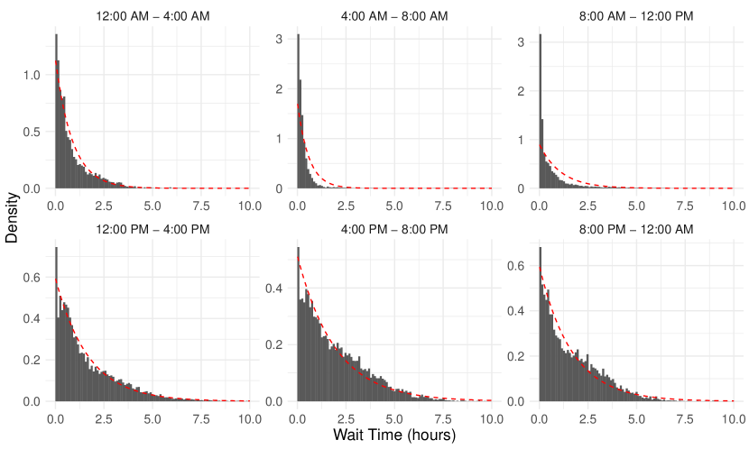
Figure 1: Patient wait time density conditional on time of arrival

Note: The histograms depict the empirical density of patient wait times within each arrival time interval. The red dashed lines are the densities of the fitted exponential distribution conditional on being in each interval. The model we propose will systematically forecast the distributions by conditioning on a richer set of features described in Section 4.

Given this, we test the out-of-sample predictive performance of the classic exponential model where the log-rate parameter $\log\lambda$ is linear in the covariates $x$, i.e. $\lambda=e^{x^{\prime}\beta}$. We fit this model as well as QRF to 2016 data, and then use both models to forecast wait times in the 2017 test period. We repeat the process for the 2018 and 2019 test periods using the preceding year as the training period. As seen in Table 1, the classic exponential model actually results in a CRPS value that is 2.5% lower than that for QRF (lower values are better). In other words, the operations-informed parametric model outperforms the distribution-agnostic ML algorithm in this setting.

Similarly, the histograms for service times are consistent with a log-normal distribution (see Figure 3 the electronic companion). We thus compare the out-of-sample predictive performance of the classic log-normal distribution to the QRF. Specifically, we specify the parameters of the log-normal distribution linearly in $x$, i.e. $\mu_{LN}=x^{\prime}\gamma$ and $\log\sigma_{LN}=x^{\prime}\theta$, and estimate $(\gamma,\theta)$ by maximum likelihood. Once again we find that the classic log-normal model has a CRPS value that is 7.0% lower than that for QRF.

Overall, our results demonstrate that the operations-informed parametric models outperform the nonparametric machine learning QRF in both settings. This underscores the value of operations domain knowledge, demonstrating that it can surpass complex and flexible ML techniques. bGND, which we describe next, is designed to further enhance performance by integrating this knowledge into distributional machine learning.

2.2 Estimation Algorithm for bGND

The approach we propose for estimating bGND (1) is based on the simple observation that there is no need to jointly estimate $\mu(x)$ and $b(x)$, which is what existing approaches do for special cases of bGND such as boosted normal distribution. The location parameter $\mu(x)$, being equal to the conditional mean $\mathbb{E}(Y|x)$ in a GND, can first be estimated using any boosted least-squares regression method that is consistent. We then show that the scale parameter $b(x)$ can be consistently estimated by setting $\mu(x)$ equal to the estimated $\hat{\mu}(x)$. Our approach decouples the estimation into two smooth convex problems even when $\gamma=1$ (i.e. the Laplace distribution), thereby sidestepping the numerical issues faced by existing approaches. Our approach is also more natural as it mirrors how the mean and variance are traditionally estimated.

We first reparameterize the scale parameter as

$$b(x)=e^{-\beta(x)/\gamma}$$ (2)

where $\beta(x)\in\mathbb{R}$. The log-density of (1) then becomes $\beta(x)-|y-\mu(x)|^{\gamma}e^{\beta(x)}$ up to a multiplicative factor. Thus given a sample $\mathcal{S}=\{(x_{i},y_{i})\}_{i=1}^{n}$ of i.i.d. copies of $(X,Y)$ where $Y|X\sim GND(\mu(X),b(X))$, the scaled negative log-likelihood is

$$R_{n}(\mu,\beta,\mathcal{S})=|\mathcal{S}|^{-1}\sum_{i\in\mathcal{S}}\left\{|y_{i}-\mu(x_{i})|^{\gamma}e^{\beta(x_{i})}-\beta(x_{i})\right\}.$$ (3)

We will refer to (3) as the likelihood risk, and its population version is

$$R(\mu,\beta)=\mathbb{E}_{X,Y}R_{n}(\mu,\beta,\{(X,Y)\})=\int\left\{\mathbb{E}_{Y|x}(|Y-\mu(x)|^{\gamma})e^{\beta(x)}-\beta(x)\right\}dP_{X},$$ (4)

where $P_{X}$ is the distribution of $X\in\mathcal{X}\subset\mathbb{R}^{p}$. Its empirical analogue is $P_{X,n_{2}}(B)=n_{2}^{-1}\sum_{i\in\mathcal{S}_{2}}I(x_{i}\in B)$.

Algorithm 1 Fitting the bGND  (1)

1:  Split $\mathcal{S}=\{(x_{i},y_{i})\}_{i=1}^{n}$ into two random subsamples $\mathcal{S}_{1}$ and $\mathcal{S}_{2}$ of equal size, $n_{1}=n_{2}=n/2$

2:  Use any tree-boosted regression method satisfying (5) to estimate $\mu(x)$ from $\mathcal{S}_{1}$. Call this $\hat{\mu}(x)$

3:  Apply a tree-boosted algorithm such as Algorithm 2 in Appendix 6 to minimize the empirical risk $R_{n}(\hat{\mu},\beta,\mathcal{S}_{2})$ over $\mathcal{S}_{2}$. The resulting tree-boosted minimizer is $\hat{\beta}(x)$

4:  The tree-boosted estimators for the location and scale parameters are

$$\hat{\mu}(x),\quad\hat{b}(x)=e^{-\hat{\beta}(x)/\gamma}$$

Algorithm 1 describes our approach for estimating $\mu(x)$ and $\beta(x)$. The analysis of the algorithm is facilitated by sample splitting, an idea from the statistics literature that goes back to at least Bickel (1982). First, we randomly split the sample $\mathcal{S}$ into two disjoint subsamples $\mathcal{S}_{1}$ and $\mathcal{S}_{2}$ of equal size $n_{1}=n_{2}=n/2$. Next, noting that $\mu(x)$ is the conditional mean $\mathbb{E}(Y|x)$, employ any consistent tree-boosted least-squares regression method (for example, Zhang and Yu (2005)) to obtain an estimate $\hat{\mu}(x)$ from $\mathcal{S}_{1}$ that satisfies

$$\|\mu-\hat{\mu}\|_{\infty}=\epsilon_{n_{1}}\rightarrow_{p}0\text{ w.r.t. }\mathcal{S}_{1}.$$ (5)

The final step plugs $\hat{\mu}(x)$ into the empirical risk (3) evaluated on $\mathcal{S}_{2}$, $R_{n}(\hat{\mu},\beta,\mathcal{S}_{2})$, and employs a gradient-boosted algorithm to minimize $R_{n}(\hat{\mu},\beta,\mathcal{S}_{2})$ over $\beta\in\mathcal{F}$, where $\mathcal{F}$ is the span of regression trees characterized in Section 3. Algorithm 2 in Appendix 6 provides one way to do this. The resulting tree-boosted minimizer is our estimate $\hat{\beta}(x)$, and our estimate for the scale parameter is $\hat{b}(x)=e^{-\hat{\beta}(x)/\gamma}$.

3 Statistical Consistency of bGND

In Section 3.1 we show the statistical consistency of our approach, the paper’s main theoretical result. Supporting results can be found in Section 3.2. Our analysis rests on four conditions. The first three are standard for the nonparametric estimation of functions, i.e. $\mu(x)$ and $b(x)$ in our context. The domain of the covariates $\mathcal{X}\subset\mathbb{R}^{p}$ is bounded. The distribution $P_{X}$ of the covariates $X$ admits a density that is bounded away from zero and infinity on $\mathcal{X}$. Define also the empirical distribution $P_{X,n_{2}}(B)=n_{2}^{-1}\sum_{i\in\mathcal{S}_{2}}I(x_{i}\in B)$. The true location parameter $\mu(x)$ is bounded between some interval $[\underline{\mu},\overline{\mu}]\subset(0,\infty)$ on $\mathcal{X}$, and the true scale parameter $b(x)$ is bounded between some interval $[\underline{b},\overline{b}]\subset(0,\infty)$ on $\mathcal{X}$.

To motivate the final assumption, define the span of the regression tree functions that hosts the tree-boosted estimators $\hat{\mu}(x)$ and $\hat{\beta}(x)$ as

$$\mathcal{F}=\left\{\sum_{k=1}^{m}g_{k}(x):m\in\mathbb{N},g_{k}(x)\text{ a regression tree function defined on }\mathcal{X}\right\},$$

and for $\Psi>0$, its restriction

$$\mathcal{F}^{\Psi}=\left\{F\in\mathcal{F}:\|F\|_{\infty}<\Psi\right\}.$$ (6)

In particular, $\mathcal{F}^{\Psi_{n_{2}}}$ contains all the boosting iterates $b_{0},b_{1},\cdots,\hat{b}$ produced by Algorithm 2 in Appendix 6. Following Lee et al. (2021), $\mathcal{F}$ is equivalent to $\{\sum_{j}c_{j}I_{B_{j}}:c_{j}\in\mathbb{R}\}$, i.e. the span of indicator functions over disjoint hypercubes of $\mathcal{X}$ indexed by $j=(j_{1},\cdots,j_{p})$:

$$B_{j}=\left\{\begin{array}[]{ccc}x=(x^{(1)},\cdots,x^{(p)})&:&\begin{array}[]{c}x^{(1,j_{1})}<x^{(1)}\leq x^{(1,j_{1}+1)}\\ \vdots\\ x^{(p,j_{p})}<x^{(p)}\leq x^{(p,j_{p}+1)}\end{array}\end{array}\right\}.$$ (7)

The regions $B_{j}\subset\mathcal{X}$ are formed using all possible split points $\{x^{(k,j_{k})}\}_{j_{k}}$ for the $k$-th coordinate $x^{(k)}$, with the spacing determined by the precision of the measurements. For example, if weight is measured to the closest kilogram, then the set of all possible split points will be $\{0.5,1.5,2.5,\cdots\}$ kilograms. While abstract treatments of trees assume that there is a continuum of split points, in reality they fall on a discrete grid that is pre-determined by the precision of the data.

Given that $x$ is inevitably measured to somewhere within one of these regions, what we can identify from data is not $\mu(x)$ or $b(x)^{\gamma}$, but the coarsened versions

$$\mu^{\ast}(x)\left|{}_{B_{j}}\right. :=\mathbb{E}\{\mu(X)|X\in B_{j}\}=P_{X}(B_{j})^{-1}\int_{B_{j}}\mu(x)dP_{X},$$ (8)

$$\{b^{\ast}(x)\}^{\gamma}\left|{}_{B_{j}}\right. :=\mathbb{E}\{b(X)^{\gamma}|X\in B_{j}\}=P_{X}(B_{j})^{-1}\int_{B_{j}}b(x)^{\gamma}dP_{X},$$

i.e. the true $\mu(x)$ and $b(x)$ are identified up to a piecewise-constant approximation within each fundamental partition $B_{j}$, i.e. $\mu^{\ast},b^{\ast}\in\mathcal{F}$. Recall that this is a measurement precision issue, so it holds regardless of the algorithm we use to estimate the parameters. The approximation errors $\|\mu-\mu^{\ast}\|_{\infty}$ and $\|b-b^{\ast}\|_{\infty}$ are thus irreducible, and we consider them to be negligible in a numerical tolerance sense. $\|\mu-\mu^{\ast}\|_{\infty}=\|b-b^{\ast}\|_{\infty}=0$.

Remark 3.1

If $\mu(x)$ and $b(x)$ are sufficiently smooth, $\mu^{\ast}(x)$ and $b^{\ast}(x)$ will closely approximate them within a small enough partition $B_{j}$ even without Assumption 3. To see this, suppose that $b(x)$ is Hölder continuous, i.e. $|b(x)-b(x^{\prime})|\precsim\|x-x^{\prime}\|^{\alpha}$ for some $\alpha>0$. Then $\inf_{x\in B_{j}}b(x)\leq b^{\ast}(x)|_{B_{j}}\leq\sup_{x\in B_{j}}b(x)$ and

$$\left\|b-b^{\ast}\right\|_{\infty}\precsim\max_{j}(\text{diam}B_{j})^{\alpha}.$$

A similar result holds for $\left\|\mu-\mu^{\ast}\right\|_{\infty}$. When the covariates are measured to high precision, the diameter of the $B_{j}$’s will be small, which implies close uniform approximation of $b$ by $b^{\ast}$ and of $\mu$ by $\mu^{\ast}$.

Remark 3.2

Assumption 3 implies the following, which will be useful in various parts of the proof:

$$\rho_{X}=\min_{j}P_{X}(B_{j})>0.$$

Remark 3.3

Since $\mathcal{F}$ is the linear span of piecewise-constant functions, it is closed under pointwise exponentiation, i.e. $f\in\mathcal{F}\Rightarrow e^{f}\in\mathcal{F}$. Likewise, $f\in\mathcal{F}\Rightarrow f^{1/\gamma}\in\mathcal{F}$. Hence $\mu^{\ast},b^{\ast},\hat{b}\in\mathcal{F}$.

3.1 Consistency of $(\hat{\mu},\hat{b})$

We are now in a position to state our main result. For $Y|x\sim bGND(\mu(x),b(x))$, $\hat{\mu}$ is by default a consistent estimator for $\mu$ due to (5), so it remains to show that the estimator $\hat{b}$ for the scale is also consistent. Proposition 3.4 below can also be expressed in non-asymptotic terms but we omit the analysis for brevity.

Proposition 3.4

Under Assumptions 3-3,

$$\|\hat{b}-b\|_{\infty}=o_{p}(1).$$

To establish the result, we first show that the minimizer $\beta^{\ast}_{\hat{\mu}}(x)=\arg\min_{\beta(x)\in\mathcal{F}}R(\hat{\mu},\beta)$ exists, and denote $b^{\ast}_{\hat{\mu}}(x)=e^{-\beta^{\ast}_{\hat{\mu}}(x)/\gamma}$. Given that $\mathcal{F}$ is the span of piecewise-constant functions over the fundamental partitions $\{B_{j}\}_{j}$ in (7), we can write $\hat{\mu}(x)=\sum_{j}\hat{\mu}|_{B_{j}}I_{B_{j}}(x)$, $\beta^{\ast}_{\hat{\mu}}(x)=\sum_{j}\beta^{\ast}_{\hat{\mu}}|_{B_{j}}I_{B_{j}}(x)$, and $b^{\ast}_{\hat{\mu}}(x)=\sum_{j}e^{-\beta^{\ast}_{\hat{\mu}}|_{B_{j}}/\gamma}I_{B_{j}}(x)$.

Lemma 3.5

If $\|\mu-\hat{\mu}\|_{\infty}=\epsilon_{n_{1}}<\infty$ in (5) then $\beta^{\ast}_{\hat{\mu}}$ exists and its value inside $B_{j}$ satisfies

$$b^{\ast}_{\hat{\mu}}(x)^{\gamma}|_{B_{j}}=e^{-\beta^{\ast}_{\hat{\mu}}|_{B_{j}}}=P_{X}(B_{j})^{-1}\int_{B_{j}}\mathbb{E}_{Y|x}\left|Y-\hat{\mu}|_{B_{j}}\right|^{\gamma}dP_{X}=\mathbb{E}(\left|Y-\hat{\mu}|_{B_{j}}\right|^{\gamma}|X\in B_{j}).$$

Furthermore $\|b^{\ast}_{\hat{\mu}}-b\|_{\infty}<\epsilon_{n_{1}}$, and lastly, if $\epsilon_{n_{1}}\leq\underline{b}/2$ then

$$\underline{b}/2\leq b^{\ast}_{\hat{\mu}}(x)\leq 2\overline{b}\text{ and }-\gamma\log(2\overline{b})\leq\beta^{\ast}_{\hat{\mu}}(x)\leq\gamma\log(2/\underline{b}).$$

Proof 3.6

Proof. Since $\|\hat{\mu}\|_{\infty}\leq\epsilon_{n_{1}}+\|\mu\|_{\infty}<\infty$,

$$R(\hat{\mu},\beta) =\mathbb{E}_{X,Y}R_{n}(\hat{\mu},\beta,\{(X,Y)\})=\sum_{j}\int_{B_{j}}\left\{\mathbb{E}_{Y|x}\left|Y-\hat{\mu}|_{B_{j}}\right|^{\gamma}e^{\beta|_{B_{j}}}-\beta|_{B_{j}}\right\}dP_{X}$$

$$=\sum_{j}\left\{e^{\beta|_{B_{j}}}\int_{B_{j}}\mathbb{E}_{Y|x}\left|Y-\hat{\mu}|_{B_{j}}\right|^{\gamma}dP_{X}-\beta|_{B_{j}}P_{X}(B_{j})\right\}.$$

By Remark 3.2, $P_{X}(B_{j})>0\,\,\forall j$ so the first order condition for each $\beta|_{B_{j}}$ implies the first claim. For the second claim,

$$b^{\ast}_{\hat{\mu}}\left|{}_{B_{j}}\right.=e^{-\beta^{\ast}_{\hat{\mu}}|_{B_{j}}/\gamma} =\left(\int_{B_{j}}\mathbb{E}_{Y|x}\left|Y-\hat{\mu}|_{B_{j}}\right|^{\gamma}d\frac{P_{X}}{P_{X}(B_{j})}\right)^{1/\gamma}=\left\|Y-\hat{\mu}\right\|_{B_{j},\gamma}$$

$$\leq\left\|Y-\mu\right\|_{B_{j},\gamma}+\left\|\mu-\hat{\mu}\right\|_{B_{j},\gamma}\leq\left\|Y-\mu\right\|_{B_{j},\gamma}+\epsilon_{n_{1}}=b^{\ast}|_{B_{j}}+\epsilon_{n_{1}},$$

where the last equality comes from noting that $\mathbb{E}_{Y|x}\left|Y-\mu(x)\right|^{\gamma}=b(x)^{\gamma}$ and from the definition of $b^{\ast}(x)$ in (8). Reversing the roles of $b^{\ast}_{\hat{\mu}}$ and $b^{\ast}$ shows that $\|b^{\ast}_{\hat{\mu}}-b\|_{\infty}\leq\|b^{\ast}_{\hat{\mu}}-b^{\ast}\|_{\infty}+\|b^{\ast}-b\|_{\infty}<\epsilon_{n_{1}}$ by Assumption 3. For the final claim, note from (8) that $\underline{b}\leq b^{\ast}(x)\leq\overline{b}$. Since $\|b^{\ast}_{\hat{\mu}}-b^{\ast}\|_{\infty}\leq\epsilon_{n_{1}}$ and $\epsilon_{n_{1}}\leq\underline{b}/2$ by hypothesis,

$$\underline{b}/2=\underline{b}-\underline{b}/2\leq b^{\ast}(x)-\epsilon_{n_{1}}\leq b^{\ast}_{\hat{\mu}}(x)\leq b^{\ast}(x)+\epsilon_{n_{1}}\leq\overline{b}+\overline{b}=2\overline{b},$$

and the bound for $\beta^{\ast}_{\hat{\mu}}$ follows immediately from $b^{\ast}_{\hat{\mu}}(x)=e^{-\beta^{\ast}_{\hat{\mu}}/\gamma}$.

Proof 3.7

Proof of Proposition 3.4.

From (5) and Lemma 3.5 we have $\|\hat{b}-b\|_{\infty}\leq\|\hat{b}-b^{\ast}_{\hat{\mu}}\|_{\infty}+\epsilon_{n_{1}}$ where $\epsilon_{n_{1}}=o_{p}(1)$ w.r.t. the sample $\mathcal{S}_{1}$, so eventually $\epsilon_{n_{1}}\leq\underline{b}/2$ with high probability, thus satisfying the hypothesis in Lemma 3.5. It then suffices to show that $\|\hat{b}-b^{\ast}_{\hat{\mu}}\|_{\infty}=o_{p}(1)$ w.r.t. the sample $\mathcal{S}_{2}$. By virtue of $\beta^{\ast}_{\hat{\mu}}$ being the minimizer of the population risk $R(\hat{\mu},\beta)$ in (4), there exists $\rho\in(0,1)$ for which Taylor’s theorem yields the first equality below:

$$0 \leq R(\hat{\mu},\hat{\beta})-R(\hat{\mu},\beta^{\ast}_{\hat{\mu}})=\frac{1}{2}\int\mathbb{E}_{Y|x}\{|Y-\hat{\mu}(x)|^{\gamma}\}e^{\beta^{\ast}_{\hat{\mu}}(x)+\rho\{\hat{\beta}(x)-\beta^{\ast}_{\hat{\mu}}(x)\}}\cdot\{\hat{\beta}(x)-\beta^{\ast}_{\hat{\mu}}(x)\}^{2}dP_{X}$$

$$=\frac{1}{2}\sum_{j}e^{\rho(\hat{\beta}|_{B_{j}}-\beta^{\ast}_{\hat{\mu}}|_{B_{j}})}\cdot(\hat{\beta}|_{B_{j}}-\beta^{\ast}_{\hat{\mu}}|_{B_{j}})^{2}P_{X}(B_{j})\geq\frac{1}{2}e^{-\|\hat{\beta}-\beta^{\ast}_{\hat{\mu}}\|_{\infty}}\rho_{X}\|\hat{\beta}-\beta^{\ast}_{\hat{\mu}}\|_{\infty}^{2},$$

where the second equality follows from noting that all terms apart from $\mathbb{E}_{Y|x}\{|Y-\hat{\mu}(x)|^{\gamma}\}$ is constant within each region $B_{j}$, and that $\int_{B_{j}}\mathbb{E}_{Y|x}\left|Y-\hat{\mu}|_{B_{j}}\right|^{\gamma}dP_{X}=e^{-\beta^{\ast}_{\hat{\mu}}|_{B_{j}}}P_{X}(B_{j})$ from Lemma 3.5. Suppressing the notation $\mathcal{S}_{2}$ in $R_{n}(\hat{\mu},\beta,\mathcal{S}_{2})$, it follows from the inequality $|e^{u}-e^{v}|\leq\max(e^{u},e^{v})|u-v|$ that

$$\|\hat{b}-b^{\ast}_{\hat{\mu}}\|_{\infty} \leq\max_{x\in\mathcal{X}}\{\hat{b}(x)\vee b^{\ast}_{\hat{\mu}}(x)\}\|\hat{\beta}-\beta^{\ast}_{\hat{\mu}}\|_{\infty}/\gamma\leq\underbrace{\frac{\max_{x\in\mathcal{X}}\{\hat{b}(x)\vee b^{\ast}_{\hat{\mu}}\}e^{\frac{1}{2}\|\hat{\beta}-\beta^{\ast}_{\hat{\mu}}\|_{\infty}}}{\gamma(\rho_{X}/2)^{1/2}}}_{C}\{R(\hat{\mu},\hat{\beta})-R(\hat{\mu},\beta^{\ast}_{\hat{\mu}})\}^{1/2}$$ (9)

$$\leq C\{\underbrace{R(\hat{\mu},\hat{\beta})-R_{n}(\hat{\mu},\hat{\beta})}_{(i)}+\underbrace{R_{n}(\hat{\mu},\hat{\beta})-R_{n}(\hat{\mu},\beta^{\ast}_{\hat{\mu}})}_{(ii)}+\underbrace{R_{n}(\hat{\mu},\beta^{\ast}_{\hat{\mu}})-R(\hat{\mu},\beta^{\ast}_{\hat{\mu}})}_{(iii)}\}^{1/2}.$$

The fraction $C$ is bounded with high probability w.r.t. the sample $\mathcal{S}_{2}$ because $\min_{j}P_{X}(B_{j})>0$ by Remark 3.2, $\{b^{\ast}_{\hat{\mu}}(x),\beta^{\ast}_{\hat{\mu}}(x)\}$ are bounded by Lemma 3.5, and $\{\hat{\beta}(x),\hat{b}(x)\}$ are bounded with high probability by Lemma 3.18. The quantities (i) and (iii) are the deviations of the empirical risk from the population risk. Proposition 3.8 in Section 3.2.1 develops concentration inequalities to show that both quantities are $o_{p}(1)$ w.r.t. $\mathcal{S}_{2}$, bearing in mind that $\hat{\beta}\in\mathcal{F}^{\Psi_{n_{2}}}$ (6). Finally, (ii) represents the minimization of the empirical risk (3). Proposition 3.20 in Section 3.2.2 shows that this term is also $o_{p}(1)$ w.r.t. $\mathcal{S}_{2}$.

3.2 Supporting results

From now on we will suppress the notation $\mathcal{S}_{2}$ from the empirical risk $R_{n}(\hat{\mu},\beta,\mathcal{S}_{2})$. Let us also recall basic concepts for empirical processes from Chapter 2 of van der Vaart and Wellner (1996) that will be used in $\S$3.2.1. For a probability measure $P$ on $\mathcal{X}$, the $L^{2}(P)$-ball of radius $\delta>0$ centred at some $\beta\in L^{2}(P)$ is $\{\beta^{\prime}\in\mathcal{F}^{\Psi}:\int(\beta^{\prime}-\beta)^{2}dP<\delta^{2}\}$ where $\mathcal{F}^{\Psi}$ is defined in (6). The covering number $\mathcal{N}(\delta,\mathcal{F}^{\Psi},P)$ is the minimum number of such balls needed to cover $\mathcal{F}^{\Psi}$, so $\mathcal{N}(\delta,\mathcal{F}^{\Psi},P)=1$ for $\delta\geq\Psi$. The entropy integral

$$J_{\mathcal{F}}=\sup_{\Psi>0,P}\int_{0}^{1}\sqrt{\log\mathcal{N}(u\Psi,\mathcal{F}^{\Psi},P)}du$$ (10)

represents the complexity of the function class $\mathcal{F}$, and is at most finite because $\mathcal{F}$ is the span of indicator functions over a finite number of regions (7). For convenience we will assume that $J_{\mathcal{F}}>1$.

3.2.1 Concentration inequalities.

The results herein are greatly facilitated by decomposing $(X,Y)$ into independent components $X$ and $W$: Let $\{W_{i}\}_{i\in\mathcal{S}_{2}}$ be i.i.d. $GND(0,1)$ random variables that are independent of $\{X_{i},Y_{i}\}_{i\in\mathcal{S}_{2}}$. Then conditional on $X_{i}$, $Y_{i}^{\prime}=\mu(X_{i})+b(X_{i})W_{i}$ has the same distribution as $Y_{i}|X_{i}$. Thus the empirical risk $R_{n}(\hat{\mu},\beta)$ has the same distribution as

$$R_{n}^{\prime}(\hat{\mu},\beta)=n_{2}^{-1}\sum_{i\in\mathcal{S}_{2}}\left\{|Y_{i}^{\prime}-\hat{\mu}(X_{i})|^{\gamma}e^{\beta(X_{i})}-\beta(X_{i})\right\}.$$ (11)

The decomposition allows us to condition on the set $\mathcal{W}=\{|W_{1}|,\cdots,|W_{n_{2}}|\leq 2\gamma\log n_{2}\}$, on which

$$\max_{i\in\mathcal{S}_{2}}|Y^{\prime}_{i}-\hat{\mu}(X_{i})|\leq\overline{b}\max_{i\in\mathcal{S}_{2}}|W_{i}|+\epsilon_{n_{1}}<3\gamma\overline{b}\log n_{2}$$ (12)

when $\|\mu-\hat{\mu}\|_{\infty}=\epsilon_{n_{1}}$ in (5) is less than $\underline{b}/2$ eventually. Writing $Q_{n_{2}}=P(|W|>2\gamma\log n_{2})$, the conditional expectation of an integrable $f$ on $\mathcal{X}^{n_{2}}\times\mathcal{W}$ can be re-expressed as an unconditional one:

$$\mathbb{E}\{f(X,W)|\mathcal{W}\} =\mathbb{E}_{X_{1},\cdots,X_{n_{2}}}\int_{|W_{1}|,\cdots,|W_{n_{2}}|\leq 2\gamma\log n_{2}}f\cdot\prod_{i\in\mathcal{S}_{2}}\frac{dP_{W_{i}}}{1-Q_{n_{2}}}$$ (13)

$$=\mathbb{E}_{X_{1},\cdots,X_{n_{2}}}\int f\cdot\prod_{i\in\mathcal{S}_{2}}dP_{Z_{i}}=\mathbb{E}f(X,Z)$$

where the i.i.d. $\{Z_{i}\}_{i\in\mathcal{S}_{2}}$ are each bounded between $\pm 2\gamma\log n_{2}$, and are independent of $\{X_{i},Y_{i}\}_{i\in\mathcal{S}_{2}}$.

Proposition 3.8

Recall that $P_{X,n_{2}}$ is the empirical measure defined in Assumption 3, and $\mathcal{F}^{\Psi}$ is defined in (6). For $n_{2}\geq 3$ and $\|\mu-\hat{\mu}\|_{\infty}=\epsilon_{n_{1}}\leq\underline{b}/2$ in (5), there exist constants $\kappa_{1},\kappa_{2}$ depending on $\gamma$, $\underline{b}$, and $\overline{b}$ such that with probability $1-\kappa_{1}\exp\left\{-\kappa_{2}(\eta\wedge\rho_{X}/J_{\mathcal{F}})^{2}n_{2}^{2/5}\right\}-\gamma n_{2}^{-1}$, we have for $\eta\leq 1$:

$$\min_{j}P_{X,n_{2}}(B_{j})\geq\rho_{X}/2,\qquad\sup_{\beta\in\mathcal{F}^{\Psi_{n_{2}}}}\big{|}R_{n}(\hat{\mu},\beta)-R(\hat{\mu},\beta)\big{|}\leq 2\eta,\qquad\big{|}R_{n}(\hat{\mu},\beta^{\ast}_{\hat{\mu}})-R(\hat{\mu},\beta^{\ast}_{\hat{\mu}})\big{|}\leq\eta,$$

$$\big{|}R_{n}(\hat{\mu},0)-R(\hat{\mu},0)\big{|}=\left|n_{2}^{-1}\sum_{i\in\mathcal{S}_{2}}|Y_{i}-\hat{\mu}(X_{i})|^{\gamma}-\mathbb{E}|Y_{i}-\hat{\mu}(X_{i})|^{\gamma}\right|\leq\eta.$$

Proof 3.9

Proof. Note that $|Y^{\prime}_{i}-\hat{\mu}(X_{i})|^{\gamma}$ has a subexponential tail (consider for example the square of the normal distribution, i.e. chi-squared distribution). We therefore truncate it to facilitate a maximal inequality for the deviation of $R_{n}^{\prime}(\hat{\mu},\beta)$ in (11) from $R(\hat{\mu},\beta)$ based on subgaussian increments: By the hypotheses in the proposition, $\max_{i\in\mathcal{S}_{2}}|Y^{\prime}_{i}-\hat{\mu}(X_{i})|^{\gamma}$ is bounded on $\mathcal{W}$ per (12). Denoting the events

$$U_{\mathcal{F}^{\Psi_{n_{2}}}}=\left\{\sup_{\beta\in\mathcal{F}^{\Psi_{n_{2}}}}\big{|}\{R_{n}^{\prime}(\hat{\mu},\beta)-R_{n}^{\prime}(\hat{\mu},0)\}-\{R(\hat{\mu},\beta)-R(\hat{\mu},0)\}\big{|}>\eta\right\},$$

$$U_{0}=\left\{\big{|}R_{n}^{\prime}(\hat{\mu},0)-R(\hat{\mu},0)\big{|}>\eta\right\},\qquad U_{\beta^{\ast}_{\hat{\mu}}}=\left\{\big{|}R_{n}^{\prime}(\hat{\mu},\beta^{\ast}_{\hat{\mu}})-R(\hat{\mu},\beta^{\ast}_{\hat{\mu}})\big{|}>\eta\right\},$$

we seek a bound for

$$P\left(U_{\mathcal{F}^{\Psi_{n_{2}}}}\cup U_{0}\cup U_{\beta^{\ast}_{\hat{\mu}}}\right) \leq P\left(U_{\mathcal{F}^{\Psi_{n_{2}}}}\cup U_{0}\cup U_{\beta^{\ast}_{\hat{\mu}}},\mathcal{W}\right)+P(\mathcal{W}^{c})\leq P\left(\left.U_{\mathcal{F}^{\Psi_{n_{2}}}}\cup U_{0}\cup U_{\beta^{\ast}_{\hat{\mu}}}\right|\mathcal{W}\right)+\gamma n_{2}^{-1}$$ (14)

$$\leq P\left(\left.U_{\mathcal{F}^{\Psi_{n_{2}}}}\right|\mathcal{W}\right)+P\left(\left.U_{0}\right|\mathcal{W}\right)+P\left(\left.U_{\beta^{\ast}_{\hat{\mu}}}\right|\mathcal{W}\right)+\gamma n_{2}^{-1},$$

where the second inequality comes from Lemma 3.14 and the fact that $P(A\cap B)\leq P(A|B)$. An issue with bounding these probabilities is that, by conditioning on $\mathcal{W}$, $R_{n}^{\prime}(\hat{\mu},\beta)$ concentrates around $\mathbb{E}\{R_{n}^{\prime}(\hat{\mu},\beta)|\mathcal{W}\}$ rather than $R(\hat{\mu},\beta)$. Thus define instead

$$V_{\beta}=\{R_{n}^{\prime}(\hat{\mu},\beta)-R_{n}^{\prime}(\hat{\mu},0)\}-[\mathbb{E}\{R_{n}^{\prime}(\hat{\mu},\beta)|\mathcal{W}\}-\mathbb{E}\{R_{n}^{\prime}(\hat{\mu},0)|\mathcal{W}\}],$$

$$V_{0}=R_{n}^{\prime}(\hat{\mu},0)-\mathbb{E}\{R_{n}^{\prime}(\hat{\mu},0)|\mathcal{W}\},\qquad V_{\beta^{\ast}_{\hat{\mu}}}=R_{n}^{\prime}(\hat{\mu},\beta^{\ast}_{\hat{\mu}})-\mathbb{E}\{R_{n}^{\prime}(\hat{\mu},\beta^{\ast}_{\hat{\mu}})|\mathcal{W}\}.$$

Lemma 3.16 shows that the probabilities in (14) can be bounded in terms of the $V$’s. This is used in Lemmas 3.10 and 3.12, which collectively imply

$$P\left(U_{\mathcal{F}^{\Psi_{n_{2}}}}\cup U_{0}\cup U_{\beta^{\ast}_{\hat{\mu}}}\right)\leq\kappa_{3}\exp\left\{-\kappa_{4}(\eta/J_{\mathcal{F}})^{2}n_{2}^{2/5}\right\}+2\kappa_{5}\exp\left(-\kappa_{6}\eta^{2}n_{2}^{1/2}\right)+\gamma n_{2}^{-1}$$

$$\qquad\leq(\kappa_{3}+2\kappa_{5})\exp\left\{-(\kappa_{4}\wedge\kappa_{6})(\eta/J_{\mathcal{F}})^{2}n_{2}^{2/5}\right\}+\gamma n_{2}^{-1}=\kappa_{1}\exp\left\{-\kappa_{2}(\eta/J_{\mathcal{F}})^{2}n_{2}^{2/5}\right\}+\gamma n_{2}^{-1},$$

where the second inequality follows from assuming that $J_{\mathcal{F}}>1$ in (10). Note from Lemma 3.10 that $\min_{j}P_{X,n_{2}}(B_{j})\geq\rho_{X}/2$ with probability $1-\kappa_{3}\exp\{-\kappa_{4}(\rho_{X}/J_{\mathcal{F}})^{2}n_{2}\}$, so by enlarging $\kappa_{1}$ we have both events $\left\{\min_{j}P_{X,n_{2}}(B_{j})\geq\rho_{X}/2\right\}$ and $\left\{U_{\mathcal{F}^{\Psi_{n_{2}}}}^{C}\cap U_{0}^{C}\cap U_{\beta^{\ast}_{\hat{\mu}}}^{C}\right\}$ hold with probability $1-\kappa_{1}\exp\left\{-\kappa_{2}(\eta\wedge\rho_{X}/J_{\mathcal{F}})^{2}n_{2}^{2/5}\right\}-\gamma n_{2}^{-1}$. Finally, noting that $\big{|}R_{n}(\hat{\mu},\beta)-R(\hat{\mu},\beta)\big{|}\leq 2\eta$ on $U_{\mathcal{F}^{\Psi_{n_{2}}}}^{C}\cap U_{0}^{C}$ concludes the proof.

Lemma 3.10

There exist constants $\kappa_{3}$, $\kappa_{4}$ depending on $\gamma$, $\underline{b}$, and $\overline{b}$ for which $\min_{j}P_{X,n_{2}}(B_{j})\geq\rho_{X}/2$ with probability $1-\kappa_{3}\exp\{-\kappa_{4}(\rho_{X}/J_{\mathcal{F}})^{2}n_{2}\}$, and

$$P\left(\left.U_{{\mathcal{F}^{\Psi_{n_{2}}}}}\right|\mathcal{W}\right)\leq\kappa_{3}\exp\left\{-\kappa_{4}(\eta/J_{\mathcal{F}})^{2}n_{2}^{2/5}\right\}.$$

Proof 3.11

Proof. From Lemma 3.16 we have $P\left(\left.U_{{\mathcal{F}^{\Psi_{n_{2}}}}}\right|\mathcal{W}\right)\leq P(\sup_{\beta\in\mathcal{F}^{\Psi_{n_{2}}}}|V_{\beta}|>\eta-\tau_{1}/n_{2}^{3/2}|\mathcal{W})$. To bound this, define the Orlicz norm $\|X\|_{\Phi}=\inf\{C>0:\mathbb{E}\Phi(|X|/C)\leq 1\}$ where $\Phi(x)=e^{x^{2}}-1$. Taking expectations w.r.t. $(X,Z)$ in (13), suppose the following bounds hold for some constant $\tau_{2}$ depending on $\gamma$, $\underline{b}$, and $\overline{b}$:

$$\left\|\sup_{\beta\in\mathcal{F}^{\Psi_{n_{2}}}}|V_{\beta}|\right\|_{\Phi}\leq\tau_{2}J_{\mathcal{F}}/n_{2}^{1/5},\qquad\left\|\sup_{\beta\in\mathcal{F}^{1}}\left|n_{2}^{-1}\sum_{i\in\mathcal{S}_{2}}\beta(X_{i})-\mathbb{E}_{X}\beta(X)\right|\right\|_{\Phi}\leq\tau_{2}J_{\mathcal{F}}/n_{2}^{1/2}.$$ (15)

Applying Markov’s inequality to the first inequality in (15) implies that for $\eta>\tau_{1}/n_{2}^{3/2}$,

$$\quad P\left(\left.\sup_{\beta\in\mathcal{F}^{\Psi_{n_{2}}}}|V_{\beta}|>\eta-\tau_{1}/n_{2}^{3/2}\right|\mathcal{W}\right)$$

$$\leq 2\exp\left\{-\left(\frac{\eta-\tau_{1}/n_{2}^{3/2}}{\tau_{2}J_{\mathcal{F}}}\right)^{2}n_{2}^{2/5}\right\}\leq 2\exp\left\{\frac{2\tau_{1}\eta}{(\tau_{2}J_{\mathcal{F}})^{2}n_{2}^{11/10}}-\left(\frac{\eta}{\tau_{2}J_{\mathcal{F}}}\right)^{2}n_{2}^{2/5}\right\}$$

$$\leq 2\exp\left\{\frac{2\tau_{1}}{\tau_{2}^{2}3^{11/10}}-\tau_{2}^{\prime}(\eta/J_{\mathcal{F}})^{2}n_{2}^{2/5}\right\}=\kappa_{3}\exp\left\{-\kappa_{4}(\eta/J_{\mathcal{F}})^{2}n_{2}^{2/5}\right\},$$

recalling that $J_{\mathcal{F}}>1$ in the last inequality. Noting that the indicators $I_{B_{j}}(\cdot)$ over the regions (7) belong in $\mathcal{F}^{1}$, $\max_{j}|P_{X,n_{2}}(B_{j})-P_{X}(B_{j})|\leq\rho_{X}/2\Rightarrow\min_{j}P_{X,n_{2}}(B_{j})\geq\rho_{X}/2$ with probability $1-2\exp\{-(\kappa_{4}/4)(\rho_{X}/J_{\mathcal{F}})^{2}n_{2}\}$ under the second inequality in (15). Hence adjust the definitions of $\kappa_{3},\kappa_{4}$.

Thus it remains to show (15). For the first inequality, let $\{\zeta_{i}\}_{i}$ be independent Rademacher random variables that are independent of $\{X_{i},Z_{i}\}_{i\in\mathcal{S}_{2}}$. It follows from the symmetrization Lemma 2.3.1 of van der Vaart and Wellner (1996) that $\left\|\sup_{\beta\in\mathcal{F}^{\Psi_{n_{2}}}}|V_{\beta}|\right\|_{\Phi}$ is bounded by

$$2\left\|n_{2}^{-1}\sup_{\beta\in\mathcal{F}^{\Psi_{n_{2}}}}|\sum_{i\in\mathcal{S}_{2}}\zeta_{i}\{l_{i}(F)-l_{i}(0)\}|\right\|_{\Phi}$$

$$\leq \frac{2}{n_{2}}\left\|\sup_{\beta\in\mathcal{F}^{\Psi_{n_{2}}}}|\sum_{i\in\mathcal{S}_{2}}\zeta_{i}|Y_{i}^{\prime}-\hat{\mu}(X_{i})|^{\gamma}\left\{e^{\beta(X_{i})}-e^{0}\right\}|\right\|_{\Phi}+\frac{2}{n_{2}}\left\|\sup_{\beta\in\mathcal{F}^{\Psi_{n_{2}}}}|\sum_{i\in\mathcal{S}_{2}}\zeta_{i}\beta(X_{i})|\right\|_{\Phi}$$

$$\leq \frac{2}{n_{2}}\Big{\{}2(3\gamma\overline{b}\log n_{2})^{\gamma}e^{\Psi_{n_{2}}}+1\Big{\}}\left\|\sup_{\beta\in\mathcal{F}^{\Psi_{n_{2}}}}|\sum_{i\in\mathcal{S}_{2}}\zeta_{i}\beta(X_{i})|\right\|_{\Phi}\leq\tau_{2}\frac{e^{\Psi_{n_{2}}}(\log n_{2})^{\gamma}}{n_{2}}\left\|\sup_{\beta\in\mathcal{F}^{\Psi_{n_{2}}}}\sum_{i\in\mathcal{S}_{2}}\zeta_{i}\beta(X_{i})\right\|_{\Phi},$$

where the first term inside the curly brackets in the second inequality comes Theorem 4.12 of Ledoux and Talagrand (1991): The map $\beta\mapsto\{(3\gamma\overline{b}\log n_{2})^{\gamma}e^{\Psi_{n_{2}}}\}^{-1}|Y_{i}^{\prime}-\hat{\mu}(X_{i})|^{\gamma}(e^{\beta}-e^{0})$ is a contraction for $|\beta|<\Psi_{n_{2}}$ because $|e^{x}-e^{y}|\leq e^{\max(x,y)}|x-y|$ and because of (12). We drop the absolute value inside the supremum because $\mathcal{F}^{\Psi_{n_{2}}}$ is closed under negation. Now hold $\{X_{i},Z_{i}\}_{i\in\mathcal{S}_{2}}$ fixed so that only $\{\zeta_{i}\}_{i}$ is stochastic. By Corollary 2.2.7 and Theorem 2.2.4 of van der Vaart and Wellner (1996),

$$\left\|\sup_{\beta\in\mathcal{F}^{\Psi_{n_{2}}}}|V_{\beta}|\right\|_{\Phi} \leq\tau_{2}^{\prime}\frac{e^{\Psi_{n_{2}}}(\log n_{2})^{\gamma}}{n_{2}^{1/2}}\int_{0}^{\Psi_{n_{2}}}\sqrt{\log\mathcal{N}(u,\mathcal{F}^{\Psi_{n_{2}}},P_{n_{2}})}du\leq\tau_{2}^{\prime}\frac{\Psi_{n_{2}}e^{\Psi_{n_{2}}}(\log n_{2})^{\gamma}}{n_{2}^{1/2}}J_{\mathcal{F}}$$

$$=\tau_{2}^{\prime}\frac{(\log n_{2})^{\gamma}}{n_{2}^{1/10}}\cdot\frac{\Psi_{n_{2}}e^{\Psi_{n_{2}}}}{n_{2}^{1/5}}J_{\mathcal{F}}/n_{2}^{1/5}=\tau_{2}^{\prime\prime}J_{\mathcal{F}}/n_{2}^{1/5},$$

where the second inequality follows from (10), and the last equality from $\Psi_{n_{2}}e^{\Psi_{n_{2}}}=n_{2}^{1/5}$ in Algorithm 2 and from the fact that $(\log n_{2})^{\gamma}/n^{1/10}\leq(10\gamma/e)^{\gamma}$ for $n_{2}\geq 2$. The bound does not depend on $\{X_{i},Z_{i}\}_{i\in\mathcal{S}_{2}}$, so the first inequality in (15) holds. The second inequality in (15) follows the same approach.

Lemma 3.12

For $\beta\in\{0,\beta^{\ast}_{\hat{\mu}}\}$, there exist positive constants $\kappa_{5},\kappa_{6}$ depending on $\gamma$, $\underline{b}$, and $\overline{b}$ for which

$$P\left(|R_{n}^{\prime}(\hat{\mu},\beta)-R(\hat{\mu},\beta)|>\eta|\mathcal{W}\right)\leq\kappa_{5}\exp\left(-\kappa_{6}\eta^{2}n_{2}^{1/2}\right).$$

Proof 3.13

Proof. Conditioning on $\mathcal{W}$, by (12) we have

$$-\|\beta\|_{\infty}\leq l(\beta)=|Y^{\prime}-\hat{\mu}(X)|^{\gamma}e^{\beta(X)}-\beta(X)\leq e^{\|\beta\|_{\infty}}(3\gamma\overline{b}\log n_{2})^{\gamma}+\|\beta\|_{\infty},$$

from which it follows that the image of $l(\beta)$ is bounded by an interval no wider than $3e^{\|\beta\|_{\infty}}(3\gamma\overline{b}\log n_{2})^{\gamma}$. Noting that $(\log n_{2})^{\gamma}/n^{1/4}\leq(4\gamma/e)^{\gamma}$ for $n_{2}\geq 2$, we can further bound the interval width by $\tau_{4}n_{2}^{1/4}$. Using Lemma 3.16 and Hoeffding’s inequality shows that for $\eta>\tau_{3}/n_{2}^{7/4}$,

$$P\left(|R_{n}^{\prime}(\hat{\mu},\beta)-R(\hat{\mu},\beta)|>\eta|\mathcal{W}\right) \leq P\left(\left.\left|R_{n}^{\prime}(\hat{\mu},\beta)-\mathbb{E}(R_{n}^{\prime}(\hat{\mu},\beta)|\mathcal{W})\right|>\eta-\tau_{3}/n_{2}^{7/4}\right|\mathcal{W}\right)$$

$$\leq 2\exp\left\{-2n_{2}\left(\frac{\eta-\tau_{3}/n_{2}^{7/4}}{\tau_{4}n_{2}^{1/4}}\right)^{2}\right\}\leq 2\exp\left(\frac{(4\tau_{3}/\tau_{4}^{2})\eta}{n_{2}^{5/4}}-2\eta^{2}/\tau_{4}^{2}n_{2}^{1/2}\right)$$

$$\leq 2\exp\left\{\frac{(4\tau_{3}/\tau_{4}^{2})}{3^{5/4}}-\tau_{4}^{\prime}\eta^{2}n_{2}^{1/2}\right\}\leq\tau_{3}^{\prime\prime\prime}\exp\left(-\tau_{4}^{\prime}\eta^{2}n_{2}^{1/2}\right).$$

Lemma 3.14

For $W_{1},\cdots,W_{n_{2}}$ independent draws from $GND(0,1)$,

$$P\left\{\max_{i=1,\cdots,n_{2}}|W_{i}|>2\gamma\log n_{2}\right\}<\gamma n_{2}^{-1},\quad\mathbb{E}\{|W|^{\gamma}I_{(|W|>2\gamma\log n_{2})}\}\leq\frac{6\log n_{2}}{n_{2}^{2}}.$$

Proof 3.15

Proof. GND has the fattest tails (exponential) when $\gamma=1$. For $\kappa>1$,

$$P(|W_{i}|>\kappa)=\frac{2}{2\gamma^{1/\gamma}\Gamma(1+\gamma^{-1})}\int_{\kappa}^{\infty}e^{-w^{\gamma}/\gamma}dw\leq\int_{\kappa}^{\infty}e^{-w/\gamma}dw=\gamma e^{-\kappa/\gamma},$$

where the inequality holds for $\gamma\geq 1$. Hence $P(|W_{i}|>2\gamma\log n_{2})\leq\gamma n_{2}^{-2}$ and the first claim follows from the union bound. For the second claim, the second inequality below relies on the fact that $2\gamma\log n_{2}\geq 1$:

$$\mathbb{E}\{|W|^{\gamma}I_{(|W|>2\gamma\log n_{2})}\} =\frac{2}{2\gamma^{1/\gamma}\Gamma(1+\gamma^{-1})}\int_{2\gamma\log n_{2}}^{\infty}w^{\gamma}e^{-w^{\gamma}/\gamma}dw\leq\gamma^{1/\gamma}\int_{(2\gamma\log n_{2})^{\gamma}/\gamma}^{\infty}t^{1/\gamma}e^{-t}dt$$

$$\leq 2\int_{(2\gamma\log n_{2})/\gamma}^{\infty}t^{1/\gamma}e^{-t}dt\leq 2\int_{2\log n_{2}}^{\infty}te^{-t}dt=2\frac{1+2\log n_{2}}{n_{2}^{2}}\leq 6\frac{\log n_{2}}{n_{2}^{2}}.$$

Lemma 3.16

For $\beta\in\{0,\beta^{\ast}_{\hat{\mu}}\}$, there exist positive constants $\tau_{1},\tau_{3}$ depending on $\gamma$, $\underline{b}$, and $\overline{b}$ for which

$$P(U_{\mathcal{F}^{\Psi_{n_{2}}}}|\mathcal{W})\leq P\left(\left.\sup_{\beta\in\mathcal{F}^{\Psi_{n_{2}}}}|V_{\beta}|>\eta-\tau_{1}/n_{2}^{3/2}\right|\mathcal{W}\right),\qquad P(U_{\beta}|\mathcal{W})\leq P\left(\left.|V_{\beta}|>\eta-\tau_{3}/n_{2}^{7/4}\right|\mathcal{W}\right).$$

Proof 3.17

Proof. For $P\left(\left.U_{\mathcal{F}^{\Psi_{n_{2}}}}\right|\mathcal{W}\right)$ we will show that $\sup_{\beta\in\mathcal{F}^{\Psi_{n_{2}}}}\Big{|}R(\hat{\mu},\beta)-\mathbb{E}(R_{n}^{\prime}(\hat{\mu},\beta)|\mathcal{W})\Big{|}\leq\tau_{1}/n_{2}^{3/2}$, in which case

$$|\{R_{n}^{\prime}(\hat{\mu},\beta)-R_{n}^{\prime}(\hat{\mu},0)\}-\{R(\hat{\mu},\beta)-R(\hat{\mu},0)\}| \leq|V_{\beta}|+2\sup_{\beta\in\mathcal{F}^{\Psi_{n_{2}}}}\Big{|}R(\hat{\mu},\beta)-\mathbb{E}(R_{n}^{\prime}(\hat{\mu},\beta)|\mathcal{W})\Big{|}$$

$$\leq|V_{\beta}|+2\tau_{1}/n_{2}^{3/2},$$

so we can redefine $\tau_{1}$ for the first claim. Turning to the bound for $\sup_{\beta\in\mathcal{F}^{\Psi_{n_{2}}}}\Big{|}R(\hat{\mu},\beta)-\mathbb{E}(R_{n}^{\prime}(\hat{\mu},\beta)|\mathcal{W})\Big{|}$, note from (13) that

$$\mathbb{E}\{R_{n}^{\prime}(\hat{\mu},\beta)|\mathcal{W}\} =n_{2}^{-1}\sum_{i\in\mathcal{S}_{2}}\mathbb{E}_{X_{i}}\left\{e^{\beta(X_{i})}\int_{|W_{i}|\leq 2\gamma\log n_{2}}|Y_{i}^{\prime}-\hat{\mu}(X_{i})|^{\gamma}\frac{dP_{W_{i}}}{1-Q_{n_{2}}}-\beta(X_{i})\right\}$$

$$=(1-Q_{n_{2}})^{-1}\mathbb{E}_{X}\left\{e^{\beta(X)}\int_{|W|\leq 2\gamma\log n_{2}}|Y^{\prime}-\hat{\mu}(X)|^{\gamma}dP_{W}-(1-Q_{n_{2}})\beta(X)\right\}$$

$$=(1-Q_{n_{2}})^{-1}R(\hat{\mu},\beta)$$

$$\qquad+(1-Q_{n_{2}})^{-1}\mathbb{E}_{X}\left\{-e^{\beta(X)}\int_{|W|>2\gamma\log n_{2}}|Y^{\prime}-\hat{\mu}(X)|^{\gamma}dP_{W}+Q_{n_{2}}\beta(X)\right\},$$

where $Q_{n_{2}}=P(|W|>2\gamma\log n_{2})\leq\gamma n_{2}^{-2}$ from the analysis in Lemma 3.14. Rearranging terms yield

$$R(\hat{\mu},\beta)-\mathbb{E}\{R_{n}^{\prime}(\hat{\mu},\beta)|\mathcal{W}\} =-Q_{n_{2}}\mathbb{E}\{R_{n}^{\prime}(\hat{\mu},\beta)|\mathcal{W}\}-Q_{n_{2}}\mathbb{E}_{X}\beta(X)$$

$$\qquad+\mathbb{E}_{X}\left\{e^{\beta(X)}\int_{|W|>2\gamma\log n_{2}}|Y_{i}^{\prime}-\hat{\mu}(X)|^{\gamma}dP_{W}\right\}.$$

On $\mathcal{W}$, $|R_{n}^{\prime}(\hat{\mu},\beta)|\leq e^{\Psi_{n_{2}}}(3\gamma\overline{b}\log n_{2})^{\gamma}+\Psi_{n_{2}}$ by (12). Furthermore, applying Jensen’s inequality to $|\cdot|^{\gamma}$ shows that $|Y^{\prime}-\hat{\mu}(x)|^{\gamma}<2^{\gamma}|Y^{\prime}-\mu(x)|^{\gamma}+2^{\gamma}\epsilon_{n_{1}}^{\gamma}\leq 2^{\gamma}|Y^{\prime}-\mu(x)|^{\gamma}+(2\gamma\overline{b})^{\gamma}$, so

$$\Big{|}R(\hat{\mu},\beta)-\mathbb{E}\{R_{n}^{\prime}(\hat{\mu},\beta)|\mathcal{W}\}\Big{|} <(3\gamma\overline{b})^{\gamma}e^{\Psi_{n_{2}}}(\log n_{2})^{\gamma}Q_{n_{2}}+2\Psi_{n_{2}}Q_{n_{2}}$$

$$\quad+2^{\gamma}e^{\Psi_{n_{2}}}\mathbb{E}_{X}\int_{|W|>2\gamma\log n_{2}}|Y_{i}^{\prime}-\mu(X)|^{\gamma}dP_{W}+(2\gamma\overline{b})^{\gamma}e^{\Psi_{n_{2}}}Q_{n_{2}}$$

$$\leq 3(3\gamma\overline{b})^{\gamma}e^{\Psi_{n_{2}}}(\log n_{2})^{\gamma}Q_{n_{2}}+(2\overline{b})^{\gamma}e^{\Psi_{n_{2}}}\int_{|w|>2\gamma\log n_{2}}|w|^{\gamma}dP_{W}$$

$$\leq 3\gamma(3\gamma\overline{b})^{\gamma}\frac{e^{\Psi_{n_{2}}}(\log n_{2})^{\gamma}}{n_{2}^{2}}+6(2\overline{b})^{\gamma}\frac{e^{\Psi_{n_{2}}}\log n_{2}}{n_{2}^{2}}$$

$$\leq 9\gamma(3\gamma\overline{b})^{\gamma}\frac{e^{\Psi_{n_{2}}}(\log n_{2})^{\gamma}}{n_{2}^{2}}=9\gamma(3\gamma\overline{b})^{\gamma}\frac{e^{\Psi_{n_{2}}}}{n_{2}^{1/4}}\cdot\frac{(\log n_{2})^{\gamma}}{n_{2}^{1/4}}/n_{2}^{3/2}\leq\tau_{1}/n_{2}^{3/2},$$

where the third inequality follows from Lemma 3.14. The last inequality comes from the definition of $\Psi_{n_{2}}$ in Algorithm 2 and the fact that $(\log n_{2})^{\gamma}/n_{2}^{1/4}\leq(4\gamma/e)^{\gamma}$ for $n_{2}\geq 2$. This establishes the first claim.

For the second claim, a similar argument shows that for $\beta\in\{0,\beta^{\ast}_{\hat{\mu}}\}$,

$$\Big{|}R(\hat{\mu},\beta)-\mathbb{E}\{R_{n}^{\prime}(\hat{\mu},\beta)|\mathcal{W}\}\Big{|} \leq|V_{\beta}|+18\gamma(3\gamma\overline{b})^{\gamma}e^{\|\beta\|_{\infty}}\frac{(\log n_{2})^{\gamma}}{n_{2}^{2}}$$

$$=|V_{\beta}|+\tau_{3}e^{\|\beta\|_{\infty}}\frac{(\log n_{2})^{\gamma}}{n_{2}^{1/4}}/n_{2}^{7/4}\leq|V_{\beta}|+\tau_{3}^{\prime}e^{\|\beta\|_{\infty}}/n_{2}^{7/4}.$$

Clearly, $e^{\|0\|_{\infty}}=1$. Moreover, from Lemma 3.5 we have $\|\beta^{\ast}_{\hat{\mu}}\|_{\infty}\leq\gamma\max\{\log(2/\underline{b}),\log(2\overline{b})\}$ hence $e^{\|\beta^{\ast}_{\hat{\mu}}\|_{\infty}}\leq\max\left\{(2/\underline{b})^{\gamma},(2\overline{b})^{\gamma}\right\}$. Thus we can absorb $\max(e^{\|0\|_{\infty}},e^{\|\beta^{\ast}_{\hat{\mu}}\|_{\infty}})$ into the definition of $\tau_{3}^{\prime}$ and relabel as $\tau_{3}$ to establish the second claim.

3.2.2 Minimization of empirical risk.

Lemma 3.18

Let $n_{2}\geq 3$ and $\|\mu-\hat{\mu}\|_{\infty}=\epsilon_{n_{1}}\leq\underline{b}/2$ in (5). Then there exist constants $\kappa_{1},\kappa_{2},\kappa_{3}$ depending on $\gamma$, $\underline{b}$, and $\overline{b}$ such that with probability at least $1-\kappa_{1}\exp\left\{-\kappa_{2}(\rho_{X}/J_{\mathcal{F}})^{2}n_{2}^{2/5}\right\}-\gamma n_{2}^{-1}$, the boosting iterates $\beta_{0}=0,\beta_{1},\cdots,\beta_{\hat{m}}=\hat{\beta}$ as well as $\beta^{\ast}_{\hat{\mu}}$ are all uniformly bounded, i.e. $\|\beta_{m}\|_{\infty},\|\beta^{\ast}_{\hat{\mu}}\|_{\infty}\leq\rho_{X}^{-1}\kappa_{3}$.

Proof 3.19

Proof. Under the stated hypotheses, setting $\eta=1$ in Proposition 3.8 implies that $R(\hat{\mu},\beta_{m})\leq R_{n}(\hat{\mu},\beta_{m})+2\eta\leq R_{n}(\hat{\mu},0)+2\eta\leq R(\hat{\mu},0)+3\eta\leq(2\overline{b})^{\gamma}+3$ with the stated probability. The last inequality is because $R(\hat{\mu},0)=\int b^{\ast}_{\hat{\mu}}(x)^{\gamma}dP_{x}\leq(2\overline{b})^{\gamma}$ by Lemma 3.5.

For a fixed scalar $s>0$, the function $se^{\beta}-\beta$ is bounded below by $-\beta$ and by $\beta+2\{1-\log(2/s)\}$, and hence by $|\beta|+2\min\{0,1-\log(2/s)\}$. It follows from (4) and the first result in Lemma 3.5 that

$$R(\hat{\mu},\beta) =\sum_{j}\left\{(b^{\ast}_{\hat{\mu}}|_{B_{j}})^{\gamma}e^{\beta|_{B_{j}}}-\beta|_{B_{j}}\right\}P_{X}(B_{j})\geq\sum_{j}\left[\left|\beta|_{B_{j}}\right|+2\min\{0,1-\log(2^{\gamma+1}/\underline{b}^{\gamma})\}\right]P_{X}(B_{j})$$ (16)

$$\geq\rho_{X}\|\beta\|_{\infty}+2\min\{0,1+\gamma\log(\underline{b}/4)\},$$

where we used the bound $b^{\ast}_{\hat{\mu}}(x)\geq\underline{b}/2$ from Lemma 3.5 in the first inequality. As shown earlier, $R(\hat{\mu},\beta_{m})\leq(2\overline{b})^{\gamma}+3$ with high probability, so $\kappa_{3}=(2\overline{b})^{\gamma}+3-2\min\{0,1+\gamma\log(\underline{b}/4)\}$. From Lemma 3.5 we also have $\|\beta^{\ast}_{\hat{\mu}}\|_{\infty}\leq\gamma\max\{\log(2/\underline{b}),\log(2\overline{b})\}$, so let $\kappa_{3}$ be the maximum of these two.

For the next result, recall from Algorithm 2 in Appendix 6 that the empirical inner product and norm are $\langle f,f^{\prime}\rangle=n_{2}^{-1}\sum_{i\in\mathcal{S}_{2}}f(x_{i})f^{\prime}(x_{i})$ and $\|f\|=\langle f,f\rangle^{1/2}$. Recall also that $\varepsilon$ is fixed between $(0,1]$, $\Psi_{n_{2}}\nearrow\infty$ and $\nu_{n_{2}}^{2}(\log n_{2})^{\gamma}\searrow 0$ as $n_{2}\rightarrow\infty$, so the result implies that $R_{n}(\hat{\mu},\hat{\beta})-R_{n}(\hat{\mu},\beta^{\ast}_{\hat{\mu}})=o_{p}(1)$.

Proposition 3.20

Let $n_{2}\geq 3$ and $\|\mu-\hat{\mu}\|_{\infty}=\epsilon_{n_{1}}\leq\underline{b}/2$ in (5). Then there exist constants $\kappa_{1},\kappa_{2},\kappa_{3},\kappa_{4}$ depending on $\gamma$, $\underline{b}$, and $\overline{b}$ such that with probability at least $1-\kappa_{1}\exp\left\{-\kappa_{2}(\rho_{X}/J_{\mathcal{F}})^{2}n_{2}^{2/5}\right\}-\gamma n_{2}^{-1}$,

$$R_{n}(\hat{\mu},\hat{\beta})-R_{n}(\hat{\mu},\beta^{\ast}_{\hat{\mu}})<\kappa_{3}\exp\left(-\frac{\varepsilon\rho_{X}^{2}}{4\kappa_{3}}\Psi_{n_{2}}\right)+e^{\kappa_{4}/\rho_{X}}\nu_{n_{2}}^{2}(\log n_{2})^{\gamma}.$$

Proof 3.21

Proof. We adapt the proof of Lemma 2 in Lee et al. (2021) for the empirical risk (3). By (12) and Lemma 3.14, $\max_{i\in\mathcal{S}_{2}}|y_{i}-\hat{\mu}(X_{i})|^{\gamma}\leq(3\gamma\overline{b}\log n_{2})^{\gamma}$ with the probability stated in Proposition 3.20. Recalling from Lemma 3.18 that the boosting iterates are uniformly bounded by $\kappa_{3}/\rho_{X}$ with the same probability, we obtain the following Taylor bound for (3):

$$R_{n}(\hat{\mu},\beta_{m+1}) \leq R_{n}(\hat{\mu},\beta_{m})-\frac{\varrho_{m}\nu_{n_{2}}}{m+1}\langle g_{\beta_{m}},g^{\varepsilon}_{\beta_{m}}\rangle+\frac{\varrho_{m}^{2}\nu_{n_{2}}^{2}(\log n_{2})^{\gamma}}{2(m+1)^{2}}(3\gamma\overline{b})^{\gamma}e^{\kappa_{3}/\rho_{X}}\|g^{\epsilon}_{\beta_{m}}\|^{2}$$ (17)

$$\leq R_{n}(\hat{\mu},\beta_{m})-\frac{\varrho_{m}\nu_{n_{2}}}{m+1}\varepsilon\|g_{\beta_{m}}\|+\frac{\nu_{n_{2}}^{2}(\log n_{2})^{\gamma}}{2(m+1)^{2}}e^{\kappa_{4}/\rho_{X}},$$

where the last inequality uses (6.2) and the fact that $\|g^{\varepsilon}_{\beta_{m}}\|=1$. Enlarge $\kappa_{3}$ to $\kappa_{4}$ to absorb $(3\gamma\overline{b})^{\gamma}$.

We may assume that $R_{n}(\hat{\mu},\beta_{\hat{m}})-R_{n}(\hat{\mu},\beta^{\ast}_{\hat{\mu}})>0$, i.e. $\beta_{\hat{m}}$ is not the minimizer of the empirical risk, for otherwise the proposition automatically holds. Thus Algorithm 2 terminates with either $\hat{m}=\infty$ or $\|\beta_{\hat{m}}-\frac{\varrho_{\hat{m}}\nu_{n_{2}}}{\hat{m}+1}g^{\varepsilon}_{\beta_{\hat{m}}}\|_{\infty}\geq\Psi_{n_{2}}$, in which case

$$\Psi_{n_{2}}\leq\sum_{m=0}^{\hat{m}}\frac{\varrho_{m}\nu_{n_{2}}}{m+1}\|g^{\varepsilon}_{\beta_{m}}\|_{\infty}\leq\frac{2}{\rho_{X}}\left(\sum_{m=0}^{\hat{m}-1}\frac{\varrho_{m}\nu_{n_{2}}}{m+1}+1\right)$$ (18)

with the stated probability in the proposition. The last inequality is because for $f=\sum_{j}f_{j}I_{B_{j}}(x)\in\mathcal{F}$, $\|f\|^{2}\geq\|f\|_{\infty}\cdot\min_{j}P_{X,n_{2}}(B_{j})$, and $\min_{j}P_{X,n_{2}}(B_{j})\geq\rho_{X}/2$ via Proposition 3.8. Recall also that $\|g^{\varepsilon}_{\beta_{m}}\|=1$.

By convexity, $R_{n}(\hat{\mu},\beta^{\ast}_{\hat{\mu}})-R_{n}(\hat{\mu},\beta_{m})\geq\langle g_{\beta_{m}},\beta^{\ast}_{\hat{\mu}}-\beta_{m}\rangle$. Also, $\langle g_{\beta_{m}},\beta_{m}-\beta^{\ast}_{\hat{\mu}}\rangle\leq\|g_{\beta_{m}}\|\cdot\|\beta_{m}-\beta^{\ast}_{\hat{\mu}}\|\leq 2\rho_{X}^{-1}\kappa_{3}\|g_{\beta_{m}}\|$ by Lemma 3.18. Putting these into (17), and subtracting $R_{n}(\hat{\mu},\beta^{\ast}_{\hat{\mu}})$ from both sides of the inequality shows that for $\delta_{m}=R_{n}(\hat{\mu},\beta_{m})-R_{n}(\hat{\mu},\beta^{\ast}_{\hat{\mu}})$,

$$\delta_{m+1} \leq\left(1-\frac{\varepsilon\rho_{X}}{2\kappa_{3}}\frac{\varrho_{m}\nu_{n_{2}}}{m+1}\right)\delta_{m}+\frac{\nu_{n_{2}}^{2}(\log n_{2})^{\gamma}}{2(m+1)^{2}}e^{\kappa_{4}/\rho_{X}}.$$

Replacing $\kappa_{3}$ with $\max\{1,\kappa_{3}\}$ if necessary to ensure that the term inside the parenthesis is between 0 and 1, solving the recurrence yields

$$\delta_{\hat{m}} \leq\delta_{0}\prod_{m=0}^{\hat{m}-1}\left(1-\frac{\varepsilon\rho_{X}}{2\kappa_{3}}\frac{\varrho_{m}\nu_{n_{2}}}{m+1}\right)+e^{\kappa_{4}/\rho_{X}}\nu_{n_{2}}^{2}(\log n_{2})^{\gamma}\sum_{m=0}^{\infty}\frac{1}{2(m+1)^{2}}$$

$$<e\max(0,\delta_{0})\exp\left(-\frac{\varepsilon\rho_{X}^{2}}{4\kappa_{3}}\Psi_{n_{2}}\right)+e^{\kappa_{4}/\rho_{X}}\nu_{n_{2}}^{2}(\log n_{2})^{\gamma},$$

where we used (18) and the fact that $1-y\leq e^{-y}$ for $|y|<1$. Finally, to complete the claim, we need to show that $\delta_{0}\leq\kappa_{3}$, and then enlarge $\kappa_{3}$ to absorb the extra factor $e$ above. Proposition 3.8 shows that with the probability stated in this proposition, $\delta_{0}\leq R(\hat{\mu},0)-R(\hat{\mu},\beta^{\ast}_{\hat{\mu}})+2\leq(2\overline{b})^{\gamma}+2-R(\hat{\mu},\beta^{\ast}_{\hat{\mu}})\leq(2\overline{b})^{\gamma}+2-2\min\{0,1+\gamma\log(\underline{b}/4)\}<\kappa_{3}$, where the second inequality comes from $R(\hat{\mu},0)=\int b^{\ast}_{\hat{\mu}}(x)^{\gamma}dP_{x}\leq(2\overline{b})^{\gamma}$ by Lemma 3.5, and the third one from (16) in Lemma 3.18.

4 Forecasting ED Wait and Service Times with bGND

We now turn to the ED forecasting problem that motivated the development of bGND. We show that combining distributional knowledge from the operations literature with the flexibility of ML leads to distributional forecasts that are superior to both the distribution-agnostic machine learning QRF and operations-informed parametric models from classical statistics.

Our data come from a large academic ED in the U.S. and contains over 190,000 patient visit records between 2016 and 2019 inclusive. For each visit, we have information on the patient’s gender, age, race, category of the main complaint, and timestamps for activities including arrival, departure, and service start times. The day of week is transformed into $\{\sin(\frac{2\pi t}{24\times 7}),\cos(\frac{2\pi t}{24\times 7})\}$ to capture the weekly cycle, and the time of arrival into $\{\sin(\frac{2\pi t}{24}),\cos(\frac{2\pi t}{24})\}$ to capture the daily cycle. We use these as predictors because it is known that customer arrival patterns can be well modelled by a nonhomogeneous Poisson process with a sinusoidal arrival rate function (Chen et al. 2019, 2024).

The typical patient in our dataset is female (60%), African American (56%), 50 years old (median), and has a primary complaint that falls into the general medicine category (19%). The median wait time is 52 minutes and the median service time is 4 hours and 24 minutes. Wait times are particularly long between 3 and 6 pm, while service times are longest for patients who begin receiving care between 6 am and 9 am. Detailed summary statistics are presented in the electronic companion.

We generate distributional forecasts for visits in the 2017 test period by training models on 2016 data, and we repeat the process for the 2018 and 2019 test periods using the preceding year as the training period. The quality of the forecasts is measured with CRPS and patient outcomes, and QRF is used as our benchmark.

First, we compare the accuracy of alternative approaches in forecasting wait time distributions. Table 1 in the Introduction presents the improvements in CRPS relative to QRF. As discussed in Section 2.1, the classic exponential model, which is informed by operations knowledge, provides an average improvement of 2.5% for forecasting ED wait times. bGND achieves an even bigger improvement of 6.1%. For forecasting service time distributions, the classic log-normal model achieves an improvement of 7.0%, while bGND achieves 8.8%.

Further analysis suggests that these improvements in forecasting also translate into better patient outcomes (see the electronic companion for details). Table 2 summarizes these results. First, wait time announcements based on bGND forecasts reduce patient dissatisfaction associated with waiting by 9.4% when patients are loss averse, as demonstrated in Ansari et al. (2022). Second, our findings suggest that bGND can potentially save 3,300 lives per year amongst ED patients presenting with myocardial infarction, or 4.1% more than QRF. This potential reduction corresponds to lives that could be saved by correctly identifying cardiac arrest patients most likely to miss treatment within the golden hour (Boersma et al. 1996).

Table 2: Improvements in patient satisfaction and mortality

bGND QRF Classic Exponential Improvement Quantile loss 0.50 0.55 0.53 9.4% Reduction in mortality 3,300 3,100 3,100 4.1%

• Notes: Quantile loss, used to model patient dissatisfaction, is calculated at the 70th percentile (Ansari et al. 2022). The mortality reduction shows the number of mortalities that can be prevented by identifying patients who are most likely to miss treatment within the golden hour. The improvement column is bGND’s percentage improvement relative to QRF in terms of quantile loss and prevented mortalities. All figures are rounded to two significant digits. See the electronic companion for details.

5 Discussion

We address critical gaps in the application of ML techniques to operational settings by introducing the boosted Generalized Normal Distribution (bGND), which combines the flexibility of ML with distributional knowledge from the operations literature. The bGND not only renders more efficient and accurate distributional forecasts, which is essential for solving fundamental operations problems, but the formal guarantees we provide is a first for the recent literature on parametric machine learning with gradient boosting. It is also worth noting that our guarantees extend to all special cases of the bGND studied in the ML literature. Similar efforts to constrain the search space of ML algorithms to reflect the underlying mechanism have been shown in other fields such as computational physics (Raissi et al. 2019).

Our application to forecasting patient wait and service times at a large academic ED in the U.S. demonstrates the practical utility of bGND. We highlight the role of operations-specific knowledge by comparing QRF against bGND, and against operations-informed parametric models from classical statistics. While the latter is already enough to outperform QRF, bGND does even better by combining ML with operations knowledge. Our analysis suggests that these improved forecasts lead to higher patient satisfaction ($+9.4\%$) and reduced cardiac arrest mortality rates ($-4.1\%$). Beyond the ED, bGND can be applied to tackle other challenges in healthcare operations such as surgery scheduling, hospital staffing, or ambulance siting (Westgate et al. 2013), all problems where distributional forecasts are essential. bGND can also be applied to forecast healthcare expenditures for households, for which the distribution of expenditures appear to follow a gamma distribution (Lowsky et al. 2018), which can also be well approximated by GND.

The rise of ML approaches in solving operations problems have overshadowed some key findings in the literature. Our paper demonstrates the value of these findings, showing that when combined with classical forecasting models, they can outperform ML techniques. Furthermore, we introduce bGND, an approach that integrates operations knowledge with machine learning, resulting in even greater performance. bGND is statistically consistent, no more difficult to use than off-the-shelf ML algorithms, and also outperforms them. There is every reason to deploy it in practice.

6 Boosted estimation of log-scale parameter $\beta(x)$

Algorithm 2 below follows the structure of Algorithm 1 in Lee et al. (2021), and estimates $\hat{\beta}(x)$ with gradient-boosted trees. This is done using regularized gradient descent to minimize the empirical risk $R_{n}(\hat{\mu},\beta,\mathcal{S}_{2})$, resulting in the iterates $\beta_{0}=0,\beta_{1},\cdots,\beta_{\hat{m}}=\hat{\beta}$. The main regularizations used are: i) Stopping the iterations early so that the uniform norm of $\beta_{m}$ stay below the limit $\Psi_{n_{2}}$ defined below; and ii) Restricting the stepsize of the update from $\beta_{m}$ to $\beta_{m+1}$ to be less than $\nu_{n_{2}}/(m+1)$, where $\nu_{n_{2}}$ satisfies (6.1). Additionally, in boosting the iterates are not usually updated in the exact direction of the negative gradient $-g_{\beta_{m}}$ of $R_{n}(\hat{\mu},\beta_{m},\mathcal{S}_{2})$. Rather, $g_{\beta_{m}}$ is first approximated by a tree learner $g_{\beta_{m}}^{\varepsilon}$ of limited depth, and $-g_{\beta_{m}}^{\varepsilon}$ is then used as the direction of update. The degree of approximation depends on the depth of the tree used and is characterized in terms of the correlation $\varepsilon\in(0,1]$ between $g_{\beta_{m}}^{\varepsilon}$ and $g_{\beta_{m}}$ in (6.2). In practice it is common to use $K$-fold cross-validation to select the number of iterations and tree depth. We follow this approach in our empirical analysis with $K=10$. Finally, for functions $f,f^{\prime}\in\mathcal{F}$, the empirical inner product and 2-norm appearing in the algorithm are $\langle f,f^{\prime}\rangle=n_{2}^{-1}\sum_{i\in\mathcal{S}_{2}}f(x_{i})f^{\prime}(x_{i})$ and $\|f\|=\langle f,f\rangle^{1/2}$ respectively.

Algorithm 2 Boosted estimation of log-scale parameter $\beta(x)$

  Initialize $\beta_{0}=0$, $m=0$; set $\varepsilon\in(0,1]$, $\Psi_{n_{2}}=W(n_{2}^{1/5})\rightarrow\infty$ where $W(y)e^{W(y)}=y$, and choose a stepsize shrinkage $\nu_{n_{2}}>0$ to satisfy

$$\nu_{n_{2}}<1,\qquad\nu_{n_{2}}^{2}(\log n_{2})^{\gamma}\searrow 0.$$ (6.1)

  while gradient $g_{\beta_{m}}=\sum_{j}\left\{\frac{\sum_{i\in\mathcal{S}_{2}}\left|y_{i}-\hat{\mu}|_{B_{j}}\right|^{\gamma}}{n_{2}}e^{\beta_{m}|_{B_{j}}}-P_{X,n_{2}}(B_{j})\right\}I_{B_{j}}(x)\neq 0$ do

     Compute an $\varepsilon$-gradient $g_{\beta_{m}}^{\varepsilon}\in\mathcal{F}$ of unit length ($\|g_{\beta_{m}}^{\varepsilon}\|=1$) satisfying

$$\left\langle g_{\beta_{m}}/\|g_{\beta_{m}}\|,g_{\beta_{m}}^{\varepsilon}\right\rangle\geq\epsilon$$ (6.2)

     Compute $\beta\leftarrow\beta_{m}-\frac{\varrho_{m}\nu_{n}}{m+1}g_{\beta_{m}}^{\varepsilon}$ where $\varrho_{m}=\arg\min_{\varrho\in(0,1]}R_{n}(\hat{\mu},\beta_{m}-\frac{\varrho\nu_{n}}{m+1}g_{\beta_{m}}^{\varepsilon},\mathcal{S}_{2})$

     if $\|\beta\|_{\infty}<\Psi_{n_{2}}$ then

        Update the log-scale estimator: $\beta_{m+1}\leftarrow\beta$

        Update $m\leftarrow m+1$

     else

        break

     end if

  end while

  Set $\hat{m}\leftarrow m$. The log-scale estimator is $\hat{\beta}=\beta_{\hat{m}}=-\sum_{m=0}^{\hat{m}-1}\frac{\varrho_{m}\nu_{n_{2}}}{m+1}g_{\beta_{m}}^{\varepsilon}$

Electronic Companion for “Boosted Generalized Normal Distributions: Integrating Machine Learning with Operations Knowledge”

7 Example of non-convexity of the expected negative log-likelihood surface

The expected negative log-likelihood (i.e. population risk) is the limit of the empirical risk as the sample size approaches infinity. Analyzing the minimization of the population risk is simpler than analyzing empirical risk minimization because noise is absent from the former setting (as the entire data distribution is known). We provide an example below where even in the limit of infinite sample size, the surface of the population risk is non-convex. While non-convexity does not necessarily prevent analyzing the statistical consistency of risk minimization via gradient descent, it adds a layer of complexity that may explain why existing algorithms have not been analyzed.

For our example we consider the simple case where there are no covariates, and $Y\sim N(\mu_{0},\sigma_{0}^{2})$. Suppose the unknown true mean is in fact $\mu_{0}=0$ and the unknown true standard deviation is $\sigma_{0}=1$. For candidate values $(\mu,\sigma)$ of the mean and standard deviation, the expected negative log-likelihood is, modulo a constant,

$$R(\mu,\sigma)=\mathbb{E}_{Y\sim N(\mu_{0},\sigma_{0}^{2})}\left\{\log\sigma+\frac{(Y-\mu)^{2}}{2\sigma^{2}}\right\}=\log\sigma+\frac{1+\mu^{2}}{2\sigma^{2}}.$$

To see that the surface of $R(\mu,\sigma)$ is non-convex, note that its Hessian at $(\mu,\sigma)=(2,1)$ is

$$\left(\begin{array}[]{cc}1&-4\\ -4&14\end{array}\right),$$

which has a negative eigenvalue of $(15-\sqrt{233})/2$. The surface remains non-convex even if we reparameterize the distribution in terms of log-standard deviation instead of $\sigma$.

8 Descriptive Statistics

We present summary statistics of our data in Table 3 and Figure 2. While Table 3 shows the proportions of the categories observed in the data, Figure 2 presents the histogram of patient age and how wait and service times vary over time of day.

(a) Histogram of patient age

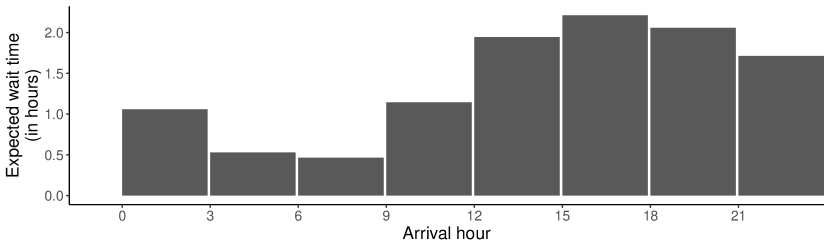
(b) Expected wait time throughout a day

(c) Expected service time throughout a day

Figure 2: Summary of the numeric variables

Table 3: Summary of the categorical variables

Category	Proportion
Gender
Female	60%
Male	40%
Race
African American or Black	56%
American Indian or Alaskan Native	0.25%
Asian	3.0%
Caucasian or White	39%
Hispanic	$<0.1$%
Multiple	0.35%
Native Hawaiian or Other Pacific Islander	0.11%
Unknown, Unavailable or Unreported	1.5%
Main complaint category
Cardio	17%
Gastro	13%
General	19%
Neurology	5.6%
Non-Traumatic	6.3%
Other	32%
Trauma	6.9%

Figure 3 displays the histograms of service times of patients upon entering a bed in the ED treatment ward, to until completion of treatment. The histograms are bucketed by time of arrival, and the red dotted lines overlaid onto each plot represent the fitted log-normal distributions.

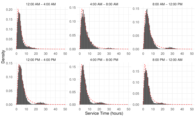
Figure 3: Log-normal density fits (red dashed lines) overlaid on the empirical histograms of service times conditional on time of arrival.

9 Experiments

9.1 Patient Satisfaction

As part of patient satisfaction drive, hospitals are increasingly providing individualized wait time forecasts to patients. However, patients appear to exhibit loss aversion regarding ED wait times, where the discomfort of longer-than-anticipated waits outweighs the gains from shorter-than-expected waits (Ansari et al. 2022). This asymmetry suggests that patients are more satisfied when they are provided with conservative estimates that correspond to a high percentile of their wait time distribution, which Ansari et al. (2022) identified as the 70th percentile. Thus we model patient dissatisfaction with the quantile loss

$$\mathcal{L}_{\alpha}(y,\hat{y})=\begin{cases}\alpha(y-\hat{y})&\text{if }y-\hat{y}\geq 0\\ (1-\alpha)(\hat{y}-y)&\text{otherwise}\end{cases},$$

which is minimized by setting the prediction $\hat{y}$ to the $100\alpha$th percentile of the distribution of $y$. The 70th percentile corresponds to an underage-to-overage cost ratio of $0.7/(1-0.3)=2.3$. In Table 4 we evaluate how dissatisfied patients are with the percentile predictions from the proposed and benchmark models: Out-of-sample quantile loss values are presented for a range of $\alpha$-values centred around $0.7$. bGND consistently reduces patient dissatisfaction by 8-10% over QRF across the range of percentiles considered.

We also present the performances of three more approaches. Boosted GLM is the linear boosting approach used in Ansari et al. (2022). They convert their point estimates to quantiles using a $t$-distribution with homoskedastic standard errors. The classic exponential model specifies the log-rate parameter linearly in the covariates. Finally, we include a naive benchmark called Historical Average, which simply divides a week into 21 bins so that each day of the week consists of three eight-hour bins. Historical average wait time within these bins is used as a point estimate.

Table 4: Out-of-sample quantile loss by target percentiles

Percentile Cost Ratio bGND QRF Boosted GLM Classic Exponential Hist. Avg. 60 1.5 0.51 0.57 0.60 0.54 0.63 65 1.9 0.51 0.57 0.73 0.54 0.62 70 2.3 0.50 0.55 0.95 0.53 0.60 75 3.0 0.47 0.52 1.28 0.51 0.58 80 4.0 0.44 0.47 1.74 0.47 0.56

• Notes: All figures are rounded to two significant digits.

9.2 Reduction in mortality following cardiac arrest

For patients suffering from myocardial infarction, Boersma et al. (1996) identified a 2.8 percentage point lower mortality rate when treatment is administered within the golden hour, compared with commencing treatment in the second hour. We conduct a stylized analysis where the ED can identify patients who will wait more than 10 minutes and we call these long waits. To this end, we focus on patients who showed up with chest pain complaints in our data. We set the 10-minute cutoff assuming the travel time to the ED and conducting tests after the wait time would take up to 50 minutes in total. In this classification task, we employ varying thresholds for flagging a patient as being at-risk of waiting for more than 10 minutes. As an example, if the threshold is 5%, we would flag patients whose forecasted probability of waiting for more than 10 minutes is amongst the top 5 percent of forecasts. This approach reflects a capacity constraint on the ED, which can only prioritize a finite number of patients. The top half of Table 5 presents out-of-sample true positive rates achieved when we threshold the top 5%, 10%, …, 25% of patient forecasts.

We also present out-of-sample mortality reductions achieved by the proposed and alternative forecasts in the bottom half of Table 5. We assume that the ED can reduce mortality rate by 2.8 percentage points if the patient is correctly identified as a long wait. Therefore, the overall reduction in mortality rate is the true positive rate multiplied by 0.028. In Table 5, we convert the reduction in mortality rate into the number of deaths averted. In the United States, every year, approximately 805,000 people have a heart attack (Tsao et al. 2022).

Table 5: Identifying long waits among ED visits with chest pain complaints

% of population bGND QRF Boosted GLM Classic Exponential Hist. Avg. True positive rate    5 0.98 0.95 0.95 0.93 0.83    10 0.97 0.94 0.94 0.92 0.83    15 0.96 0.93 0.93 0.92 0.83    20 0.96 0.92 0.93 0.92 0.83    25 0.95 0.92 0.92 0.92 0.83 Reduction in mortality    5 1,100 1,100 1,100 1,000 930    10 2,200 2,100 2,100 2,100 1,900    15 3,300 3,100 3,100 3,100 2,800    20 4,300 4,200 4,200 4,100 3,800    25 5,400 5,200 5,200 5,200 4,700

• Notes: Identifying patients at-risk of not receiving treatment within the golden hour, so that the ED can prioritize them. All figures are rounded to two significant digits.

References

• Alley et al. (2023) Alley M, Biggs M, Hariss R, Herrmann C, Li ML, Perakis G (2023) Pricing for heterogeneous products: Analytics for ticket reselling. Manufacturing & Service Operations Management 25(2):409–426.
• Ansari et al. (2022) Ansari S, Debo L, Ibanez M, Iravani S, Malik S MD (2022) Under-promising and over-delivering to improve patient satisfaction at emergency departments: Evidence from a field experiment providing wait information. Available at SSRN: https://ssrn.com/abstract=4135705.
• Armony et al. (2015) Armony M, Israelit S, Mandelbaum A, Marmor YN, Tseytlin Y, Yom-Tov GB (2015) On patient flow in hospitals: A data-based queueing-science perspective. Stochastic systems 5(1):146–194.
• Arora et al. (2023) Arora S, Taylor JW, Mak HY (2023) Probabilistic forecasting of patient waiting times in an emergency department. Manufacturing & Service Operations Management 25(4):1489–1508.
• Ban and Rudin (2019) Ban GY, Rudin C (2019) The big data newsvendor: Practical insights from machine learning. Operations Research 67(1):90–108.
• Bertsimas and Kallus (2020) Bertsimas D, Kallus N (2020) From predictive to prescriptive analytics. Management Science 66(3):1025–1044.
• Bertsimas et al. (2016) Bertsimas D, O’Hair A, Relyea S, Silberholz J (2016) An analytics approach to designing combination chemotherapy regimens for cancer. Management Science 62(5):1511–1531.
• Bertsimas et al. (2022) Bertsimas D, Pauphilet J, Stevens J, Tandon M (2022) Predicting inpatient flow at a major hospital using interpretable analytics. Manufacturing & Service Operations Management 24(6):2809–2824.
• Bickel (1982) Bickel PJ (1982) On adaptive estimation. Annals of Statistics 10(3):647–671.
• Boersma et al. (1996) Boersma E, Maas AC, Deckers JW, Simoons ML (1996) Early thrombolytic treatment in acute myocardial infarction: reappraisal of the golden hour. The Lancet 348(9030):771–775.
• Box and Cox (1964) Box GE, Cox DR (1964) An analysis of transformations. Journal of the Royal Statistical Society Series B: Statistical Methodology 26(2):211–243.
• Brown et al. (2005) Brown L, Gans N, Mandelbaum A, Sakov A, Shen H, Zeltyn S, Zhao L (2005) Statistical analysis of a telephone call center: A queueing-science perspective. Journal of the American Statistical Association 100(469):36–50.
• Chan et al. (2017) Chan CW, Farias VF, Escobar GJ (2017) The impact of delays on service times in the intensive care unit. Management Science 63(7):2049–2072.
• Chen et al. (2024) Chen N, Gürlek R, Lee DKK, Shen H (2024) Can customer arrival rates be modelled by sine waves? Service Science 16(2):70–84.
• Chen et al. (2019) Chen N, Lee DKK, Negahban SN (2019) Super-resolution estimation of cyclic arrival rates. Annals of Statistics 47(3):1754–1775.
• Chen et al. (2023) Chen W, Argon NT, Bohrmann T, Linthicum B, Lopiano K, Mehrotra A, Travers D, Ziya S (2023) Using hospital admission predictions at triage for improving patient length of stay in emergency departments. Operations Research 71(5):1733–1755.
• Ding et al. (2024) Ding H, Sokol T, Kc D, Lee DKK (2024) Valuing nursing productivity in emergency departments. Manufacturing & Service Operations Management (forthcoming) .
• Duan et al. (2020) Duan T, Anand A, Ding DY, Thai KK, Basu S, Ng A, Schuler A (2020) Ngboost: Natural gradient boosting for probabilistic prediction. International Conference on Machine Learning, 2690–2700 (PMLR).
• Elmachtoub and Grigas (2022) Elmachtoub AN, Grigas P (2022) Smart “predict, then optimize”. Management Science 68(1):9–26.
• Friedman (2001) Friedman JH (2001) Greedy function approximation: A gradient boosting machine. Annals of Statistics 1189–1232.
• Gneiting and Raftery (2007) Gneiting T, Raftery AE (2007) Strictly proper scoring rules, prediction, and estimation. Journal of the American statistical Association 102(477):359–378.
• Hawkins and Wixley (1986) Hawkins DM, Wixley R (1986) A note on the transformation of chi-squared variables to normality. The American Statistician 40(4):296–298.
• He et al. (2012) He B, Dexter F, Macario A, Zenios S (2012) The timing of staffing decisions in hospital operating rooms: incorporating workload heterogeneity into the newsvendor problem. Manufacturing & Service Operations Management 14(1):99–114.
• Kingman (1962) Kingman JF (1962) On queues in heavy traffic. Journal of the Royal Statistical Society: Series B 24(2):383–392.
• Ledoux and Talagrand (1991) Ledoux M, Talagrand M (1991) Probability in Banach Spaces: isoperimetry and processes (Springer NY).
• Lee et al. (2021) Lee DKK, Chen N, Ishwaran H (2021) Boosted nonparametric hazards with time-dependent covariates. Annals of Statistics 49(4):2101–2128.
• Liu et al. (2021) Liu S, He L, Max Shen ZJ (2021) On-time last-mile delivery: Order assignment with travel-time predictors. Management Science 67(7):4095–4119.
• Lowsky et al. (2018) Lowsky DJ, Lee DKK, Zenios SA (2018) Health savings accounts: Consumer contribution strategies and policy implications. MDM Policy & Practice 3(2):2381468318809373.
• März and Kneib (2022) März A, Kneib T (2022) Distributional gradient boosting machines. arXiv preprint arXiv:2204.00778 .
• Meinshausen (2006) Meinshausen N (2006) Quantile regression forests. Journal of Machine Learning Research 7(6):983–999.
• Niewoehner III et al. (2023) Niewoehner III RJ, Diwas K, Staats B (2023) Physician discretion and patient pick-up: How familiarity encourages multitasking in the emergency department. Operations Research 71(3):958–978.
• Notz and Pibernik (2022) Notz PM, Pibernik R (2022) Prescriptive analytics for flexible capacity management. Management Science 68(3):1756–1775.
• Raissi et al. (2019) Raissi M, Perdikaris P, Karniadakis GE (2019) Physics-informed neural networks: A deep learning framework for solving forward and inverse problems involving nonlinear partial differential equations. Journal of Computational physics 378:686–707.
• Rath et al. (2017) Rath S, Rajaram K, Mahajan A (2017) Integrated anesthesiologist and room scheduling for surgeries: Methodology and application. Operations Research 65(6):1460–1478.
• Senoner et al. (2022) Senoner J, Netland T, Feuerriegel S (2022) Using explainable artificial intelligence to improve process quality: Evidence from semiconductor manufacturing. Management Science 68(8):5704–5723.
• Shi et al. (2016) Shi P, Chou MC, Dai JG, Ding D, Sim J (2016) Models and insights for hospital inpatient operations: Time-dependent ed boarding time. Management Science 62(1):1–28.
• Singh et al. (2024) Singh S, Gurvich I, Mieghem JAV (2024) Feature-driven priority queuing. SSRN Electronic Journal URL https://ssrn.com/abstract=3731865.
• Song et al. (2015) Song H, Tucker AL, Murrell KL (2015) The diseconomies of queue pooling: An empirical investigation of emergency department length of stay. Management Science 61(12):3032–3053.
• Tsao et al. (2022) Tsao CW, Aday AW, Almarzooq ZI, Alonso A, Beaton AZ, Bittencourt MS, Boehme AK, Buxton AE, Carson AP, Commodore-Mensah Y, et al. (2022) Heart disease and stroke statistics—2022 update: a report from the american heart association. Circulation 145(8):e153–e639.
• van der Vaart and Wellner (1996) van der Vaart AW, Wellner JA (1996) Weak convergence and empirical processes with applications to statistics (Springer NY).
• Westgate et al. (2013) Westgate BS, Woodard DB, Matteson DS, Henderson SG (2013) Travel time estimation for ambulances using bayesian data augmentation. The Annals of Applied Statistics 1139–1161.
• Zhang and Yu (2005) Zhang T, Yu B (2005) Boosting with early stopping: Convergence and consistency. Annals of Statistics 33(4):1538–1579.
\ECSwitch
\ECHead