Stochastic Gene Expression Model of Nuclear-to-Cell Ratio Homeostasis

Abstract.

Cell size varies between different cell types, and between different growth and osmotic conditions. However, the nuclear-to-cell volume ratio (N/C ratio) remains nearly constant. In this paper, we build on existing deterministic models of N/C ratio homeostasis and develop a simplified gene translation model to study the effect of stochasticity on the N/C ratio homeostasis. We solve the corresponding chemical master equation and obtain the mean and variance of the N/C ratio. We also use a Taylor expansion approximation to study the effects of the system size on the fluctuations of the N/C ratio. We then combine the translation model with a cell division model to study the effects of extrinsic noises from cell division on the N/C ratio. Our model demonstrates that the N/C ratio homeostasis is maintained when the stochasticity in cell growth is taken into account, that the N/C ratio is largely determined by the gene fraction of nuclear proteins, and that the fluctuations in the N/C ratio diminish as the system size increases.

1. Introduction and background

1.1. Introduction

Cell size varies among different cell types, and within the same cell type, cell size may vary significantly under different growth and osmotic conditions. However, it has long been observed that the size of the nucleus scales with cell size so that the nuclear-to-cytoplasmic volume ratio (N/C ratio for short) remains nearly constant [9, 29, 32]. The N/C ratio has been hypothesized to regulate developmental timing such as the zygotic genome activation in early embryo development [36], and may be crucial in the origin of animal multicellularity [8, 33]. Because the N/C ratio is maintained when the number of genomes within a cell (ploidy) is manipulated [3], it is unlikely that the N/C ratio is determined by DNA content, and the mechanism for the determination of the N/C ratio remains an active field of study.

A simple osmotic pressure balance model was proposed in [5, 11, 27] that provides a physical basis for the N/C ratio. The model is based on the balance of osmotic pressure at the nuclear envelope and the cell membrane, and it shows that the N/C ratio is effectively determined by the ratio between the osmolyte numbers in the nucleus and the cytoplasm. However, the cellular mechanism that makes this osmolyte number ratio insensitive to perturbations is still poorly understood [35].

During cell growth, an N/C ratio homeostasis is maintained dynamically, where aberrant N/C ratios are corrected over time. A macroscopic growth model based on an active feedback mechanism was proposed in [7], whereas our previous work [27] showed that the N/C ratio homeostasis can be explained by a growth model without active feedback. More detailed growth models that take into account the nucleocytoplasmic transport have also been proposed [5, 41]. To the best of our knowledge, all these previous growth models explaining the N/C ratio homeostasis are deterministic. Given that the process of cell growth, including mRNA transcription and protein translation, are stochastic in nature [37], it is important to study the effects of stochasticity on the N/C ratio.

In this paper, we develop a stochastic cell growth model to study the N/C ratio homeostasis, which is based on an existing stochastic gene expression model [28]. We solve the corresponding chemical master equation (CME) to obtain a time-dependent joint probability distribution of the random variables. We then use this probability distribution to calculate the mean and variance of the N/C ratio and show the N/C ratio homeostasis is maintained in this stochastic model. Finally, we use a Taylor expansion approximation of the N/C ratio to study how the system size affects the fluctuations of the N/C ratio, and show that the fluctuations are predicted to diminish as the system size grow.

The major challenge faced in this study is solving the CME. To the best of our knowledge, while it is possible to analytically solve the CMEs corresponding to general systems of first order (monomolecular) reactions [23, 34, 39], for second order (bimolecular) reactions and beyond, analytical solutions of the CMEs corresponding to general reaction systems are unavailable except for certain special cases [25, 26]. Various numerical methods are available to compute approximate solutions, such as the Gillespie algorithm [17, 18], Galerkin spectral methods [13, 14, 15], and finite space projection methods [31]. Analytical approximation methods for CMEs are also known, such as the chemical Langevin equations, the Fokker-Planck equations, and the system size expansion [16, 38].

In this paper, we use a minimal stochastic cell growth model in which all reactions are first order, which allows us to use a Fourier transform method [34] to solve the CME. We achieve this relative simplicity by modeling the translation process only, instead of modeling both the transcription and the translation process. We use a coarse-grained model for the translation process that does not attempt to capture in detail the various cell biological processes involved in N/C ratio determination, such as nucleocytoplasmic transport. This minimal model allows us to capture salient aspects of N/C ratio homeostasis and provides a basis for more detailed stochastic models for the N/C ratio homeostasis in future studies.

We will explain how in this paper we (i) incorporate stochasticity into models of nuclear size control by osmotic force balance; (ii) obtain an expression for the dependence of the N/C ratio on system size in the limit of a large number of solutes.

1.2. Osmotic pressure balance model

Our starting point is the osmotic pressure balance model [5, 11, 27]. The basic assumptions of the osmotic pressure balance model are as follows:

1. The osmotic effect of chromatin is negligible;

2. The osmotic pressure is described by van’t Hoff’s law;

3. The tension at the nuclear envelope and the cell membrane is described by the Young-Laplace law.

The equations describing the osmotic pressure balance are

(1a) $$(c_{n}-c_{cyto})k_{B}T =\frac{2\sigma_{n}}{R_{n}};$$

(1b) $$(c_{cyto}-c_{0})k_{B}T =\frac{2\sigma_{cell}}{R_{cell}},$$

in which $c_{n}$, $c_{cyto}$, and $c_{0}$ are the total concentrations of solutes in the nucleus, the cytoplasm, and outside the cell; $\sigma_{n}$ and $\sigma_{cell}$ are the tensions in the nuclear envelope and the cell membrane; $R_{n}$ and $R_{cell}$ are the radii of the nucleus and the cell, respectively; $k_{B}$ is the Boltzmann constant; and $T$ is the temperature. If the further assumption is made that smaller osmolytes (e.g. ions and metabolites such as amino acids) freely diffuse across the nuclear envelope through nuclear pore complexes (NPCs), then only the concentrations of larger osmolytes (proteins and other macromolecules) are needed in the pressure balance of the nuclear envelope:

(2a) $$\left(\frac{p_{n}}{V_{n}-b_{n}}-\frac{p_{cyto}}{V_{cyto}-b_{cyto}}\right)k_{B}T =\frac{2\sigma_{n}}{R_{n}};$$

(2b) $$\left(\frac{p_{cyto}+n_{cyto}}{V_{cyto}-b_{cyto}}-c_{0}\right)k_{B}T =\frac{2\sigma_{cell}}{R_{cell}}.$$

Here $n_{cyto}$ is the number of smaller osmolytes in the cytoplasm, $p$ denotes the number of the larger osmolytes in the respective compartment, $V$ denotes the total volume, and $b$ denotes the non-osmotic volume. We note that we use $p$ to denote solute number throughout this manuscript. In particular, it does not denote the osmotic pressure.

In the case that the nuclear envelope is stress-free and $\sigma_{n}=0$, and that the non-osmotic volumes are negligible i.e. $b_{n}<<V_{n}$ and $b_{cyto}<<V_{cyto}$, the osmotic pressure balance equations simplify further [27] to

(3) $$\frac{p_{n}}{V_{n}}=\frac{p_{cyto}}{V_{cyto}},\quad\mbox{i.e.}\quad\frac{V_{n}}{V_{cyto}}=\frac{p_{n}}{p_{cyto}}:=NC_{cyto}.$$

Equation (3) implies that under the assumptions stated above, by van’t Hoff’s formula, the N/C ratio is determined solely by the ratio of protein numbers in the nucleus and the cytoplasm. Therefore, we may study the N/C ratio homeostasis problem by studying the mechanisms that maintains the homeostasis of the protein ratio.

1.3. A statistical viewpoint on the N/C ratio: stochastic gene translation models

We next study the N/C ratio homeostasis problem from a statistical viewpoint. More precisely, we formulate a stochastic model for the growth of protein numbers which not only captures the passive feedback mechanism that corrects aberrant N/C ratio values [27], but also explains the fluctuations in the N/C ratio over time.

Consider a biochemical reaction system representing a simplified process of gene expression, with the species of reactants listed below.

• Proteins: RNA polymerases (RNAPs) $P_{p}$, ribosomes $P_{r}$, nuclear proteins $P_{n}$, cytoplasmic proteins $P_{c}$;

• mRNAs: $M_{p}$, $M_{r}$, $M_{n}$, $M_{c}$, which corresponds to the above protein species;

• Genes: $G_{p}$, $G_{r}$, $G_{n}$, $G_{c}$, which corresponds to the above mRNA species.

Let $g_{i}$, $m_{i}$, $p_{i}$, $i=p,r,n,c$ denote the corresponding numbers of genes, mRNAs, and proteins, respectively.

We begin by considering the stochastic gene expression model of Lin and Amir [28], which assumes that the transcription (resp. translation) rate for a specific gene $i$ is proportional to the fraction of RNAPs (resp. ribosomes) bound to its genes (resp. mRNAs), $\phi_{i}=\dfrac{g_{i}}{\sum g_{i}}$ (resp. $f_{i}=\dfrac{m_{i}}{\sum m_{i}}$):

(4a) $$\emptyset \xrightarrow{k_{0}\frac{g_{i}}{\sum g_{i}}p_{p}}M_{i},\quad i=p,r,n,c\quad\mbox{(transcription);}$$

(4b) $$\emptyset \xrightarrow{k_{t}\frac{m_{i}}{\sum m_{i}}p_{r}}P_{i},\quad i=p,r,n,c\quad\mbox{(translation);}$$

(4c) $$M_{i} \xrightarrow{\frac{1}{\tau}}\emptyset,\quad i=p,r,n,c\quad\mbox{(mRNA degredation).}$$

1.4. A simplified gene translation model

We seek to obtain a complete time-dependent joint probability distribution of the random variables in the model. However, in the above transcription and translation model, the reaction rates are time-dependent, which makes the model difficult to solve analytically. Therefore, we consider the following simplified model of translation, which assumes that the translation rate for each protein is directly proportional to its gene fraction:

(5a) $$P_{r} \xrightarrow{k_{r}}2P_{r},\quad k_{r}=k_{t}\phi_{r}\quad\mbox{(autocatalytic synthesis of ribosomes)};$$

(5b) $$P_{r} \xrightarrow{k_{n}}P_{r}+P_{n},\quad k_{n}=k_{t}\phi_{n}\quad\mbox{(translation of nuclear proteins)};$$

(5c) $$P_{r} \xrightarrow{k_{c}}P_{r}+P_{c},\quad k_{c}=k_{t}\phi_{c}\quad\mbox{(translation of cytoplasmic proteins)}.$$

Because this reaction system involves only first-order reactions with time-independent reaction rates, its CME may be solved analytically.

Comparing the simplified model (5) with the original model (4), we see that to assume the translation rate $k_{i}=k_{t}\phi_{i}$ means to assume that the mRNA fractions $f_{i}$ are equal to their corresponding gene fractions $\phi_{i}$.

1.5. Nuclear-to-cytoplasmic ratio and nuclear-to-cell ratio

We first note that in the literature, the N/C ratio usually denotes a ratio between volumes. However, as we have seen from (3), under the assumptions of our osmotic pressure balance model, the ratio between volumes is equal to the ratio of the corresponding protein numbers. Therefore, from this section on, we will focus on the ratio between protein numbers unless otherwise specified.

We note further that the N/C ratio may either refer in the literature to the nuclear-to-cell ratio ($NC_{cell}$) or the nuclear-to-cytoplasmic ratio ($NC_{cyto}$). To clarify, we define $NC_{cyto}$ to be the ratio between the number of nuclear proteins and the total number of cytoplasmic proteins, as in (3):

$$NC_{cyto}=\frac{p_{n}}{p_{r}+p_{c}},$$

and we define $NC_{cell}$ to be the ratio between the number of nuclear proteins and the total number of proteins in the cell:

$$NC_{cell}=\frac{p_{n}}{p_{r}+p_{n}+p_{c}}.$$

We will focus on $NC_{cell}$ here as in our previous work [27], although by (3) it may be more convenient in some cases to use $NC_{cyto}$, e.g. when discussing the osmotic balance across the nuclear envelope.

The main results to be shown in this paper are as follows:

1. We show that $NC_{cell}$ is determined by the ratios of gene fractions $\frac{\phi_{n}}{\phi_{r}+\phi_{n}+\phi_{c}}=\phi_{n}$, where $\phi_{i}=\frac{g_{i}}{\sum g_{i}}$, and $\phi_{r}+\phi_{n}+\phi_{c}=1$;

2. We show that $NC_{cell}$ will maintain a homeostasis; namely, if the initial conditions

   $$NC_{cell,0}=\frac{p_{n,0}}{p_{r,0}+p_{n,0}+p_{c,0}}$$

   deviate from $\phi_{n}$, then $NC_{cell}\to\phi_{n}$ as time $t\to\infty$;

3. We compute the mean, variance, and standard deviation of $NC_{cell}$; in particular, we show how the coefficient of variation $\frac{\mathrm{SD}(NCe)}{\langle NCe\rangle}$ decreases as the numbers of proteins $p_{r}$, $p_{n}$, and $p_{c}$ increase;

4. We determine the relationship between

   $$\langle NC_{cell}\rangle=\left\langle\frac{p_{n}}{p_{r}+p_{n}+p_{c}}\right\rangle\quad\mbox{and}\quad\frac{\langle p_{n}\rangle}{\langle p_{r}\rangle+\langle p_{n}\rangle+\langle p_{c}\rangle},$$

   where the former is the average of the ratio and the latter is the ratio of the average.

2. Methods

2.1. Chemical master equation corresponding to the simplified translation model

The CME corresponding to the reaction system (5) is

(6) $$\begin{split}&\frac{\partial}{\partial t}P(p_{r},p_{n},p_{c},t)\\ &=k_{r}(p_{r}-1)P(p_{r}-1,p_{n},p_{c},t)+k_{n}p_{r}P(p_{r},p_{n}-1,p_{c},t)+k_{c}p_{r}P(p_{r},p_{n},p_{c}-1)\\ &-(k_{r}+k_{n}+k_{c})p_{r}P(p_{r},p_{n},p_{c},t),\end{split}$$

where $P(p_{r},p_{n},p_{c},t)$ is the joint probability distribution of $p_{r}$, $p_{n}$, and $p_{c}$.

The CME (6) can be solved with different initial conditions. A straightforward choice is the deterministic initial condition: the numbers of proteins at $t=0$ are given deterministically by $p_{r,0}$, $p_{n,0}$, and $p_{c,0}$, and

(7) $$P(p_{r},p_{n},p_{c},0)=\delta_{p_{r}-p_{r,0}}\delta_{p_{n}-p_{n,0}}\delta_{p_{c}-p_{c,0}}.$$

Alternatively, the initial condition can be stochastic instead of deterministic. From a biological view point, stochastic initial conditions can be used to model the random partitioning of molecules at cell division. An example is the Poisson initial condition: the averages of protein numbers at $t=0$ are given by $\langle p_{r}(0)\rangle=p_{r,0}$, $\langle p_{n}(0)\rangle=p_{n,0}$, and $\langle p_{c}(0)\rangle=p_{c,0}$; if $p_{r}(0)$, $p_{n}(0)$, and $p_{c}(0)$ are assumed to be independently Poisson distributed, then

(8) $$P(p_{r},p_{n},p_{c},0)=\frac{p_{r,0}^{p_{r}}p_{n,0}^{p_{n}}p_{c,0}^{p_{c}}}{p_{r}!p_{n}!p_{c}!}e^{-(p_{r,0}+p_{n,0}+p_{c,0})}.$$

Other types of initial conditions, such as binomial initial condition, can also be applied.

In what follows, we will only consider deterministic initial conditions, and we will specify initial conditions for (6) with emphasis on the size of the reaction system, as well as the initial $NC_{cyto}$ and $NC_{cell}$ ratios. To do this, we introduce a system size variable $N$, as well as initial protein fractions $f_{r}$, $f_{n}$, $f_{c}$, corresponding to ribosomes, nuclear, and cytoplasmic proteins, respectively, so that the initial $NC_{cyto}$ and $NC_{cell}$ ratios are

$$NC_{cyto,0}=\frac{f_{n}}{f_{r}+f_{c}},\quad NC_{cell,0}=\frac{f_{n}}{f_{r}+f_{n}+f_{c}}.$$

(Note here that we do not require $f_{r}+f_{n}+f_{c}=1$.) Then $p_{r,0}$, $p_{n,0}$, and $p_{c,0}$ are given by

$$p_{r,0}=f_{r}N,\quad p_{n,0}=f_{n}N,\quad p_{c,0}=f_{c}N.$$

2.1.1. Solving the chemical master equation using the generating function and Fourier transform

The generating function for the joint distribution $P(p_{r},p_{n},p_{c},t)$ is defined as

(9) $$G(s_{r},s_{n},s_{c},t)=\sum_{p_{r}=0}^{\infty}\sum_{p_{n}=0}^{\infty}\sum_{p_{c}=0}^{\infty}P(p_{r},p_{n},p_{c},t)s_{r}^{p_{r}}s_{n}^{p_{n}}s_{c}^{p_{c}}.$$

We will solve (6) by first solving the partial differential equation (PDE) for the generating function. Using a well-known formula for generating function equations [16], we get the PDE for $G(s_{r},s_{n},s_{c},t)$:

(10) $$\frac{\partial}{\partial t}G(s_{r},s_{n},s_{c},t)=[k_{r}(s_{r}^{2}-s_{r})+k_{n}(s_{r}s_{n}-s_{r})+k_{c}(s_{r}s_{c}-s_{r})]\frac{\partial}{\partial s_{r}}G(s_{r},s_{n},s_{c},t),$$

with deterministic initial condition

(11) $$G(s_{r},s_{n},s_{c},0)=s_{r}^{p_{r,0}}s_{n}^{p_{n,0}}s_{c}^{p_{c,0}}.$$

For general reaction systems involving second or higher order reactions, the generating function equations are PDEs of at least second order, which, in general, cannot be solved analytically. However, since our reaction system (5) involves only first order reactions, the generating function equation (10) is a first order PDE and can thus be solved using the method of characteristics: the characteristic equations for (10) are

(12a) $$\frac{dt}{d\tau} =1,$$

(12b) $$\frac{ds_{r}}{d\tau} =-[k_{r}(s_{r}^{2}-s_{r})+k_{n}(s_{r}s_{n}-s_{r})+k_{c}(s_{r}s_{c}-s_{r})],$$

(12c) $$\frac{ds_{n}}{d\tau} =0,$$

(12d) $$\frac{ds_{c}}{d\tau} =0,$$

(12e) $$\frac{dG}{d\tau} =0.$$

(12a), (12c), (12d), and (12e) lead to the following results:

(13a) $$t =\tau,$$

(13b) $$s_{n} =s_{n,0},$$

(13c) $$s_{c} =s_{c,0},$$

(13d) $$G =s_{r,0}^{p_{r,0}}s_{n,0}^{p_{n,0}}s_{c,0}^{p_{c,0}}.\quad\mbox{(Deterministic I.C.)}$$

Now (12b) becomes

(14) $$\frac{ds_{r}}{dt}=-[k_{r}(s_{r}^{2}-s_{r})+k_{n}(s_{r}s_{n,0}-s_{r})+k_{c}(s_{r}s_{c,0}-s_{r})],$$

which is separable and can be solved by the method of partial fractions. The solution is given by

(15) $$s_{r}=\frac{-k_{r}s_{r,0}+k_{n}(s_{n,0}-1)s_{r,0}+k_{c}(s_{c,0}-1)s_{r,0}}{[k_{r}(s_{r,0}-1)+k_{n}(s_{n,0}-1)+k_{c}(s_{c,0}-1)]e^{[-k_{r}+k_{n}(s_{n,0}-1)+k_{c}(s_{c,0}-1)]t}-k_{r}s_{r,0}},$$

and then

(16) $$s_{r,0}=\frac{-k_{r}s_{r}+k_{n}(s_{n,0}-1)s_{r}+k_{c}(s_{c,0}-1)s_{r}}{[k_{r}(s_{r}-1)+k_{n}(s_{n,0}-1)+k_{c}(s_{c,0}-1)]e^{[k_{r}-k_{n}(s_{n,0}-1)-k_{c}(s_{c,0}-1)]t}-k_{r}s_{r}},$$

Putting everything together, we get an expression of the generating function corresponding to deterministic initial condition

(17) $$\begin{split}&G(s_{r},s_{n},s_{c},t)=\\ &\left[\frac{-k_{r}s_{r}+k_{n}(s_{n}-1)s_{r}+k_{c}(s_{c}-1)s_{r}}{[k_{r}(s_{r}-1)+k_{n}(s_{n}-1)+k_{c}(s_{c}-1)]e^{[k_{r}-k_{n}(s_{n}-1)-k_{c}(s_{c}-1)]t}-k_{r}s_{r}}\right]^{p_{r,0}}s_{n}^{p_{n,0}}s_{c}^{p_{c},0}.\end{split}$$

Now we can calculate $P(p_{r},p_{n},p_{c},t)$ by using the following Cauchy integral formula [34]:

(18) $$P(p_{r},p_{n},p_{c},t)=\frac{1}{(2\pi i)^{3}}\oint_{C_{r}\times C_{n}\times C_{c}}\frac{G(s_{r},s_{n},s_{c},t)}{s_{r}^{p_{r}+1}s_{n}^{p_{n}+1}s_{c}^{p_{c}+1}}ds_{r}ds_{n}ds_{c},$$

where $C_{i}$ are discs encircling the origin of the complex hyperplane. If we let $\psi(\theta_{r},\theta_{n},\theta_{c},t)=G(e^{2\pi i\theta_{r}},e^{2\pi i\theta_{n}},e^{2\pi i\theta_{c}},t)$, then (18) becomes

(19) $$P(p_{r},p_{n},p_{c},t)=\int_{[0,1]^{3}}\psi(\theta_{r},\theta_{n},\theta_{c},t)e^{-2\pi i\theta_{r}p_{r}}e^{-2\pi i\theta_{n}p_{n}}e^{-2\pi i\theta_{c}p_{c}}d\theta_{r}d\theta_{n}d\theta_{c},$$

which is the Fourier transform of $\psi(\theta_{r},\theta_{n},\theta_{c},t)$. Therefore, the analytical solution (19) of the CME (6) is given in terms of an integral rather than a closed-form solution. However, (19) can be conveniently evaluated numerically using, e.g. Matlab’s fftn.

2.1.2. Calculation of moments from the generating function

As a consequence of solving the CME (6) using the generating function and Fourier transform, the moments of the joint distribution can be conveniently calculated from the generating function (9) by taking the corresponding partial derivatives of the expression (17). These moments will later be used in the determination of grid sizes. For the first order moments (means) we have

(20) $$\left\langle p_{j}(t)\right\rangle=\frac{\partial}{\partial s_{j}}G(s_{r},s_{n},s_{c},t)\Big{|}_{s_{r}=s_{n}=s_{c}=1},\quad j=r,n,c.$$

As for the second order moments, we can calculate the variances by

(21) $$\left\langle(p_{j}(t))(p_{j}(t)-1)\right\rangle=\frac{\partial^{2}}{\partial s_{j}^{2}}G(s_{r},s_{n},s_{c},t)\Big{|}_{s_{r}=s_{n}=s_{c}=1},\quad j=r,n,c$$

so that

(22) $$\left\langle p_{j}^{2}(t)\right\rangle=\frac{\partial^{2}}{\partial s_{j}^{2}}G(s_{r},s_{n},s_{c},t)\Big{|}_{s_{r}=s_{n}=s_{c}=1}+\left\langle p_{j}(t)\right\rangle,\quad j=r,n,c;$$

and for the covariances we have

(23) $$\left\langle p_{j}(t)p_{k}(t)\right\rangle=\frac{\partial^{2}}{\partial s_{j}\partial s_{k}}G(s_{r},s_{n},s_{c},t)\Big{|}_{s_{r}=s_{n}=s_{c}=1},\quad j,k=r,n,c.$$

In principle, higher order moments can be calculated in a similar manner, although the expressions would be considerably more complicated.

2.1.3. Memory space problem and variable grid size method

A major challenge in the numerical implementation of (19) is that the solution process described above is memory intensive. Suppose that a uniform grid is used and that the number of grid points for each dimension in fftn is $N_{g}$. Then we would need a complex 3D array of dimension $N_{g}\times N_{g}\times N_{g}$ to represent the discretized $\psi(\theta_{r},\theta_{n},\theta_{c},t)$, which would occupy $16N_{g}^{3}$ Bytes of memory space. Therefore, the memory usage grows rapidly when $N$ increases. For example, when $N_{g}=1,024$, the memory usage is 16GB, which still lies within the capability of most desktop or laptop computers; whereas when $N_{g}=2,048$, the memory usage increases to 128GB, which is beyond the capability of many desktop computers (or even the capability of some high performance computing clusters).

In order to make the memory allocation more efficient, we proposed a variable grid size based on Chebyshev’s inequality which assigns different number of grid points for each dimension, and also make the grid numbers vary with time $t$ to account for the evolution of the probability distribution. That is, instead of a uniform grid, we allow the grid sizes in each dimension to be different and time-dependent, so that the dimension of the 3D array is $N_{r}(t)\times N_{n}(t)\times N_{c}(t)$, and

(24) $$N_{j}(t)=\mbox{{ceileven}}(\langle p_{j}(t)\rangle+N_{SD}\mathrm{SD}(p_{j}(t))),$$

where the function ceileven$(u)$ means rounding $u$ to the nearest even integer greater than or equal to $u$, and $N_{SD}$ is the number of standard deviations away from the mean. Note that $N_{j}(t)$’s need to be even in order for proper implementation of fftn. By Chebyshev’s inequality, taking $N_{SD}=8$ will yield a grid that covers at least 98% of the distribution. The means $\langle p_{j}(t)\rangle$ and standard deviations $\mathrm{SD}(p_{j}(t))$ can be calculated from (20) and (22) without knowing the full solution of the CME.

2.1.4. Calculation of the mean and variance of the N/C ratio

Once the joint distribution $P(p_{r},p_{n},p_{c},t)$ is obtained, we can directly compute the first and second moment of $NC_{cell}$ by

(25a) $$\langle NC_{cell}(t)\rangle =\left\langle\frac{p_{n}(t)}{p_{r}(t)+p_{n}(t)+p_{c}(t)}\right\rangle=\sum_{\begin{subarray}{c}p_{r}\geqslant 0,p_{n}\geqslant 0,p_{c}\geqslant 0\\ p_{r}+p_{n}+p_{c}\neq 0\end{subarray}}\frac{p_{n}}{p_{r}+p_{n}+p_{c}}P(p_{r},p_{n},p_{c},t),$$

(25b) $$\langle NC_{cell}(t)^{2}\rangle =\left\langle\left(\frac{p_{n}(t)}{p_{r}(t)+p_{n}(t)+p_{c}(t)}\right)^{2}\right\rangle=\sum_{\begin{subarray}{c}p_{r}\geqslant 0,p_{n}\geqslant 0,p_{c}\geqslant 0\\ p_{r}+p_{n}+p_{c}\neq 0\end{subarray}}\left(\frac{p_{n}}{p_{r}+p_{n}+p_{c}}\right)^{2}P(p_{r},p_{n},p_{c},t).$$

The means are then equal to the first moments, while the variances are then calculated by

(26) $$\mathrm{Var}(NC_{cell}(t))=\langle NC_{cell}^{2}(t)\rangle-\langle NC_{cell}(t)\rangle^{2}.$$

2.2. Taylor expansion approximation of the N/C ratio

It is possible to approximate the mean and variance of $NC_{cell}$ and $NC_{cyto}$ without calculating the joint probability distribution. This is done by using the bivariate Taylor expansion of the ratio function [12]. A brief description of the method is given as follows.

Consider two general random variables $x_{1}$, $x_{2}$, where $x_{2}\neq 0$. Let $f(x_{1},x_{2})=\dfrac{x_{1}}{x_{2}}$ be the ratio of the two variables. The formal Taylor expansion $T(x_{1},x_{2})$ of $f(x_{1},x_{2})$ around the mean values $(\mu_{1},\mu_{2})=\left(\langle x_{1}\rangle,\langle x_{2}\rangle\right)$ is

(27) $$T(x_{1},x_{2})=\sum_{\alpha_{1}+\alpha_{2}\geqslant 0}\frac{\partial^{\alpha_{1}+\alpha_{2}}f(\mu_{1},\mu_{2})}{\partial x_{1}^{\alpha_{1}}\partial x_{2}^{\alpha_{2}}}\frac{(x_{1}-\mu_{1})^{\alpha_{1}}(x_{2}-\mu_{2})^{\alpha_{2}}}{\alpha_{1}!\alpha_{2}!}.$$

Then the mean of the ratio $\left\langle\dfrac{x_{1}}{x_{2}}\right\rangle=\left\langle f(x_{1},x_{2})\right\rangle$ can be calculated formally by the taking mean of the Taylor expansion:

(28) $$\left\langle f(x_{1},x_{2})\right\rangle=\left\langle T(x_{1},x_{2})\right\rangle=\sum_{\alpha_{1}+\alpha_{2}\geqslant 0}\frac{\partial^{\alpha_{1}+\alpha_{2}}f(\mu_{1},\mu_{2})}{\partial x_{1}^{\alpha_{1}}\partial x_{2}^{\alpha_{2}}}\frac{\left\langle(x_{1}-\mu_{1})^{\alpha_{1}}(x_{2}-\mu_{2})^{\alpha_{2}}\right\rangle}{\alpha_{1}!\alpha_{2}!},$$

where $\left\langle(x_{1}-\mu_{1})^{\alpha_{1}}(x_{2}-\mu_{2})^{\alpha_{2}}\right\rangle$ are the mixed central moments of order $\alpha_{1}+\alpha_{2}$.

To obtain an approximation of the variance of the ratio

$$\mathrm{Var}\left(\dfrac{x_{1}}{x_{2}}\right)=\mathrm{Var}(f(x_{1},x_{2}))=\left\langle f(x_{1},x_{2})^{2}\right\rangle-\left\langle f(x_{1},x_{2})\right\rangle^{2},$$

we need to first calculate formally $\left\langle f(x_{1},x_{2})^{2}\right\rangle$ using the square of the formal Taylor expansion:

(29) $$T(x_{1},x_{2})^{2}$$

$$=\sum_{\alpha_{1}+\alpha_{2}\geqslant 0}\sum_{\beta_{1}+\beta_{2}\geqslant 0}\frac{\partial^{\alpha_{1}+\alpha_{2}}f(\mu_{1},\mu_{2})}{\partial x_{1}^{\alpha_{1}}\partial x_{2}^{\alpha_{2}}}\frac{\partial^{\beta_{1}+\beta_{2}}f(\mu_{1},\mu_{2})}{\partial x_{1}^{\beta_{1}}\partial x_{2}^{\beta_{2}}}\frac{(x_{1}-\mu_{1})^{\alpha_{1}+\beta_{1}}(x_{2}-\mu_{2})^{\alpha_{2}+\beta_{2}}}{\alpha_{1}!\alpha_{2}!\beta_{1}!\beta_{2}!},$$

so that

(30) $$\begin{split}&\left\langle f(x_{1},x_{2})^{2}\right\rangle=\left\langle T(x_{1},x_{2})^{2}\right\rangle\\ &=\sum_{\alpha_{1}+\alpha_{2}\geqslant 0}\sum_{\beta_{1}+\beta_{2}\geqslant 0}\frac{\partial^{\alpha_{1}+\alpha_{2}}f(\mu_{1},\mu_{2})}{\partial x_{1}^{\alpha_{1}}\partial x_{2}^{\alpha_{2}}}\frac{\partial^{\beta_{1}+\beta_{2}}f(\mu_{1},\mu_{2})}{\partial x_{1}^{\beta_{1}}\partial x_{2}^{\beta_{2}}}\frac{\left\langle(x_{1}-\mu_{1})^{\alpha_{1}+\beta_{1}}(x_{2}-\mu_{2})^{\alpha_{2}+\beta_{2}}\right\rangle}{\alpha_{1}!\alpha_{2}!\beta_{1}!\beta_{2}!},\end{split}$$

where, again, $\left\langle(x_{1}-\mu_{1})^{\alpha_{1}+\beta_{1}}(x_{2}-\mu_{2})^{\alpha_{2}+\beta_{2}}\right\rangle$ are the mixed central moments of order $\alpha_{1}+\alpha_{2}+\beta_{1}+\beta_{2}$. The variance is then given by

(31) $$\mathrm{Var}(f(x_{1},x_{2}))=\mathrm{Var}(T(x_{1},x_{2}))=\left\langle T(x_{1},x_{2})^{2}\right\rangle-\left\langle T(x_{1},x_{2})\right\rangle^{2}$$

From (28) and (30) we see that, in principle, as long as we can calculate (or approximately calculate) all the mixed central moments $\left\langle(x_{1}-\mu_{1})^{\gamma_{1}}(x_{2}-\mu_{2})^{\gamma_{2}}\right\rangle$, we can then calculate Taylor expansion approximations of the mean and variance of the ratio. In practice, however, higher order moments tend to be difficult to calculate. Therefore, we will only implement Taylor expansion approximations of order up to 2. Later, we will see that for calculating approximations of the mean and variance of $NC_{cell}$, these low order approximations work well compared to the more accurate results obtained from the joint probability distributions.

For the mean $\left\langle\dfrac{x_{1}}{x_{2}}\right\rangle$ of the ratio, it is feasible to calculate the Taylor expansion approximation up to the second order. However, we will start by looking at the first order approximation: letting $\alpha_{1}+\alpha_{2}\leqslant 1$ and substituting the partial derivatives of $f(x_{1},x_{2})=\dfrac{x_{1}}{x_{2}}$ into (28), we get

(32) $$\left\langle\dfrac{x_{1}}{x_{2}}\right\rangle\approx\frac{\mu_{1}}{\mu_{2}}=\frac{\langle x_{1}\rangle}{\langle x_{2}\rangle}.$$

This shows that the first order Taylor expansion approximation of the mean of the ratio is simply the ratio of the means. A more accurate result can be achieved by the second order approximation: letting $\alpha_{1}+\alpha_{2}\leqslant 2$ and substituting the partial derivatives of $f(x_{1},x_{2})=\dfrac{x_{1}}{x_{2}}$ into (28) again, we get

(33) $$\begin{split}\left\langle\dfrac{x_{1}}{x_{2}}\right\rangle&\approx\frac{\mu_{1}}{\mu_{2}}-\frac{\left\langle(x_{1}-\mu_{1})(x_{2}-\mu_{2})\right\rangle}{\mu_{2}^{2}}+\frac{\left\langle(x_{2}-\mu_{2})^{2}\right\rangle\mu_{1}}{\mu_{2}^{3}}\\ &=\frac{\langle x_{1}\rangle}{\langle x_{2}\rangle}-\frac{\mathrm{Cov}(x_{1},x_{2})}{\langle x_{2}\rangle^{2}}+\frac{\mathrm{Var}(x_{2})\langle x_{1}\rangle}{\langle x_{2}\rangle^{3}}.\end{split}$$

For the variance $\mathrm{Var}\left(\dfrac{x_{1}}{x_{2}}\right)$ of the ratio, it is only feasible to calculate the Taylor expansion approximation up to the first order, due to the complexity of the expression (30). In this case, we will also use the first order approximation (32) of the mean in the final calculation of the variance (31). The expression of the first order Taylor expansion approximation of $\mathrm{Var}\left(\dfrac{x_{1}}{x_{2}}\right)$ is

(34) $$\begin{split}\mathrm{Var}\left(\dfrac{x_{1}}{x_{2}}\right)&\approx\frac{\left\langle(x_{1}-\mu_{1})^{2}\right\rangle}{\mu_{2}^{2}}-\frac{2\left\langle(x_{1}-\mu_{1})(x_{2}-\mu_{2})\right\rangle\mu_{1}}{\mu_{2}^{3}}+\frac{\left\langle(x_{2}-\mu_{2})^{2}\right\rangle\mu_{1}^{2}}{\mu_{2}^{4}}\\ &=\frac{\mu_{1}^{2}}{\mu_{2}^{2}}\left[\frac{\left\langle(x_{1}-\mu_{1})^{2}\right\rangle}{\mu_{1}^{2}}-\frac{2\left\langle(x_{1}-\mu_{1})(x_{2}-\mu_{2})\right\rangle}{\mu_{1}\mu_{2}}+\frac{\left\langle(x_{2}-\mu_{2})^{2}\right\rangle}{\mu_{2}^{2}}\right]\\ &=\frac{\langle x_{1}\rangle^{2}}{\langle x_{2}\rangle^{2}}\left[\frac{\mathrm{Var}(x_{1})}{\langle x_{1}\rangle^{2}}-\frac{2\mathrm{Cov}(x_{1},x_{2})}{\langle x_{1}\rangle\langle x_{2}\rangle}+\frac{\mathrm{Var}(x_{2})}{\langle x_{2}\rangle^{2}}\right].\end{split}$$

3. Results

3.1. Closed-form expression of moments

As a by-product of the FFT method, we obtain closed-form expressions of the generating functions corresponding to the CME (6) with deterministic initial conditions (17), from which we can derive closed form expressions for the moments of the variables $p_{r}$, $p_{n}$, and $p_{c}$. These closed form expressions will play a key role later in the Taylor series expansion approximation of the $NC_{cell}$ curves.

All the expressions of moments are calculated from symbolic differentiations of the generating function (17), using Matlab’s Symbolic Toolbox.

It should be noted that these expressions can also be calculated by solving the ordinary differential equations (ODEs) for the moments, where the ODEs themselves are derived using the generating function equation (10) and (20), (22), (23), or using the Kramers-Moyal expansion [16, 38].

3.1.1. First order moments: means of protein numbers

Using (20), we can calculate the first order moments, that is, the means of each individual variable, as functions of time. For the mean of ribosome numbers we have

(35) $$\langle p_{r}(t)\rangle=p_{r,0}{e}^{k_{t}\phi_{r}t}=f_{r}N{e}^{k_{t}\phi_{r}t},$$

that is, the mean number of ribosomes grows exponentially with growth rate $k_{r}=k_{t}\phi_{r}$, which is expected from the autocatalytic replication of ribosomes. For the mean numbers of nuclear and cytoplasmic proteins we have

(36) $$\langle p_{n}(t)\rangle=p_{n,0}+p_{r,0}\left(\frac{\phi_{n}{e}^{k_{t}\phi_{r}t}}{\phi_{r}}-\frac{\phi_{n}}{\phi_{r}}\right)=f_{n}N+f_{r}N\left(\frac{\phi_{n}{e}^{k_{t}\phi_{r}t}}{\phi_{r}}-\frac{\phi_{n}}{\phi_{r}}\right),$$

and

(37) $$\langle p_{c}(t)\rangle=p_{c,0}+p_{r,0}\left(\frac{\phi_{c}{e}^{k_{t}\phi_{r}t}}{\phi_{r}}-\frac{\phi_{c}}{\phi_{r}}\right)=f_{c}N+f_{r}N\left(\frac{\phi_{c}{e}^{k_{t}\phi_{r}t}}{\phi_{r}}-\frac{\phi_{c}}{\phi_{r}}\right),$$

respectively. This means that after some initial relaxation period, the mean numbers of nuclear and cytoplasmic proteins will also exhibit exponential growth with the same growth rate $k_{r}=k_{t}\phi_{r}$ as the growth of ribosomes.

Overall, the expressions of the first moments exhibit an exponential growth of all the cellular proteins driven by the autocatalytic replication of ribosomes, which agrees with the previous model by Lin and Amir [28].

3.1.2. Second order moments: variances and coefficients of variation

Using (22) and (23), we can calculate the second order moments, and thereby the variances and covariances, of the variables. The expressions for the variances and covariances are technical and the formulas by themselves do not provide too much insight, so it is more useful to examine the coefficient of variation of each variable, which is defined as the ratio of the standard deviation and the mean, and measures the magnitude of fluctuations relative to the mean:

(38) $$\mathrm{CV}(p_{j}(t))=\frac{\mathrm{SD}(p_{j}(t))}{\langle p_{j}(t)\rangle}=\frac{\sqrt{\mathrm{Var}(p_{j}(t))}}{\langle p_{j}(t)\rangle},\quad j=r,n,c.$$

For deterministic initial conditions, we have

(39) $$\mathrm{CV}(p_{r}(t))=\frac{{e}^{-k_{t}\phi_{r}t}\sqrt{f_{r}{e}^{k_{t}\phi_{r}t}\left({e}^{k_{t}\phi_{r}t}-1\right)}}{f_{r}\sqrt{N}},$$

(40) $$\mathrm{CV}(p_{n}(t))=\frac{\sqrt{-f_{r}\phi_{n}\left(\phi_{n}+\phi_{r}-\phi_{n}{e}^{2k_{t}\phi_{r}t}-\phi_{r}{e}^{k_{t}\phi_{r}t}+2k_{t}\phi_{n}\phi_{r}t{e}^{k_{t}\phi_{r}t}\right)}}{\left(f_{n}\phi_{r}-f_{r}\phi_{n}+f_{r}\phi_{n}{e}^{k_{t}\phi_{r}t}\right)\sqrt{N}},$$

and

(41) $$\mathrm{CV}(p_{c}(t))=\frac{\sqrt{-f_{r}\phi_{c}\left(\phi_{c}+\phi_{r}-\phi_{c}{e}^{2k_{t}\phi_{r}t}-\phi_{r}{e}^{k_{t}\phi_{r}t}+2k_{t}\phi_{c}\phi_{r}t{e}^{k_{t}\phi_{r}t}\right)}}{\left(f_{c}\phi_{r}-f_{r}\phi_{c}+f_{r}\phi_{c}{e}^{k_{t}\phi_{r}t}\right)\sqrt{N}}.$$

From the above equations, we see that the for each variable, the fluctuations relative to the mean are of order $N^{-\frac{1}{2}}$. Therefore, if the system size is large, then the relative fluctuations become negligible.

It is known [10] that, in the case of deterministic initial conditions, the ribosome number $p_{r}$ follows a negative binomial distributions, which is due to the autocatalytic replication of ribosomes. Thus, it will naturally have relative fluctuations of order $N^{-\frac{1}{2}}$.

3.2. Comparison of methods for solving chemical master equations: FFT vs SSA vs CLE

Next we present the joint distribution $P(p_{r},p_{n},p_{c},t)$ obtained by solving the chemical master equation (6), and give a comparison of the methods we used for solving (6). The main purpose of this comparison is to demonstrate a selection of methods that make it possible to calculate the joint distributions of the autocatalytic reaction system (5) for a wide enough range of timespans and system sizes. The calculated distributions will then be used to calculate $NC_{cell}$ ratio curves.

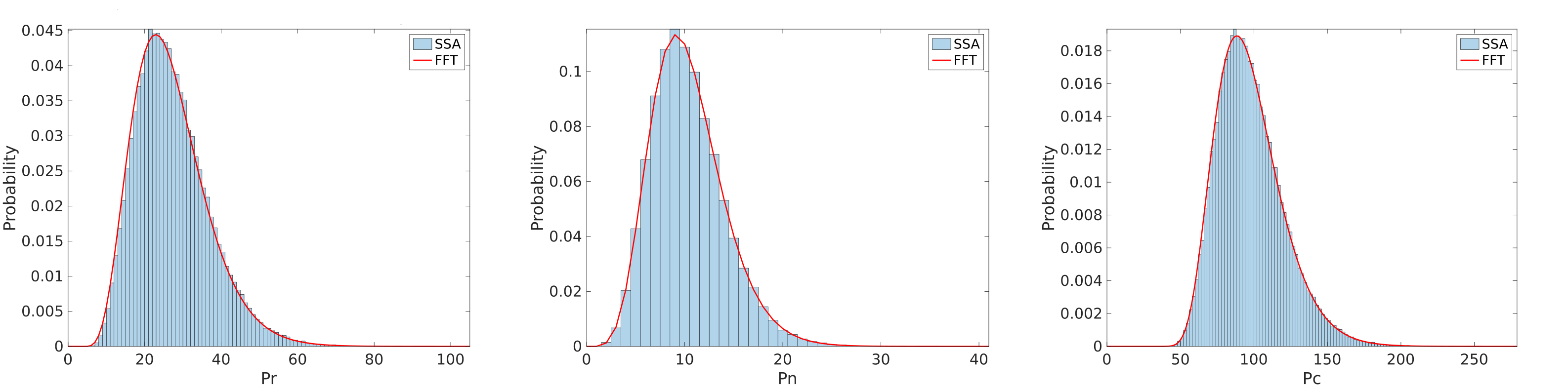
Figure 1. Comparison of marginal distributions calculated from FFT and Gillespie algorithm at $t=1500$. Left, ribosomes; middle, nuclear proteins; right, cytoplasmic proteins. System size $N=30$.

3.2.1. Gillespie algorithm

The Gillespie algorithm, or stochastic simulation algorithm (SSA) [17, 18], is one of the most widely-used numerical methods for CMEs, and here the histograms generated by the SSA are used as a benchmark for evaluating the other methods.

The major advantage of the SSA is that it works for larger system sizes (N$\sim$ $10^{5}$ to $10^{6}$) and long time spans ($t\geqslant 3000$s for $k_{t}=0.005$). Although the simulations can be time consuming when $N$ is large, the SSA may be parallelized to accelerate the simulations.

However, instead of calculating the distribution functions, the SSA only samples the underlying distribution. To obtain a true numerical solution of the CME (6), we therefore require other methods.

3.2.2. FFT method

Comparing the marginal distribution functions obtained from the FFT method and the histograms generated by the SSA (Fig. 1), we see that the FFT method works reliably for the CME (6) with deterministic initial conditions. Therefore, when it is tractable to use, the FFT method is our preferred the method for calculating the joint distributions used for the $NC_{cell}$ ratio curves.

However, due to the memory space limitation mentioned before, the FFT method only works for relatively small system sizes and short timespans. For example, on a computer with 16GB RAM, the FFT method will not run into memory space issues if the system size $N\sim 10^{2}$ and the time span $t\leqslant 3000$s. Although it would be possible to test the FFT method on computing clusters with much larger memory space, the aforementioned range of system size and timespan is already enough for the purpose of this paper.

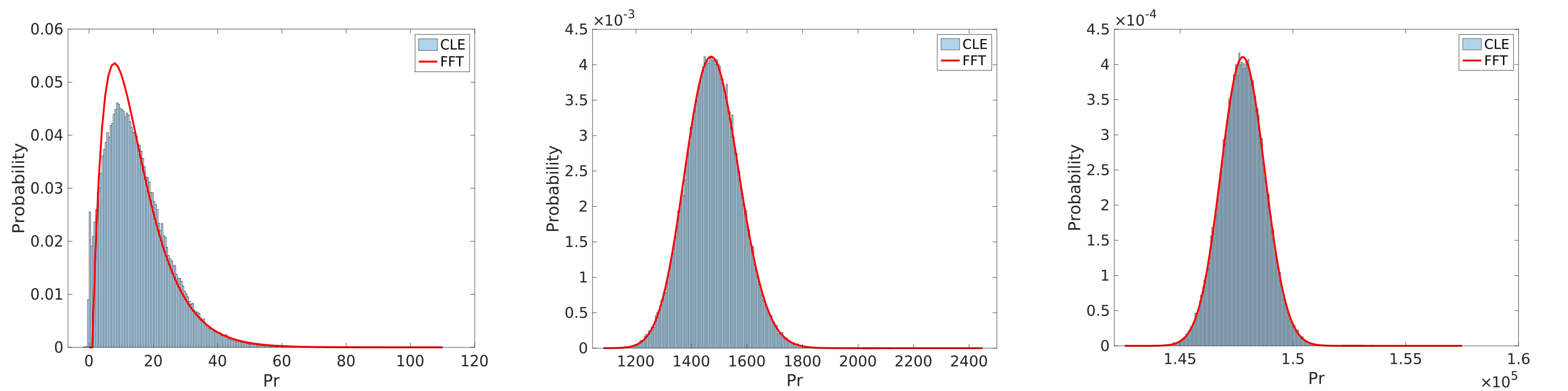
Figure 2. Comparison of marginal distributions of ribosome numbers calculated from FFT and CLE, with different system sizes. Left, $N=10^{1}$; middle, $N=10^{3}$; right, $N=10^{5}$.

3.2.3. Chemical Langevin equation approximation

We have shown in 2.1.3 that solving the CME (6) using the Fourier transform is a memory intensive process, especially when the system size variable $N$ increases and the number of grid points increases correspondingly. For biologically realistic values of $N$ with an order of magnitude of at least $10^{4}$, the Fourier transform method becomes numerically impractical, and approximation methods are needed to obtain the probability distributions from the CME (6). The chemical Langevin equation (CLE) is a widely-used method for large system size approximation, which can be derived by, e.g. the Kramers-Moyal expansion [16, 38], or continuous time Markov chain models for chemical reactions [1, 2].

The CLEs corresponding to the simplified translation model (5) are given by

(42a) $$dp_{r} =k_{r}p_{r}dt+\sqrt{k_{r}p_{r}}dW_{r}(t),$$

(42b) $$dp_{n} =k_{n}p_{r}dt+\sqrt{k_{n}p_{r}}dW_{n}(t),$$

(42c) $$dp_{c} =k_{c}p_{r}dt+\sqrt{k_{c}p_{r}}dW_{c}(t),$$

where $W_{l}(t)$ are independent standard Brownian motions, $l=r,n,c$. Now (42) is a system of stochastic differential equations, which can be solved numerically using, e.g. Euler-Maruyama method [19]. Then, the probability distributions can be obtained by generating a large enough number of sample paths from (42).

Fig. 2 shows a comparison of marginal distributions calculated from the FFT method and the CLE approximation. Here, we are using the marginal distribution of ribosome numbers as an example. We see that the CLE approximation does not work well when the system size variable $N$ is small, that is, when $N\sim 10^{1}$, and that the CLE approximation performs better as $N$ increases. When $N\sim 10^{5}$, the distributions calculated from FFT and CLE are nearly identical. Therefore, the CLE approximation is a valid method for simulations with large system sizes, e.g. simulations where $N\sim 10^{7}$ to $10^{8}$ for which the SSA becomes numerically impractical.

3.3. N/C ratio curves from the FFT method

Next we present the main results on the $NC_{cell}$ ratio curves calculated from the FFT method with deterministic initial conditions. We assume that for a particular cell immediately after cell division, the initial condition for the number of intracellular proteins is deterministic. In other words, Poisson or other stochastic initial conditions will only be relevant in the case of an ensemble of cells. For the $NC_{cell}$ ratio of a single cell, it therefore suffices to consider deterministic initial conditions.

3.3.1. Maintaining homeostasis of the N/C ratio via growth

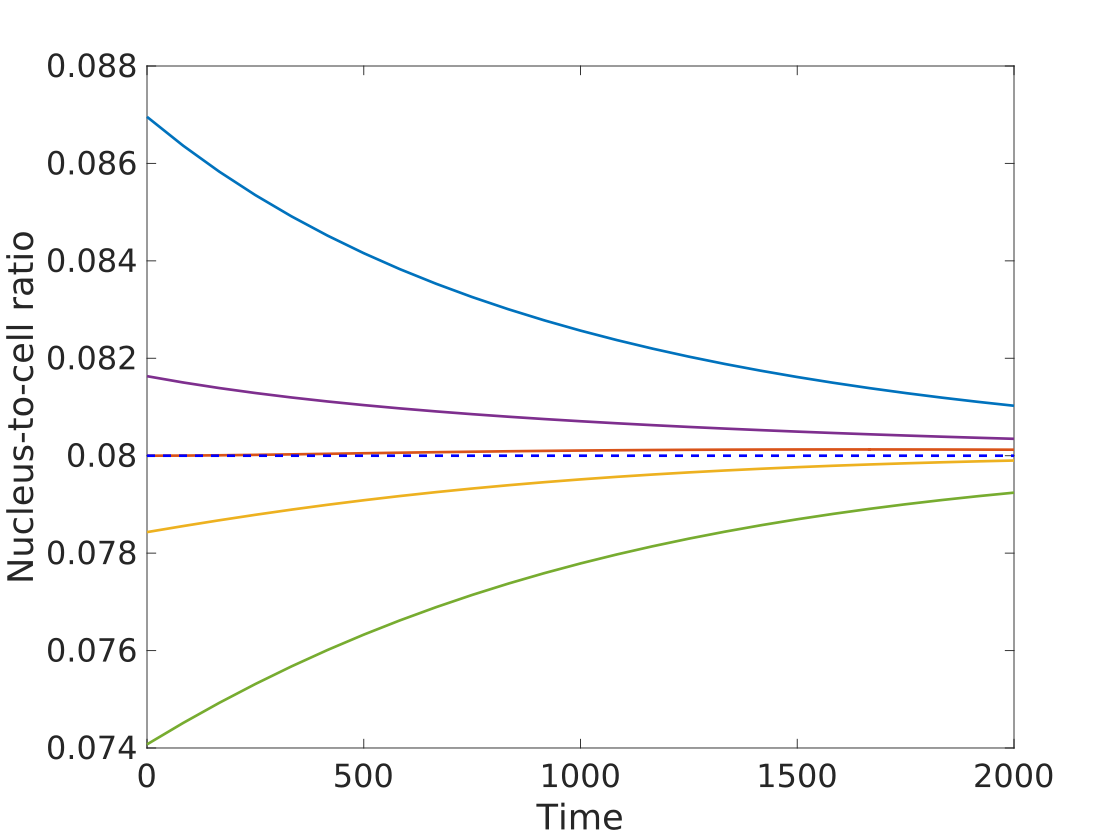
Figure 3. Mean nuclear-to-cell ratio curves with different initial conditions, showing relaxation to the steady-state value. System size $N=100$.

Fig. 3 shows that the mean $NC_{cell}$ ratio curves eventually approach $\phi_{n}=0.08$ if the initial ratio $NC_{cell,0}$ deviates from $\phi_{n}$. In other words, for this simplified translation model in which the protein numbers $p_{r}$, $p_{n}$, $p_{c}$ grow exponentially without bound, although the protein numbers themselves do not have steady states (other than the trivial steady state at 0), the ratio $NC_{cell}=\dfrac{p_{n}}{p_{r}+p_{n}+p_{c}}$ does approach the steady state $\phi_{n}$.

Interestingly, if the initial $NC_{cell}$ ratio is exactly equal to $\phi_{n}$, then due to fluctuations, the mean $NC_{cell}$ ratio curve may overshoot the steady state $\phi_{n}$. This overshot phenomenon diminishes as the system size variable $N$ increases, as will be shown later in the discussion of Taylor expansion approximation of the $NC_{cell}$ ratio.

Fig. 3 also shows that the more the initial ratio $NC_{cell,0}$ deviates from $\phi_{n}$, the faster the mean $NC_{cell}$ ratio will return to $\phi_{n}$, in the sense that there is a larger absolute value of the rate of change at any given time. It is worth noting that this behavior is achieved without any active feedback mechanism in the model, in agreement with our previous deterministic growth model [27].

3.3.2. Fluctuations of the N/C ratio and system size

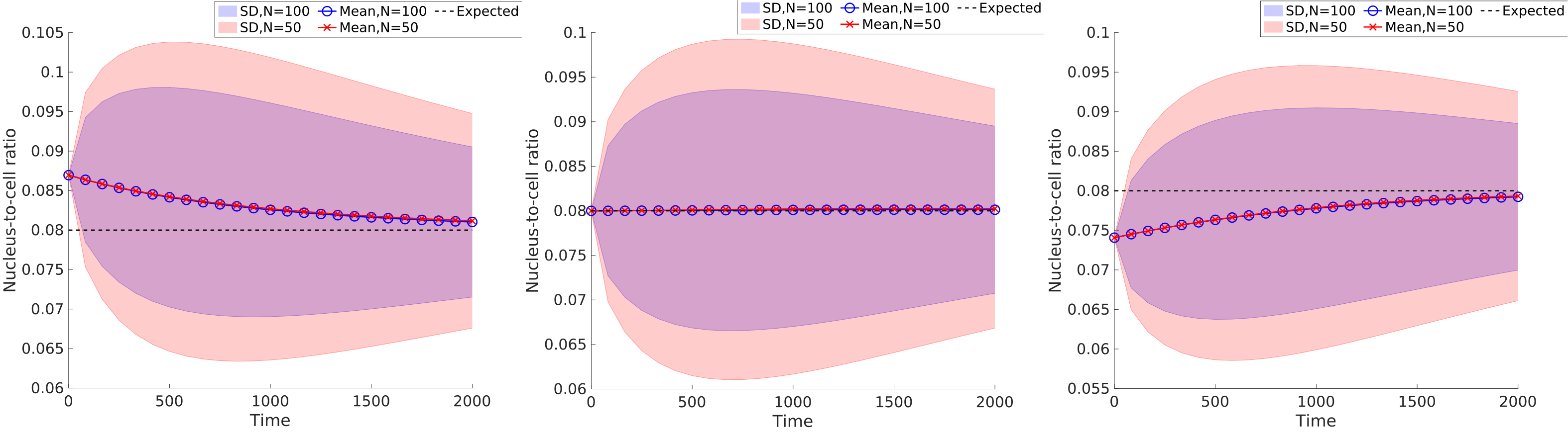
Figure 4. Nuclear-to-cell ratio curves with different initial conditions and system sizes.

Fig. 4 shows that the standard deviations of the $NC_{cell}$ ratio curves decrease as the system size $N$ increases. We will study the how the system size affects the magnitude of fluctuations in the $NC_{cell}$ ratio next in more detail.

3.4. N/C ratio curves from Taylor expansion approximation

Now we present the results on the $NC_{cell}$ ratio curves calculated from the Taylor expansion approximation.

3.4.1. Validity of Taylor expansion approximation

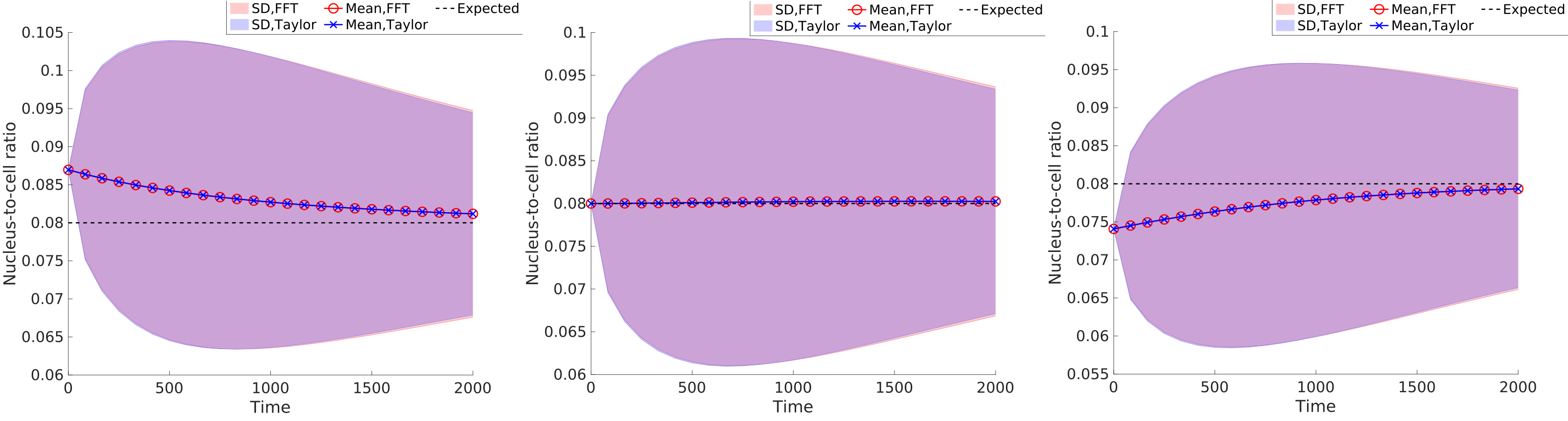
Figure 5. Nuclear-to-cell ratio curves calculated from FFT and Taylor expansion.

Fig. 5 shows examples of mean $NC_{cell}$ ratio curves and the corresponding standard deviations obtained from both the FFT method and the Taylor expansion approximation. We see that for a given initial condition, the mean $NC_{cell}$ ratio curves obtained by the two methods are nearly identical, while the standard deviations show small but noticeable difference. This comparison demonstrates that the Taylor expansion approximation agrees with the $NC_{cell}$ ratio calculated by the FFT method.

3.4.2. Expressions of Taylor series expansion approximations

Using the closed-form expressions of the means and variances of $p_{r}$, $p_{n}$, and $p_{c}$, we obtain explicit expressions of the Taylor series expansion approximation of the mean and variance of the $NC_{cell}$ ratio. Because these expressions in their explicit forms are quite technical, we present the results in a more concise form, which conveys the important information in a clearer way.

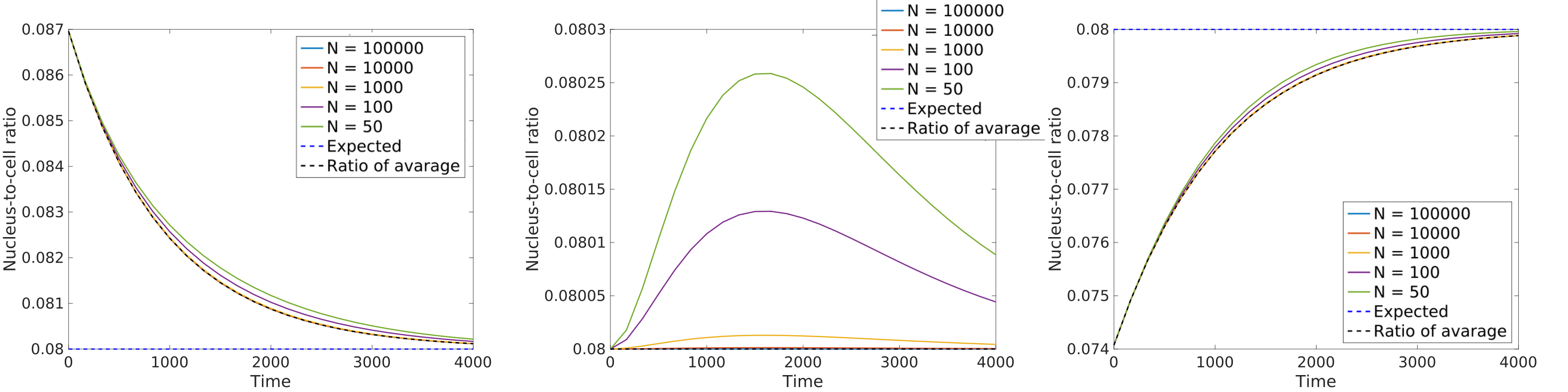
Figure 6. Nuclear-to-cell ratio curves with different initial conditions and system sizes, calculated from Taylor expansion.

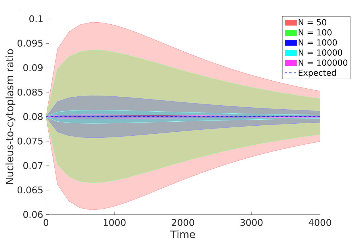
Figure 7. Standard deviation of the nuclear-to-cell ratio curve with different system sizes and initial condition $\phi_{n}=0.08$, calculated from Taylor expansion.

The expression for the mean of $NC_{cell}$ has the form

(43) $$\langle NC_{cell}\rangle =\left\langle\frac{p_{n}}{p_{r}+p_{n}+p_{c}}\right\rangle$$

$$\approx\frac{f_{n}\phi_{r}-f_{r}\phi_{n}+f_{r}\phi_{n}{e}^{k_{t}\phi_{r}t}}{f_{c}\phi_{r}+f_{n}\phi_{r}-f_{r}\phi_{c}-f_{r}\phi_{n}+f_{r}{e}^{k_{t}\phi_{r}t}}+\frac{F(k_{t},\phi_{r},\phi_{n},\phi_{c},f_{r},f_{n},f_{c},t)}{N}$$

$$=\frac{\langle p_{n}\rangle}{\langle p_{r}+p_{n}+p_{c}\rangle}+\frac{F_{M}(k_{t},\phi_{r},\phi_{n},\phi_{c},f_{r},f_{n},f_{c},t)}{N}.$$

As the system size $N\to\infty$, the terms that depend on $N$ in (43) go to zero, and we have

(44) $$\langle NC_{cell}(t)\rangle\to\frac{f_{n}\phi_{r}-f_{r}\phi_{n}+f_{r}\phi_{n}{e}^{k_{t}\phi_{r}t}}{f_{c}\phi_{r}+f_{n}\phi_{r}-f_{r}\phi_{c}-f_{r}\phi_{n}+f_{r}{e}^{k_{t}\phi_{r}t}}=\frac{\langle p_{n}(t)\rangle}{\langle p_{r}(t)\rangle+\langle p_{n}(t)\rangle+\langle p_{c}(t)\rangle},\quad N\to\infty.$$

In other words, as the system size increase, the mean of the ratio approaches the ratio of the mean (Fig. 6).

The expressions for the variances of $NC_{cell}$ has the form

(45) $$\mathrm{Var}(NC_{cell})=\frac{\langle p_{n}\rangle^{2}}{\langle p_{r}+p_{n}+p_{c}\rangle^{2}}\cdot\frac{F_{V}(k_{t},\phi_{r},\phi_{n},\phi_{c},f_{r},f_{n},f_{c},t)}{N},$$

so $\mathrm{Var}(NC_{cell})\to 0$, $N\to\infty$. That is, fluctuations of the $NC_{cell}$ ratio become negligible for sufficiently large values of the system size $N$ (Fig. 7).

3.5. N/C ratio fluctuation and cell division

We next study the effects of cell division on the homeostasis of the $NC_{cell}$ ratio. When cells divide, molecules and organelles are randomly segregated and distributed into the two daughter cells. A simple model of this random partitioning assumes that each molecule or organelle has a 50/50 chance to enter either of the two daughter cells, which then leads to binomial distributions. In reality, the segregation mechanisms are more complex, which would give rise to various degrees of randomness in the resulting distribution [21].

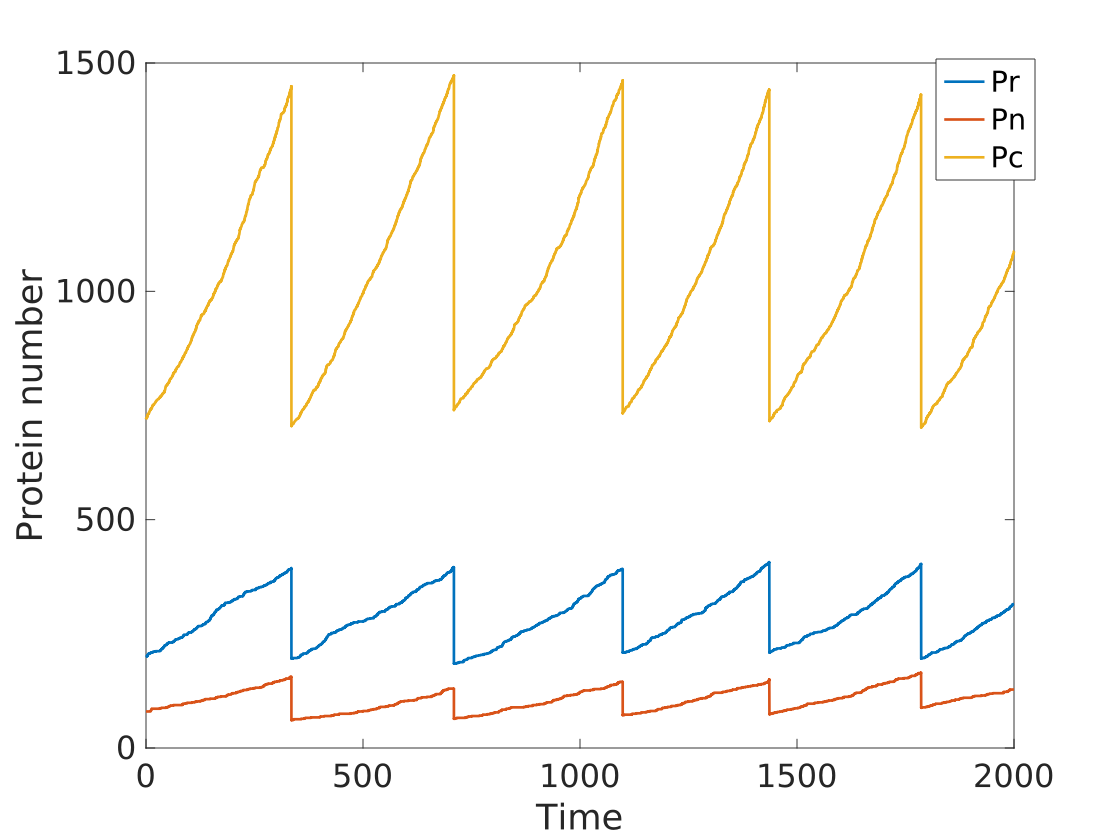
Figure 8. Sample protein number curves with 5 divisions. System size $N=1000$.

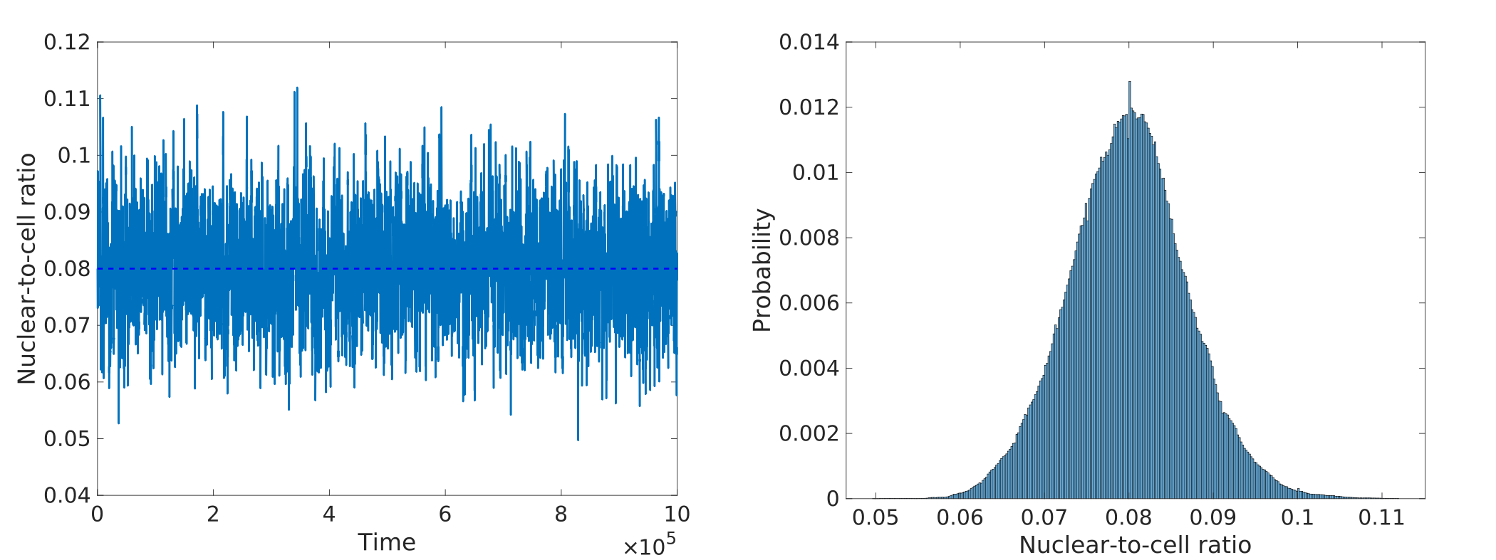
Figure 9. Left: sample $NC_{cell}$ ratio curve with 2870 divisions. Right: corresponding histogram of the $NC_{cell}$ ratio. System size $N=1000$.

Incorporating this simple model of cell division into the translation model is straightforward when using Gillespie algorithm for simulation. For instance, we may set a threshold for cell division by keeping track of an “initiator” protein corresponding to the DNA replication process [28]. Alternatively, we may specify a protein doubling division criterion by simply assuming that division occurs when the total number of proteins reaches twice the initial number. That is, the cell will divide whenever $p_{r}+p_{n}+p_{c}\geqslant 2(p_{r,0}+p_{n,0}+p_{c,0})$. After division, we track one of the daughter cells and set new initial values of protein numbers from binomial distributions based on the protein numbers at division. Fig. 8 shows sample curves of protein numbers from the protein doubling model with 5 divisions, and Fig. 9 shows a sample $NC_{cell}$ ratio curve and the corresponding histogram with 2870 divisions. We conjecture that as the number of divisions becomes large, the probability distribution of the $NC_{cell}$ ratio will approach a stable distribution, but further study is needed to reach a definite conclusion.

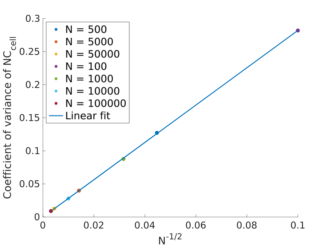
Figure 10. Plot of the coefficient of variance of the $NC_{cell}$ ratio as a function of the inverse square root of the system size variable $N$.

We observe that as the system size variable $N$ becomes large, the relative fluctuations in the $NC_{cell}$ ratio becomes smaller, even in the presence of extrinsic noises from cell division. We next examine $\mathrm{CV}(NC_{cell})$, the coefficient of variance of the $NC_{cell}$ ratio, as a function of $N^{-\frac{1}{2}}$, where

$$\mathrm{CV}(NC_{cell})=\frac{\mathrm{SD}(NC_{cell})}{\langle NC_{cell}\rangle}=\frac{\sqrt{\mathrm{Var}(NC_{cell})}}{\langle NC_{cell}\rangle},$$

and the mean $\langle NC_{cell}\rangle$ and variance $\mathrm{Var}(NC_{cell})$ are taken from all the data points in one SSA sample path, as is shown in Fig. 9. The result (Fig. 10) indeed shows that $\mathrm{CV}(NC_{cell})$ decreases as $N$ increases; moreover, the relationship between $\mathrm{CV}(NC_{cell})$ and $N^{-\frac{1}{2}}$ is linear, a sign that the law of large number holds for this simple growth-division model. This means that fluctuations of the $NC_{cell}$ ratio become negligible when the system size $N$ becomes large despite the extrinsic noises from cell division.

4. Discussion

Our simplified gene translation model, built upon our previous deterministic growth model [27], successfully demonstrates that the N/C ratio homeostasis is maintained when the stochasticity in cell growth is taken into account. This result holds in the case of unrestricted growth, which is clearly not biologically realistic due to resource limitations, as well as for a simple model of cell division, which we briefly explored in 3.5.

It is estimated that the order of magnitude of the typical concentration of proteins in cells is $10^{-1}$mM$\sim$1mM [5, 35]. Assuming that the volumes of cells are on the order of $10^{2}$µm³ [27, 40], the total number of proteins in a cell is expected to be on the order of $10^{7}\sim 10^{8}$. Our Taylor expansion approximation of the N/C ratio then shows that for this order of magnitude of proteins, the fluctuations in the N/C ratio are expected to be negligible. However, we have observed in our previous experiments that the N/C ratio does fluctuate in time (Figure 7C in [27]), although it is unclear to what extent these fluctuations are caused by measurement errors. Below we will discuss a number of possible sources of fluctuations in the N/C ratio which are not included in the current simplified model, and which may be the topic of future research.

It was shown in a previous stochastic growth model that the dynamics of mRNAs in the transcription process may be a major source of growth rate fluctuations [37]. However, in order to make the CME analytically solvable, we have removed transcription from the model entirely by assuming the translation rates are directly proportional to the gene fractions, thereby omitting this source of fluctuations.

In [37], transcription is modeled by a zeroth order reaction; whereas translation is modeled by a Michaelis-Menten kinetics for the ribosomes. Combining this model and the model in [28] which our current model is based on yields a transcription-translation model that assumes Michaelis-Menten kinetics for both the RNAPs and the ribosomes:

(46) $$P_{p}+G_{i}\ext@arrow 9999{\arrowfill@\leftarrow\relbar\rightarrow}{k_{g,i}^{-}}{k_{g,i}^{+}}C_{g,i},\quad C_{g,i}\xrightarrow{k_{0}}P_{p}+G_{i}+M_{i},\quad i=p,r,n,c\quad\mbox{(transcription);}$$

(47) $$P_{r}+M_{i}\ext@arrow 9999{\arrowfill@\leftarrow\relbar\rightarrow}{k_{m,i}^{-}}{k_{m,i}^{+}}C_{m,i},\quad C_{m,i}\xrightarrow{k_{t}}P_{r}+M_{i}+P_{i},\quad i=p,r,n,c\quad\mbox{(translation);}$$

(48) $$M_{i}\xrightarrow{\frac{1}{\tau}}\emptyset,\quad i=p,r,n,c\quad\mbox{(mRNA degredation).}$$

It can be shown [22] that if

1. the binding rate constants are identical for all genes, i.e.

   $$k_{g,i}^{+}=k_{g}^{+},\,k_{g,i}^{-}=k_{g}^{-},\,k_{m,i}^{+}=k_{m}^{+},\,k_{m,i}^{-}=k_{m}^{-};$$

2. the forward rate constants are large enough, i.e. $k_{g}^{+},k_{m}^{+}\to\infty$,

then at steady state, the average numbers of the enzyme-substrate complexes $c_{g,i}$ and $c_{m,i}$ will be

(49) $$\langle c_{g,i}\rangle=\frac{\langle g_{i}\rangle\langle p_{p,total}\rangle}{\sum\langle g_{i}\rangle}\quad\mbox{and}\quad\langle c_{m,i}\rangle=\frac{\langle m_{i}\rangle\langle p_{r,total}\rangle}{\sum\langle m_{i}\rangle},$$

where $p_{p,total}$ and $p_{r,total}$ are the total number of RNAPs and ribosomes, respectively. In this case, the Michaelis-Menten model is essentially equivalent to the model in [28]. Note, however, that in reality the above two assumptions may not hold. For example, in [4] the authors show that in E. coli the promotor on rates, which correspond to $k_{g,i}^{+}k_{0}$ in our Michaelis-Menten model, span more than three orders of magnitudes across genes, and are modulated by the cells to regulate gene expression. Therefore, it is unlikely the Michaelis-Menten model would be equivalent to the model in [28].

Besides including the fluctuations arising from transcription, this Michaelis-Menten model may reveal other possible sources of fluctuations in the N/C ratio as well. According to [20], the marginal distributions in reactions described by the Michaelis-Menten mechanism may become bimodal at intermediate times. In such cases, the coefficients of variation may no longer be of order $N^{-\frac{1}{2}}$ and fluctuations in protein numbers may still be prominent even if the system size gets large.

In our current model, the N/C ratio is calculated by simply calculating the ratio of nuclear and cytoplasmic protein numbers. In reality, nuclear proteins are translated in the cytoplasm and then imported into the nucleus through the nucleocytoplasmic transport process [40]. It is shown in [41] that nucleocytoplasmic transport plays an important role in the N/C ratio. While the nucleocytoplasmic transport has been studied extensively using both deterministic models (e.g. [24], [40]) and stochastical models (e.g. [30]), whether or not this transport process has significant contribution to the fluctuations in the N/C ratio is still unknown.

The random partioning of nuclear and cytoplasmic proteins at cell division may be yet another source of fluctuations in the N/C ratio for cells that are actively dividing. We have shown that in a simple growth-division model where the partitioning of molecules follow a binomial distribution with probability $1/2$, the fluctuations in the N/C ratio become negligible as the system size becomes sufficiently large. However, more complicated partioning mechanisms may lead to significant fluctuations in the N/C ratio. In particular, if the proteins are not independently partitioned at cell division but are partitioned into large clusters instead [21], then the induced fluctuation may be non-negligible even if the system size is large.

There are other potential sources of fluctuations in the $NC_{cell}$ ratio. For example, in [6] the authors hypothesized that fluctuations in cell volume may originate from biophysical sources, such as membrane tension and osmotic pressure. Admittedly, biochemical and biophysical processes in live cells are far more complicated than what our simplified gene translation model has encompassed. We believe that this simple model provides a foundation for future work on more realistic stochastic models of N/C ratio determination mechanisms.

References

- [1] David F Anderson and Thomas G Kurtz “Continuous time Markov chain models for chemical reaction networks” In Design and analysis of biomolecular circuits: engineering approaches to systems and synthetic biology Springer, 2011, pp. 3–42
- [2] David F Anderson and Thomas G Kurtz “Stochastic analysis of biochemical systems” Springer, 2015
- [3] Shruthi Balachandra, Sharanya Sarkar and Amanda A Amodeo “The Nuclear-to-Cytoplasmic Ratio: Coupling DNA Content to Cell Size, Cell Cycle, and Biosynthetic Capacity” In Annual Review of Genetics 56 Annual Reviews, 2022
- [4] Rohan Balakrishnan, Matteo Mori, Igor Segota, Zhongge Zhang, Ruedi Aebersold, Christina Ludwig and Terence Hwa “Principles of gene regulation quantitatively connect DNA to RNA and proteins in bacteria” In Science 378.6624 American Association for the Advancement of Science, 2022, pp. eabk2066
- [5] Abin Biswas, Omar Munoz, Kyoohyun Kim, Carsten Hoege, Benjamin M Lorton, David Shechter, Jochen Guck, Vasily Zaburdaev and Simone Reber “Conserved nucleocytoplasmic density homeostasis drives cellular organization across eukaryotes” In bioRxiv Cold Spring Harbor Laboratory, 2023, pp. 2023–09
- [6] Clotilde Cadart, Larisa Venkova, Matthieu Piel and Marco Cosentino Lagomarsino “Volume growth in animal cells is cell cycle dependent and shows additive fluctuations” In Elife 11 eLife Sciences Publications Limited, 2022, pp. e70816
- [7] Helena Cantwell and Paul Nurse “A homeostatic mechanism rapidly corrects aberrant nucleocytoplasmic ratios maintaining nuclear size in fission yeast” In Journal of Cell Science 132.22 The Company of Biologists Ltd, 2019, pp. jcs235911
- [8] Jeffrey Colgren and Pawel Burkhardt “Evolution: Was the nuclear-to-cytoplasmic ratio a key factor in the origin of animal multicellularity?” In Current Biology 33.8 Elsevier, 2023, pp. R298–R300
- [9] Edwin Grant Conklin “Cell size and nuclear size” Princeton University Press, 1914
- [10] Max Delbrück “Statistical fluctuations in autocatalytic reactions” In The journal of chemical physics 8.1 American Institute of Physics, 1940, pp. 120–124
- [11] Dan Deviri and Samuel A Safran “Balance of osmotic pressures determines the nuclear-to-cytoplasmic volume ratio of the cell” In Proceedings of the National Academy of Sciences 119.21 National Acad Sciences, 2022, pp. e2118301119
- [12] Regina C Elandt-Johnson and Norman L Johnson “Survival models and data analysis” John Wiley & Sons, 1980
- [13] Stefan Engblom “A discrete spectral method for the chemical master equation” In Technical Report 2006-036, 2006
- [14] Stefan Engblom “Galerkin spectral method applied to the chemical master equation” In Commun. Comput. Phys 5.5, 2009, pp. 871–896
- [15] Stefan Engblom “Spectral approximation of solutions to the chemical master equation” In Journal of computational and applied mathematics 229.1 Elsevier, 2009, pp. 208–221
- [16] Crispin W Gardiner “Handbook of stochastic methods” springer Berlin, 1985
- [17] Daniel T Gillespie “A general method for numerically simulating the stochastic time evolution of coupled chemical reactions” In Journal of computational physics 22.4 Elsevier, 1976, pp. 403–434
- [18] Daniel T Gillespie “Exact stochastic simulation of coupled chemical reactions” In The journal of physical chemistry 81.25 ACS Publications, 1977, pp. 2340–2361
- [19] Desmond J Higham “An algorithmic introduction to numerical simulation of stochastic differential equations” In SIAM review 43.3 SIAM, 2001, pp. 525–546
- [20] James Holehouse, Augustinas Sukys and Ramon Grima “Stochastic time-dependent enzyme kinetics: Closed-form solution and transient bimodality” In The Journal of Chemical Physics 153.16 AIP Publishing, 2020
- [21] Dann Huh and Johan Paulsson “Random partitioning of molecules at cell division” In Proceedings of the National Academy of Sciences 108.36 National Acad Sciences, 2011, pp. 15004–15009
- [22] CJ Jachimowski, DA McQuarrie and ME Russell “A stochastic approach to enzyme-substrate reactions” In Biochemistry 3.11 ACS Publications, 1964, pp. 1732–1736
- [23] Tobias Jahnke and Wilhelm Huisinga “Solving the chemical master equation for monomolecular reaction systems analytically” In Journal of mathematical biology 54 Springer, 2007, pp. 1–26
- [24] Sanghyun Kim and Michael Elbaum “A simple kinetic model with explicit predictions for nuclear transport” In Biophysical journal 105.3 Elsevier, 2013, pp. 565–569
- [25] Ian J Laurenzi “An analytical solution of the stochastic master equation for reversible bimolecular reaction kinetics” In The Journal of Chemical Physics 113.8 American Institute of Physics, 2000, pp. 3315–3322
- [26] Chang Hyeong Lee and Pilwon Kim “An analytical approach to solutions of master equations for stochastic nonlinear reactions” In Journal of Mathematical Chemistry 50 Springer, 2012, pp. 1550–1569
- [27] Joël Lemière, Paula Real-Calderon, Liam J Holt, Thomas G Fai and Fred Chang “Control of nuclear size by osmotic forces in Schizosaccharomyces pombe” In Elife 11 eLife Sciences Publications Limited, 2022, pp. e76075
- [28] Jie Lin and Ariel Amir “Homeostasis of protein and mRNA concentrations in growing cells” In Nature communications 9.1 Nature Publishing Group UK London, 2018, pp. 4496
- [29] Michael J Moore, Joseph A Sebastian and Michael C Kolios “Determination of cell nucleus-to-cytoplasmic ratio using imaging flow cytometry and a combined ultrasound and photoacoustic technique: a comparison study” In Journal of Biomedical Optics 24.10 Society of Photo-Optical Instrumentation Engineers, 2019, pp. 106502–106502
- [30] Ruhollah Moussavi-Baygi, Yousef Jamali, Reza Karimi and Mohammad RK Mofrad “Brownian dynamics simulation of nucleocytoplasmic transport: a coarse-grained model for the functional state of the nuclear pore complex” In PLoS computational biology 7.6 Public Library of Science San Francisco, USA, 2011, pp. e1002049
- [31] Brian Munsky and Mustafa Khammash “The finite state projection algorithm for the solution of the chemical master equation” In The Journal of chemical physics 124.4 AIP Publishing, 2006
- [32] Frank R Neumann and Paul Nurse “Nuclear size control in fission yeast” In The Journal of cell biology 179.4 Rockefeller University Press, 2007, pp. 593–600
- [33] Marine Olivetta and Omaya Dudin “The nuclear-to-cytoplasmic ratio drives cellularization in the close animal relative Sphaeroforma arctica” In Current Biology 33.8 Elsevier, 2023, pp. 1597–1605
- [34] Matthias Reis, Justus A Kromer and Edda Klipp “General solution of the chemical master equation and modality of marginal distributions for hierarchic first-order reaction networks” In Journal of mathematical biology 77 Springer, 2018, pp. 377–419
- [35] Romain Rollin, Jean-Francois Joanny and Pierre Sens “Cell size scaling laws: a unified theory” In bioRxiv Cold Spring Harbor Laboratory, 2022
- [36] Sahla Syed, Henry Wilky, João Raimundo, Bomyi Lim and Amanda A Amodeo “The nuclear to cytoplasmic ratio directly regulates zygotic transcription in Drosophila through multiple modalities” In Proceedings of the National Academy of Sciences 118.14 National Acad Sciences, 2021, pp. e2010210118
- [37] Philipp Thomas, Guillaume Terradot, Vincent Danos and Andrea Y Weiße “Sources, propagation and consequences of stochasticity in cellular growth” In Nature communications 9.1 Nature Publishing Group UK London, 2018, pp. 4528
- [38] Nicolaas Godfried Van Kampen “Stochastic processes in physics and chemistry” Elsevier, 1992
- [39] John J Vastola “Solving the chemical master equation for monomolecular reaction systems and beyond: a Doi-Peliti path integral view” In Journal of Mathematical Biology 83.5 Springer, 2021, pp. 48
- [40] Ching-Hao Wang, Pankaj Mehta and Michael Elbaum “Thermodynamic paradigm for solution demixing inspired by nuclear transport in living cells” In Physical review letters 118.15 APS, 2017, pp. 158101
- [41] Yufei Wu, Adrian F Pegoraro, David A Weitz, Paul Janmey and Sean X Sun “The correlation between cell and nucleus size is explained by an eukaryotic cell growth model” In PLOS Computational Biology 18.2 Public Library of Science San Francisco, CA USA, 2022, pp. e1009400