A phase field model for deformation-induced amorphization

Abstract

Amorphization by severe plastic deformation has been observed in various crystalline materials. However, developing a quantitative and comprehensive theory for strain-induced amorphization remains challenging due to the complex nature of microstructural evolutions and deformation mechanisms. We propose a phase field model coupled with elastic-plastic theory to study the strain-induced amorphization in nanocrystalline materials. The plastic behaviors of crystalline phases and amorphous phases are coupled with phase evolutions by finite strain theory through the strain energy. This coupled model enables to quantitatively explore the effects of various defects on formation of amorphous phases such as shear bands. Simulations using our model predict that amorphous nucleation follows the martensitic transformation, and occurs primarily within localized regions of high stress, including shear bands. Our results also indicate an increase in the critical plastic strain for amorphization as the grain size increases. These findings align well with experimental results, validating the proposed model in capturing key features of deformation-induced amorphization. Our work provides valuable insights into deformation-induced amorphization and serves as a basis for developing more quantitative models with complex microscopic mechanisms.

1 Introduction

Amorphization processes have been commonly found in crystalline materials under various macroscale severe plastic deformation techniques, including cold rolling, ball milling, etc. [1, 2, 3, 4, 5, 6]. For instance, Waitz et al. [1] achieved nearly complete amorphization in bulk Ni–50.3at.%Ti by high-pressure torsion. Hua et al. [3] also found that the amorphization happened in the NiTi micropillars under serve shear deformation. Li et al. [6] reviewed amorphization under mechanical deformation and concluded that deformation introduces defects in the crystal structure, creating favorable conditions for amorphization. However, during dynamical deformation, complex microstructural evolutions, including phase evolutions like martensitic transformations and developments of defects such as shear bands, make it challenging to explore strain-induced amorphization quantitatively [5, 6]. Moreover, insufficient study on microstructural evolutions sometimes leads to conflicting explanations for the amorphous phase forming [3, 7, 5]. For example, Koike et al. [8] considered the amorphization process depending on dislocation accumulation, while Yamada and Koch [9] believed that amorphous phases directly grow at grain boundaries without dislocations. A comprehensive theory of strain-induced amorphization, which incorporates microstructure evolutions, remains elusive.

The deformation-induced amorphization is often related to nanocrystallization and phase evolutions in experiments [8, 2, 10, 11, 3]. Koike et al. [8] confirmed the coexistence of nanocrystalline and amorphous phases by observing sharp diffraction rings superimposed on an amorphous halo. Jiang et al. [10] viewed nanocrystalline phases as a transition from coarse grains to amorphous phases. Recently, the relation between amorphization and martensitic transformation also attracts much attention. Jiang et al. [2] proposed a sequence where the initial austenitic phase transforms into the martensitic phase, ultimately leading to the amorphous phase under local canning compression. Hua et al. [3] suggested a similar sequence of microstructure evolution preceding amorphization in nanocrystalline NiTi alloy. The uniaxial compression experiments on NiTi micropillars showed that the amorphization is initiated in the martensite instead of the austenite. Furthermore, Zhang et al. [11] established an explicit experimental link between martensitic transformations and solid-state amorphization for $\beta$-Ti alloy. These imply that the intrinsic connection between amorphization and martensitic transformations might help to reveal underlying mechanisms of strain-induced amorphization.

Some theories that have been successfully applied to martensitic transformations are promising to uncover mechanisms of amorphization, such as molecular dynamics and phase field approaches. Numerous studies have utilized molecular dynamics to explore amorphization phenomena induced by nanoindentation, high strain rates, and shear strain [6, 3, 12]. For example, using molecular dynamics, Fan et al. [12] investigated the amorphization process induced by the nanoindentation. The nanoindentation simulations demonstrated that grain boundaries contribute significantly to the amorphization. However, molecular dynamics primarily focuses on the atomic scale and performs simulations with high loading rates. Thus, insights into plasticity and the amorphization mechanism provided by atomic models are limited. On the other hand, phase field approaches offer a realistic framework for simulating thermodynamic and microstructural evolutions [13, 14, 15, 16]. For instance, Xu and Kang [13] proposed a two-dimensional phase field model for NiTi alloy considering martensitic transformations to investigate the super-elasticity, elastocacaloric effect, shape memory effect, etc. The numerical simulations revealed the complicated microstructure evolutions in the geometrically graded NiTi alloy. This demonstrated the broad applicability of phase field models. Specifically, phase variables change under different driving forces, including compositional gradients, temperature, and strain. It is also straightforward to quantitatively consider plastic behaviors of phases. Accordingly, phase field models have been widely employed in studying martensitic transformations, grain growth, twinning, etc. [17, 18, 19, 20, 21, 22, 23, 24, 25, 26, 27, 28, 29, 25]. However, phase field approaches have not yet been applied to investigate the evolution of the amorphous phase in highly deformed materials. Notably, phase field models are coupled with finite strain theory and extensively applied to investigate multiphase problems under severe deformation. Levitas [28] successfully applied the phase field theory at large strains to explore phase transformations in various materials under uniaxial loading. This is promising to use phase field approaches to uncover the deformation mechanisms that govern the formation and behavior of amorphous phases in large-deformed crystalline materials.

In this paper, we propose a novel phase field model to study the amorphization process in highly-deformed crystalline materials. Two phase variables are used to describe martensitic transformations and amorphization. Martensitic transformations are driven by the free energy difference between the martensite and the austenite, while the amorphization is actuated by the strain energy from severe deformations. By combining the phase field model with finite strain theory, we quantitatively consider the plasticity and evolution of crystalline and amorphous phases, capturing intricate interplay between severe mechanical deformation and amorphization. The coupled model allows for consideration of the evolution of various defects in strain-induced amorphization, including shear bands, grain boundaries, and dislocations. The proposed model provides a comprehensive framework for quantitatively studying deformation-induced amorphization under various microscopic mechanisms.

We perform numerical simulations using our model on the nanocrystalline NiTi alloy under two-dimensional and three-dimensional settings. Simulation results show that an amorphous phase forms in the martensite and grows under severe deformations. The effect of the grain size on amorphization is investigated and simulation results demonstrate that the critical plastic strain for amorphization increases as the grain size increases. When shear bands are introduced in simulations, the amorphous phase nucleates primarily within shear bands, indicating that highly distorted regions facilitate favorable conditions for amorphous nucleation. These observations are in good agreement with various experimental findings reported in literature [3, 30, 31, 32]. These simulations validate the proposed phase field model in capturing the essential features of deformation-induced amorphization. They also provide valuable insights into the intrinsic mechanisms, enabling better understandings of deformation-induced amorphization. Our proposed phase field model serves as a basis for developing more quantitative theories related to strain-induced amorphization.

The paper is structured as follows: Section 2 introduces the proposed phase field model for amorphization coupled with finite strain theory. In Section 3, we present a linearized theory for efficient numerical simulations. Section 4 shows the applicability of our model through applications, including shear in two dimensions and compression in three dimensions. The effects of grain sizes and shear bands are also investigated. Finally, we provide a conclusion in Section 5.

2 Phase field model for amorphization

A phase-field approach is employed to capture the microstructural evolution during strain-induced amorphization. We start with the austenitic phase in our model. Upon loading, the parent phase transforms into the martensitic phase, eventually leads to the amorphous phase.

2.1 Order parameters

The phase field models for martensitic transformation consider a continuous field variable, $\eta_{M}\in[0,1]$, which specifies the martensite ($\eta_{M}=1$) and the austenite ($\eta_{M}=0$) in a given region [33, 34]. Under large deformation, the amorphous phase forms. We define another continuous field variable, $\eta_{g}\in[0,1]$, for the amorphous phase. Specifically, $\eta_{M}=\eta_{g}=0$ represents the austenitic phase, while $\eta_{M}=1,\eta_{g}=0$ defines the martensitic phase. The amorphous phase is characterized by $\eta_{M}=0,\eta_{g}=1$. Considering $\eta_{M}\leq 1$ in martensitic transformations, $\eta_{M}\leq 1-\eta_{g}$ is a straightforward generalization in the amorphization process, i.e.,

$$\eta_{M}+\eta_{g}\leq 1,$$ (1)

where $1-\eta_{M}-\eta_{g}$ represents the existence of the austenitic phase in a given region. These phase field variables, $\eta_{M}$ and $\eta_{g}$, also are named in order parameters.

2.2 Kinematics

We consider a reference configuration $\Omega_{0}\subset\mathbb{R}^{3}$ and a material point $\bm{x}$ within $\Omega_{0}$. The kinematics of finite deformation is described by a field $\mathcal{X}(\bm{x}):\bm{x}\in\Omega_{0}\rightarrow\bm{X}\in\Omega$, mapping point $\bm{x}$ to point $\bm{X}$ in the deformed configuration $\Omega$. The total deformation gradient, given by $\bm{F}=\frac{\partial\mathcal{X}}{\partial\bm{x}}$ is multiplicatively decomposed as [35]

$$\bm{F}=\bm{F}_{e}\bm{F}_{p},$$ (2)

where $\bm{F}_{e}$ is the elastic part of the deformation gradient, and the inelastic part, $\bm{F}_{p}$, accounts for contributions from crystalline and amorphous regions. The evolution rate of the plastic deformation gradient, i.e.,

$$\dot{\bm{F}}_{p}=\bm{L}_{p}\bm{F}_{p},$$ (3)

is determinied by the plastic velocity gradient $\bm{L}_{p}$. The plastic velocity gradient can be formulated as the sum of the shear rates on $N_{s}$ slip systems in crystal and the visco-plastic strain rate in the amorphous phase [36, 37]:

$$\bm{L}_{p}=\left(1-h(\eta_{g})\right)\sum_{\alpha=1}^{N_{s}}\dot{\gamma}^{\alpha}\bm{m}^{\alpha}\otimes\bm{n}^{\alpha}+h(\eta_{g})\bm{L}_{g}^{p},$$ (4)

where $\bm{L}_{g}^{p}$ is the plastic velocity gradient in amorphous regions, $\dot{\gamma}^{\alpha}$ is the shear rate on the slip system $\alpha$, and the vectors $\bm{m}^{\alpha}$ and $\bm{n}^{\alpha}$ indicate the slip direction and the slip plane normal, respectively. An interpolation function is used to represent the local phase volume fraction,

$$h(\eta)=2\eta^{2}-\eta^{4},$$ (5)

where $\eta$ can be $\eta_{M}$ and $\eta_{g}$, and $h(\eta)$ is the local volume fraction of a given phase.

The following plastic flow rule of crystalline phases is used. For the slip system $\alpha$, the shear rate reads [38, 39]

$$\dot{\gamma}^{\alpha}=\dot{\gamma}_{0}\left|\frac{\tau^{\alpha}}{\tau_{c}^{\alpha}}\right|^{\frac{1}{m}}sgn(\tau^{\alpha}),$$ (6)

where $\tau^{\alpha}$ is the resolved shear stress on the slip system $\alpha$. $\dot{\gamma}_{0}$ and $m$ are material parameters. $\tau_{c}^{\alpha}$ is the slip resistance on the slip system $\alpha$, which can be given by the hardening behavior:

$$\tau_{c}^{\alpha}=\sum_{\beta=1}^{N_{s}}h_{\alpha\beta}|\dot{\gamma}^{\beta}|,$$ (7)

in which $h_{\alpha\beta}$ is the hardening matrix, and the index $\beta$ is refered to slip systems.

Considering the plastic flow rule for amorphous, we define $\tau_{D,d}$ as the deviatoric Kirchhoff stress tensor, and then we get the visco-plastic flow vector is derived as [40, 41, 42, 43, 44]:

$$\bm{N}=\sqrt{\frac{1}{2}}\frac{\tau_{D,d}}{\|\tau_{D,d}\|},$$ (8)

where $\|\cdot\|$ denotes the Frobenius norm. The plastic velocity gradient for the amorphous phase can be formulated as

$$\bm{L}_{g}^{p}=\dot{\gamma}_{g}(\bm{R}_{e})^{T}\bm{N}\bm{R}_{e},$$ (9)

where $\dot{\gamma}_{g}$ denotes the visco-plastic multiplier and $\bm{N}$ is the visco-plastic flow vector. $\bm{R}_{e}$ is the elastic rotation tensor, satisfying $\bm{R}_{e}=\bm{F}_{e}\left[(\bm{F}_{e})^{T}\bm{F}_{e}\right]^{-\frac{1}{2}}$. Considering the visco-plastic multiplier, we define it as

$$\dot{\gamma}_{g}=\frac{1}{A}\sinh{\frac{\tau_{D}^{eq}}{\tau^{*}}},$$ (10)

where $A$ is an Eyring-related function, and we choose it as a material parameter to simplify models. $\tau_{D}^{eq}$ is a Kirchhoff equivalent stress defined as $\tau_{D}^{eq}=\sqrt{\frac{1}{2}}\|\tau_{D,d}\|$ and the material constant $\tau^{*}=\frac{2k_{B}T}{V_{\text{atom}}}$ is the reference stress. $V_{\text{atom}}$ is the atomic volume, $k_{B}$ is the Boltzmann constant and $T$ is the absolute temperature.

2.3 Free energy functional

The free energy functional of the system, $E$, consists of local phase separation energy $E_{local}$, the gradient energy $E_{grad}$ and the elastic strain energy $E_{el}$:

$$E\left(\eta_{M},\eta_{g},\bm{F}_{e}\right) =E_{local}\left(\eta_{M},\eta_{g}\right)+E_{grad}\left(\nabla\eta_{M},\nabla\eta_{g}\right)+E_{el}\left(\eta_{M},\eta_{g},\bm{F}_{e}\right),$$ (11)

$$=\int_{\Omega}\left[e_{local}\left(\eta_{M},\eta_{g}\right)+e_{grad}\left(\nabla\eta_{M},\nabla\eta_{g}\right)+e_{el}\left(\eta_{M},\eta_{g},\bm{F}_{e}\right)\right]d\bm{x},$$

where $\eta_{M}$ and $\eta_{g}$ are order parameters, and $\bm{F}_{e}$ represents the elastic deformation gradient. $e_{local}$, $e_{grad}$ and $e_{el}$ are energy densities related with $E_{local}$, $E_{grad}$ and $E_{el}$, respectively.

2.3.1 Local phase separation energy

The bulk thermodynamic properties of the system dominate the local phase separation energy density, $e_{local}$, which can be represented by a Landau-type polynomial:

$$e_{local}\left(\eta_{M},\eta_{g}\right) =\kappa_{M}\left(\frac{A_{M}}{2}\eta_{M}^{2}-\frac{B_{M}}{3}\eta_{M}^{3}+\frac{C_{M}}{4}\eta_{M}^{4}\right)$$ (12)

$$+\kappa_{g}\left(\frac{A_{g}}{2}\eta_{g}^{2}-\frac{B_{g}}{3}\eta_{g}^{3}+\frac{C_{g}}{4}\eta_{g}^{4}\right)+\kappa_{Mg}\frac{D}{2}\eta_{M}^{2}\eta_{g}^{2},$$

where the function has value of 0 at $\eta_{M}=\eta_{g}=0$, which corresponds to the austenite. The constants $A_{M},B_{M},C_{M},$ $A_{g},B_{g},C_{g},$ and $D$ determine the shape of the local phase separation energy. $\kappa_{M}$ represents the energy difference between austenite and martensite, while $\kappa_{g}$ denotes the energy gap between the amorphous and austenitic parent phases. $\kappa_{Mg}$ represents the barrier to the coexistence of martensite and amorphous phases. Based on the thermodynamics of martensitic transformation and amorphization, we know that the function value of the martensitic phase should be lower than that of the austenite. Besides this, the value of the amorphous phase is higher than that of the austenitic parent phase [6],

$$\frac{A_{M}}{2}-\frac{B_{M}}{3}+\frac{C_{M}}{4} \leq 0,$$ (13)

$$\frac{A_{g}}{2}-\frac{B_{g}}{3}+\frac{C_{g}}{4} \geq 0.$$

We also notice that the partial derivative of the local phase separation energy concerning the field variables should be zero when $\eta_{i}=0,\forall i\in\{M,g\}$ or $\eta_{i}=0,\eta_{j}=1$, for all $i\neq j\in\{M,g\}$, such that the pure phase corresponds to a local energy minimum. These requirements give constraints as follows:

$$A_{M}-B_{M}+C_{M} =0,$$ (14)

$$A_{g}-B_{g}+C_{g} =0.$$

Based on those constraints, we can choose suitable parameters for numerical simulations.

Considering the local phase separation energy, the driving force on each field variable associated with it reads:

$$f_{\eta_{M}}^{local} =-\frac{\delta e_{local}}{\delta\eta_{M}}$$ (15)

$$=-\kappa_{M}\left(A_{M}\eta_{M}-B_{M}\eta_{M}^{2}+C_{M}\eta_{M}^{3}\right)-\kappa_{Mg}D\eta_{M}\eta_{g}^{2},$$

$$f_{\eta_{g}}^{local} =-\frac{\delta e_{local}}{\delta\eta_{g}}$$

$$=-\kappa_{g}\left(A_{g}\eta_{g}-B_{g}\eta_{g}^{2}+C_{g}\eta_{g}^{3}\right)-\kappa_{Mg}D\eta_{M}^{2}\eta_{g}.$$

2.3.2 Gradient energy

The gradient energy defines the energy of the interface between various phases. We can express its density, $e_{grad}$, as follows:

$$e_{grad}\left(\nabla\eta_{M},\nabla\eta_{g}\right)=\frac{1}{2}\beta_{M}|\nabla\eta_{M}|^{2}+\frac{1}{2}\beta_{g}|\nabla\eta_{g}|^{2},$$ (16)

where $\beta_{M}$ and $\beta_{g}$ are coefficients related to the interfacial energy between neighboring phases.

The driving force on each field associated with $e_{local}$ can be given by:

$$f_{\eta_{M}}^{grad} =-\frac{\delta e_{grad}}{\delta\eta_{M}}=\beta_{M}\nabla^{2}\eta_{M},$$ (17)

$$f_{\eta_{g}}^{grad} =-\frac{\delta e_{grad}}{\delta\eta_{g}}=\beta_{g}\nabla^{2}\eta_{g}.$$

2.3.3 Strain energy

The elastic strain energy density can be written as,

$$e_{el}\left(\eta_{M},\eta_{g},\bm{F}_{e}\right)=\frac{1}{2}\bm{E}_{e}:\mathbb{C}(\eta_{M},\eta_{g}):\bm{E}_{e},$$ (18)

where $\bm{E}_{e}=\frac{1}{2}\left(\bm{F}_{e}^{T}\bm{F}_{e}-I\right)$ is the elastic strain tensor, and elastic coefficients in mixed regions are interpolated as follows,

$$\mathbb{C}\left(\eta_{M},\eta_{g}\right)=\mathbb{C}_{A}+[\mathbb{C}_{M}-\mathbb{C}_{A}][1-h(\eta_{g})]h(\eta_{M})+[\mathbb{C}_{g}-\mathbb{C}_{A}]h(\eta_{g}),$$ (19)

where $h(\eta)$ is the interpolation function (5). $\mathbb{C}_{A}$, $\mathbb{C}_{M}$, and $\mathbb{C}_{g}$ define the elastic coefficients matrix in austenite, martensite, and amorphous. $\eta_{M}=\eta_{g}=0$ defines the austenitic phase and the elastic constants give $\mathbb{C}=\mathbb{C}_{A}$. For the martensitic phase, $\eta_{M}=1,\eta_{g}=0$ shows $\mathbb{C}=\mathbb{C}_{M}$. $\eta_{M}=0,\eta_{g}=1$ gives $\mathbb{C}=\mathbb{C}_{g}$ for amorphous.

Following the variation method, the equilibrium equations can be given by:

$$\nabla\cdot\bm{P}=0,$$ (20)

where $\bm{P}$ is the first Piola-Kirchhoff stress tensor and it obeys $\bm{P}=\frac{\partial e_{el}}{\partial\bm{F}}$. It is not difficult to find that,

$$\bm{P}=\frac{\partial e_{el}}{\partial\bm{E}_{e}}:\frac{\partial\bm{E}_{e}}{\partial\bm{F}_{e}}:\frac{\partial\bm{F}_{e}}{\partial\bm{F}}=\bm{F}_{e}\left(\mathbb{C}:\bm{E}_{e}\right)\bm{F}_{p}^{-T},$$

where the plastic deformation gradient can be given by the plastic flow (3).

The driving force on each field variable associated with the elastic energy is:

$$f_{M}^{el} =-\frac{\partial e_{el}}{\partial\eta_{M}}=-\frac{1}{2}\bm{E}_{e}:\frac{\partial\mathbb{C}}{\partial\eta_{M}}:\bm{E}_{e},$$ (21)

$$f_{g}^{el} =-\frac{\partial e_{el}}{\partial\eta_{g}}=-\frac{1}{2}\bm{E}_{e}:\frac{\partial\mathbb{C}}{\partial\eta_{g}}:\bm{E}_{e}-\frac{\partial e_{el}}{\partial\bm{E}_{e}}:\frac{\partial\bm{E}_{e}}{\partial\eta_{g}},$$

where $\frac{\partial e_{el}}{\partial\bm{E}_{e}}=\mathbb{C}:\bm{E}_{e}$ is the elastic second Piola-Kirchhoff stress and $\frac{\partial\bm{E}_{e}}{\partial\eta_{g}}=\frac{\partial\bm{E}_{e}}{\partial\bm{F}_{e}}\frac{\partial\bm{F}_{e}}{\partial\bm{F}_{p}^{-1}}\frac{\partial\bm{F}_{p}^{-1}}{\partial\bm{L}_{p}}\frac{\partial\bm{L}_{p}}{\partial\eta_{g}}$. Then, we have the driving force associated with the elastic energy on $\eta_{g}$ by the following equation,

$$f_{g}^{el} =-\frac{1}{2}\bm{E}_{e}:\frac{\partial\mathbb{C}}{\partial\eta_{g}}:\bm{E}_{e}-\left(\mathbb{C}:\bm{E}_{e}\right):\bm{C}_{e}\bm{F}_{p}\frac{\partial\bm{F}_{p}^{-1}}{\partial\bm{L}_{p}}\frac{\partial\bm{L}_{p}}{\partial\eta_{g}},$$ (22)

where $\bm{C}_{e}=\bm{F}_{e}^{T}\bm{F}_{e}$ is the elastic deformation tensor.

2.4 Phase-field evolution equations

The evolution of phases is governed by the time-dependent Ginzburg-Landau (TDGL) equation, which is a kinetic equation based on the assumption that the rate of change of field variables is proportional to the thermodynamic driving force:

$$\frac{\partial\eta_{M}}{\partial t} =M_{M}\left(f_{\eta_{M}}^{local}+f_{\eta_{M}}^{grad}+f_{\eta_{M}}^{el}\right),$$ (23)

$$\frac{\partial\eta_{g}}{\partial t} =M_{g}\left(f_{\eta_{g}}^{local}+f_{\eta_{g}}^{grad}+f_{\eta_{g}}^{el}\right),$$

where the driving forces $f_{\eta_{M}}^{local},f_{\eta_{M}}^{grad},$ and $f_{\eta_{M}}^{el}$ have been introduced Equations (15), (17) and (21). $M_{M}$ and $M_{g}$ are kinetic coefficients for the martensite and the amorphous. Substitution of Equations (15), (17) and (21) into (23) yields:

$$\frac{\partial\eta_{M}}{\partial t} =M_{M}\left[-\kappa_{M}\left(A_{M}\eta_{M}-B_{M}\eta_{M}^{2}+C_{M}\eta_{M}^{3}\right)-\kappa_{Mg}D\eta_{M}\eta_{g}^{2}\right.$$ (24)

$$\left.+\beta_{M}\nabla^{2}\eta_{M}-\frac{1}{2}\bm{E}_{e}:\frac{\partial\mathbb{C}}{\partial\eta_{M}}:\bm{E}_{e}\right],$$

$$\frac{\partial\eta_{g}}{\partial t} =M_{g}\left[-\kappa_{g}\left(A_{g}\eta_{g}-B_{g}\eta_{g}^{2}+C_{g}\eta_{g}^{3}\right)-\kappa_{Mg}D\eta_{M}^{2}\eta_{g}\right.$$

$$\left.+\beta_{g}\nabla^{2}\eta_{g}-\frac{1}{2}\bm{E}_{e}:\frac{\partial\mathbb{C}}{\partial\eta_{g}}:\bm{E}_{e}-\frac{\partial e_{el}}{\partial\bm{E}_{e}}:\frac{\partial\bm{E}_{e}}{\partial\eta_{g}}\right].$$

3 Geometric linearization

The phase-field model coupled with finite strain theory is presented in previous sections, but multiple phase variables and nonlinear equations makes the model time-consuming in numerical simulations. Here, we simplify the model by linear elasticity to make simulations more efficient.

3.1 Kinematics

In linear elasticity, the elastic strain energy density, $e_{el}$, is:

$$e_{el}\left(\eta_{M},\eta_{g},\bm{\varepsilon}^{el}\right)=\frac{1}{2}\bm{\sigma}:\bm{\varepsilon}^{el},$$ (25)

where $\bm{\sigma}=\mathbb{C}\left(\eta_{M},\eta_{g}\right):\bm{\varepsilon}^{el}$ is the stress tensor. And $\mathbb{C}\left(\eta_{M},\eta_{g}\right)$ are the elastic constants, defined by equation (19).

Under small deformation assumption, elastic strains can be given by:

$$\bm{\varepsilon}^{el}=\bm{\varepsilon}-\bm{\varepsilon}^{M}-\bm{\varepsilon}^{p},$$ (26)

where $\bm{\varepsilon}=\frac{1}{2}\left(\nabla\bm{u}^{T}+\nabla\bm{u}\right)$ is the total strain and $\bm{u}$ is the displacement field. The eigenstrain, $\bm{\varepsilon}^{M}=\eta_{M}\bm{\varepsilon}^{0}$, is the transformation-induced strain and $\bm{\varepsilon}^{0}$ is the stress-free strain for martensitic transformations. The plastic strain $\bm{\varepsilon}^{p}$ consists of the crystal plastic strain $\bm{\varepsilon}_{crystal}^{p}$ and the amorphous plastic strain $\bm{\varepsilon}_{g}^{p}$,

$$\bm{\varepsilon}^{p}=\left(1-h\left(\eta_{g}\right)\right)\bm{\varepsilon}_{crystal}^{p}+h\left(\eta_{g}\right)\bm{\varepsilon}_{g}^{p},$$ (27)

where the plastic flow for crystalline phases still follows equation (6).

In the amorphous region, the plastic flow obeys the following model [43],

$$\dot{\bm{\varepsilon}}^{p}=\frac{1}{A}\sinh{\frac{\sigma_{e}}{\tau^{*}}}\frac{\bm{S}}{\sigma_{e}},$$ (28)

where $\bm{S}$ is the deviatoric stress tensor, which means $S_{ij}=\sigma_{ij}-\frac{1}{3}\sigma_{kk}\delta_{ij}$. Its $J_{2}$ invariant is the Mises stress, $\sigma_{e}=\sqrt{\frac{3}{2}\bm{S^{T}}\bm{S}}$. $A$ and $\tau^{*}$ are material constants which have been introduced in (10).

3.2 Free energy

The total free energy functional can be formulated as,

$$E =\int_{V}\left[e_{local}+e_{grad}+e_{el}\right]dV,$$ (29)

$$=\int_{V}\left[\kappa_{M}\left(\frac{A_{M}}{2}\eta_{M}^{2}-\frac{B_{M}}{3}\eta_{M}^{3}+\frac{C_{M}}{4}\eta_{M}^{4}\right)\right.$$

$$+\kappa_{g}\left(\frac{A_{g}}{2}\eta_{g}^{2}-\frac{B_{g}}{3}\eta_{g}^{3}+\frac{C_{g}}{4}\eta_{g}^{4}\right)+\kappa_{Mg}\frac{D}{2}\eta_{M}^{2}\eta_{g}^{2}$$

$$\left.+\frac{1}{2}\beta_{M}|\nabla\eta_{M}|^{2}+\frac{1}{2}\beta_{g}|\nabla\eta_{g}|^{2}+\frac{1}{2}\bm{\sigma}:\bm{\varepsilon}^{el}\right]dV.$$

Considering the driving forces related to the elastic energy on phases, we can find,

$$f_{M}^{el} =-\frac{1}{2}\bm{\varepsilon}^{el}:\frac{\partial\mathbb{C}}{\partial\eta_{M}}:\bm{\varepsilon}^{el}+\bm{\sigma}:\bm{\varepsilon}^{0},$$ (30)

$$f_{g}^{el} =-\frac{1}{2}\bm{\varepsilon}^{el}:\frac{\partial\mathbb{C}}{\partial\eta_{g}}:\bm{\varepsilon}^{el}-\frac{\partial e_{el}}{\partial\bm{\varepsilon}^{el}}:\frac{\partial\bm{\varepsilon}^{el}}{\partial\eta_{g}},$$

$$=-\frac{1}{2}\bm{\varepsilon}^{el}:\frac{\partial\mathbb{C}}{\partial\eta_{g}}:\bm{\varepsilon}^{el}-\bm{\sigma}:(-\frac{\partial\bm{\varepsilon}^{p}}{\partial\eta_{g}}),$$

$$=-\frac{1}{2}\bm{\varepsilon}^{el}:\frac{\partial\mathbb{C}}{\partial\eta_{g}}:\bm{\varepsilon}^{el}+\bm{\sigma}:\frac{\partial\bm{\varepsilon}^{p}}{\partial\eta_{g}},$$

where $\frac{\partial\bm{\varepsilon}^{p}}{\partial\eta_{g}}$ can be given by,

$$\frac{\partial\bm{\varepsilon}^{p}}{\partial\eta_{g}} =\left(\bm{\varepsilon}_{g}^{p}-\bm{\varepsilon}_{crystal}^{p}\right)\frac{\partial h(\eta_{g})}{\partial\eta_{g}}$$ (31)

$$=4\left(\bm{\varepsilon}_{g}^{p}-\bm{\varepsilon}_{crystal}^{p}\right)\left(\eta_{g}-\eta_{g}^{3}\right).$$

Following the elastic energy, we can give the equilibrium equations as,

$$\nabla\cdot\bm{\sigma}=0,$$ (32)

where $\bm{\sigma}=\mathbb{C}:\bm{\varepsilon}^{el}$. The boundary conditions will be given according to simulations.

3.3 Phase evolution equations

The evolution equations of phases are formulated as,

$$\frac{\partial\eta_{M}}{\partial t} =M_{M}\left[-\kappa_{M}\left(A_{M}\eta_{M}-B_{M}\eta_{M}^{2}+C_{M}\eta_{M}^{3}\right)-\kappa_{Mg}D\eta_{M}\eta_{g}^{2}\right.$$ (33)

$$\left.+\beta_{M}\nabla^{2}\eta_{M}-\frac{1}{2}\bm{\varepsilon}^{el}:\frac{\partial\mathbb{C}}{\partial\eta_{M}}:\bm{\varepsilon}^{el}+\bm{\sigma}:\bm{\varepsilon}^{0}\right],$$

$$\frac{\partial\eta_{g}}{\partial t} =M_{g}\left[-\kappa_{g}\left(A_{g}\eta_{g}-B_{g}\eta_{g}^{2}+C_{g}\eta_{g}^{3}\right)-\kappa_{Mg}D\eta_{M}^{2}\eta_{g}\right.$$

$$\left.+\beta_{g}\nabla^{2}\eta_{g}-\frac{1}{2}\bm{\varepsilon}^{el}:\frac{\partial\mathbb{C}}{\partial\eta_{g}}:\bm{\varepsilon}^{el}+4\bm{\sigma}:\left(\bm{\varepsilon}_{g}^{p}-\bm{\varepsilon}_{crystal}^{p}\right)\left(\eta_{g}-\eta_{g}^{3}\right)\right].$$

Equation (32) and Equation (33) present the phase field theory for amorphization coupled with linear elasticity, which aids in understanding strain-induced amorphization.

3.4 Non-dimensional linearized equations

Before performing numerical simulations, we give dimensionless equations on both the length and time scales, which helps eliminate unnecessary parameters [45]. We define the dimensionless space coordinate by $\tilde{x}=\frac{x}{l_{0}}$, $\tilde{y}=\frac{y}{l_{0}}$, and $\tilde{z}=\frac{z}{l_{0}}$, where $l_{0}$ is the size of the grid cell, and the dimensionless time $\tilde{t}=tM_{g}\kappa_{M}$. So, the non-dimensional equations for Equations (33) can be given,

$$\frac{\partial\eta_{M}}{\partial\tilde{t}} =-\tilde{M}_{M}\left[\left(A_{M}\eta_{M}-B_{M}\eta_{M}^{2}+C_{M}\eta_{M}^{3}\right)-\tilde{\kappa_{Mg}}D\eta_{M}\eta_{g}^{2}\right.$$ (34)

$$\left.+\tilde{\beta}_{M}\tilde{\nabla}^{2}\eta_{M}-\frac{1}{2}\bm{\varepsilon}^{el}:\frac{\partial\tilde{\mathbb{C}}}{\partial\eta_{M}}:\bm{\varepsilon}^{el}+\tilde{\bm{\sigma}}:\bm{\varepsilon}^{0}\right],$$

$$\frac{\partial\eta_{g}}{\partial\tilde{t}} =-\tilde{\kappa_{g}}\left(A_{g}\eta_{g}-B_{g}\eta_{g}^{2}+C_{g}\eta_{g}^{3}\right)-\tilde{\kappa_{Mg}}D\eta_{M}^{2}\eta_{g}$$

$$+\tilde{\beta}_{g}\tilde{\nabla}^{2}\eta_{g}-\frac{1}{2}\bm{\varepsilon}^{el}:\frac{\partial\tilde{\mathbb{C}}}{\partial\eta_{g}}:\bm{\varepsilon}^{el}+4\tilde{\bm{\sigma}}:\left(\bm{\varepsilon}_{g}^{p}-\bm{\varepsilon}_{crystal}^{p}\right)\left(\eta_{g}-\eta_{g}^{3}\right).$$

where $\tilde{M}_{M}=\frac{M_{M}}{M_{g}}$, $\tilde{\kappa_{g}}=\frac{\kappa_{g}}{\kappa_{M}}$ and $\tilde{\kappa_{Mg}}=\frac{\kappa_{Mg}}{\kappa_{M}}$. We also have $\tilde{\beta}_{M}=\frac{\beta_{M}}{\kappa_{M}l_{0}^{2}}$, $\tilde{\beta}_{g}=\frac{\beta_{g}}{\kappa_{M}l_{0}^{2}}$ and the operator $\tilde{\nabla}^{2}=\frac{\partial^{2}}{\partial\tilde{x}^{2}}+\frac{\partial^{2}}{\partial\tilde{y}^{2}}+\frac{\partial^{2}}{\partial\tilde{z}^{2}}$ is the dimensionless Laplace operator. The dimensionless elastic constant matrix is $\tilde{\mathbb{C}}=\frac{\mathbb{C}}{\kappa_{M}}$, and the dimensionless stress will be given as $\tilde{\bm{\sigma}}=\tilde{\mathbb{C}}:\bm{\varepsilon}^{el}$.

4 Applications

In this section, we perform numerical simulations using the proposed phase-field model for amorphization. The Euler method is utilized in time. We use the finite difference method to perform two-dimensional (2D) simulations [21]. In the three-dimensional (3D) problems, an efficient finite element framework — MOOSE [46], is adopted in numerical implementations of the amorphization process under compression.

4.1 Shear in two dimensions

We simulate a 2D square cell with the length $L=80\,nm$ of the nanocrystalline NiTi shape alloy. We apply a pure shear deformation with periodic conditions on the left and right boundaries, and displacement conditions on the top and bottom boundaries (in Figure 1). Mechanical constants of crystal phases are obtained: $E_{A}=E_{M}=64.3\,GPa$, $\nu_{A}=\nu_{M}=0.43$, $\dot{\gamma}^{0}=1\times 10^{-4}$, $m=6$, $h=1\,GPa$, and the yield stress $\tau_{c,0}=2.7\,GPa$ [45]. Schuh et al. [41] estimated mechanical parameters of amorphous phases: $E_{g}=47\,GPa$, $\nu=0.3$ and $\frac{1}{A}=5\times 10^{-5}$, $\sigma_{0}=1.2\,GPa$. Considering parameters for the phase-field model, we assume $\kappa_{M}=4.403\times 10^{7}\,J\cdot m^{-3}$, which is $10\%$ of the typical strain energy for martensitic transformations [45]. $\tilde{\kappa}_{g}=\frac{\kappa_{g}}{\kappa_{M}}=10$, and $\tilde{\kappa}_{Mg}=\frac{\kappa_{Mg}}{\kappa_{g}}=10$ are assumed for the energy barrier in amorphization. For martensitic transformations, we set $A_{M}=1$, $B_{M}=15$, and $C_{M}=14$, while $A_{g}=3$, $B_{g}=12$, $C_{g}=14$, and $D=1$ for the amorphous phase, and these satisfy constraints (13) and (14). For the interfacial energy, we consider the boundaries between various phases and set $\tilde{\beta}_{M}=2$ and $\tilde{\beta}_{g}=10$ because transition regions between crystal and amorphous should be more distorted. We also use $\tilde{M}_{M}=10^{3}$, $\tilde{t}=0.1$, and $\dot{\varepsilon}=10^{-1}$ in numerical simulations.

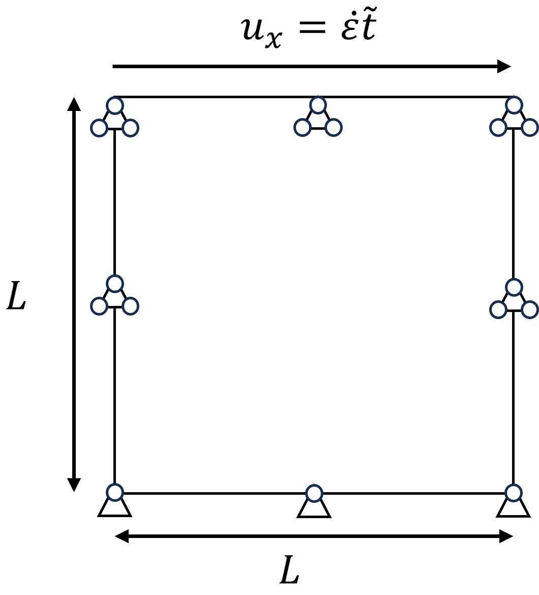
Figure 1: Numerical setup of shear in two dimensions. $\dot{\varepsilon}$ is the loading rate. $L$ is the size of the simulation square cell.

Before discussing the results, it is essential to note that the interfacial energy density $\gamma$ is related to the coefficients $\beta_{M}$ and $\beta_{g}$. Following Zhong and Zhu [45], we utilize the interfacial energy density of martensite twinnng, $187\,mJ\cdot m^{-2}$, to estimate the grid size, $l_{0}=\frac{3\gamma}{4\kappa_{M}\sqrt{2\tilde{\beta}_{M}}}=1.6\,nm$. Hence, when the simulation is performed in a domain with $N_{x}\times N_{y}=50\times 50$ mesh grids, the square simulation cell has a length $L\sim 80\,nm$.

Figure 2 presents simulation results for shear deformation on this NiTi alloy. Figure 2(a) gives the initial state of NiTi alloy. $\eta_{g}=\eta_{M}=0$ refers to the austenite and $\varepsilon^{p}=0$ comes from nondeformed alloy. Figure 2(b) shows that upon applying shear deformation to the alloy, $\eta_{M}$ (in the second row) changes from 0 to 1, i.e., the parent phase is completely transformed into martensite when the plastic strain, $\varepsilon^{p}$ (in the third row), is about 0.2. When the martensitic phase is further applied with severe shear deformation, in Figure 2(c), $\eta_{g}$ (in the first row) increases from 0 to 0.5, i.e., the amorphous phase is formed when $\varepsilon^{p}\geq 0.4$. From (b) to (c), $\eta_{M}$ changes from 1 to 0.4, which means the martensite becomes amorphous. Figure 2(d) shows that $\eta_{g}$ changes to 1 and $\eta_{M}$ decreases to 0, i.e., the entire alloy transforms into the amorphous phase when $\varepsilon^{p}\geq 0.5$.

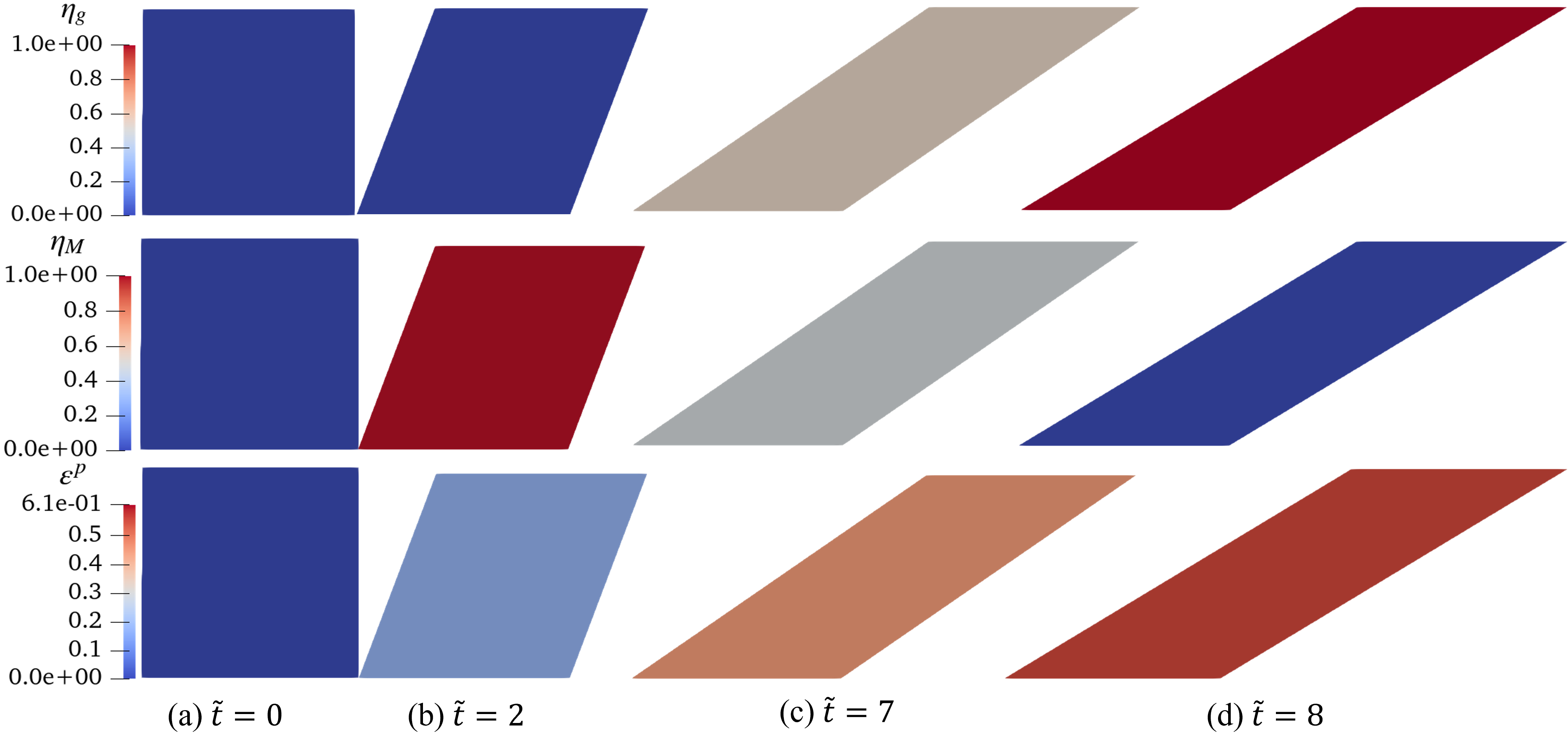
Figure 2: Results of shear in two dimensions. Three rows from top to bottom represent the evolution of order parameters $\eta_{g}$ and $\eta_{M}$, and the plastic strain $\varepsilon^{p}$. $\eta_{g}$ shows the amorphous phase while $\eta_{M}$ represents the martensite.

The evolution curves of phases are presented in Figure 3. The blue curve in Figure 3 shows $\eta_{M}$ changes from 0 to 1 when $\varepsilon^{p}$ increases to 0.18. This refers to the martensitic transformation. When $\varepsilon^{p}$ is over 0.38, $\eta_{M}$ decreases to 0, which results from amorphization. The red curve is the evolution of $\eta_{g}$, and it shows that $\eta_{g}$ remains 0 until $\varepsilon^{p}=0.38$, which is the critical plastic strain for amorphization. When the plastic strain further increases, $\eta_{g}$ increases gradually to 1. It means that the alloy completely changes to amorphous. Following the evolution curves, the austenitic phase of the NiTi alloy transforms into a martensitic phase and then into an amorphous phase under severe deformation. From this simulation, the critical plastic strain for amorphization is about 0.38 in nanocrystalline NiTi alloy. These results align well with experimental findings of strain-induced amorphization for the NiTi alloy reported by Jiang et al. [2] and Hua et al. [4], demonstrating that the proposed model is able to predict the amorphization process.

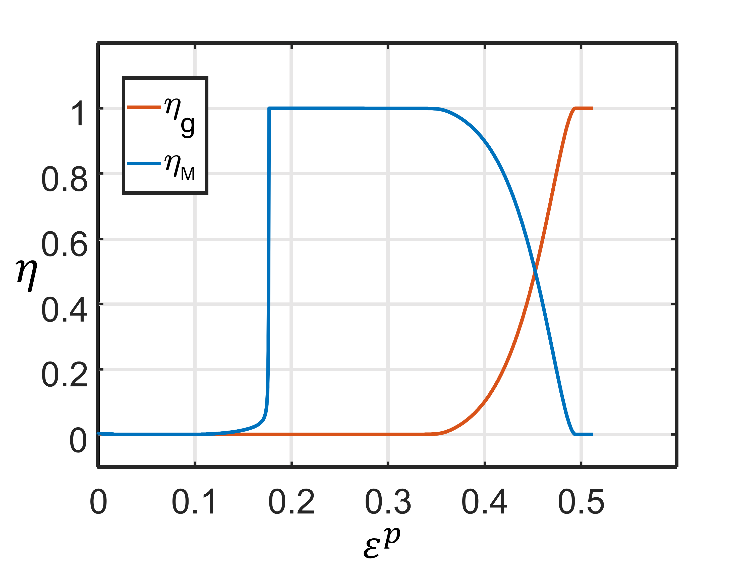
Figure 3: Results of shear in two dimensions. The horizontal ordinate denotes the plastic strain $\varepsilon^{p}$, and the vertical ordinate denotes order parameters, including $\eta_{M}$ and $\eta_{g}$. The red curve shows the evolution of $\eta_{M}$, which corresponds to the martensite, while the blue one shows the evolution of $\eta_{g}$, related to amorphous.

To illustrate the contribution from the amorphous phase during severe plastic deformation, we examine the total free energy variation under the two cases of allowing and prohibiting amorphization, and results are shown in Figure 4. In this figure, the blue curve shows the change in the total energy when amorphization is allowed in simulations. In contrast, the red curve represents the total energy when amorphization is prohibited. Both of them demonstrate that the free energy is reduced by martensitic transformation when the plastic strain $\varepsilon^{p}=0.18$. After completing the martensitic transformation, the total energy increases acceleratingly. This may result from strain-hardening of crystalline phases, making the plastic strain more difficult. As the strain exceeds the critical value of amorphization, the blue curve shows that the amorphous phase dissipates much of the total energy when it is formed. However, in the red curve, the total energy continues to increase until failure when the amorphous phase does not exist. These results demonstrate that the martensitic transformations and amorphization are essential pathways for energy dissipation for highly-deformed materials.

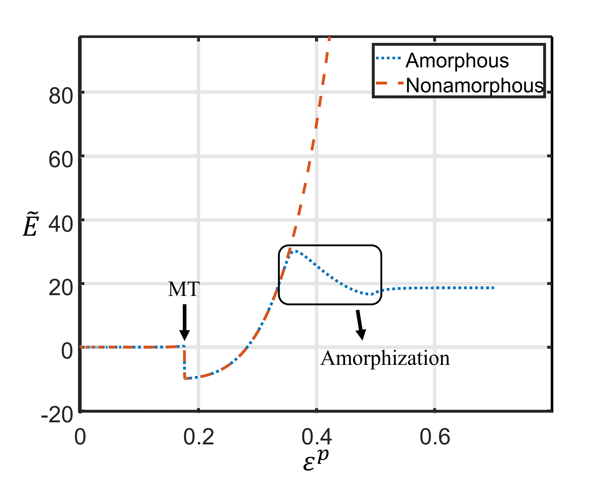
Figure 4: Evolution of the total energy in shear in two dimensions. $\tilde{E}$ denotes the dimensionless total free energy. ’MT’ means the martensitic transformation. The blue curve gives the energy curve in the simulation, which considers the amorphization. The red curve represents the evolution of the energy without nucleation of amorphous phases. The rectangle shows the change in the total energy when the amorphous phase is formed.

We further investigate the effect of grain size on amorphization using our model. We perform identical simulations on different-sized square cells to explore the size effect. In Figure 5, the blue, red, and green curves represent the evolution of $\eta_{g}$ under shear in two dimensions for domains of $L=80$, $100$, and $160\,nm$, respectively. For the critical plastic strains for amorphization, Figure 5 shows they are 0.38, 0.42, and 0.58 for cells with $L=80,100$, and $160\,nm$, respectively. When we fix the plastic strain, such as $\varepsilon^{p}=0.5$, we find that the value of the field variable, $\eta_{g}$, increases from 0 to 1 as the cell size increases. These suggest that the formation of an amorphous phase becomes increasingly difficult as the grain size increases, which is aligned with experimental findings reported by Hua et al. [3] and Fan et al. [12]. These simulation results demonstrate that the proposed model can effectively capture the nature of amorphization processes.

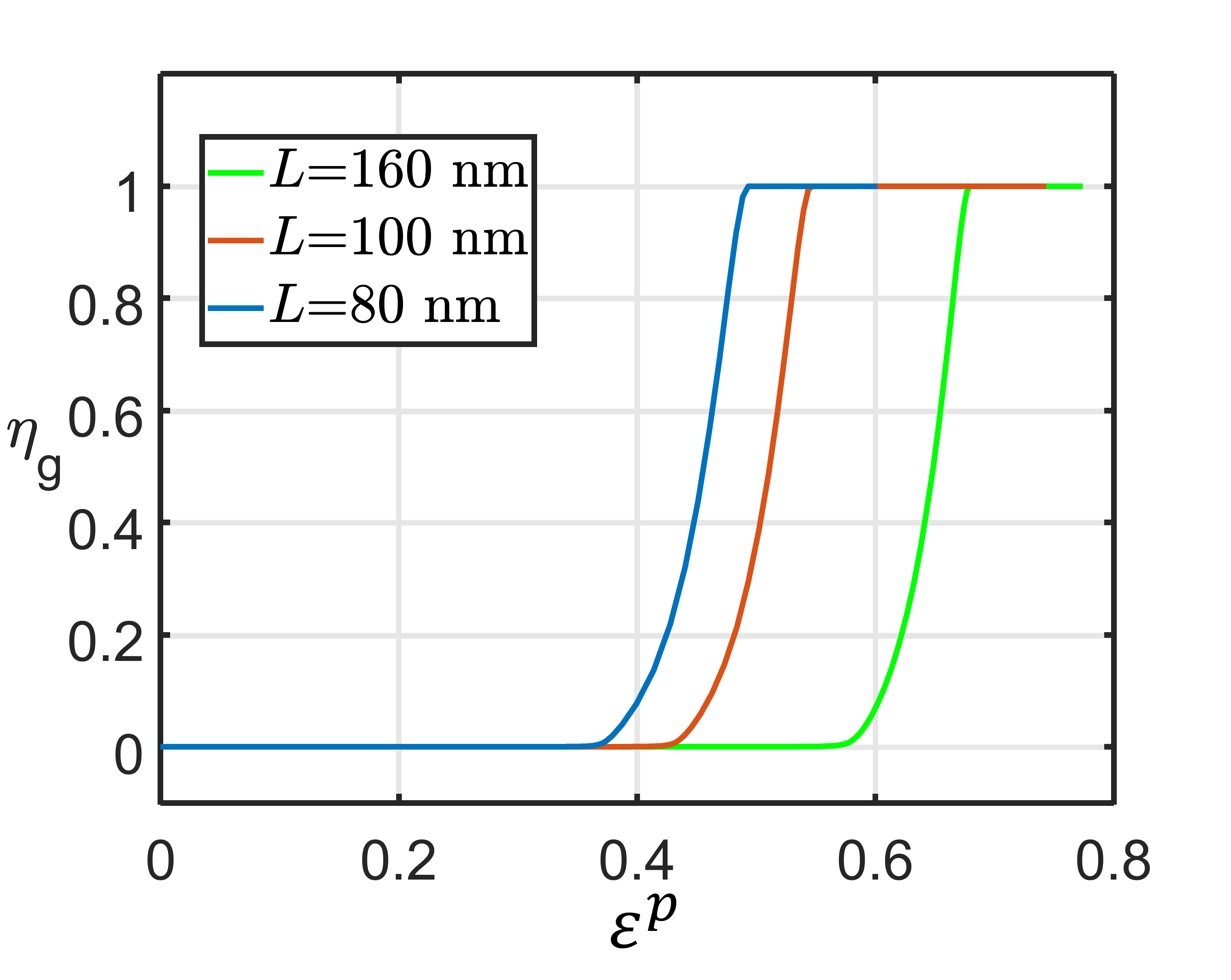
Figure 5: The amorphization curves for different domains. Three curves are green, red, and blue, representing cells with lengths of $160\,nm,100\,nm,$ and $80\,nm$, respectively.

4.2 Amorphization in shear bands

Previous studies by Hua et al. [3] and Tat’yanin et al. [30] have shown that the amorphous phase occurs in martensitic shear bands. We examine this phenomenon through numerical simulations in a 2D square cell with $L=80\,nm$. In our simulations, a shear band is introduced after the complete martensitic transformation. Parameters in this simulation are the same as those in the previous sections.

Figure 6 shows the simulation result. Figure 6(a) shows the initial state of materials. In Figure 6(b) $\eta_{M}$ (in the second row) changes to 1, which means that the martensitic transformation is completed. At this moment, a shear band is introduced in the middle of cells. Upon further shear loading, Figure 6(c) shows that $\eta_{g}$ (in the first row) increases to 0.4 in the shear band, indicating that the amorphous phase is nucleated. In Figure 6(d), $\eta_{g}$ changes to about 0.72 and $\eta_{M}$ decreases to 0.3 in the shear band, i.e., the martensite in the shear band almost completely becomes the amorphous phase. The plastic strain $\varepsilon^{p}$ (in the third row) in the shear band also increases to 0.85, which suggests that the crystalline structure is highly distorted within the shear band. From Figure 6(c) to (d), $\eta_{g}$ and $\varepsilon^{p}$ spread over the shear band. These results demonstrate that amorphous phases are formed in shear bands first and then spread out.

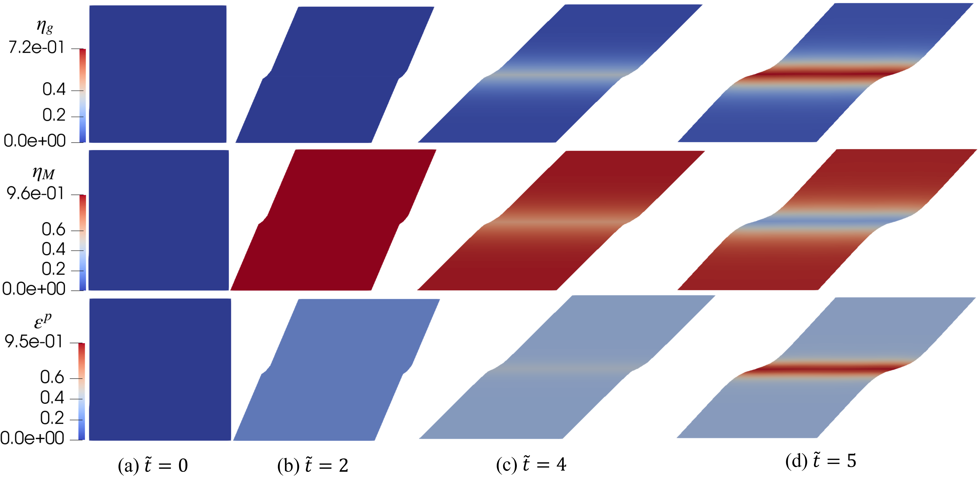
Figure 6: Amorphization in shear band. The first two rows give the evolution of the phase field variables $\eta_{M}$ and $\eta_{g}$, respectively. The last row shows the plastic behavior in the materials.

In Figure 7, we compare the amorphization behaviors of shear bands and non-localized zones. Figure 7(a) gives the material with a shear band in the middle as ’location b’, and a nonlocalized zone as ’location c’. The evolution curve in the shear band, ’location b’, is given in Figure 7(b) and in this figure, $\eta_{M}$ changes from 0 to 1, which refers to martensitic transformations. Then, $\eta_{g}$ increases gradually after $\varepsilon^{p}=0.3$, indicating that amorphization occurs within the shear band and the critical plastic strain for amorphization in the shear band is about 0.23. Figure 7(c) shows the evolution curve in the nonlocalized zone, ’location c’. It illustrates that the martensite outside the shear band does not form amorphous even when $\varepsilon^{p}=0.3$. These results indicate that shear bands significantly decrease the critical plastic strain for amorphization. This may result from the high distortion energy stored in shear bands that can overcome the formation barrier of amorphous phases.

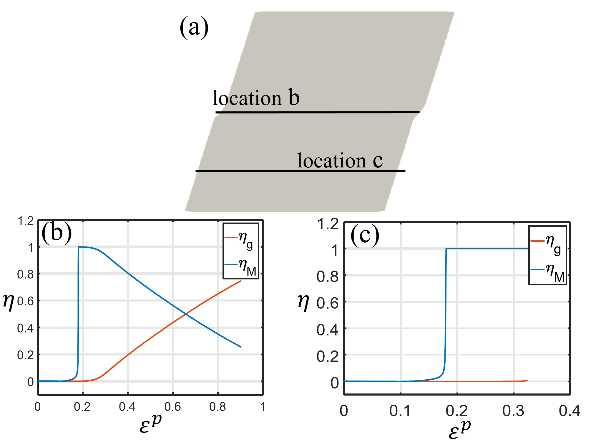
Figure 7: Comparison evolutions between the shear band and non-localized shear regions. (a) shows ’location b’ within the shear band and ’location c’ in a non-localized region. Figure (b) illustrates the evolution of phases in ’location b’. Figure (c) gives the evolutionary behavior in ’location c’ outside the shear band.

In this simulation, shear bands are simplified as localized shear-deformed areas, giving insights into the relation between amorphization and localization of deformation. These simulation results show that the critical plastic strain for amorphization decreases significantly in highly distorted regions, such as shear bands. These results suggest that localized deformation may help overcome the barrier of amorphization and reduce the threshold of plastic strain. It explains that amorphization is more likely to nucleate in shear bands and grain boundaries, as reported in previous literature [6, 3].

4.3 Compression in three dimensions

To implement our models in 3D for strain-induced amorphization, we utilize an open-source finite element framework, Multiphysics Object-Oriented Simulation Environment (MOOSE) [46]. The forward Euler method is applied in time coordinates [47].

Both simulations presented above and previous works demonstrate that the amorphous solid nucleates in the martensitic phase rather than the austenitic phase. They also imply that martensitic transformations are very fast compared to amorphization in general, meaning that it is challenging to catch details of martensitic transformations on the time scale of amorphization. The finding aligns well with experimental results in the previous studies on martensitic transformations. It suggests that we may ignore martensitic transformations and focus on the amorphization process in martensite, which also helps reduce the computational cost of our model. Following this idea, the free energy functional (29) can be reduced as,

$$E =\int_{V}\left\{e_{el}+e_{local}+e_{grad}\right\}dV,$$ (35)

$$=\int_{V}\left[\frac{1}{2}\bm{\sigma}:\bm{\varepsilon}^{el}+\kappa_{Mg}\left(\frac{A_{g}}{2}\eta_{g}^{2}-\frac{B_{g}}{3}\eta_{g}^{3}+\frac{C_{g}}{4}\eta_{g}^{4}\right)+\frac{1}{2}\beta_{g}|\nabla\eta_{g}|^{2}\right]dV,$$

where $\kappa_{Mg}$ is the energy gap between the martensitic and amorphous phase and $\beta_{g}$ is related to the interfacial energy in transition regions.

From this total free energy, we can obtain the evolution equation of phase field variable $\eta_{g}$, related to the amorphous,

$$\frac{\partial\eta_{g}}{\partial\tilde{t}} =-\left(A_{g}\eta_{g}-B_{g}\eta_{g}^{2}+C_{g}\eta_{g}^{3}\right)+\tilde{\beta}_{g}\tilde{\nabla}^{2}\eta_{g}-\frac{1}{\kappa_{Mg}}\frac{\partial e_{el}}{\partial\eta_{g}},$$ (36)

and this equation is normalized by following the same method for (34).

The simulation is performed in a cubic cell of size $L=170\,nm$, with a random initial value between 0 and 0.1 assigned to the phase variable $\eta_{g}$. The compression along the $Z$ axis is applied to the nanocrystalline NiTi shape alloy, whose mechanical properties are $\dot{\gamma}^{0}=1\times 10^{-4}$, $m=6$, $h=1\,GPa$ and the yield stress $\tau_{c,0}=2.7\,GPa$. For amorphous phases, $\frac{1}{A}=5\times 10^{-5}$, $\sigma_{0}=1.2\,GPa$ are used. All thermodynamic parameters are set as follows: $\kappa_{Mg}=4.403\times 10^{8}\,J\cdot m^{-3}$, $A_{g}=3$, $B_{g}=12$, $C_{g}=14$. The gradient coefficient $\tilde{\beta}_{g}$ is set to 1, and the interfacial energy density of transition regions is assumed to be $706\,mJ\cdot m^{-2}$ [9]. Based on these parameters, we can estimate the grid size as $l_{0}\approx 8.5\,nm$, and we use a cubic cell of $N_{x}\times N_{y}\times N_{z}=20\times 20\times 20$, giving the length of the cubic domain as $\sim 170\,nm$.

Figure 8 shows the results of this compression simulation in 3D. The first row in Figure 8 provides a 3D overview of the distributions of amorphous and stress in the compressed alloy. The second, third, and fourth rows show some clips of the simulation cell along the Y-Z, X-Z, and X-Y planes, respectively. The phase variable for the amorphous phase, $\eta_{g}$ is given in the left column, and the magnitude of stress $\sigma_{x}=\sqrt{\sigma_{xx}^{2}+\sigma_{xy}^{2}+\sigma_{xz}^{2}}$ is given in the right column. As shown in Figure 8, the amorphous phase is mostly nucleated on the surfaces and interior regions under high stress.

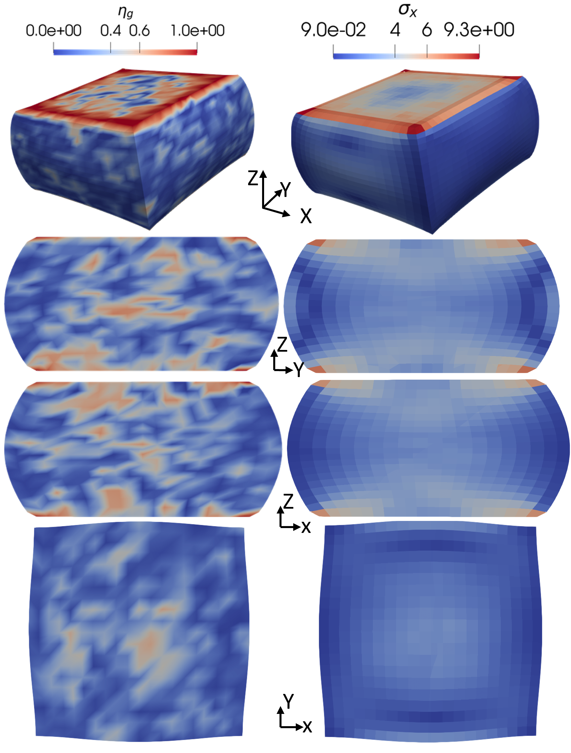
Figure 8: Results of compression in three dimensions. The first row illustrates a general picture of the distributions of the order parameter $\eta_{g}$ (left), which relates to the amorphous phase and the magnitude of stress $\sigma_{x}$ (right). The following three rows show the clips along the Y-Z, X-Z, and X-Y planes of $\eta_{g}$ (left) and $\sigma_{x}$ (right), respectively.

Figure 9 shows the isosurfaces of the phase variable $\eta_{g}=0.5$, considered as a threshold for amorphization. In Figure 9(a) and (b), amorphous phases are formed on the surfaces, when the compression strain $\varepsilon_{c}\leq 0.302$. Under further compression deformation, as shown in Figure 9(c) and (d), the isosurfaces roughly align with the diagonal regions and surfaces of the compressed cell, which generally refer to highly distorted regions. These results suggest that amorphous phases are formed in highly-distorted areas, such as surfaces and diagonal regions in the compressed alloy. This is consistent with experimental observations made by Guo et al. [31] and Zhao et al. [32].

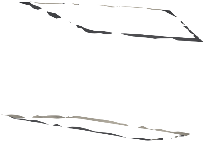
(a) $\varepsilon_{c}=0.228$

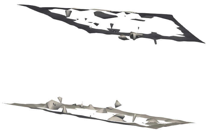
(b) $\varepsilon_{c}=0.302$

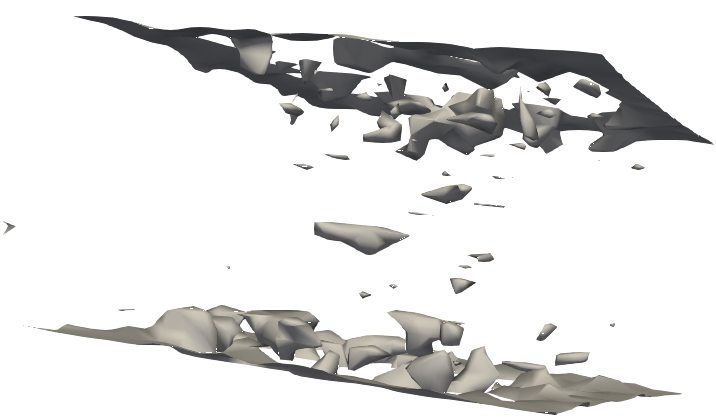
(c) $\varepsilon_{c}=0.332$

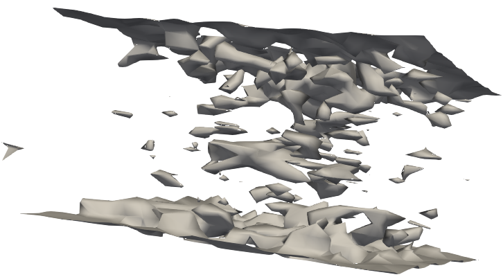
(d) $\varepsilon_{c}=0.365$

Figure 9: Isosurfaces of $\eta_{g}=0.5$. The compressed strain applied in the alloy is represented by $\varepsilon_{c}$. Figure (a) to (d) show the evolution of region where $\eta_{g}=0.5$ upon loading.

Figure 10 gives the curve of the volume fraction of amorphous phases $V_{g}$ vs. the applied strain $\varepsilon_{c}$. In Figure 10, the amorphous phase forms until the compressed strain $\varepsilon_{c}>0.25$. When $\varepsilon_{c}=0.35$, the volume fraction of the amorphous phase $V_{g}$ attains 0.15. These quantitative predictions align with experimental findings in the nanocrystalline NiTi alloy [3], validating our model in predicting strain-induced amorphization.

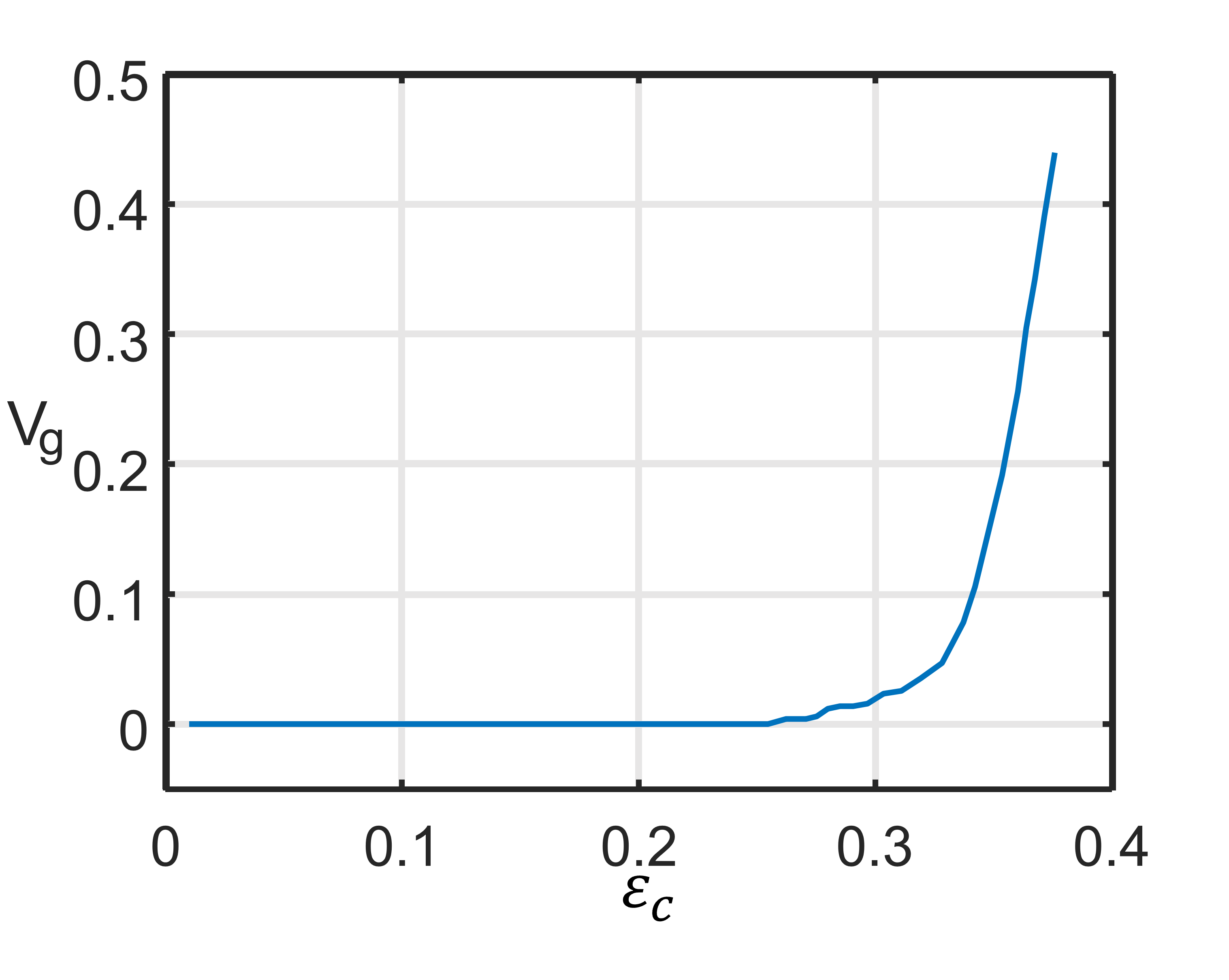
Figure 10: The curve of amorphization under compression. $V_{g}$ represents the volume fraction of the amorphous phase, and $\varepsilon_{c}$ is the applied strain.

5 Conclusions

We introduce a phase field model to investigate deformation-induced amorphization at large strains. The proposed phase-field model incorporates martensitic transformations and amorphization using two phase field variables. The elastic-plastic theory is coupled with our model through the strain energy, which drives the amorphization during severe deformations. Various microscopic mechanisms related to amorphization, such as shear bands, can be explored using this coupled model. We perform numerical simulations to validate the proposed model and quantitatively study the strain-induced amorphization. Simulation results show that amorphization occurs within the martensitic phases rather than the austenitic phase. The effect of the grain size on amorphization is investigated and simulation results demonstrate that the critical plastic strain of amorphization increases as the grain size increases. Shear bands are considered in our simulations and the results show that the amorphous phase is formed within shear bands and then spread out. The simulation on compression in 3D also shows that nucleation of amorphous phases occurs in diagonal regions and on surfaces, which refer to highly-distorted areas in the compressed cell. These simulation results from shear bands and compression indicate that defects and high distortion in materials facilitate favorable conditions for the formation of amorphous phases. These observations align well with experimental results from previous works, validating the proposed model. This novel phase field model lays the groundwork for more quantitative theories of deformation-induced amorphization and provides a realistic tool for studying the underlying mechanisms of amorphization. Some simplifications for efficient simulations, including linear elasticity, might limit the investigation into amorphization under large deformations. Considering further work, the developments of various defects, which play a significant role in the amorphization process, such as dislocations and grain boundaries, can be investigated using our model.

Appendix: Symbols

Table 1: List of symbols

Symbol	Meaning
$\eta_{M}$/$\eta_{g}$	Order parameter for the martensite/amorphous phase
$\Omega_{0}$ /$\Omega$	Reference/deformed configuration
$\bm{x}$	Material point in $\Omega_{0}$
$\bm{X}$	Image point in $\Omega$
$\bm{F}$	Total deformation gradient
$\bm{F}_{e}$/$\bm{F}_{p}$	Elastic/inelastic part of deformation gradient
$\bm{L}_{p}$	Plastic velocity gradient
$N_{s}$	Number of slip systems in crystal
$\alpha,\beta$	Indices of slip systems
$\dot{\gamma}^{\alpha}$	Shear rate on slip system $\alpha$
$\bm{m}^{\alpha}$	Slip direction on slip system $\alpha$
$\bm{n}^{\alpha}$	Slip normal of slip system $\alpha$
$\bm{L}_{g}^{p}$	Plastic velocity in amorphous regions
$\tau^{\alpha}$	Resolved stress on the slip system $\alpha$
$\dot{\gamma}_{0}$ and $m$	Material constants for crystal phases
$\tau_{c}^{\alpha}$	Slip resistance on the slip system $\alpha$
$h_{\alpha\beta}$	Hardening matrix
$\tau_{D,d}$	Deviatoric Kirchhoff stress tensor
$\bm{N}$	Visco-plastic flow vector
$\dot{\gamma}_{g}$	Visco-plastic multiplier
$\bm{R}_{e}$	Elastic rotation tensor
$A$	Eyring-relation function for amorphous phase
$\tau_{D}^{eq}$	Kirchhoff equivalent stress
$\tau^{*}$	Reference stress for amorphous phase
$E$	Total energy functional
$E_{local}(e_{local})$	Local phase separation energy (density)
$E_{grad}(e_{grad})$	Gradient energy (density)
$E_{el}(e_{el})$	Elastic strain energy (density)
$A_{M},B_{M},C_{M},$ $A_{g},B_{g},C_{g},D$	Parameters determine phase separation energy
$\kappa_{M}$/$\kappa_{g}$	Energy gap between the austenite and martensite/amorphous
$\kappa_{Mg}$	Energy barrier for the co-existence of martensite and amorphous
$f_{\eta_{M}}^{local}$	Driving force for $\eta_{M}$ related with $e_{local}$
$f_{\eta_{g}}^{local}$	Driving force for $\eta_{g}$ related with $e_{local}$
$\beta_{M},\beta_{g}$	Coefficients related to the interfacial energy
$f_{\eta_{M}}^{grad}$	Driving force for $\eta_{M}$ related with $e_{grad}$
$f_{\eta_{g}}^{grad}$	Driving force for $\eta_{g}$ related with $e_{grad}$
$\bm{E}_{e}$	Elastic strain tensor
$\mathbb{C}$	Elastic coefficients in mixed regions
$\mathbb{C}_{A}$/ $\mathbb{C}_{M}$/ $\mathbb{C}_{g}$	Elastic coefficients in the austenite/martensite/ amorphous
$\bm{P}$	First Piola-Kirchhoff stress tensor
$\bm{C}_{e}$	Elastic deformation tensor
$f_{\eta_{M}}^{el}$	Driving force for $\eta_{M}$ related with $e_{el}$
$f_{\eta_{g}}^{el}$	Driving force for $\eta_{g}$ related with $e_{el}$
$M_{M},M_{g}$	Mobilities for the martensite and amorphous
$\bm{\varepsilon}^{M}$	Eigenstrain of martensitic transformation
$\bm{\varepsilon}_{crsytal}^{p}$	Plastic strain in crystalline phases
$\bm{\varepsilon}^{p}_{g}$	Plastic strain in amorphous
$\bm{S}$	Deviatoric stress tensor

References

- Waitz et al. [2004] T. Waitz, V. Kazykhanov, and H.P. Karnthaler. Martensitic phase transformations in nanocrystalline NiTi studied by TEM. Acta Materialia, 52(1):137–147, January 2004. ISSN 13596454. doi: 10.1016/j.actamat.2003.08.036. URL https://linkinghub.elsevier.com/retrieve/pii/S1359645403005184.
- Jiang et al. [2013] Shuyong Jiang, Li Hu, Yanqiu Zhang, and Yulong Liang. Nanocrystallization and amorphization of NiTi shape memory alloy under severe plastic deformation based on local canning compression. Journal of Non-Crystalline Solids, 367:23–29, May 2013. ISSN 00223093. doi: 10.1016/j.jnoncrysol.2013.01.051. URL https://linkinghub.elsevier.com/retrieve/pii/S0022309313000732.
- Hua et al. [2022] Peng Hua, Bing Wang, Chao Yu, Yilong Han, and Qingping Sun. Shear-induced amorphization in nanocrystalline NiTi micropillars under large plastic deformation. Acta Materialia, 241:118358, December 2022. ISSN 13596454. doi: 10.1016/j.actamat.2022.118358. URL https://linkinghub.elsevier.com/retrieve/pii/S1359645422007376.
- Hua et al. [2021] Peng Hua, Minglu Xia, Yusuke Onuki, and Qingping Sun. Nanocomposite NiTi shape memory alloy with high strength and fatigue resistance. Nature Nanotechnology, 16(4):409–413, April 2021. ISSN 1748-3387, 1748-3395. doi: 10.1038/s41565-020-00837-5. URL https://www.nature.com/articles/s41565-020-00837-5.
- Idrissi et al. [2022] Hosni Idrissi, Philippe Carrez, and Patrick Cordier. On amorphization as a deformation mechanism under high stresses. Current Opinion in Solid State and Materials Science, 26(1):100976, February 2022. ISSN 13590286. doi: 10.1016/j.cossms.2021.100976. URL https://linkinghub.elsevier.com/retrieve/pii/S1359028621000796.
- Li et al. [2022] B.Y. Li, A.C. Li, S. Zhao, and M.A. Meyers. Amorphization by mechanical deformation. Materials Science and Engineering: R: Reports, 149:100673, June 2022. ISSN 0927796X. doi: 10.1016/j.mser.2022.100673. URL https://linkinghub.elsevier.com/retrieve/pii/S0927796X22000122.
- Miyagi et al. [2011] Lowell Miyagi, Waruntorn Kanitpanyacharoen, Stephen Stackhouse, Burkhard Militzer, and Hans-Rudolf Wenk. The enigma of post-perovskite anisotropy: deformation versus transformation textures. Physics and Chemistry of Minerals, 38(9):665–678, October 2011. ISSN 1432-2021. doi: 10.1007/s00269-011-0439-y. URL https://doi.org/10.1007/s00269-011-0439-y.
- Koike et al. [1990] Jun-ichi Koike, D. M. Parkin, and M. Nastasi. The role of shear instability in amorphization of cold-rolled NiTi. Philosophical Magazine Letters, 62(4):257–264, October 1990. ISSN 0950-0839, 1362-3036. doi: 10.1080/09500839008215132. URL http://www.tandfonline.com/doi/abs/10.1080/09500839008215132.
- Yamada and Koch [1993] Kenjiro Yamada and Carl C. Koch. The influence of mill energy and temperature on the structure of the TiNi intermetallic after mechanical attrition. Journal of Materials Research, 8(6):1317–1326, June 1993. ISSN 0884-2914, 2044-5326. doi: 10.1557/JMR.1993.1317. URL http://link.springer.com/10.1557/JMR.1993.1317.
- Jiang et al. [2017] Shuyong Jiang, Zhinan Mao, Yanqiu Zhang, and Li Hu. Mechanisms of nanocrystallization and amorphization of NiTiNb shape memory alloy subjected to severe plastic deformation. Procedia Engineering, 207:1493–1498, 2017. ISSN 18777058. doi: 10.1016/j.proeng.2017.10.1086. URL https://linkinghub.elsevier.com/retrieve/pii/S187770581735885X.
- Zhang et al. [2018] Long Zhang, Haifeng Zhang, Xiaobing Ren, Jürgen Eckert, Yandong Wang, Zhengwang Zhu, Thomas Gemming, and Simon Pauly. Amorphous martensite in -Ti alloys. Nature Communications, 9(1):506, February 2018. ISSN 2041-1723. doi: 10.1038/s41467-018-02961-2. URL https://www.nature.com/articles/s41467-018-02961-2.
- Fan et al. [2018] Jinjun Fan, Jia Li, Zaiwang Huang, P.H. Wen, and C.G. Bailey. Grain size effects on indentation-induced plastic deformation and amorphization process of polycrystalline silicon. Computational Materials Science, 144:113–119, March 2018. ISSN 09270256. doi: 10.1016/j.commatsci.2017.12.017. URL https://linkinghub.elsevier.com/retrieve/pii/S0927025617307024.
- Xu and Kang [2021] Bo Xu and Guozheng Kang. Phase field simulation on the super-elasticity, elastocaloric and shape memory effect of geometrically graded nano-polycrystalline NiTi shape memory alloys. International Journal of Mechanical Sciences, 201:106462, July 2021. ISSN 00207403. doi: 10.1016/j.ijmecsci.2021.106462. URL https://linkinghub.elsevier.com/retrieve/pii/S0020740321001971.
- Basak and Levitas [2023] Anup Basak and Valery I. Levitas. A multiphase phase-field study of three-dimensional martensitic twinned microstructures at large strains. Continuum Mechanics and Thermodynamics, 35(4):1595–1624, July 2023. ISSN 0935-1175, 1432-0959. doi: 10.1007/s00161-022-01177-6. URL https://link.springer.com/10.1007/s00161-022-01177-6.
- Mirzakhani and Javanbakht [2018] Sam Mirzakhani and Mahdi Javanbakht. Phase field-elasticity analysis of austenite–martensite phase transformation at the nanoscale: Finite element modeling. Computational Materials Science, 154:41–52, November 2018. ISSN 09270256. doi: 10.1016/j.commatsci.2018.07.034. URL https://linkinghub.elsevier.com/retrieve/pii/S0927025618304622.
- Artemev et al. [2001] A. Artemev, Y. Jin, and A.G. Khachaturyan. Three-dimensional phase field model of proper martensitic transformation. Acta Materialia, 49(7):1165–1177, April 2001. ISSN 13596454. doi: 10.1016/S1359-6454(01)00021-0. URL https://linkinghub.elsevier.com/retrieve/pii/S1359645401000210.
- Borukhovich et al. [2015] Efim Borukhovich, Philipp S. Engels, Jörn Mosler, Oleg Shchyglo, and Ingo Steinbach. Large deformation framework for phase-field simulations at the mesoscale. Computational Materials Science, 108:367–373, October 2015. ISSN 09270256. doi: 10.1016/j.commatsci.2015.06.021. URL https://linkinghub.elsevier.com/retrieve/pii/S0927025615003808.
- Basak and Levitas [2019] Anup Basak and Valery I. Levitas. Finite element procedure and simulations for a multiphase phase field approach to martensitic phase transformations at large strains and with interfacial stresses. Computer Methods in Applied Mechanics and Engineering, 343:368–406, January 2019. ISSN 00457825. doi: 10.1016/j.cma.2018.08.006. URL https://linkinghub.elsevier.com/retrieve/pii/S004578251830392X.
- Finel et al. [2010] Alphonse Finel, Y. Le Bouar, A. Gaubert, and U. Salman. Phase field methods: Microstructures, mechanical properties and complexity. Comptes Rendus Physique, 11(3-4):245–256, April 2010. ISSN 16310705. doi: 10.1016/j.crhy.2010.07.014. URL https://linkinghub.elsevier.com/retrieve/pii/S1631070510000794.
- Steinbach and Shchyglo [2011] Ingo Steinbach and Oleg Shchyglo. Phase-field modelling of microstructure evolution in solids: Perspectives and challenges. Current Opinion in Solid State and Materials Science, 15(3):87–92, June 2011. ISSN 13590286. doi: 10.1016/j.cossms.2011.01.001. URL https://linkinghub.elsevier.com/retrieve/pii/S1359028611000027.
- Biner [2017] S. Bulent Biner. Programming Phase-Field Modeling. Springer International Publishing, Cham, 2017. ISBN 978-3-319-41194-1 978-3-319-41196-5. doi: 10.1007/978-3-319-41196-5. URL http://link.springer.com/10.1007/978-3-319-41196-5.
- Schneider et al. [2017] Daniel Schneider, Felix Schwab, Ephraim Schoof, Andreas Reiter, Christoph Herrmann, Michael Selzer, Thomas Böhlke, and Britta Nestler. On the stress calculation within phase-field approaches: a model for finite deformations. Computational Mechanics, 60(2):203–217, August 2017. ISSN 0178-7675, 1432-0924. doi: 10.1007/s00466-017-1401-8. URL http://link.springer.com/10.1007/s00466-017-1401-8.
- Steinbach et al. [1996] I. Steinbach, F. Pezzolla, B. Nestler, M. Seeßelberg, R. Prieler, G.J. Schmitz, and J.L.L. Rezende. A phase field concept for multiphase systems. Physica D: Nonlinear Phenomena, 94(3):135–147, July 1996. ISSN 01672789. doi: 10.1016/0167-2789(95)00298-7. URL https://linkinghub.elsevier.com/retrieve/pii/0167278995002987.
- Levitas [1998] Valery I. Levitas. Thermomechanical theory of martensitic phase transformations in inelastic materials. International Journal of Solids and Structures, 35(9-10):889–940, March 1998. ISSN 00207683. doi: 10.1016/S0020-7683(97)00089-9. URL https://linkinghub.elsevier.com/retrieve/pii/S0020768397000899.
- Clayton and Knap [2011] J.D. Clayton and J. Knap. A phase field model of deformation twinning: Nonlinear theory and numerical simulations. Physica D: Nonlinear Phenomena, 240(9-10):841–858, April 2011. ISSN 01672789. doi: 10.1016/j.physd.2010.12.012. URL https://linkinghub.elsevier.com/retrieve/pii/S0167278910003623.
- Tsuchiya et al. [2006] K. Tsuchiya, M. Inuzuka, D. Tomus, A. Hosokawa, H. Nakayama, K. Morii, Y. Todaka, and M. Umemoto. Martensitic transformation in nanostructured TiNi shape memory alloy formed via severe plastic deformation. Materials Science and Engineering: A, 438-440:643–648, November 2006. ISSN 09215093. doi: 10.1016/j.msea.2006.01.110. URL https://linkinghub.elsevier.com/retrieve/pii/S0921509306006320.
- Levin et al. [2013] Vladimir A. Levin, Valery I. Levitas, Konstantin M. Zingerman, and Eugene I. Freiman. Phase-field simulation of stress-induced martensitic phase transformations at large strains. International Journal of Solids and Structures, 50(19):2914–2928, September 2013. ISSN 00207683. doi: 10.1016/j.ijsolstr.2013.05.003. URL https://linkinghub.elsevier.com/retrieve/pii/S0020768313001959.
- Levitas [2013] Valery I. Levitas. Phase-field theory for martensitic phase transformations at large strains. International Journal of Plasticity, 49:85–118, October 2013. ISSN 07496419. doi: 10.1016/j.ijplas.2013.03.002. URL https://linkinghub.elsevier.com/retrieve/pii/S0749641913000727.
- Yeddu et al. [2012] Hemantha Kumar Yeddu, Amer Malik, John Ågren, Gustav Amberg, and Annika Borgenstam. Three-dimensional phase-field modeling of martensitic microstructure evolution in steels. Acta Materialia, 60(4):1538–1547, February 2012. ISSN 13596454. doi: 10.1016/j.actamat.2011.11.039. URL https://linkinghub.elsevier.com/retrieve/pii/S1359645411008299.
- Tat’yanin et al. [1997] E. V. Tat’yanin, N. F. Borovikov, V. G. Kurdyumov, and V. L. Indenbom. Amorphous shear bands in deformed TiNi alloy. Physics of the Solid State, 39(7):1097–1099, July 1997. ISSN 1063-7834, 1090-6460. doi: 10.1134/1.1130038. URL http://link.springer.com/10.1134/1.1130038.
- Guo et al. [2018] Wei Guo, Yifei Meng, Xie Zhang, Vikram Bedekar, Hongbin Bei, Scott Hyde, Qianying Guo, Gregory B. Thompson, Rajiv Shivpuri, Jian-min Zuo, and Jonathan D. Poplawsky. Extremely hard amorphous-crystalline hybrid steel surface produced by deformation induced cementite amorphization. Acta Materialia, 152:107–118, June 2018. ISSN 13596454. doi: 10.1016/j.actamat.2018.04.013. URL https://linkinghub.elsevier.com/retrieve/pii/S1359645418302866.
- Zhao et al. [2016] S. Zhao, E.N. Hahn, B. Kad, B.A. Remington, C.E. Wehrenberg, E.M. Bringa, and M.A. Meyers. Amorphization and nanocrystallization of silicon under shock compression. Acta Materialia, 103:519–533, January 2016. ISSN 13596454. doi: 10.1016/j.actamat.2015.09.022. URL https://linkinghub.elsevier.com/retrieve/pii/S1359645415006916.
- Malik et al. [2013] Amer Malik, Gustav Amberg, Annika Borgenstam, and John Ågren. Effect of external loading on the martensitic transformation – A phase field study. Acta Materialia, 61(20):7868–7880, December 2013. ISSN 13596454. doi: 10.1016/j.actamat.2013.09.025. URL https://linkinghub.elsevier.com/retrieve/pii/S1359645413007106.
- Xu et al. [2020] Bo Xu, Guozheng Kang, Qianhua Kan, Chao Yu, and Xi Xie. Phase field simulation on the cyclic degeneration of one-way shape memory effect of NiTi shape memory alloy single crystal. International Journal of Mechanical Sciences, 168:105303, February 2020. ISSN 00207403. doi: 10.1016/j.ijmecsci.2019.105303. URL https://linkinghub.elsevier.com/retrieve/pii/S0020740319330164.
- Vattré and Denoual [2016] A. Vattré and C. Denoual. Polymorphism of iron at high pressure: A 3D phase-field model for displacive transitions with finite elastoplastic deformations. Journal of the Mechanics and Physics of Solids, 92:1–27, July 2016. ISSN 00225096. doi: 10.1016/j.jmps.2016.01.016. URL https://linkinghub.elsevier.com/retrieve/pii/S0022509616000181.
- Ma and Sun [2021] Ran Ma and WaiChing Sun. Phase field modeling of coupled crystal plasticity and deformation twinning in polycrystals with monolithic and splitting solvers. International Journal for Numerical Methods in Engineering, 122(4):1167–1189, February 2021. ISSN 0029-5981, 1097-0207. doi: 10.1002/nme.6577. URL https://onlinelibrary.wiley.com/doi/10.1002/nme.6577.
- Liu et al. [2018] C. Liu, P. Shanthraj, M. Diehl, F. Roters, S. Dong, J. Dong, W. Ding, and D. Raabe. An integrated crystal plasticity–phase field model for spatially resolved twin nucleation, propagation, and growth in hexagonal materials. International Journal of Plasticity, 106:203–227, July 2018. ISSN 07496419. doi: 10.1016/j.ijplas.2018.03.009. URL https://linkinghub.elsevier.com/retrieve/pii/S0749641917307209.
- Roters et al. [2010] F. Roters, P. Eisenlohr, L. Hantcherli, D.D. Tjahjanto, T.R. Bieler, and D. Raabe. Overview of constitutive laws, kinematics, homogenization and multiscale methods in crystal plasticity finite-element modeling: Theory, experiments, applications. Acta Materialia, 58(4):1152–1211, February 2010. ISSN 13596454. doi: 10.1016/j.actamat.2009.10.058. URL https://linkinghub.elsevier.com/retrieve/pii/S1359645409007617.
- Sarma et al. [1998] G.B. Sarma, B. Radhakrishnan, and T. Zacharia. Finite element simulations of cold deformation at the mesoscale. Computational Materials Science, 12(2):105–123, September 1998. ISSN 09270256. doi: 10.1016/S0927-0256(98)00036-6. URL https://linkinghub.elsevier.com/retrieve/pii/S0927025698000366.
- Ferreira et al. [2023] Bernardo P. Ferreira, A. Francisca Carvalho Alves, and F.M. Andrade Pires. An efficient finite strain constitutive model for amorphous thermoplastics: Fully implicit computational implementation and optimization-based parameter calibration. Computers & Structures, 281:107007, June 2023. ISSN 00457949. doi: 10.1016/j.compstruc.2023.107007. URL https://linkinghub.elsevier.com/retrieve/pii/S0045794923000378.
- Schuh et al. [2007] C Schuh, T Hufnagel, and U Ramamurty. Mechanical behavior of amorphous alloys. Acta Materialia, 55(12):4067–4109, July 2007. ISSN 13596454. doi: 10.1016/j.actamat.2007.01.052. URL https://linkinghub.elsevier.com/retrieve/pii/S135964540700122X.
- Kassner et al. [2015] Michael E. Kassner, Kamia Smith, and Veronica Eliasson. Creep in amorphous metals. Journal of Materials Research and Technology, 4(1):100–107, January 2015. ISSN 22387854. doi: 10.1016/j.jmrt.2014.11.003. URL https://linkinghub.elsevier.com/retrieve/pii/S2238785414001100.
- Gao [2006] Y F Gao. An implicit finite element method for simulating inhomogeneous deformation and shear bands of amorphous alloys based on the free-volume model. Modelling and Simulation in Materials Science and Engineering, 14(8):1329–1345, December 2006. ISSN 0965-0393, 1361-651X. doi: 10.1088/0965-0393/14/8/004. URL https://iopscience.iop.org/article/10.1088/0965-0393/14/8/004.
- Gurtin and Anand [2005] Morton E. Gurtin and Lallit Anand. The decomposition F=FeFp, material symmetry, and plastic irrotationality for solids that are isotropic-viscoplastic or amorphous. International Journal of Plasticity, 21(9):1686–1719, September 2005. ISSN 07496419. doi: 10.1016/j.ijplas.2004.11.007. URL https://linkinghub.elsevier.com/retrieve/pii/S0749641904001603.
- Zhong and Zhu [2014] Yuan Zhong and Ting Zhu. Phase-field modeling of martensitic microstructure in NiTi shape memory alloys. Acta Materialia, 75:337–347, August 2014. ISSN 13596454. doi: 10.1016/j.actamat.2014.04.013. URL https://linkinghub.elsevier.com/retrieve/pii/S1359645414002523.
- Lindsay et al. [2022] Alexander D. Lindsay, Derek R. Gaston, Cody J. Permann, Jason M. Miller, David Andrš, Andrew E. Slaughter, Fande Kong, Joshua Hansel, Robert W. Carlsen, Casey Icenhour, Logan Harbour, Guillaume L. Giudicelli, Roy H. Stogner, Peter German, Jacob Badger, Sudipta Biswas, Leora Chapuis, Christopher Green, Jason Hales, Tianchen Hu, Wen Jiang, Yeon Sang Jung, Christopher Matthews, Yinbin Miao, April Novak, John W. Peterson, Zachary M. Prince, Andrea Rovinelli, Sebastian Schunert, Daniel Schwen, Benjamin W. Spencer, Swetha Veeraraghavan, Antonio Recuero, Dewen Yushu, Yaqi Wang, Andy Wilkins, and Christopher Wong. 2.0 - MOOSE: Enabling massively parallel multiphysics simulation. SoftwareX, 20:101202, 2022. ISSN 2352-7110. doi: https://doi.org/10.1016/j.softx.2022.101202. URL https://www.sciencedirect.com/science/article/pii/S2352711022001200.
- She et al. [2013] Hui She, Yulan Liu, Biao Wang, and Decai Ma. Finite element simulation of phase field model for nanoscale martensitic transformation. Computational Mechanics, 52(4):949–958, October 2013. ISSN 0178-7675, 1432-0924. doi: 10.1007/s00466-013-0856-5. URL http://link.springer.com/10.1007/s00466-013-0856-5.