GraphBPE: Molecular Graphs Meet Byte-Pair Encoding

Abstract

With the increasing attention to molecular machine learning, various innovations have been made in designing better models or proposing more comprehensive benchmarks. However, less is studied on the data preprocessing schedule for molecular graphs, where a different view of the molecular graph could potentially boost the model’s performance. Inspired by the Byte-Pair Encoding (BPE) algorithm, a subword tokenization method popularly adopted in Natural Language Processing, we propose GraphBPE, which tokenizes a molecular graph into different substructures and acts as a preprocessing schedule independent of the model architectures. Our experiments on 3 graph-level classification and 3 graph-level regression datasets show that data preprocessing could boost the performance of models for molecular graphs, and GraphBPE is effective for small classification datasets and it performs on par with other tokenization methods across different model architectures.

1 Introduction

Tokenization (Sennrich et al., 2016; Schuster & Nakajima, 2012; Kudo, 2018; Kudo & Richardson, 2018) is an important building block that contributes to the success of modern Natural Language Processing (NLP) applications such as Large Language Models (LLMs) (Brown et al., 2020; Touvron et al., 2023a; Almazrouei et al., 2023; Touvron et al., 2023b). Before being fed into a model, each word in the input sentence is first tokenized into subwords (e.g., $\text{``lowest''}\rightarrow\text{``low'', ``est''}$), which may not necessarily convey meaningful semantics but facilitates the learning of the model. Among different tokenization methods, Byte-Pair Encoding (BPE) (Gage, 1994; Sennrich et al., 2016) is a popularly adopted mechanism. Given a text corpus containing numerous sentences and thus words, BPE counts the appearance of two consecutive tokens (e.g., a subword “es”, an English letter “t”) in each word at each iteration, and merges the token pair with the highest frequency and treats it as the new token (e.g., $\text{``es'', ``t''}\rightarrow\text{``est''}$) for next round. A vocabulary containing a variety of subwords is then learned after some iterations, and later used to tokenize sentences fed to the model.

It is easy to observe that this “count-and-merge” schedule has the potential to generalize beyond texts into arbitrary structures such as molecular graphs. Indeed, we can view words as line graphs, where each character in the word is the node, and the edges are defined by whether two characters are contiguous in the word. This observation naturally motivates us to explore the following questions: a). “Can graphs be tokenized similarly to that of texts?” b). “Will the tokenized graphs improve the model performance?”

To investigate whether molecular graphs can be tokenized similarly to texts, we develop GraphBPE, a variant of the BPE algorithm for molecular graphs, which counts the co-occurrence of contextualized (e.g., neighborhood-aware) node pairs (e.g., defined by edges) and merges the most frequent pair as the new node for next round. Compared with other methods (Jin et al., 2020; Li et al., 2023) that require external knowledge (e.g., functional groups, a trained neural network) to mine substructures, our algorithm relies solely on a given molecular graph corpus and is model agnostic. After each round of tokenization, the resulting new graph is still connected with its nodes being subsets of the nodes of the previous graph, which provides a view to construct both simple graphs and hypergraphs (Section 3.2) that can be used by Graph Neural Networks (GNNs) (Kipf & Welling, 2017; Veličković et al., 2018; Xu et al., 2019; Hamilton et al., 2018) and Hypergraph Neural Networks (HyperGNNs) (Feng et al., 2019; Bai et al., 2020; Dong et al., 2020; Gao et al., 2023).

To explore whether tokenization helps with model performance, we compare GraphBPE with other tokenization methods on various datasets with different types of GNNs and HyperGNNs. We observe that tokenization in general helps across different model architectures, however, there exists no tokenization method that performs universally well over different datasets, models, and configurations. Our GraphBPE algorithm tends to provide more improvements on smaller datasets with a fixed number of tokenization steps (i.e., 100), as the structures to be learned are proportional to the size of the datasets; thus, larger datasets might need more tokenization steps to observe significant performance boost compared to no tokenization. We summarize our contribution as follows.

• We proposed GraphBPE, an iterative tokenization method for molecular graphs that requires no external knowledge and is agnostic to any model architectures, which provides a view of the original graph to construct a new (simple) graph or a hypergraph that can be used by both GNNs and HyperGNNs.

• We compare GraphBPE to different graph tokenization methods on six datasets for both classification and regression tasks. The experiment results show that tokenization will affect the performance of both GNNs and HyperGNNs, and GraphBPE can boost the performance on small datasets for different architectures, while performing on par with other tokenization methods on larger datasets.

2 Related Work

Graph tokenization The idea of graph tokenization is similar to frequency subgraph mining (Dehaspe et al., 1998; Kuramochi & Karypis, 2001; He & Singh, 2007; Ranu & Singh, 2009), and is popularly explored in molecular generation, where a set of rules is learned to generate novel molecules. Specifically, Kong et al. (2022) use BPE to tokenize graphs and develop Principal Subgraph Extraction (PSE), which learns a vocabulary for novel molecule generation. Similar to Kong et al. (2022), Geng et al. (2023) focus on de nove molecule generation and propose connection-aware vocabulary extraction. Instead of relying on the statistics of substructures, Guo et al. (2022); Lee et al. (2024) use neural networks to learn tokenization rules for molecule generation. Compared with Kong et al. (2022); Geng et al. (2023), our algorithm is context-aware; thus by modifying the contextualizer, we can tokenize graphs more flexibly.

Substructures for molecular machine learning Explicitly modeling substructures has shown promising results (Yu & Gao, 2022; Luong & Singh, 2023; Liu et al., 2024) for molecular representation learning. Yu & Gao (2022) model both molecular nodes and motif nodes to learn good representations. Similarly, Luong & Singh (2023) use PSE to extract substructures that are later encoded by a fragment encoder for molecular graph pre-training and finetuning, together with another encoder that embeds regular molecular graphs. Liu et al. (2024) discuss different types of graph tokenizers and propose SimSGT, which uses a simple GNN-based tokenizer to help pre-training on molecules.

3 Preliminary

In this section, we introduce the Byte-Pair Encoding (Gage, 1994; Sennrich et al., 2016) algorithm, which is widely used for NLP tasks, and the notion of hypergraphs.

3.1 Byte-Pair Encoding

Byte-Pair Encoding (BPE) is first developed by Gage (1994) as a data compression technique, where the most frequent byte pair is replaced with an unused “placeholder” byte in an iterative fashion. Sennrich et al. (2016) introduce BPE for machine translation, which improves the translation quality by representing rare and unseen words with subwords from a vocabulary produced by BPE.

The core of BPE can be summarized as a “count-and-merge” paradigm. Starting from a character-level vocabulary derived from a given corpus, it counts the co-occurrence of two contiguous tokens, and merges the most frequent pair into a new token. Such a process is carried out iteratively until a desired vocabulary size is reached or there are no tokens to be merged.

An example of BPE on the corpus {“low”, “low”, “lowest”, “widest”} is shown in Table 1, where at each round the most frequent contiguous pair is merged into a new token for next round. Note that BPE is order-sensitive, meaning the definition of contiguity is always left-to-right, and such an order is preserved for the tokens (e.g., “l” and “o” are merged and continue to appear as “lo” instead of “ol”).

corpus	low$\times 2$	lowest	widest
count1	{‘lo’$\times 3$, ‘ow’$\times 3$, ‘es’$\times 2$ …}
merge1	low$\times 2$	lowest	widest
count2	{‘low’$\times 3$, ‘es’$\times 3$, ‘st’$\times 2$ …}
merge2	low$\times 2$	lowest	widest
…	$\sim$
count8	{‘widest’$\times 1$}
merge8	low$\times 2$	lowest	widest

Table 1: A example of BPE with the most frequent token pairs at each round bold colored. After the 8-th round there are no pairs to be merged and every word in the corpus is efficiently compressed.

3.2 Hypergraph

Compared with a $N$-node simple graph $G=(V,E)$, with $V=\{v_{1},v_{2},...,v_{N}\}$ and $E\subseteq V\times V$ denoting the vertex set and edge set, $\mathcal{N}(v)$ representing the 1-hop neighbors of $v$, a $N$-node $M$-hyperedge hypergraph is defined as $G_{h}=(V,\mathcal{E},W)$, including a vertex set $|V|=N$, a hyperedge set $|\mathcal{E}|=M$, and a diagonal weight matrix $W\in\mathbb{R}^{M\times M}$ with $W_{mm}$ for hyperedge $\mathcal{E}_{m}$. The hypergraph $G_{h}$ can be represented by a incident matrix $\mathcal{H}\in\mathbb{R}^{N\times M}$, where

$$\mathcal{H}_{nm}=\begin{cases}1&\text{if }v_{n}\in\mathcal{E}_{m}\\ 0&\text{otherwise}\\ \end{cases}.$$ (1)

Hypergraphs are natural in citation or co-authorship networks, where all the documents cited by a document or co-authored by an author are in one hyperedge. For other domains where the hyperedge relation is less explicit, one can construct the hyperedge around a node with its 1-hop neighbors (Feng et al., 2019), or use external domain knowledge (Jin et al., 2020; Li et al., 2023).

4 GraphBPE

In this section, we motivate our algorithm by showing a performance boost via ring contraction compared with no tokenization on molecules, followed by the details of the proposed GraphBPE tokenization algorithm.

4.1 A Motivating Example

To show that tokenization can potentially yield better performance for molecules, we compare the performance of GNNs learned on the original molecules and tokenized ones. Specifically, we contract rings in the original molecules into hypernodes (e.g., a benzene ring is viewed as 1 hypernode instead of 6 carbons), and use the summation (Xu et al., 2019) of the node features within a hypernode as its representation to be fed into GNNs.

We evaluate on two graph-level tasks, with Mutag (Morris et al., 2020) for classification and Freesolv (Wu et al., 2018) for regression, and choose GCN (Kipf & Welling, 2017), GAT (Veličković et al., 2018), GIN (Xu et al., 2019), and GraphSAGE (Hamilton et al., 2018) as the GNNs, with the implementations detailed in Appendix A.

dataset	GCN	GAT	GIN	GraphSAGE
Mutag	$0.649_{\pm 0.089}$	$0.589_{\pm 0.052}$	$0.703_{\pm 0.068}$	$0.568_{\pm 0.000}$
w. $\scalebox{0.15}{\chemfig{*6(=-=-=-)}}\rightarrow\bullet$	$\textbf{0.724}_{\pm 0.052}$	$\textbf{0.697}_{\pm 0.069}$	$\textbf{0.730}_{\pm 0.017}$	$\textbf{0.692}_{\pm 0.041}$
Freesolv	$4.237_{\pm 0.087}$	$4.263_{\pm 0.114}$	$4.231_{\pm 0.055}$	$4.231_{\pm 0.109}$
w. $\scalebox{0.15}{\chemfig{*6(=-=-=-)}}\rightarrow\bullet$	$\textbf{4.168}_{\pm 0.030}$	$\textbf{4.142}_{\pm 0.065}$	$\textbf{4.108}_{\pm 0.069}$	$\textbf{4.173}_{\pm 0.046}$

Table 2: The performance of different models on Mutag (classification, with accuracy $\uparrow$) and Freesolv (regression, with RMSE $\downarrow$). “w. $\scalebox{0.15}{\chemfig{*6(=-=-=-)}}\rightarrow\bullet$” means we contract rings (e.g., a benzene ring) into hypernodes. We report the mean $\mu$ and standard deviation $\sigma$ over 5 random runs as $\mu_{\pm\sigma}$ and the best results are bold.

As the results shown in Table 2, the tokenization specified by ring contraction already yields better performance compared with learning from untokenized molecules, with better means and smaller standard deviations for both classification and regression tasks, which suggests that tokenization can indeed bring potential performance boosts for molecules.

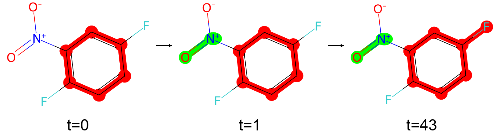
Figure 1: The tokenization of a molecule from Mutag with its SMILES being “c1cc(c(cc1F)[N+](=O)[O-])F”. We color the identified node sets at iteration $t=0,1,43$.

4.2 Algorithm

Given a collection of graphs $D=\{G_{i}=(V_{i},E_{i})\}_{i=1}^{|D|}$, at each iteration $t$, our algorithm aims to tokenize each graph $G^{t-1}_{i}$ into a collection of node sets $\mathcal{V}_{i}^{t}=\{N_{j}^{t}|N_{j}^{t}\in 2^{V_{i}}\}$, where $2^{V_{i}}$ denotes the power set over $V_{i}$ and each node set $N_{j}^{t}$ is viewed as a hypernode, and constructs the next tokenized graph as $G_{i}^{t}=(\mathcal{V}_{i}^{t},E_{i}^{t})$, with $E_{i}^{t}=\{(N_{j}^{t},N_{k}^{t})|\exists v_{m}\in N_{j}^{t},v_{n}\in N_{k}^{t},(v_{m},v_{n})\in E_{i}\}$. A visualization of the tokenization process of our algorithm is presented in Figure 1.

Algorithm 1 shows the proposed GraphBPE, which consists of a preprocessing stage and the tokenization stage. We use $\mathcal{G}$ to denote a general space for graphs, $\mathcal{T}$ to represent the space for different types of topology (e.g., rings), and $\mathcal{S}$ as the space for text strings. We explain the functions used in Algorithm 1 in detail as follows.

• Find()$:\mathcal{G}\times\mathcal{T}\rightarrow 2^{V}$, a function that finds a certain topology $\tau\in\mathcal{T}$ of a graph $G=(V,E)\in\mathcal{G}$, and returns the node set $N^{\tau}\in 2^{V}$ presenting that topology. We abuse the notation of $2^{V}$ which represents the power set of a specific vertex set $V$ henceforth.

• Context()$:\mathcal{G}\times 2^{V}\rightarrow\mathcal{S}$, a function that contextualizes a node set $N^{\tau}\in 2^{V}$ of a graph $G=(V,E)$, mapping it to a identifiable string $s\in\mathcal{S}$.

• Contract()$:\mathcal{G}\times 2^{V}\times\mathcal{S}\rightarrow\mathcal{G}$, a function that contracts a graph $G=(V,E)\in\mathcal{G}$ on a node set $N\in 2^{V}$ and its identifiable string $s\in\mathcal{S}$, and returns a new graph $G^{\prime}=(V^{\prime},E^{\prime})\in\mathcal{G}$ with $N$ being its hypernode, and construct the edge set $E^{\prime}$ such that $E^{\prime}=\{(N,N^{\prime})|\exists v_{m}\in N,v_{n}\in N^{\prime},(v_{m},v_{n})\in E\}$.

• S${}_{\texttt{map}}$()$:\mathcal{S}\times\mathcal{G}\rightarrow 2^{V}$, a function that keeps track of the mapping between a graph $G=(V,E)\in\mathcal{G}$, an identifiable string $s\in\mathcal{S}$ and the corresponding node set $N\in 2^{V}$.

Algorithm 1 GraphBPE

  Input: a collection of graphs $D=\{G_{i}\}_{i=1}^{|D|}$, the number of iterations $T$, a topology identifier Find()$:\mathcal{G}\times\mathcal{T}\rightarrow 2^{V}$, a contextualizer Context()$:\mathcal{G}\times 2^{V}\rightarrow\mathcal{S}$, a structure contractor Contract()$:\mathcal{G}\times 2^{V}\times\mathcal{S}\rightarrow\mathcal{G}$, a frequency recorder Counter()$:\mathcal{S}\rightarrow\mathbb{Z}^{+}$, a structure mapper S${}_{\texttt{map}}$()$:\mathcal{S}\times\mathcal{G}\rightarrow 2^{V}$, and a specific topology $\tau\in\mathcal{T}$ for preprocessing

  Output: the tokenized datasets $D^{0},D^{1},...,D^{T}$

  $D^{0}\leftarrow\{\}$

  # preprocessing

  for $G_{i}$ in $D$ do

     if $\mathcal{T}=\emptyset$ then

        $D^{0}\leftarrow D^{0}\cup\{G_{i}\}$

     else

        $\mathcal{V}_{i}^{\tau}\leftarrow\texttt{Find($G_{i},\tau$)}$

        $s_{i}^{\tau}\leftarrow\texttt{Context($G_{i}^{t},\mathcal{V}_{i}^{\tau}$)}$

        $D^{0}\leftarrow D^{0}\cup\{G_{i}^{0}:=\texttt{Contract($G_{i},\mathcal{V}_{i}^{\tau},s_{i}^{\tau}$)}\}$

     end if

  end for

  # tokenization

  $t\leftarrow 0$

  repeat

     $D^{t+1}\leftarrow\{\}$

     $\texttt{Counter()}\leftarrow\{\}$

     for $G_{i}^{t}(V_{i}^{t},E_{i}^{t})$ in $D^{t}$ do

        for $e$ in $E_{i}^{t}$ do

           $s\leftarrow\texttt{Context($G_{i}^{t},e$)}$

           $\texttt{Counter($s$)}\leftarrow\texttt{Counter($s$)}+1$

           $\texttt{S${}_{\texttt{map}}$($s,G^{t}_{i}$)}\leftarrow e$

        end for

     end for

     $s^{*}=\underset{s^{\prime}}{\arg\max\,}\texttt{Counter($s^{\prime}$)}$

     for $G_{i}^{t}(V_{i}^{t},E_{i}^{t})$ in $D^{t}$ do

        $e\leftarrow\texttt{S${}_{\texttt{map}}$($s^{*},G^{t}_{i}$)}$

        $G_{i}^{t+1}\leftarrow\texttt{Contract($G_{i}^{t},e,s^{*}$)}$

        $D^{t+1}\leftarrow D^{t+1}\cup\{G_{i}^{t+1}\}$

     end for

     $t\leftarrow t+1$

  until $t>T$

Algorithm 2 Contextualizer

  Input: a graph $G=(V,E)$, a set of nodes $V_{c}\in 2^{V}$, a name mapper N${}_{\texttt{map}}$()$:V\times 2^{V}\rightarrow\mathcal{S}$

  Output: a string representation $s$ for $V_{c}$

  # initialize $s$ to be an empty list

  $s\leftarrow[\,\,]$

  for $v$ in $V_{c}$ do

     $s\leftarrow s+\texttt{N${}_{\texttt{map}}$($v,\mathcal{N}(v)$)}$

  end for

  $s\leftarrow\texttt{Sort($s$)}$

  $s\leftarrow\texttt{Concat($s$)}$

Preprocessing. Given a topology $\tau$ (e.g., ring or clique) of interest, we first preprocess the dataset $D$ by contracting the structure $\tau$ for each graph. Specifically, after the node sets for $\tau$ in $G$ are identified by Find(), we contract $G$ into a new graph $G^{0}$ with Contract(), based on the node sets and their contextualized representations. In practice, we only consider $\tau$ being rings or cliques, and $\tau=\emptyset$ means the preprocessing is omitted.

Tokenization. Given a graph $G_{i}^{t-1}\in D^{t-1}$, whose vertices are node sets in $2^{V_{i}}$, we aim to contract $G_{i}^{t-1}$ and build $D^{t}$ following a “count-and-merge” paradigm similar to BPE (as illustrated in Table 1). Specifically, node pairs (i.e., edges) in graphs are the natural analog of paired tokens in texts, and GraphBPE first contextualizes each edge in $D^{t-1}$ into an identifiable string using Context(), and counts its frequency, recorded with S${}_{\texttt{map}}$(). The mostly co-occurred node pair, represented by $s^{*}$, is then selected to merge, where we iterate $D^{t-1}$ again to contract graphs that contain the identification $s^{*}$, and construct $D^{t}$ for the next round of tokenization.

We provide an example implementation of Context() in Algorithm 2. Despite the resemblance between edges and token pairs, one should note that edges in GraphBPE should be treated orderless, meaning as long as two edges contain the same two identifiable strings, they should be viewed as the same (e.g., “$s_{1}\text{-}s_{2}$” is the same as “$s_{2}\text{-}s_{1}$”), which is different from BPE on texts, where the token pairs are order-sensitive (e.g., “lo” is different from “ol”). By customizing the contextualizer, GraphBPE can produce different tokenization strategies, and we present a detailed discussion on how it connects GraphBPE with other tokenization algorithms in Appendix B.
Note that the tokenized graph $G^{t}=(V^{t},E^{t})$ produced by GraphBPE can be viewed as both a simple graph and a hypergraph. Since $V^{t}\subseteq 2^{V}$ and $E^{t}$ is constructed by Contract() such that $G^{t}$ and $G$ have the same number of connected components, with the (untokenized) simple graph being $G=(V,E)$, a simple graph can be derived from $G^{t}$, with each vertex defined by the node ensemble of vertices of $G^{t}$, and its topology defined by $E^{t}$. Naturally, $G^{t}$ defines a hypergraph with hyperedges specified by $V^{t}$ and $E$, where for vertex $v_{s}\in V^{t},|v_{s}|=1$ that remains a single node from $V$, we construct the hyperedges based on the edges $(v_{s},v_{n})\in E,v_{n}\in\mathcal{N}(v_{s})$.

5 Experiment

In this section, we introduce the datasets, tokenization methods for comparison, and models for simple graphs and hypergraphs, and then present the experiment results.

5.1 Dataset

We conduct experiments on graph-level classification and regression datasets, and show their statistics in Table 3. We detail the train-validation-test split in Appendix A.
Classification For graph classification tasks, we choose Mutag, Enzymes, and Proteins from the TUDataset (Morris et al., 2020). Mutag is for binary classification where the goal is to predict the mutagenicity of compounds. Enzymes is a multi-class dataset that focuses on classifying a given enzyme into 6 categories, and Proteins aims to classify whether a protein structure is an enzyme or not.

dataset	# molecule	# class	label distri.	# node type
Mutag	188	2	125:63	7
Enzymes	600	6	balanced	3
Proteins	1113	2	450:663	3
Freesolv	642	1	none	9
Esol	1128	1	none	9
Lipophilicity	4200	1	none	9

Table 3: The statistics of different datasets, where label distri. stands for label distribution. The 1st and 2nd blocks are for graph classification and regression, respectively.

Regression For graph regression tasks, we use Freesolv, Esol, and Lipophilicity from the MoleculeNet (Wu et al., 2018), where Freesolv aims to predict free energy of small molecules in water, Esol targets at predicting water solubility for common organic small molecules, and Lipophilicity focuses on octanol/water distribution coefficient.

Figure 2: Results of a 3-layer GCN, GAT, GIN, and GraphSAGE with a learning rate of 0.01 and a hidden size of 32 on Mutag, Enzymes, and Proteins (1st, 2nd, 3rd row, respectively), with accuracy the higher the better. The x-axis denotes the number of tokenization steps in our GraphBPE algorithm. We plot $\mu\pm\sigma$ over 5 runs for each configuration.

Figure 3: Results of a 3-layer HyperConv, HGNN++, and HNHN (1st, 2nd, 3rd row, respectively) with a learning rate of {0.01, 0.001} and a hidden size of {32, 64} on Freesolv, with RMSE the lower the better. The x-axis denotes the number of tokenization steps in our GraphBPE algorithm. We plot $\mu\pm\sigma$ over 5 runs for GraphBPE, Centroid, and omit $\pm\sigma$ for Chem, H2g for better visualization.

5.2 Tokenization

Given a simple graph $G=(V,E)$, GraphBPE translates it into another graph $G^{\prime}$ whose vertices are node sets in $2^{V}$, which can be then used to construct a hypergraph as defined in Section 3.2. We introduce three other hypergraph construction strategies as follows.
Centroid Following Feng et al. (2019), we construct the hyperedges by choosing each vertex together with its 1-hop neighbors. This is domain-agnostic and requires no extra knowledge, and we refer to it as Centroid.
Chemistry-Informed We can construct hyperedges such that the nodes within which represent functional groups (Li et al., 2023). Specifically, we use RDKit (Landrum et al., 2006) to extract functional groups, and construct each hyperedge based on the nodes that belong to the same functional group. For a node that does not belong to any functional groups, we treat its edges as the respective hyperedges. This method requires domain knowledge in chemistry and we refer to it as Chem.
Hyper2Graph Jin et al. (2020) introduce a motif extraction schedule for molecules based on chemistry knowledge and heuristics. We treat the extracted motifs, which are not necessarily meaningful substructures such as functional groups, as a type of tokenization and refer to this method as H2g.

5.3 Model

We choose two types of models for evaluation, with GNN for (untokenized) simple graphs, and graphs tokenized by GraphBPE at each iteration, and HyperGNN for hypergraphs defined by the tokenization of GraphBPE at each iteration, and constructed by other algorithms. We detail the model implementations in Appendix A.
GNN We choose GCN (Kipf & Welling, 2017), GAT (Veličković et al., 2018), GIN (Xu et al., 2019), and GraphSAGE (Hamilton et al., 2018) for (untokenized) simple graphs and graphs specified by the tokenization of GraphBPE at each iteration.
HyperGNN For hypergraphs constructed by GraphBPE and other tokenization methods, we choose HyperConv (Bai et al., 2020), HGNN++ (Gao et al., 2023), which shows improved performances in metrics and standard deviation over HGNN (Feng et al., 2019) in our preliminary study, and HNHN (Dong et al., 2020) as our three backbones.

5.4 Result

We present experiment results on both classification datasets, with accuracy reported, and regression datasets, with RMSE reported, as suggested by Wu et al. (2018), where for each configuration we run experiments 5 times and report the mean and standard deviation of the metrics. For GraphBPE, we present the results on preprocessing with 100 steps of tokenization. We also report the results on the number of times GraphBPE is statistically (with p-value $<0.05$) / numerically better / the same / worse compared with the baselines. Due to space limits, we present the rest of the results in Appendix C.
GNN We present the test accuracy for 3-layer GNNs on Mutag, Enzymes, and Proteins in Figure 2 and the results on performance comparison in Table 4.

In Figure 2, we can observe that on the Mutag dataset, GraphBPE performs better in general across different GNN architectures, especially for GCN and GraphSAGE, where at different time steps our algorithm consistently outperforms the untokenized molecular graphs in terms of mean$\pm$std. This suggests that tokenization could potentially help the performance of GNNs on molecular graphs. For Enzymes and Proteins, GrapgBPE does not consistently perform better than untokenized graphs, where both the tokenization step and the choice of the model will affect the accuracy. For example, approximately the first 20 tokenization steps are favored by GAT on both Enzymes and Proteins, and the performance begins to degenerate as the tokenization step increases, while for GIN on Enzymes, our algorithm is outperformed in all time steps.

dataset	strategy	GCN	GAT	GIN	GraphSAGE
Mutag	p-value	93:8:0	17:84:0	1:100:0	96:5:0
	metric	101:0:0	99:0:2	78:2:21	101:0:0
Enzymes	p-value	0:101:0	0:100:1	0:54:47	0:101:0
	metric	66:1:34	38:0:63	0:0:101	37:1:63
Proteins	p-value	1:100:0	1:94:6	16:84:1	0:101:0
	metric	98:0:3	32:1:68	95:0:6	16:0:85

Table 4: Performance comparison on the accuracy of classification datasets for 3-layer GNNs with a learning rate of 0.01 and a hidden size of 32. For each triplet $a$:$b$:$c$, $a,b,c$ are the number of times GraphBPE is better / the same / worse compared with (untokenized) simple graphs. “p-value” stands for comparison based on p-value $<0.05$ from t-test, and “metric” means numerical comparison of the metric values, where best within the triplet is bold.

In terms of metric value comparison and statistical significance, we can observe from Table 4 that most of the time we can outperform untokenized graphs in terms of average accuracy, while performing as least the same under the lens of significance tests (e.g., t-test with a p-value $<$ 0.05), which aligns with our findings from Figure 2.

In general, we can observe that GraphBPE performs less satisfyingly as the dataset size increases, we suspect this might be because the vocabulary to be mined on large datasets is complex and diverse, such that the number of (limited) tokenization steps would affect the performance; thus, more tokenization steps might be favored to achieve better results on large datasets.
HyperGNN We present the test RMSE for 3-layer hyperGNNs on Freesolv over different configurations (learning rate $\times$ hidden size) in Figure 3 and the results on performance comparison for one configuration in Table 5.

method	strategy	HyperConv	HGNN++	HNHN
Centroid	p-value	0:101:0	0:101:0	1:100:0
	metric	26:0:75	38:0:63	75:0:26
Chem	p-value	0:99:2	0:97:4	0:100:1
	metric	28:0:73	5:0:96	71:0:30
H2g	p-value	1:100:0	0:99:2	0:101:0
	metric	60:0:41	35:0:66	83:0:18

Table 5: Performance comparison on the RMSE of 3-layer HyperGNNs with a learning rate of 0.01 and a hidden size of 32 on Freesolv. For each triplet $a$:$b$:$c$, $a,b,c$ are the number of times GraphBPE is better / the same / worse compared with other tokenization methods. “p-value” stands for comparison based on p-value $<0.05$ from t-test, and “metric” means numerical comparison of the metric values, where best within the triplet is bold.

As shown in Figure 3, both learning rate and model architectures can largely affect the test performance, and no tokenization methods can perform universally well across different configurations. In terms of the average performance, there generally exists some steps for GraphBPE in different configurations, which have the lowest RMSE compared with other tokenization methods. However, there is yet no method that can determine such “optimal” tokenization steps ahead of training.

We choose the configuration with a learning rate of 0.01 and a hidden size of 32 to further conduct performance comparison, as it achieves lower RMSE across different models. As detailed in Table 5, we can observe that model architectures will affect the performance, and again, no tokenization method is the best among different configurations. For metric value comparison, GraphBPE shows good performance on HNHN and frequently outperforms other tokenization methods, while less is less satisfying on other models. However, we can observe that there always exists some steps (i.e., the number of times GraphBPE is better compared with other tokenization methods) that GraphBPE achieves a lower RMSE, similar to the findings from Figure 3. In terms of the comparison based on p-values, our method performs the same compared with the baselines most of the time, unlike on Mutag where we can demonstrate statistical significance. We suspect that this might be because tokenization is in general less effective for regression tasks, which is supported by the results in Appendix C.

In general, we can observe that the choice of tokenization methods will largely affect the performance of hyperGNNs, suggesting that a well-designed hypergraph construction strategy would benefit hyperGNNs on molecular graphs. Although GraphBPE often has steps that achieve a smaller RMSE against the baselines for different configurations, it in general shows limited improvement for regression tasks compared to classification tasks.

6 Conclusion

In this work, we explore how tokenization would help molecular machine learning on classification and regression tasks, and propose GraphBPE, a count-and-merge algorithm that tokenize a simple graph into node sets, which are later used to construct a new (simple) graph or a hypergraph. Our experiment across various datasets and models suggests that tokenization will affect the test performance, and our proposed GraphBPE tends to excel on small classification datasets, given a limited number of tokenization steps.

We explore the simple idea of how different views of molecular graphs would benefit graph-level tasks, and we hope our results can inspire more discussions and attract attention to the data preprocessing schedules for molecule machine learning, which is less studied compared with innovations on models and benchmarks.

Limitation

Types of Tokenization We include two types of tokenization baselines where one is based on chemistry knowledge and the other is based on pre-defined rules. However, there exist more sophisticated tokenization methods, such as deriving tokenization rules from an off-the-shelf GNN, which are not discussed in this work.

Types of Task & Dataset We focus on graph-level tasks and exclude node-level tasks. For the classification and regression task, although we include three datasets for each and consider both binary and multi-class classification datasets, the size of our datasets (e.g., $\sim 10^{3}$) is relatively small compared with those usually used for molecular graph pre-training (e.g., $\sim 10^{6}$).

Impact Statement

This paper presents work whose goal is to advance the field of Machine Learning. There are many potential societal consequences of our work, none of which we feel must be specifically highlighted here.

Appendix A Implementation

For all the models, we use {1, 2, 3}-layer architecture with a hidden size of {32, 64} and a learning rate of {0.01, 0.001}. For both classification and regression tasks, we apply a 1-layer MLP with a dropout rate of 0.1. We use a batch size of the form $2^{N}\cdot 10^{M}$ where $N,M$ are chosen such that the batch size can approximately cover the entire training set, and we further apply BatchNorm (Ioffe & Szegedy, 2015) to stabilize the training. We train the model for 100 epochs, and report the mean $\mu$ and standard deviation $\sigma$ over 5 runs for the test performance on the model with the best validation performance.

For datasets with a size smaller than 2000, we adopt a train-validation-test split of 0.6/0.2/0.2, and use 0.8/0.1/0.1 for larger datasets. We ignore the edge features and use the one-hot encodings as the node features. For the tokenized graphs from GraphBPE, we use the summation of the node features as the representation for that hypernode for our experiments on GNNs. For classification datasets, we make the validation and test set as balanced as possible, as suggested in our preliminary study, that using a random split validation set might favor models that are not trained at all (e.g., models always predict positive for binary classification task). For regression datasets, we follow Wu et al. (2018) and use random split. For Mutag, Freesolv, Esol, and Lipophilicity, we set the topology to be contracted as rings in the preprocessing stage, and we set that for Enzymes and Proteins as cliques.

Note that from untokenized graphs to the last iteration $T$, we can track how the nodes merge into node sets in the graph and thus develop a tokenization rule for unseen graphs. However, for simplicity and efficiency, we first tokenize the entire dataset before we split them into train/validation/test sets. Our code is available at https://github.com/A-Chicharito-S/GraphBPE.

Appendix B Discussion on Contextualizer

Algorithm 3 PSE-Contextualizer

  Input: a graph $G=(V,E)$, a set of nodes $V_{c}\in 2^{V}$, a name mapper N${}_{\texttt{map}}$()$:V\times 2^{V}\rightarrow\emptyset$

  Output: a string representation $s$ for $V_{c}$

  # initialize $s$ to be an empty list

  $s\leftarrow[\,\,]$

  for $v$ in $V_{c}$ do

     $s\leftarrow s+\texttt{N${}_{\texttt{map}}$($v,\mathcal{N}(v)$)}$

  end for

  $s\leftarrow\texttt{Sort($s$)}$

  $s\leftarrow\texttt{Concat($s$)}$

For the Principal Subgraph Extraction (PSE) algorithm proposed by Kong et al. (2022), we can recover it from GraphBPE by skipping the preprocessing stage, while setting the contextualizer as Algorithm 3. The only difference between the PSE contextualizer and ours is that in Algorithm 3, the name mapper N${}_{\texttt{map}}$() returns an empty string for any node sets, while ours returns the string representation for the neighborhood, meaning PSE does not take the neighbors/context into consideration during tokenization. For the Connection-Aware Motif Mining algorithm proposed by Geng et al. (2023), where the connection among the nodes is considered to mine common substructures (e.g., as illustrated in Figure 2 of Geng et al. (2023), 3 hypernodes can be contracted at a time), we can recover it by increasing the number of tokenization steps, which mitigates the fact that GraphBPE always select one pair of nodes to contract.

Note that by customizing the N${}_{\texttt{map}}$() function, we can further introduce external knowledge (e.g., include information about the chemistry properties), and constraints (e.g., limit the maximum size of the node set) in the tokenization process, and potentially extend our algorithm for non-molecular graphs that do not necessarily share common node types across different graphs, where instead of return the string representation of the neighborhood, N${}_{\texttt{map}}$() can give out the structural information (e.g., the degree of the node) that reveals the neighborhood to facilitate tokenization.

Appendix C Result

We include the visualization of the test performance, and the performance comparison based on p-value and metric-value for Mutag, Enzymes, Proteins, Freesolv, Esol, and Lipophilicity in Section C.1,  C.2,  C.3,  C.4,  C.5 and  C.6. For better visualization, we plot both the mean and the standard deviation as $\mu\pm\sigma$ for our experiments on GNNs, and exclude the standard deviation for the Chem, H2g baselines on HyperGNNs. For the performance comparison, we use the triplet $a:b:c$ to denote the number of times our algorithms are better / the same / worse compared with the baseline, and use red to mark the best within the triplet based on p-value comparison, and black to mark that for metric value comparison. We can observe that in general, given the 100 tokenization steps, GraphBPE tend to perform well on small datasets, which we suspect is due to the reason that larger datasets contain richer substructures to learn; thus, may need more tokenization rounds. Compared with regression tasks, GraphBPE tends to provide more boosts for classification tasks.

C.1 Mutag

For GNNs, we include the performance comparison results in Table 10, and the visualization over different tokenization steps in Figure 4,  5,  6, and  7 for GCN, GAT, GIN, and GraphSAGE.

For HyperGNNs, we include the performance comparison results in Table 20, and the visualization over different tokenization steps in Figure 8,  9, and  10 for HyperConv, HGNN++, and HNHN.

learning rate		$10^{-2}$		$10^{-3}$
hidden size		$h=32$	$h=64$	$h=32$	$h=64$
$L={1}$	p-value	86:15:0	93:8:0	37:64:0	95:6:0
	metric	101:0:0	101:0:0	97:1:3	101:0:0
$L={2}$	p-value	101:0:0	89:12:0	1:100:0	11:90:0
	metric	101:0:0	101:0:0	91:0:10	91:2:8
$L={3}$	p-value	93:8:0	100:1:0	1:100:0	36:65:0
	metric	101:0:0	101:0:0	77:4:20	101:0:0

Table 6: Comparison with p-/metric value of GCN

learning rate		$10^{-2}$		$10^{-3}$
hidden size		$h=32$	$h=64$	$h=32$	$h=64$
$L={1}$	p-value	0:97:4	0:19:82	17:84:0	2:99:0
	metric	6:1:94	0:0:101	101:0:0	94:0:7
$L={2}$	p-value	0:18:83	0:16:85	0:101:0	0:93:8
	metric	0:0:101	1:0:100	67:0:34	0:0:101
$L={3}$	p-value	1:100:0	2:99:0	2:98:1	0:101:0
	metric	78:2:21	84:4:13	74:0:27	68:4:29

Table 7: Comparison with p-/metric value of GIN

learning rate		$10^{-2}$		$10^{-3}$
hidden size		$h=32$	$h=64$	$h=32$	$h=64$
$L={1}$	p-value	84:17:0	99:2:0	58:43:0	11:90:0
	metric	101:0:0	101:0:0	98:1:2	96:1:4
$L={2}$	p-value	101:0:0	97:4:0	63:38:0	29:72:0
	metric	101:0:0	101:0:0	100:0:1	100:0:1
$L={3}$	p-value	17:84:0	57:44:0	45:56:0	73:28:0
	metric	99:0:2	101:0:0	101:0:0	100:0:1

Table 8: Comparison with p-/metric value of GAT

learning rate		$10^{-2}$		$10^{-3}$
hidden size		$h=32$	$h=64$	$h=32$	$h=64$
$L={1}$	p-value	100:1:0	101:0:0	58:43:0	85:16:0
	metric	101:0:0	101:0:0	97:0:4	101:0:0
$L={2}$	p-value	101:0:0	99:2:0	89:12:0	36:65:0
	metric	101:0:0	101:0:0	101:0:0	101:0:0
$L={3}$	p-value	96:5:0	79:22:0	100:1:0	101:0:0
	metric	101:0:0	101:0:0	101:0:0	101:0:0

Table 9: Comparison with p-/metric value of GraphSAGE

Table 10: Performance comparison on accuracy with p-value $<0.05$ and metric value on Mutag. For each triplet $a$:$b$:$c$, $a,b,c$ denote the number of times GraphBPE is statistically/numerically better/the same/worse compared with (untokenized) simple graph.

Figure 4: Results of GCN on Mutag, with accuracy the higher the better

Figure 5: Results of GAT on Mutag, with accuracy the higher the better

Figure 6: Results of GIN on Mutag, with accuracy the higher the better

Figure 7: Results of GraphSAGE on Mutag, with accuracy the higher the better

learning rate		$10^{-2}$		$10^{-3}$
hidden size		$h=32$	$h=64$	$h=32$	$h=64$
$L={1}$	p-value	12:88:1	5:89:7	44:57:0	51:50:0
	metric	82:2:17	56:5:40	101:0:0	100:0:1
$L={2}$	p-value	0:100:1	0:91:10	0:101:0	47:54:0
	metric	26:2:73	17:0:84	21:3:77	98:2:1
$L={3}$	p-value	0:99:2	40:61:0	4:97:0	0:101:0
	metric	58:5:38	96:2:3	59:0:42	17:1:83

Table 11: Centroid on HyperConv

learning rate		$10^{-2}$		$10^{-3}$
hidden size		$h=32$	$h=64$	$h=32$	$h=64$
$L={1}$	p-value	18:82:1	16:83:2	10:91:0	3:96:2
	metric	84:1:16	89:0:12	84:3:14	71:5:25
$L={2}$	p-value	8:92:1	2:97:2	4:97:0	0:87:14
	metric	76:4:21	59:1:41	83:0:18	23:1:77
$L={3}$	p-value	4:95:2	31:70:0	0:94:7	0:100:1
	metric	73:0:28	93:1:7	27:1:73	29:6:66

Table 12: Chem on HyperConv

learning rate		$10^{-2}$		$10^{-3}$
hidden size		$h=32$	$h=64$	$h=32$	$h=64$
$L={1}$	p-value	7:92:2	7:89:5	1:94:6	0:93:8
	metric	75:2:24	56:5:40	42:0:59	12:2:87
$L={2}$	p-value	7:91:3	3:94:4	0:95:6	1:92:8
	metric	70:4:27	56:3:42	3:0:98	35:3:63
$L={3}$	p-value	1:96:4	34:67:0	1:85:15	3:97:1
	metric	33:1:67	93:1:7	28:0:73	75:5:21

Table 13: H2g on HyperConv

learning rate		$10^{-2}$		$10^{-3}$
hidden size		$h=32$	$h=64$	$h=32$	$h=64$
$L={1}$	p-value	1:100:0	9:88:4	35:66:0	0:96:5
	metric	39:3:59	70:2:29	99:1:1	39:6:56
$L={2}$	p-value	1:100:0	39:62:0	0:93:8	2:99:0
	metric	57:5:39	97:1:3	11:0:90	77:1:23
$L={3}$	p-value	25:76:0	0:100:1	1:95:5	0:101:0
	metric	98:0:3	51:5:45	54:3:44	27:1:73

Table 14: Centroid on HGNN++

learning rate		$10^{-2}$		$10^{-3}$
hidden size		$h=32$	$h=64$	$h=32$	$h=64$
$L={1}$	p-value	0:78:23	7:85:9	0:98:3	2:99:0
	metric	7:0:94	51:5:45	18:2:81	69:4:28
$L={2}$	p-value	4:93:4	7:93:1	1:94:6	0:92:9
	metric	45:5:51	52:3:46	54:3:44	12:0:89
$L={3}$	p-value	23:78:0	1:98:2	0:83:18	0:100:1
	metric	91:0:10	49:2:50	13:4:84	18:0:83

Table 15: Chem on HGNN++

learning rate		$10^{-2}$		$10^{-3}$
hidden size		$h=32$	$h=64$	$h=32$	$h=64$
$L={1}$	p-value	0:87:14	0:91:10	0:89:12	0:79:22
	metric	25:2:74	35:6:60	20:0:81	5:1:95
$L={2}$	p-value	5:96:0	35:66:0	0:99:2	0:81:20
	metric	74:5:22	90:0:11	39:5:57	5:2:94
$L={3}$	p-value	4:97:0	12:89:0	0:99:2	0:101:0
	metric	83:3:15	80:3:18	8:2:91	40:7:54

Table 16: H2g on HGNN++

learning rate		$10^{-2}$		$10^{-3}$
hidden size		$h=32$	$h=64$	$h=32$	$h=64$
$L={1}$	p-value	6:95:0	11:90:0	13:88:0	27:74:0
	metric	93:0:8	76:2:23	79:4:18	99:0:2
$L={2}$	p-value	9:92:0	10:91:0	0:96:5	6:95:0
	metric	84:0:17	94:2:5	38:1:62	75:2:24
$L={3}$	p-value	20:81:0	9:91:1	24:77:0	2:99:0
	metric	100:1:0	70:2:29	101:0:0	61:2:38

Table 17: Centroid on HNHN

learning rate		$10^{-2}$		$10^{-3}$
hidden size		$h=32$	$h=64$	$h=32$	$h=64$
$L={1}$	p-value	19:82:0	39:62:0	9:92:0	2:99:0
	metric	91:2:8	101:0:0	97:0:4	69:4:28
$L={2}$	p-value	9:91:1	9:92:0	0:101:0	0:100:1
	metric	83:1:17	99:0:2	62:6:33	27:0:74
$L={3}$	p-value	3:98:0	11:90:0	16:85:0	67:34:0
	metric	80:3:18	98:0:3	96:1:4	101:0:0

Table 18: Chem on HNHN

learning rate		$10^{-2}$		$10^{-3}$
hidden size		$h=32$	$h=64$	$h=32$	$h=64$
$L={1}$	p-value	13:88:0	16:85:0	17:84:0	2:98:1
	metric	93:0:8	83:3:15	92:0:9	51:4:46
$L={2}$	p-value	17:83:1	7:94:0	0:97:4	3:95:3
	metric	90:3:8	89:0:12	7:0:94	39:3:59
$L={3}$	p-value	11:89:1	28:73:0	0:93:8	14:87:0
	metric	85:1:15	99:0:2	32:2:67	93:0:8

Table 19: H2g on HNHN

Table 20: Performance comparison on accuracy with p-value $<0.05$ and metric value on Mutag. For each triplet $a$:$b$:$c$, $a,b,c$ denote the number of times GraphBPE is statistically/numerically better/the same/worse compared with hypergraphs constructed by Method on Model (e.g., “Centroud on HyperConv” means comparing GraphBPE with Centroid on the HyperConv model).

Figure 8: Results of HyperConv on Mutag, with accuracy the higher the better

Figure 9: Results of HGNN++ on Mutag, with accuracy the higher the better

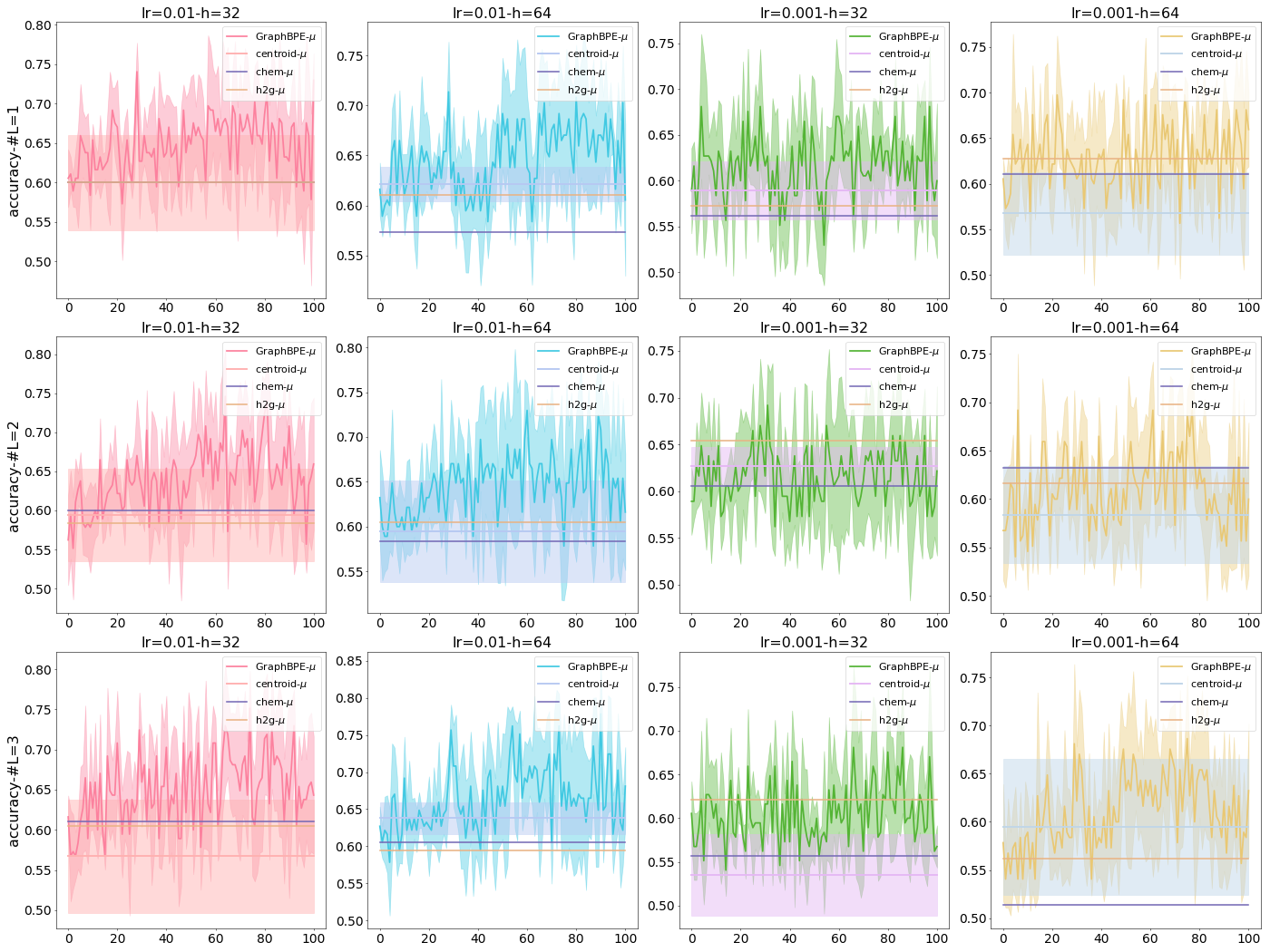
Figure 10: Results of HNHN on Mutag, with accuracy the higher the better

C.2 Enzymes

For GNNs, we include the performance comparison results in Table 25, and the visualization over different tokenization steps in Figure 11,  12,  13, and  14 for GCN, GAT, GIN, and GraphSAGE.

For HyperGNNs, we include the performance comparison results in Table 29, and the visualization over different tokenization steps in Figure 15,  16, and  17 for HyperConv, HGNN++, and HNHN.

learning rate		$10^{-2}$		$10^{-3}$
hidden size		$h=32$	$h=64$	$h=32$	$h=64$
$L={1}$	p-value	2:99:0	2:99:0	1:100:0	41:60:0
	metric	66:0:35	100:0:1	77:0:24	101:0:0
$L={2}$	p-value	0:101:0	0:101:0	13:88:0	0:99:2
	metric	91:2:8	39:1:61	101:0:0	49:0:52
$L={3}$	p-value	0:101:0	3:98:0	0:101:0	2:96:3
	metric	66:1:34	96:0:5	63:0:38	29:3:69

Table 21: Comparison with p-/metric value of GCN

learning rate		$10^{-2}$		$10^{-3}$
hidden size		$h=32$	$h=64$	$h=32$	$h=64$
$L={1}$	p-value	0:6:95	0:19:82	1:100:0	0:97:4
	metric	0:0:101	0:0:101	94:0:7	15:0:86
$L={2}$	p-value	0:101:0	1:90:10	0:100:1	0:90:11
	metric	18:2:81	35:0:66	12:0:89	4:1:96
$L={3}$	p-value	0:54:47	0:86:15	0:101:0	7:94:0
	metric	0:0:101	2:0:99	37:0:64	82:0:19

Table 22: Comparison with p-/metric value of GIN

learning rate		$10^{-2}$		$10^{-3}$
hidden size		$h=32$	$h=64$	$h=32$	$h=64$
$L={1}$	p-value	0:95:6	0:95:6	9:91:1	3:98:0
	metric	6:0:95	6:0:95	81:0:20	91:1:9
$L={2}$	p-value	11:90:0	1:100:0	2:99:0	2:98:1
	metric	91:0:10	97:0:4	88:1:12	47:2:52
$L={3}$	p-value	0:100:1	0:75:26	1:100:0	0:91:10
	metric	38:0:63	2:0:99	77:1:23	0:0:101

Table 23: Comparison with p-/metric value of GAT

learning rate		$10^{-2}$		$10^{-3}$
hidden size		$h=32$	$h=64$	$h=32$	$h=64$
$L={1}$	p-value	0:101:0	0:100:1	3:98:0	0:99:2
	metric	20:0:81	5:0:96	88:2:11	1:0:100
$L={2}$	p-value	1:100:0	0:101:0	27:74:0	4:97:0
	metric	74:0:27	65:3:33	99:0:2	95:0:6
$L={3}$	p-value	0:101:0	0:93:8	1:100:0	0:101:0
	metric	37:1:63	3:0:98	100:0:1	1:0:100

Table 24: Comparison with p-/metric value of GraphSAGE

Table 25: Performance comparison on accuracy with p-value $<0.05$ and metric value on Enzymes. For each triplet $a$:$b$:$c$, $a,b,c$ denote the number of times GraphBPE is statistically/numerically better/the same/worse compared with (untokenized) simple graph.

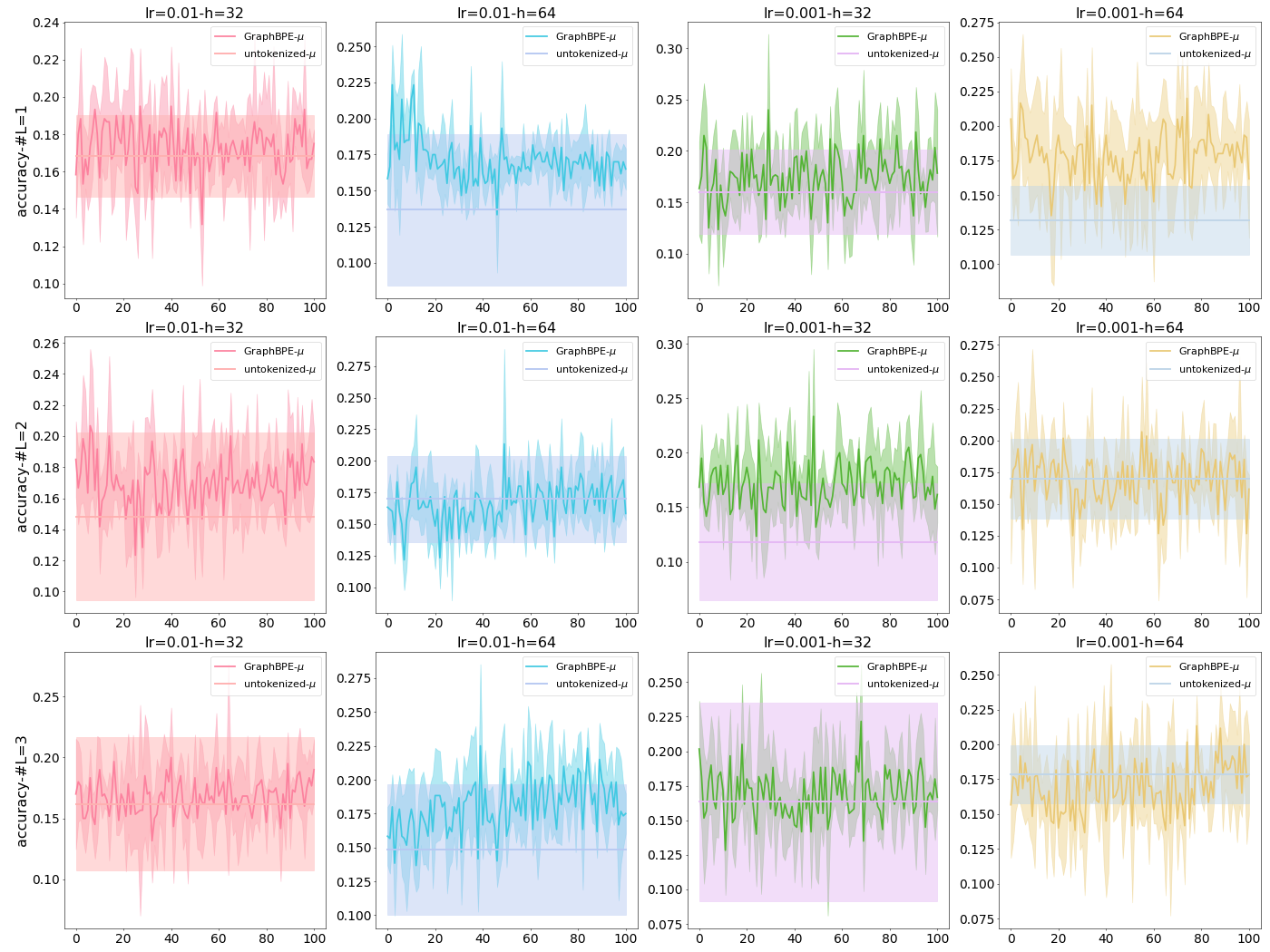
Figure 11: Results of GCN on Enzymes, with accuracy the higher the better

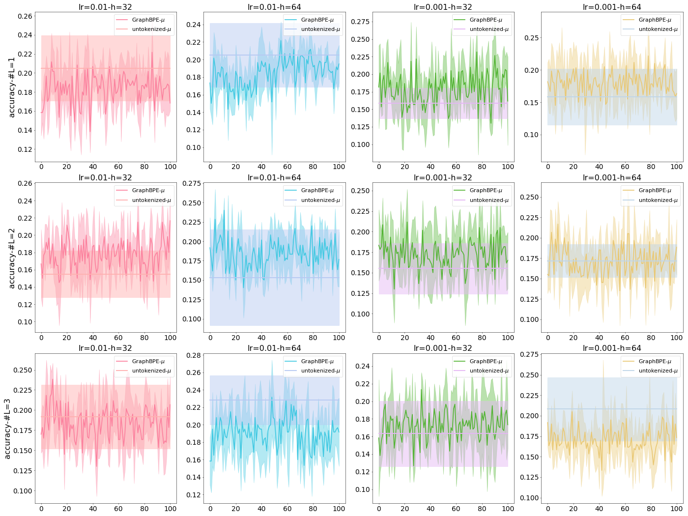
Figure 12: Results of GAT on Enzymes, with accuracy the higher the better

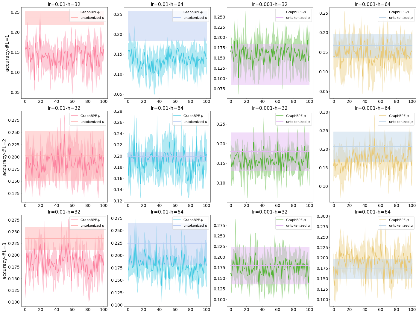
Figure 13: Results of GIN on Enzymes, with accuracy the higher the better

Figure 14: Results of GraphSAGE on Enzymes, with accuracy the higher the better

learning rate		$10^{-2}$		$10^{-3}$
hidden size		$h=32$	$h=64$	$h=32$	$h=64$
$L={1}$	p-value	1:96:4	36:65:0	0:101:0	0:100:1
	metric	52:0:49	101:0:0	45:0:56	20:0:81
$L={2}$	p-value	0:93:8	0:91:10	2:97:2	5:96:0
	metric	12:0:89	0:0:101	42:0:59	79:0:22
$L={3}$	p-value	2:99:0	5:95:1	0:98:3	0:101:0
	metric	82:0:19	72:0:29	16:0:85	81:0:20

Table 26: Centroid on HyperConv

learning rate		$10^{-2}$		$10^{-3}$
hidden size		$h=32$	$h=64$	$h=32$	$h=64$
$L={1}$	p-value	0:101:0	0:100:1	2:99:0	1:100:0
	metric	90:0:11	49:0:52	92:0:9	81:0:20
$L={2}$	p-value	8:93:0	0:101:0	0:96:5	2:99:0
	metric	69:0:32	57:0:44	22:2:77	97:0:4
$L={3}$	p-value	4:97:0	0:94:7	0:101:0	0:100:1
	metric	89:0:12	13:0:88	30:0:71	21:0:80

Table 27: Centroid on HGNN++

learning rate		$10^{-2}$		$10^{-3}$
hidden size		$h=32$	$h=64$	$h=32$	$h=64$
$L={1}$	p-value	3:98:0	0:101:0	1:99:1	1:100:0
	metric	95:0:6	50:1:50	65:0:36	48:0:53
$L={2}$	p-value	0:101:0	0:100:1	0:91:10	0:100:1
	metric	4:0:97	29:0:72	5:0:96	45:0:56
$L={3}$	p-value	0:101:0	22:79:0	8:93:0	6:94:1
	metric	96:0:5	95:0:6	90:0:11	68:1:32

Table 28: Centroid on HNHN

Table 29: Performance comparison on accuracy with p-value $<0.05$ and metric value on Enzymes. For each triplet $a$:$b$:$c$, $a,b,c$ denote the number of times GraphBPE is statistically/numerically better/the same/worse compared with hypergraphs constructed by Method on Model (e.g., “Centroud on HyperConv” means comparing GraphBPE with Centroid on the HyperConv model).

Figure 15: Results of HyperConv on Enzymes, with accuracy the higher the better

Figure 16: Results of HGNN++ on Enzymes, with accuracy the higher the better

Figure 17: Results of HNHN on Enzymes, with accuracy the higher the better

C.3 Proteins

For GNNs, we include the performance comparison results in Table 34, and the visualization over different tokenization steps in Figure 18,  19,  20, and  21 for GCN, GAT, GIN, and GraphSAGE.

For HyperGNNs, we include the performance comparison results in Table 38, and the visualization over different tokenization steps in Figure 22,  23, and  24 for HyperConv, HGNN++, and HNHN.

learning rate		$10^{-2}$		$10^{-3}$
hidden size		$h=32$	$h=64$	$h=32$	$h=64$
$L={1}$	p-value	101:0:0	9:92:0	57:44:0	3:98:0
	metric	101:0:0	97:0:4	101:0:0	88:0:13
$L={2}$	p-value	0:48:53	3:97:1	2:99:0	0:61:40
	metric	0:0:101	64:0:37	89:1:11	0:0:101
$L={3}$	p-value	1:100:0	53:48:0	0:83:18	5:96:0
	metric	98:0:3	99:0:2	3:1:97	99:0:2

Table 30: Comparison with p-/metric value of GCN

learning rate		$10^{-2}$		$10^{-3}$
hidden size		$h=32$	$h=64$	$h=32$	$h=64$
$L={1}$	p-value	3:93:5	0:90:11	53:48:0	29:70:2
	metric	43:0:58	20:0:81	98:0:3	87:1:13
$L={2}$	p-value	6:95:0	15:86:0	88:13:0	2:97:2
	metric	98:0:3	98:0:3	101:0:0	28:4:69
$L={3}$	p-value	16:84:1	3:98:0	11:90:0	8:93:0
	metric	95:0:6	78:1:22	98:1:2	100:0:1

Table 31: Comparison with p-/metric value of GIN

learning rate		$10^{-2}$		$10^{-3}$
hidden size		$h=32$	$h=64$	$h=32$	$h=64$
$L={1}$	p-value	3:98:0	2:96:3	0:81:20	76:25:0
	metric	47:1:53	54:2:45	0:0:101	101:0:0
$L={2}$	p-value	19:78:4	13:88:0	18:83:0	9:92:0
	metric	77:0:24	84:0:17	96:0:5	88:0:13
$L={3}$	p-value	1:94:6	7:92:2	0:81:20	6:95:0
	metric	32:1:68	54:1:46	9:1:91	93:2:6

Table 32: Comparison with p-/metric value of GAT

learning rate		$10^{-2}$		$10^{-3}$
hidden size		$h=32$	$h=64$	$h=32$	$h=64$
$L={1}$	p-value	0:58:43	5:60:36	1:100:0	0:100:1
	metric	10:1:90	19:0:82	84:0:17	6:0:95
$L={2}$	p-value	10:91:0	0:97:4	0:82:19	34:67:0
	metric	91:0:10	35:1:65	5:0:96	97:1:3
$L={3}$	p-value	0:101:0	0:28:73	35:66:0	0:101:0
	metric	16:0:85	0:0:101	99:1:1	61:1:39

Table 33: Comparison with p-/metric value of GraphSAGE

Table 34: Performance comparison on accuracy with p-value $<0.05$ and metric value on Proteins. For each triplet $a$:$b$:$c$, $a,b,c$ denote the number of times GraphBPE is statistically/numerically better/the same/worse compared with (untokenized) simple graph.

Figure 18: Results of GCN on Proteins, with accuracy the higher the better

Figure 19: Results of GAT on Proteins, with accuracy the higher the better

Figure 20: Results of GIN on Proteins, with accuracy the higher the better

Figure 21: Results of GraphSAGE on Proteins, with accuracy the higher the better

learning rate		$10^{-2}$		$10^{-3}$
hidden size		$h=32$	$h=64$	$h=32$	$h=64$
$L={1}$	p-value	0:10:91	0:2:99	2:97:2	1:90:10
	metric	0:0:101	0:0:101	81:1:19	9:0:92
$L={2}$	p-value	0:71:30	0:74:27	0:76:25	0:100:1
	metric	0:0:101	2:0:99	1:0:100	4:0:97
$L={3}$	p-value	0:28:73	0:69:32	0:43:58	0:97:4
	metric	0:0:101	0:0:101	0:0:101	7:0:94

Table 35: Centroid on HyperConv

learning rate		$10^{-2}$		$10^{-3}$
hidden size		$h=32$	$h=64$	$h=32$	$h=64$
$L={1}$	p-value	0:53:48	0:57:44	0:97:4	0:92:9
	metric	0:0:101	1:0:100	19:0:82	9:2:90
$L={2}$	p-value	2:94:5	0:97:4	0:99:2	16:85:0
	metric	30:2:69	14:1:86	16:2:83	101:0:0
$L={3}$	p-value	0:96:5	0:98:3	0:99:2	0:101:0
	metric	4:0:97	48:1:52	29:0:72	94:0:7

Table 36: Centroid on HGNN++

learning rate		$10^{-2}$		$10^{-3}$
hidden size		$h=32$	$h=64$	$h=32$	$h=64$
$L={1}$	p-value	0:80:21	0:71:30	0:91:10	1:86:14
	metric	0:0:101	1:0:100	7:0:94	8:1:92
$L={2}$	p-value	0:100:1	0:76:25	0:101:0	0:101:0
	metric	11:4:86	1:0:100	55:0:46	34:0:67
$L={3}$	p-value	0:101:0	0:94:7	0:95:6	0:86:15
	metric	38:2:61	13:2:86	17:3:81	14:0:87

Table 37: Centroid on HNHN

Table 38: Performance comparison on accuracy with p-value $<0.05$ and metric value on Proteins. For each triplet $a$:$b$:$c$, $a,b,c$ denote the number of times GraphBPE is statistically/numerically better/the same/worse compared with hypergraphs constructed by Method on Model (e.g., “Centroud on HyperConv” means comparing GraphBPE with Centroid on the HyperConv model).

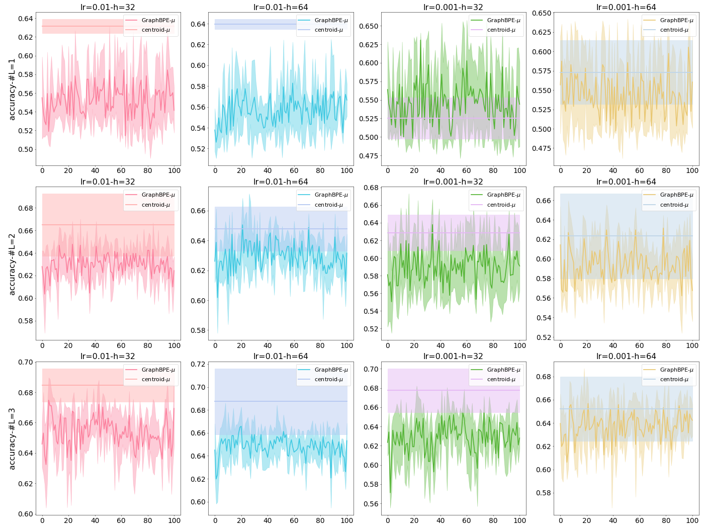
Figure 22: Results of HyperConv on Proteins, with accuracy the higher the better

Figure 23: Results of HGNN++ on Proteins, with accuracy the higher the better

Figure 24: Results of HNHN on Proteins, with accuracy the higher the better

C.4 Freesolv

For GNNs, we include the performance comparison results in Table 43, and the visualization over different tokenization steps in Figure 25,  26,  27, and  28 for GCN, GAT, GIN, and GraphSAGE.

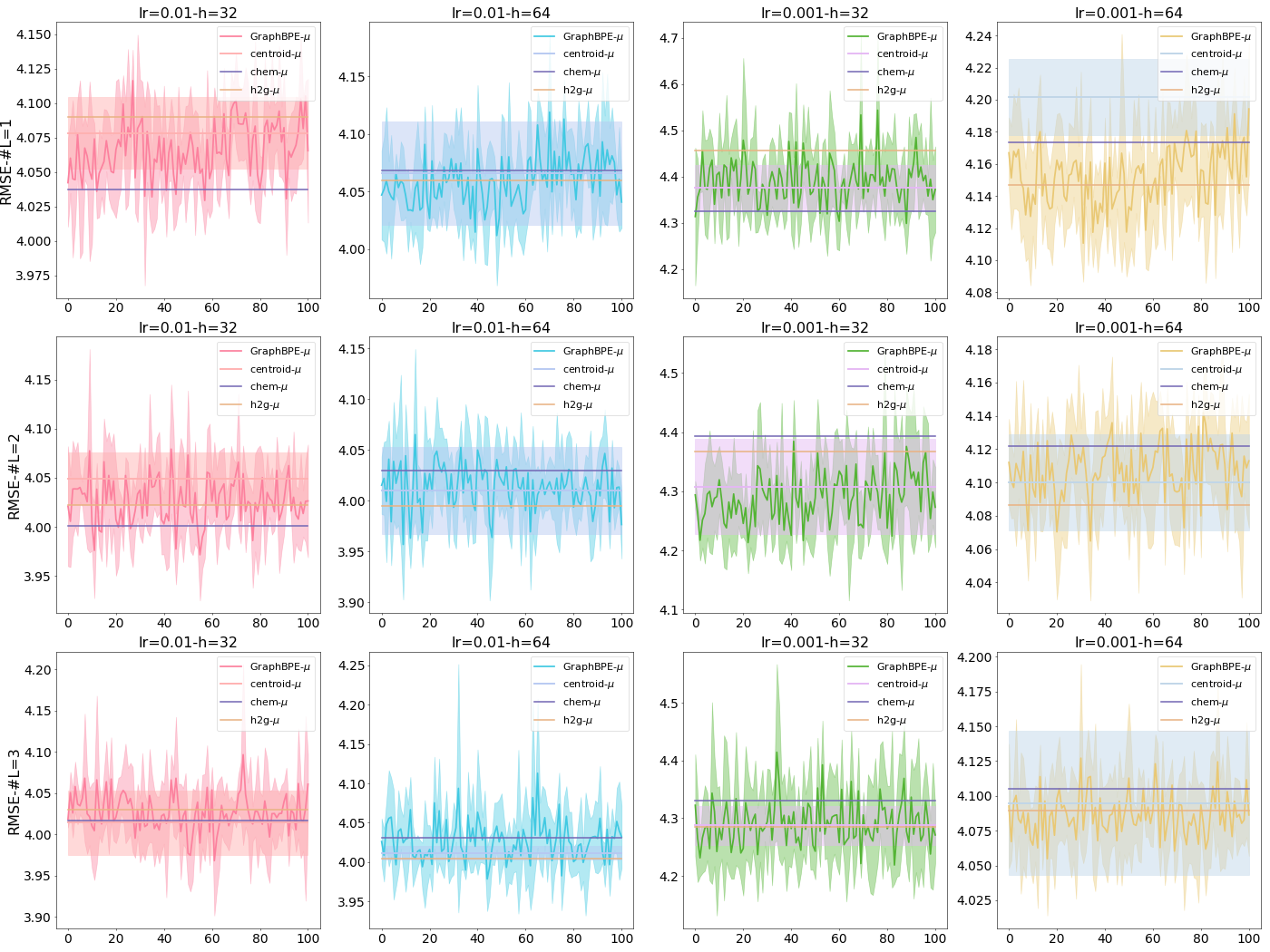
Figure 29: Results of HyperConv on Freesolv, with RMSE the lower the better

For HyperGNNs, we include the performance comparison results in Table 53, and the visualization over different tokenization steps in Figure 29,  30, and  31 for HyperConv, HGNN++, and HNHN.

learning rate		$10^{-2}$		$10^{-3}$
hidden size		$h=32$	$h=64$	$h=32$	$h=64$
$L={1}$	p-value	0:46:55	0:56:45	0:3:98	0:0:101
	metric	0:0:101	0:0:101	0:0:101	0:0:101
$L={2}$	p-value	0:97:4	0:101:0	0:82:19	0:1:100
	metric	3:0:98	3:0:98	1:0:100	0:0:101
$L={3}$	p-value	0:71:30	0:44:57	0:94:7	0:24:77
	metric	3:0:98	0:0:101	3:0:98	0:0:101

Table 39: Comparison with p-/metric value of GCN

learning rate		$10^{-2}$		$10^{-3}$
hidden size		$h=32$	$h=64$	$h=32$	$h=64$
$L={1}$	p-value	1:99:1	0:94:7	11:89:1	4:94:3
	metric	46:0:55	0:0:101	77:0:24	52:0:49
$L={2}$	p-value	0:57:44	0:101:0	1:54:46	0:91:10
	metric	0:0:101	21:0:80	2:0:99	3:0:98
$L={3}$	p-value	0:43:58	1:100:0	0:99:2	0:41:60
	metric	0:0:101	101:0:0	46:0:55	0:0:101

Table 40: Comparison with p-/metric value of GIN

learning rate		$10^{-2}$		$10^{-3}$
hidden size		$h=32$	$h=64$	$h=32$	$h=64$
$L={1}$	p-value	2:93:6	0:67:34	13:87:1	3:30:68
	metric	24:0:77	6:0:95	62:0:39	15:0:86
$L={2}$	p-value	0:101:0	1:41:59	1:88:12	1:89:11
	metric	32:0:69	8:0:93	5:0:96	17:0:84
$L={3}$	p-value	0:96:5	1:83:17	0:101:0	0:93:8
	metric	34:0:67	14:0:87	50:0:51	3:0:98

Table 41: Comparison with p-/metric value of GAT

learning rate		$10^{-2}$		$10^{-3}$
hidden size		$h=32$	$h=64$	$h=32$	$h=64$
$L={1}$	p-value	0:62:39	1:29:71	9:88:4	2:28:71
	metric	3:0:98	4:0:97	53:0:48	6:0:95
$L={2}$	p-value	1:86:14	2:97:2	2:98:1	0:73:28
	metric	19:0:82	62:0:39	62:0:39	18:0:83
$L={3}$	p-value	0:89:12	2:99:0	0:101:0	0:81:20
	metric	7:0:94	81:0:20	44:0:57	1:0:100

Table 42: Comparison with p-/metric value of GraphSAGE

Table 43: Performance comparison on accuracy with p-value $<0.05$ and metric value on Freesolv. For each triplet $a$:$b$:$c$, $a,b,c$ denote the number of times GraphBPE is statistically/numerically better/the same/worse compared with (untokenized) simple graph.

Figure 25: Results of GCN on Freesolv, with RMSE the lower the better

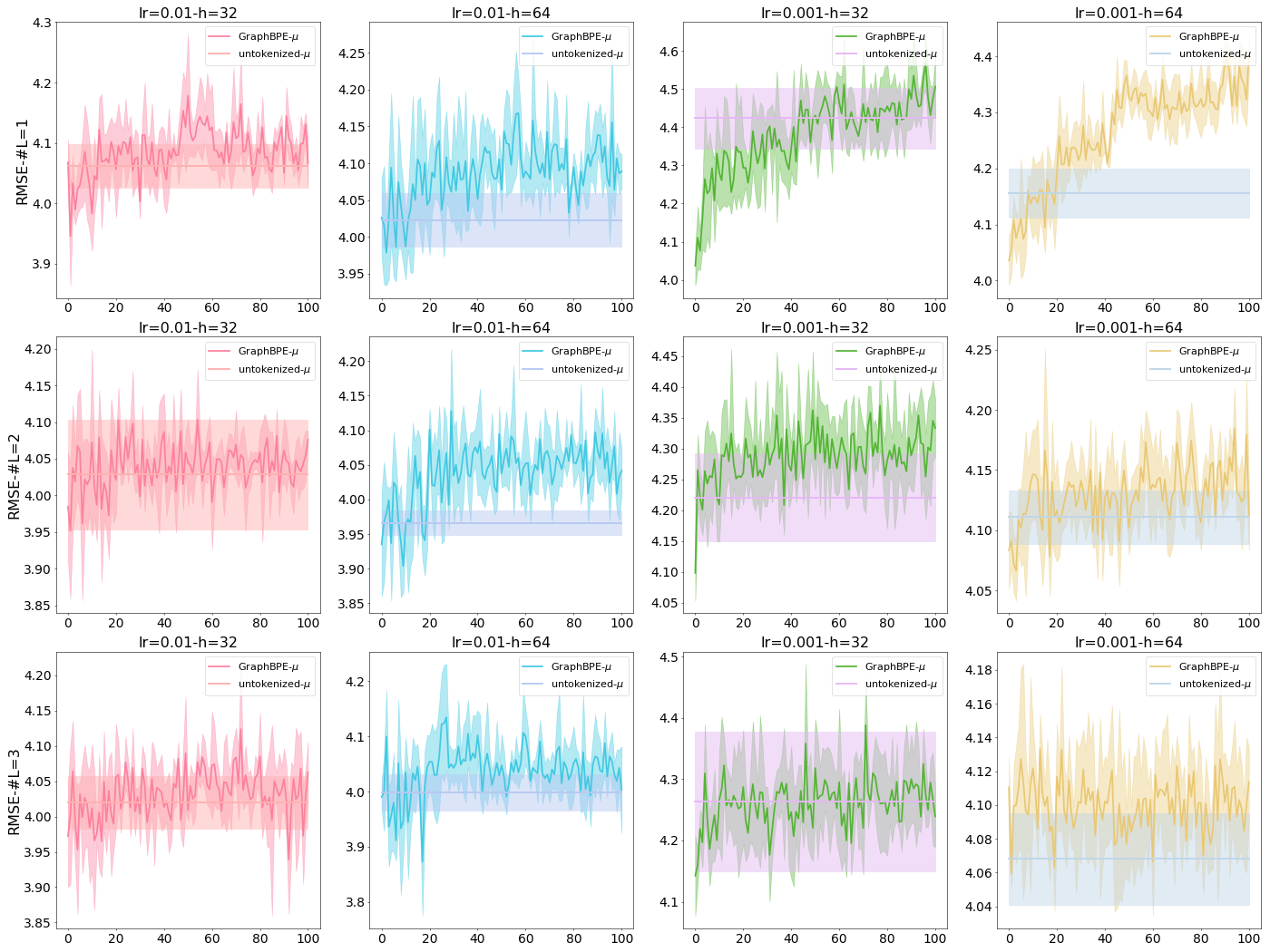
Figure 26: Results of GAT on Freesolv, with RMSE the lower the better

Figure 27: Results of GIN on Freesolv, with RMSE the lower the better

Figure 28: Results of GraphSAGE on Freesolv, with RMSE the lower the better

learning rate		$10^{-2}$		$10^{-3}$
hidden size		$h=32$	$h=64$	$h=32$	$h=64$
$L={1}$	p-value	4:96:1	1:99:1	0:100:1	41:60:0
	metric	71:0:30	66:0:35	36:0:65	101:0:0
$L={2}$	p-value	14:87:0	0:101:0	0:101:0	0:100:1
	metric	84:0:17	38:0:63	71:0:30	31:0:70
$L={3}$	p-value	0:101:0	1:98:2	1:99:1	0:101:0
	metric	26:0:75	26:0:75	53:0:48	77:0:24

Table 44: Centroid on HyperConv

learning rate		$10^{-2}$		$10^{-3}$
hidden size		$h=32$	$h=64$	$h=32$	$h=64$
$L={1}$	p-value	0:93:8	0:101:0	0:92:9	1:100:0
	metric	7:0:94	70:0:31	6:0:95	92:0:9
$L={2}$	p-value	0:88:13	6:95:0	61:40:0	8:93:0
	metric	12:0:89	79:0:22	101:0:0	81:0:20
$L={3}$	p-value	0:99:2	1:100:0	6:95:0	0:101:0
	metric	28:0:73	62:0:39	89:0:12	89:0:12

Table 45: Chem on HyperConv

learning rate		$10^{-2}$		$10^{-3}$
hidden size		$h=32$	$h=64$	$h=32$	$h=64$
$L={1}$	p-value	8:93:0	1:100:0	0:101:0	0:99:2
	metric	89:0:12	55:0:46	94:0:7	38:0:63
$L={2}$	p-value	1:100:0	0:97:4	6:95:0	0:99:2
	metric	43:0:58	18:0:83	99:0:2	9:0:92
$L={3}$	p-value	1:100:0	0:95:6	0:100:1	0:101:0
	metric	60:0:41	17:0:84	50:0:51	61:0:40

Table 46: H2g on HyperConv

learning rate		$10^{-2}$		$10^{-3}$
hidden size		$h=32$	$h=64$	$h=32$	$h=64$
$L={1}$	p-value	0:101:0	0:94:7	0:101:0	0:101:0
	metric	43:0:58	1:0:100	101:0:0	101:0:0
$L={2}$	p-value	1:98:2	1:97:3	0:101:0	1:100:0
	metric	41:0:60	43:0:58	101:0:0	83:0:18
$L={3}$	p-value	0:101:0	0:101:0	0:99:2	2:99:0
	metric	38:0:63	73:0:28	19:0:82	95:0:6

Table 47: Centroid on HGNN++

learning rate		$10^{-2}$		$10^{-3}$
hidden size		$h=32$	$h=64$	$h=32$	$h=64$
$L={1}$	p-value	0:87:14	0:73:28	4:97:0	0:101:0
	metric	6:0:95	1:0:100	96:0:5	56:0:45
$L={2}$	p-value	0:91:10	0:101:0	0:100:1	11:90:0
	metric	7:0:94	43:0:58	42:0:59	81:0:20
$L={3}$	p-value	0:97:4	0:99:2	1:100:0	1:98:2
	metric	5:0:96	42:0:59	59:0:42	22:0:79

Table 48: Chem on HGNN++

learning rate		$10^{-2}$		$10^{-3}$
hidden size		$h=32$	$h=64$	$h=32$	$h=64$
$L={1}$	p-value	10:91:0	1:100:0	0:101:0	0:99:2
	metric	95:0:6	84:0:17	38:0:63	33:0:68
$L={2}$	p-value	0:100:1	0:97:4	0:79:22	0:82:19
	metric	24:0:77	13:0:88	5:0:96	2:0:99
$L={3}$	p-value	0:99:2	13:88:0	0:89:12	0:95:6
	metric	35:0:66	100:0:1	0:0:101	19:0:82

Table 49: H2g on HGNN++

learning rate		$10^{-2}$		$10^{-3}$
hidden size		$h=32$	$h=64$	$h=32$	$h=64$
$L={1}$	p-value	7:94:0	0:99:2	0:97:4	0:101:0
	metric	79:0:22	27:0:74	5:0:96	92:0:9
$L={2}$	p-value	2:99:0	2:99:0	0:101:0	0:95:6
	metric	81:0:20	34:0:67	35:0:66	21:0:80
$L={3}$	p-value	1:100:0	0:92:9	0:39:62	0:65:36
	metric	75:0:26	9:0:92	0:0:101	2:0:99

Table 50: Centroid on HNHN

learning rate		$10^{-2}$		$10^{-3}$
hidden size		$h=32$	$h=64$	$h=32$	$h=64$
$L={1}$	p-value	26:75:0	0:99:2	0:100:1	4:97:0
	metric	98:0:3	39:0:62	19:0:82	99:0:2
$L={2}$	p-value	0:101:0	0:97:4	20:81:0	3:98:0
	metric	71:0:30	30:0:71	97:0:4	91:0:10
$L={3}$	p-value	0:100:1	1:99:1	1:99:1	14:87:0
	metric	71:0:30	41:0:60	38:0:63	99:0:2

Table 51: Chem on HNHN

learning rate		$10^{-2}$		$10^{-3}$
hidden size		$h=32$	$h=64$	$h=32$	$h=64$
$L={1}$	p-value	0:94:7	0:101:0	0:67:34	0:96:5
	metric	24:0:77	38:0:63	0:0:101	8:0:93
$L={2}$	p-value	0:101:0	35:66:0	0:100:1	6:95:0
	metric	49:0:52	99:0:2	26:0:75	76:0:25
$L={3}$	p-value	0:101:0	2:99:0	0:93:8	0:90:11
	metric	83:0:18	69:0:32	12:0:89	3:0:98

Table 52: H2g on HNHN

Table 53: Performance comparison on accuracy with p-value $<0.05$ and metric value on Freesolv. For each triplet $a$:$b$:$c$, $a,b,c$ denote the number of times GraphBPE is statistically/numerically better/the same/worse compared with hypergraphs constructed by Method on Model (e.g., “Centroud on HyperConv” means comparing GraphBPE with Centroid on the HyperConv model).

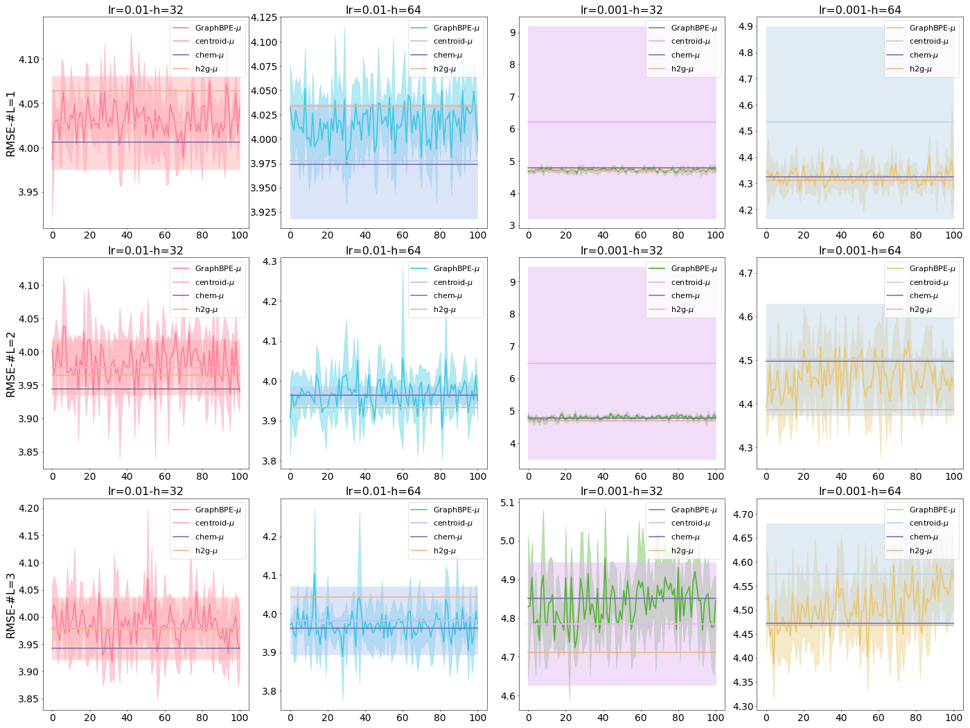
Figure 30: Results of HGNN++ on Freesolv, with RMSE the lower the better

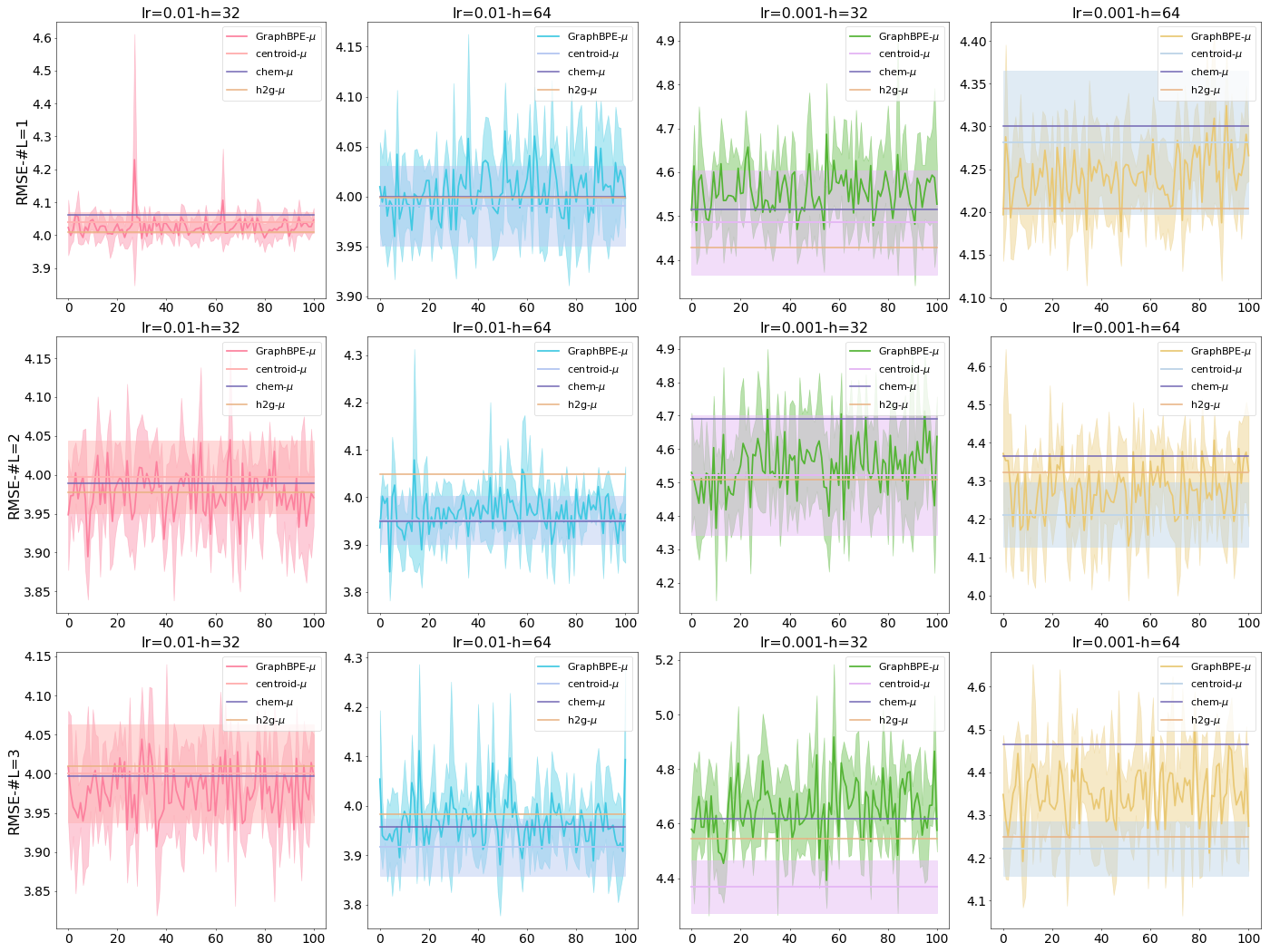
Figure 31: Results of HNHN on Freesolv, with RMSE the lower the better

C.5 Esol

For GNNs, we include the performance comparison results in Table 58, and the visualization over different tokenization steps in Figure 32,  33,  34, and  35 for GCN, GAT, GIN, and GraphSAGE.

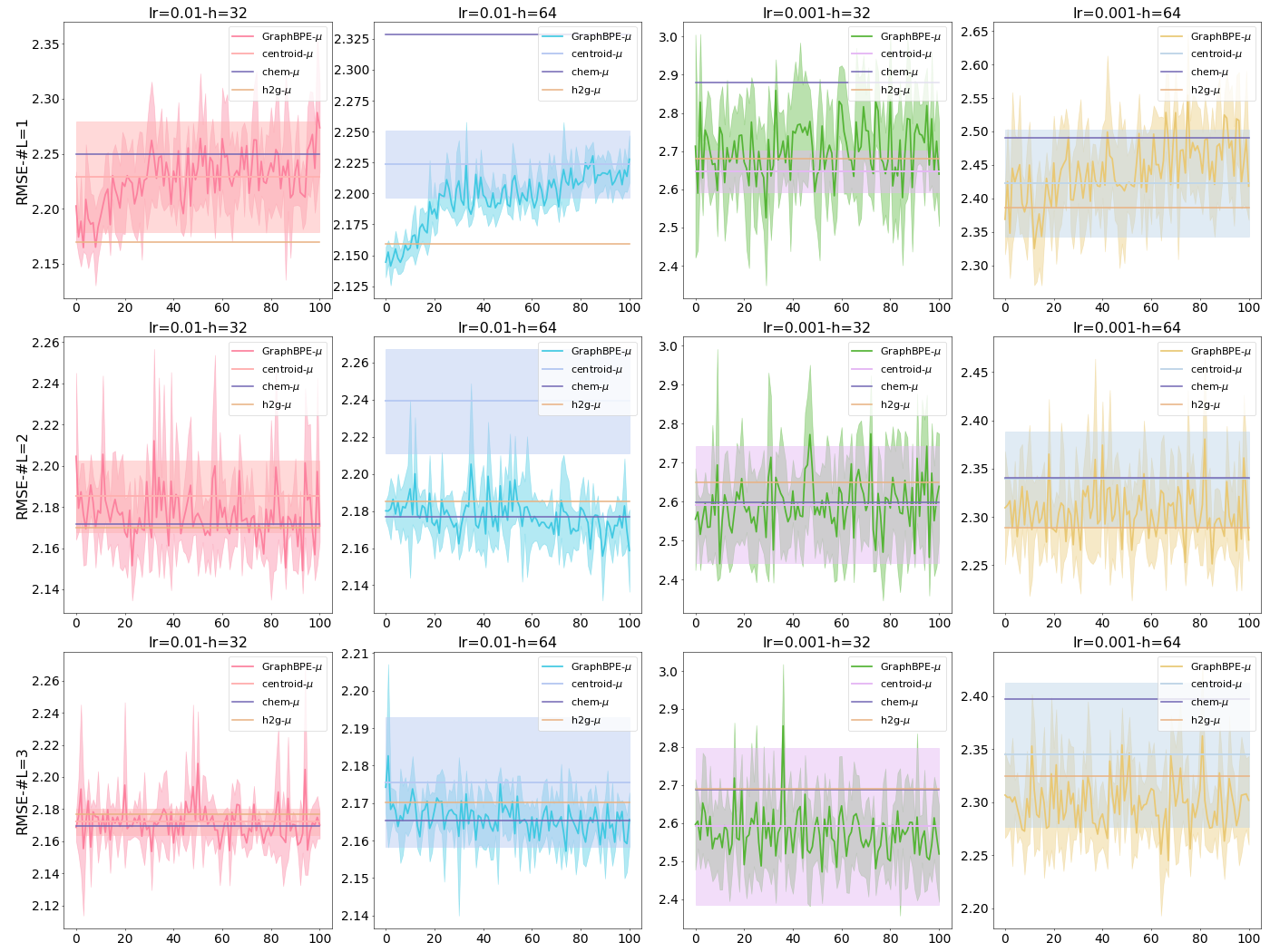
Figure 36: Results of HyperConv on Esol, with RMSE the lower the better

For HyperGNNs, we include the performance comparison results in Table 68, and the visualization over different tokenization steps in Figure 36,  37, and  38 for HyperConv, HGNN++, and HNHN.

learning rate		$10^{-2}$		$10^{-3}$
hidden size		$h=32$	$h=64$	$h=32$	$h=64$
$L={1}$	p-value	0:97:4	12:85:4	0:94:7	0:94:7
	metric	24:0:77	64:0:37	38:0:63	30:0:71
$L={2}$	p-value	0:101:0	0:98:3	0:94:7	0:48:53
	metric	55:0:46	43:0:58	17:0:84	0:0:101
$L={3}$	p-value	1:100:0	0:27:74	3:98:0	0:92:9
	metric	101:0:0	3:0:98	92:0:9	5:0:96

Table 54: Comparison with p-/metric value of GCN

learning rate		$10^{-2}$		$10^{-3}$
hidden size		$h=32$	$h=64$	$h=32$	$h=64$
$L={1}$	p-value	9:92:0	27:74:0	27:74:0	1:95:5
	metric	90:0:11	95:0:6	100:0:1	20:0:81
$L={2}$	p-value	0:100:1	0:101:0	4:95:2	7:94:0
	metric	34:0:67	18:0:83	40:0:61	92:0:9
$L={3}$	p-value	2:99:0	0:88:13	0:92:9	0:81:20
	metric	95:0:6	0:0:101	7:0:94	3:0:98

Table 55: Comparison with p-/metric value of GIN

learning rate		$10^{-2}$		$10^{-3}$
hidden size		$h=32$	$h=64$	$h=32$	$h=64$
$L={1}$	p-value	31:70:0	75:26:0	14:87:0	29:72:0
	metric	93:0:8	97:0:4	93:0:8	92:0:9
$L={2}$	p-value	0:95:6	1:90:10	3:98:0	3:98:0
	metric	18:0:83	55:0:46	67:0:34	65:0:36
$L={3}$	p-value	0:101:0	7:94:0	0:101:0	9:92:0
	metric	61:0:40	83:0:18	57:0:44	68:0:33

Table 56: Comparison with p-/metric value of GAT

learning rate		$10^{-2}$		$10^{-3}$
hidden size		$h=32$	$h=64$	$h=32$	$h=64$
$L={1}$	p-value	24:77:0	43:49:9	0:96:5	0:101:0
	metric	89:0:12	84:0:17	27:0:74	32:0:69
$L={2}$	p-value	3:98:0	15:85:1	0:101:0	0:97:4
	metric	89:0:12	86:0:15	64:0:37	34:0:67
$L={3}$	p-value	9:92:0	27:73:1	0:98:3	0:86:15
	metric	82:0:19	86:0:15	33:0:68	1:0:100

Table 57: Comparison with p-/metric value of GraphSAGE

Table 58: Performance comparison on accuracy with p-value $<0.05$ and metric value on Esol. For each triplet $a$:$b$:$c$, $a,b,c$ denote the number of times GraphBPE is statistically/numerically better/the same/worse compared with (untokenized) simple graph.

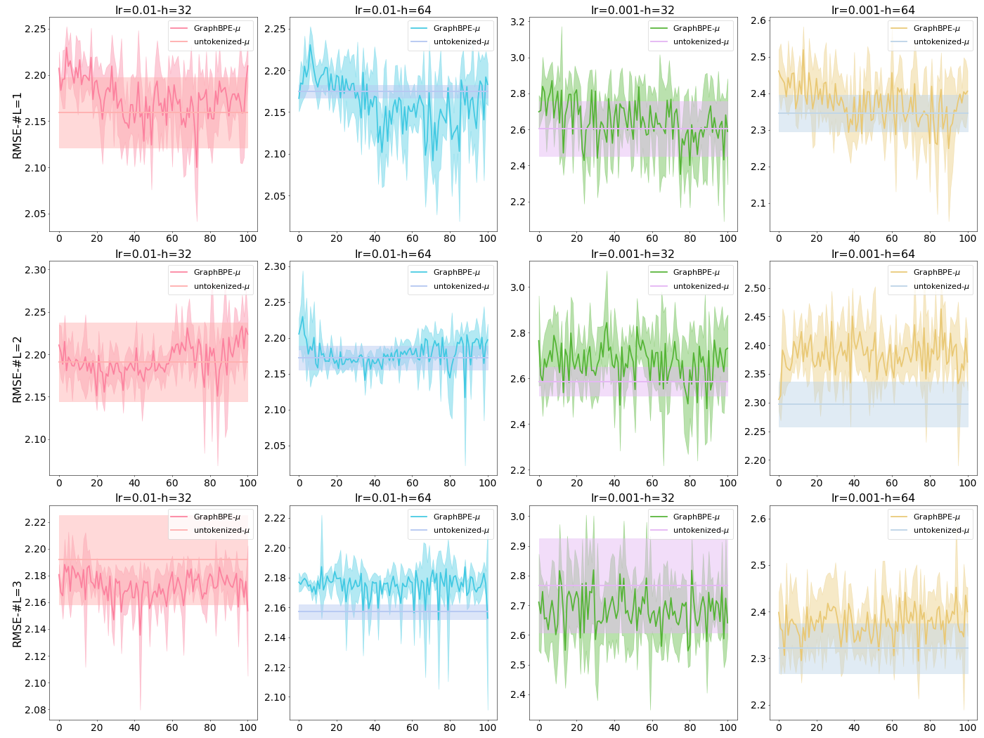
Figure 32: Results of GCN on Esol, with RMSE the lower the better

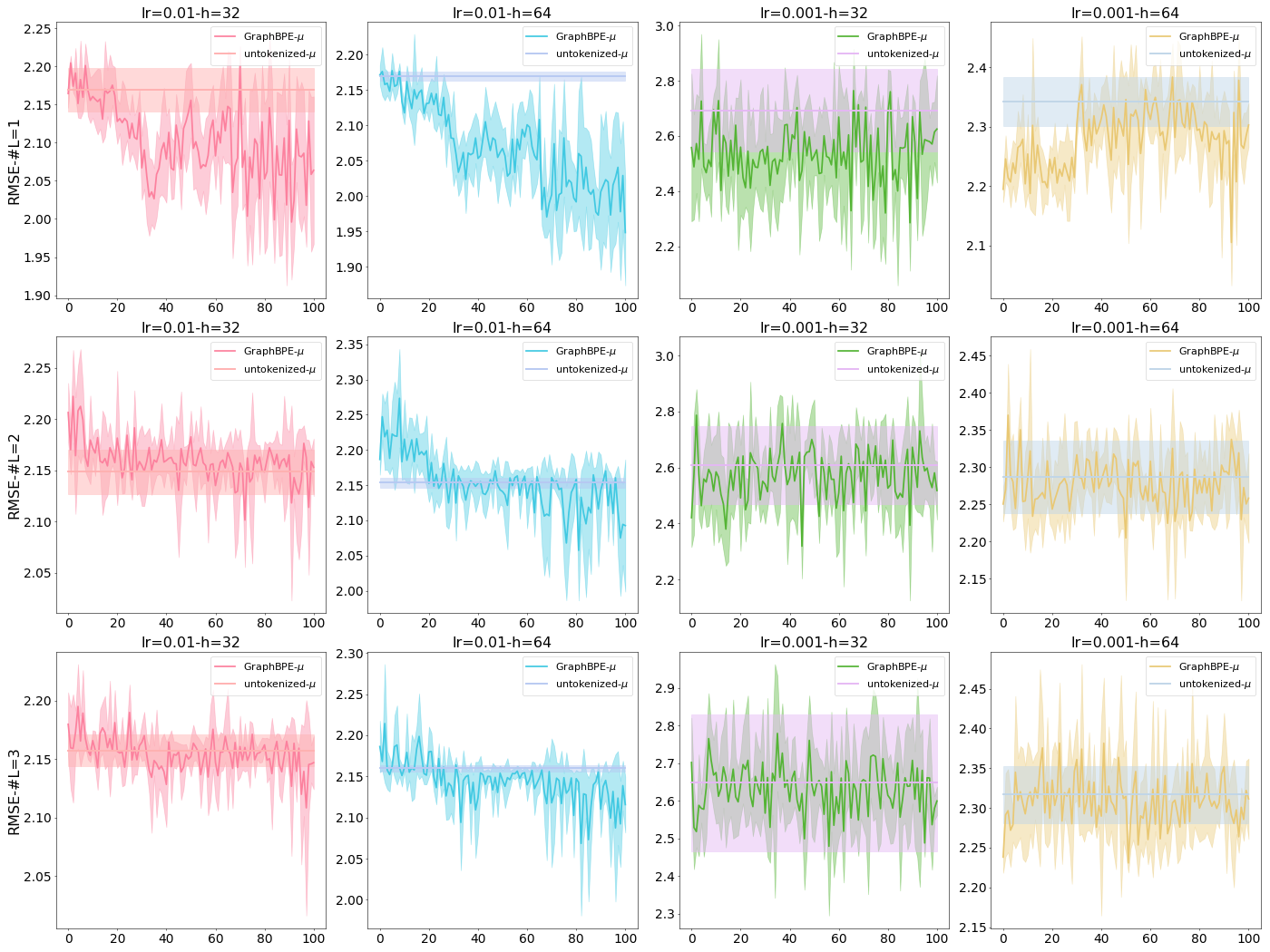
Figure 33: Results of GAT on Esol, with RMSE the lower the better

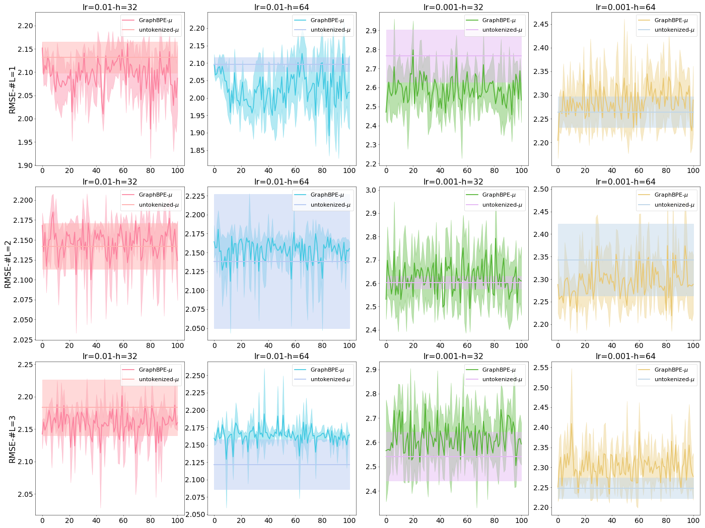
Figure 34: Results of GIN on Esol, with RMSE the lower the better

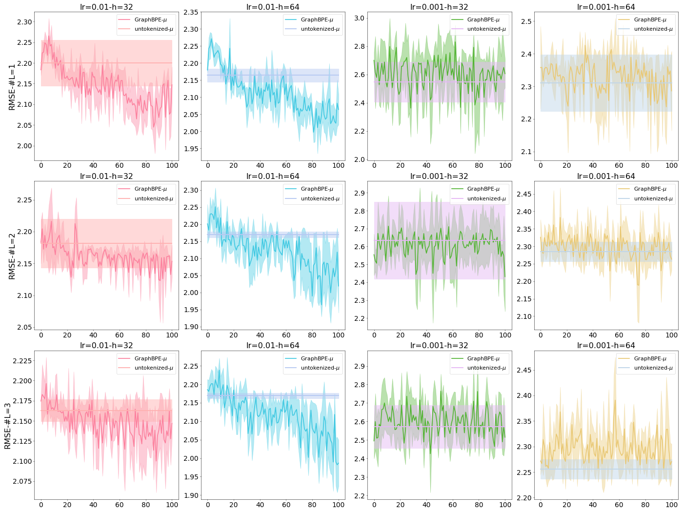
Figure 35: Results of GraphSAGE on Esol, with RMSE the lower the better

learning rate		$10^{-2}$		$10^{-3}$
hidden size		$h=32$	$h=64$	$h=32$	$h=64$
$L={1}$	p-value	1:100:0	17:84:0	0:92:9	0:99:2
	metric	51:0:50	97:0:4	21:0:80	34:0:67
$L={2}$	p-value	6:95:0	87:14:0	0:100:1	4:97:0
	metric	83:0:18	101:0:0	53:0:48	94:0:7
$L={3}$	p-value	2:99:0	0:101:0	0:101:0	4:97:0
	metric	57:0:44	100:0:1	66:0:35	96:0:5

Table 59: Centroid on HyperConv

learning rate		$10^{-2}$		$10^{-3}$
hidden size		$h=32$	$h=64$	$h=32$	$h=64$
$L={1}$	p-value	2:99:0	101:0:0	35:66:0	3:98:0
	metric	85:0:16	101:0:0	101:0:0	90:0:11
$L={2}$	p-value	0:101:0	0:99:2	5:96:0	9:92:0
	metric	36:0:65	51:0:50	57:0:44	94:0:7
$L={3}$	p-value	1:99:1	1:99:1	20:80:1	10:91:0
	metric	43:0:58	45:0:56	98:0:3	101:0:0

Table 60: Chem on HyperConv

learning rate		$10^{-2}$		$10^{-3}$
hidden size		$h=32$	$h=64$	$h=32$	$h=64$
$L={1}$	p-value	0:57:44	1:20:80	0:100:1	0:99:2
	metric	2:0:99	12:0:89	41:0:60	8:0:93
$L={2}$	p-value	2:98:1	8:93:0	0:101:0	0:99:2
	metric	31:0:70	87:0:14	82:0:19	26:0:75
$L={3}$	p-value	11:90:0	9:92:0	7:94:0	3:98:0
	metric	78:0:23	88:0:13	98:0:3	91:0:10

Table 61: H2g on HyperConv

learning rate		$10^{-2}$		$10^{-3}$
hidden size		$h=32$	$h=64$	$h=32$	$h=64$
$L={1}$	p-value	0:98:3	0:101:0	3:98:0	7:94:0
	metric	14:0:87	27:0:74	76:0:25	85:0:16
$L={2}$	p-value	0:101:0	0:101:0	0:81:20	1:97:3
	metric	53:0:48	42:0:59	3:0:98	36:0:65
$L={3}$	p-value	1:99:1	3:96:2	0:100:1	0:90:11
	metric	29:0:72	48:0:53	21:0:80	4:0:97

Table 62: Centroid on HGNN++

learning rate		$10^{-2}$		$10^{-3}$
hidden size		$h=32$	$h=64$	$h=32$	$h=64$
$L={1}$	p-value	2:99:0	0:100:1	29:72:0	38:63:0
	metric	77:0:24	47:0:54	101:0:0	101:0:0
$L={2}$	p-value	0:101:0	1:100:0	12:89:0	43:58:0
	metric	87:0:14	48:0:53	100:0:1	101:0:0
$L={3}$	p-value	3:97:1	1:100:0	32:69:0	17:84:0
	metric	58:0:43	81:0:20	101:0:0	99:0:2

Table 63: Chem on HGNN++

learning rate		$10^{-2}$		$10^{-3}$
hidden size		$h=32$	$h=64$	$h=32$	$h=64$
$L={1}$	p-value	0:101:0	0:101:0	2:99:0	2:95:4
	metric	91:0:10	43:0:58	93:0:8	37:0:64
$L={2}$	p-value	0:101:0	0:101:0	2:97:2	0:101:0
	metric	25:0:76	41:0:60	32:0:69	61:0:40
$L={3}$	p-value	6:94:1	13:88:0	0:101:0	0:98:3
	metric	65:0:36	101:0:0	21:0:80	47:0:54

Table 64: H2g on HGNN++

learning rate		$10^{-2}$		$10^{-3}$
hidden size		$h=32$	$h=64$	$h=32$	$h=64$
$L={1}$	p-value	0:96:5	0:93:8	4:95:2	1:100:0
	metric	24:0:77	11:0:90	74:0:27	48:0:53
$L={2}$	p-value	0:101:0	0:101:0	0:96:5	0:99:2
	metric	58:0:43	37:0:64	19:0:82	36:0:65
$L={3}$	p-value	0:101:0	0:90:11	2:99:0	1:91:9
	metric	58:0:43	5:0:96	64:0:37	13:0:88

Table 65: Centroid on HNHN

learning rate		$10^{-2}$		$10^{-3}$
hidden size		$h=32$	$h=64$	$h=32$	$h=64$
$L={1}$	p-value	0:101:0	0:97:4	2:98:1	11:90:0
	metric	52:0:49	11:0:90	71:0:30	99:0:2
$L={2}$	p-value	0:100:1	0:96:5	0:100:1	0:99:2
	metric	37:0:64	15:0:86	69:0:32	42:0:59
$L={3}$	p-value	0:101:0	5:96:0	1:99:1	0:97:4
	metric	84:0:17	71:0:30	45:0:56	14:0:87

Table 66: Chem on HNHN

learning rate		$10^{-2}$		$10^{-3}$
hidden size		$h=32$	$h=64$	$h=32$	$h=64$
$L={1}$	p-value	1:100:0	0:99:2	0:93:8	0:99:2
	metric	90:0:11	20:0:81	12:0:89	36:0:65
$L={2}$	p-value	1:99:1	0:97:4	7:94:0	1:100:0
	metric	55:0:46	15:0:86	100:0:1	74:0:27
$L={3}$	p-value	0:101:0	0:88:13	0:100:1	10:91:0
	metric	65:0:36	8:0:93	31:0:70	87:0:14

Table 67: H2g on HNHN

Table 68: Performance comparison on accuracy with p-value $<0.05$ and metric value on Esol. For each triplet $a$:$b$:$c$, $a,b,c$ denote the number of times GraphBPE is statistically/numerically better/the same/worse compared with hypergraphs constructed by Method on Model (e.g., “Centroud on HyperConv” means comparing GraphBPE with Centroid on the HyperConv model).

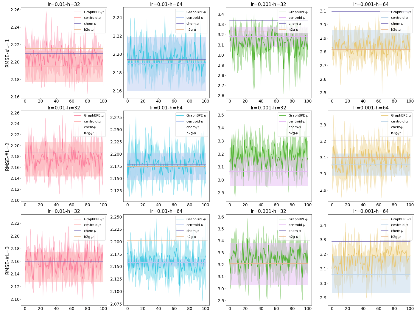
Figure 37: Results of HGNN++ on Esol, with RMSE the lower the better

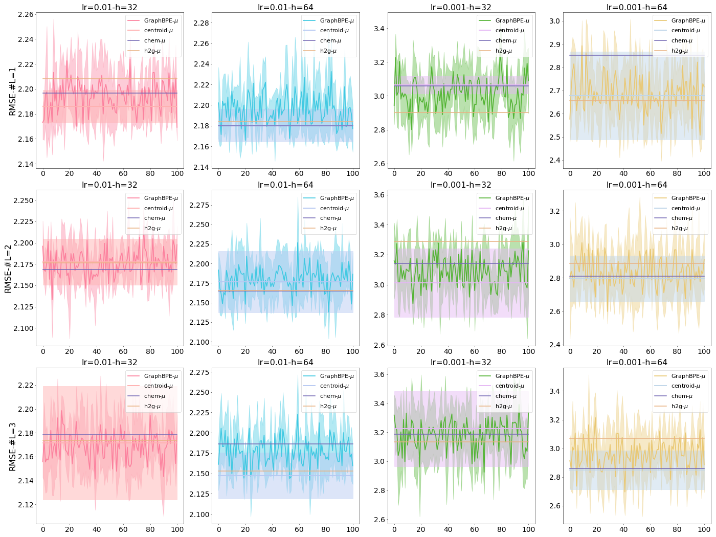
Figure 38: Results of HNHN on Esol, with RMSE the lower the better

C.6 Lipophilicity

For GNNs, we include the performance comparison results in Table 73, and the visualization over different tokenization steps in Figure 39,  40,  41, and  42 for GCN, GAT, GIN, and GraphSAGE.

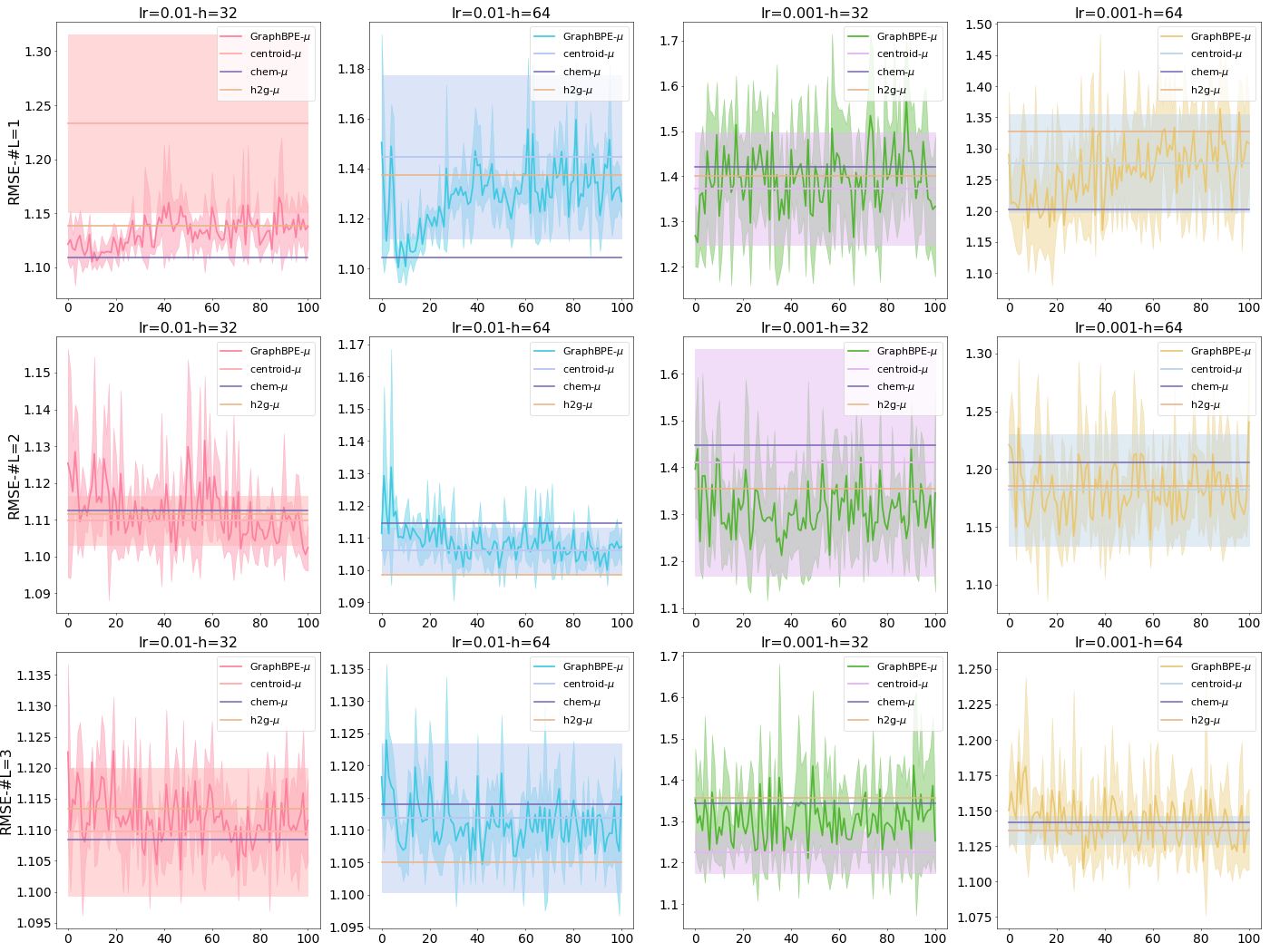
Figure 43: Results of HyperConv on Lipophilicity, with RMSE the lower the better

For HyperGNNs, we include the performance comparison results in Table 83, and the visualization over different tokenization steps in Figure 43,  44, and  45 for HyperConv, HGNN++, and HNHN.

learning rate		$10^{-2}$		$10^{-3}$
hidden size		$h=32$	$h=64$	$h=32$	$h=64$
$L={1}$	p-value	0:0:101	0:0:101	0:83:18	0:37:64
	metric	0:0:101	0:0:101	6:0:95	0:0:101
$L={2}$	p-value	0:101:0	0:94:7	0:101:0	0:100:1
	metric	51:0:50	11:0:90	62:0:39	39:0:62
$L={3}$	p-value	5:96:0	50:51:0	0:97:4	0:93:8
	metric	72:0:29	95:0:6	16:0:85	13:0:88

Table 69: Comparison with p-/metric value of GCN

learning rate		$10^{-2}$		$10^{-3}$
hidden size		$h=32$	$h=64$	$h=32$	$h=64$
$L={1}$	p-value	0:98:3	0:93:8	0:88:13	5:95:1
	metric	4:0:97	10:0:91	4:0:97	57:0:44
$L={2}$	p-value	0:99:2	2:99:0	34:67:0	0:100:1
	metric	19:0:82	47:0:54	100:0:1	40:0:61
$L={3}$	p-value	6:95:0	0:100:1	15:86:0	1:100:0
	metric	52:0:49	18:0:83	98:0:3	86:0:15

Table 70: Comparison with p-/metric value of GIN

learning rate		$10^{-2}$		$10^{-3}$
hidden size		$h=32$	$h=64$	$h=32$	$h=64$
$L={1}$	p-value	0:95:6	0:62:39	4:97:0	0:101:0
	metric	25:0:76	1:0:100	66:0:35	72:0:29
$L={2}$	p-value	0:98:3	0:97:4	0:91:10	0:97:4
	metric	19:0:82	27:0:74	6:0:95	5:0:96
$L={3}$	p-value	0:91:10	5:94:2	0:99:2	8:93:0
	metric	5:0:96	47:0:54	21:0:80	61:0:40

Table 71: Comparison with p-/metric value of GAT

learning rate		$10^{-2}$		$10^{-3}$
hidden size		$h=32$	$h=64$	$h=32$	$h=64$
$L={1}$	p-value	0:68:33	0:84:17	23:78:0	0:101:0
	metric	0:0:101	4:0:97	100:0:1	101:0:0
$L={2}$	p-value	0:86:15	0:26:75	0:72:29	0:30:71
	metric	5:0:96	0:0:101	0:0:101	0:0:101
$L={3}$	p-value	0:96:5	0:92:9	2:98:1	0:85:16
	metric	18:0:83	15:0:86	40:0:61	1:0:100

Table 72: Comparison with p-/metric value of GraphSAGE

Table 73: Performance comparison on accuracy with p-value $<0.05$ and metric value on Lipophilicity. For each triplet $a$:$b$:$c$, $a,b,c$ denote the number of times GraphBPE is statistically/numerically better/the same/worse compared with (untokenized) simple graph.

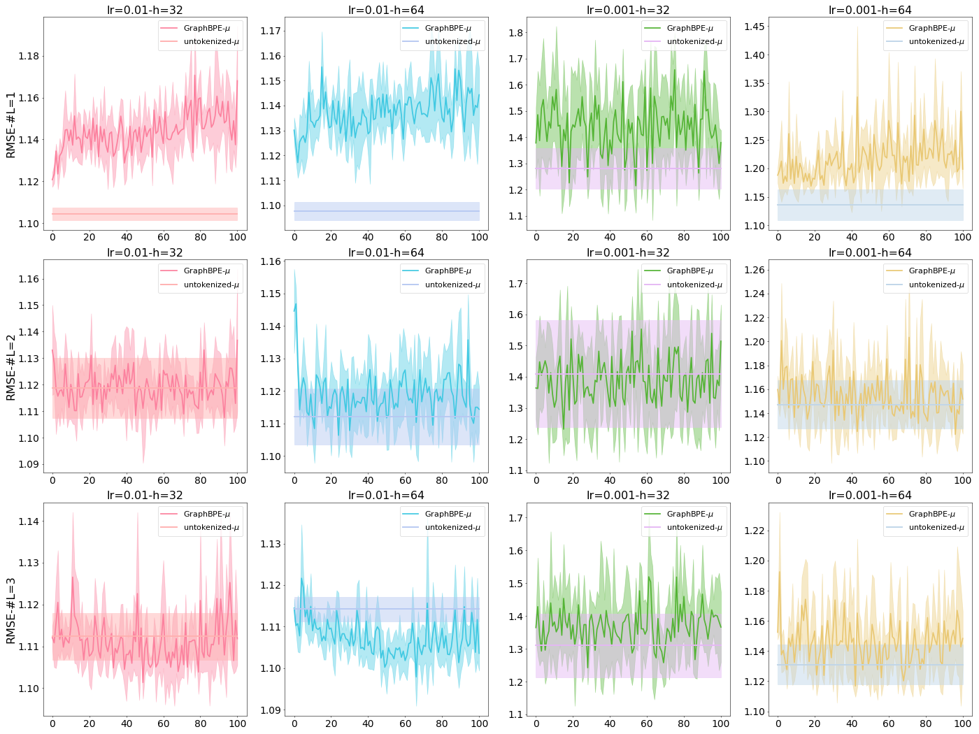
Figure 39: Results of GCN on Lipophilicity, with RMSE the lower the better

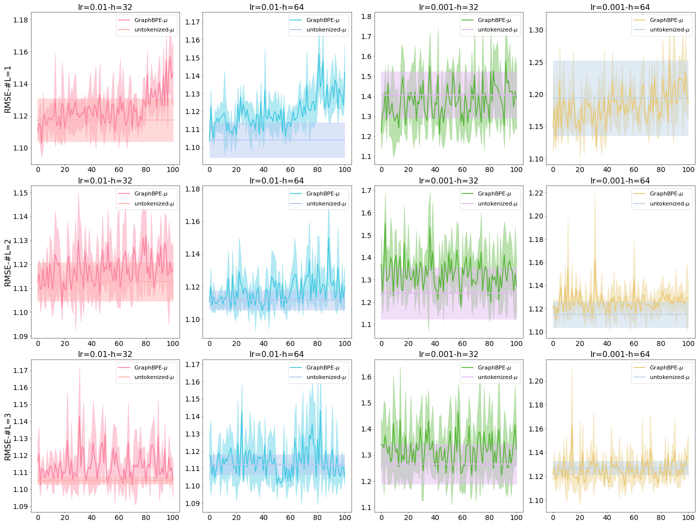
Figure 40: Results of GAT on Lipophilicity, with RMSE the lower the better

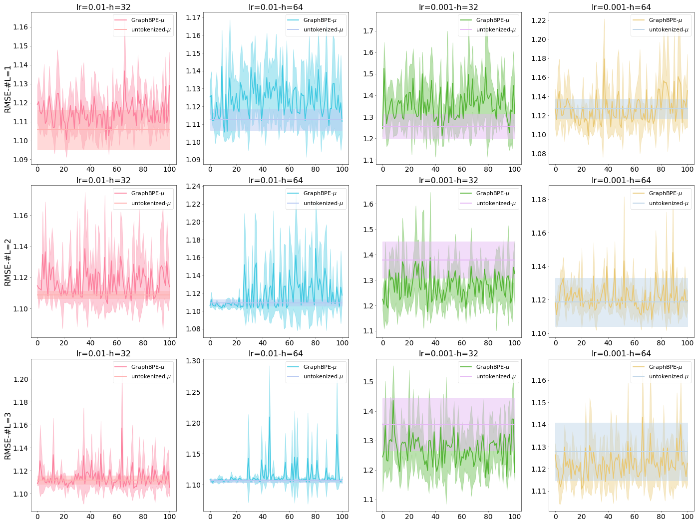
Figure 41: Results of GIN on Lipophilicity, with RMSE the lower the better

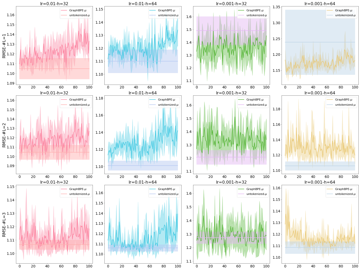
Figure 42: Results of GraphSAGE on Lipophilicity, with RMSE the lower the better

learning rate		$10^{-2}$		$10^{-3}$
hidden size		$h=32$	$h=64$	$h=32$	$h=64$
$L={1}$	p-value	22:79:0	2:99:0	0:99:2	2:99:0
	metric	101:0:0	91:0:10	34:0:67	61:0:40
$L={2}$	p-value	1:97:3	0:98:3	0:101:0	0:100:1
	metric	41:0:60	25:0:76	95:0:6	56:0:45
$L={3}$	p-value	0:101:0	0:101:0	0:90:11	4:93:4
	metric	27:0:74	67:0:34	2:0:99	35:0:66

Table 74: Centroid on HyperConv

learning rate		$10^{-2}$		$10^{-3}$
hidden size		$h=32$	$h=64$	$h=32$	$h=64$
$L={1}$	p-value	0:75:26	0:27:74	0:101:0	0:93:8
	metric	2:0:99	2:0:99	67:0:34	10:0:91
$L={2}$	p-value	1:100:0	9:92:0	8:93:0	11:90:0
	metric	60:0:41	91:0:10	101:0:0	86:0:15
$L={3}$	p-value	1:88:12	7:94:0	2:99:0	0:101:0
	metric	17:0:84	84:0:17	81:0:20	52:0:49

Table 75: Chem on HyperConv

learning rate		$10^{-2}$		$10^{-3}$
hidden size		$h=32$	$h=64$	$h=32$	$h=64$
$L={1}$	p-value	0:101:0	13:88:0	2:98:1	0:101:0
	metric	67:0:34	81:0:20	57:0:44	93:0:8
$L={2}$	p-value	0:100:1	0:45:56	1:100:0	1:99:1
	metric	52:0:49	0:0:101	84:0:17	62:0:39
$L={3}$	p-value	1:100:0	0:94:7	0:101:0	1:97:3
	metric	70:0:31	2:0:99	91:0:10	35:0:66

Table 76: H2g on HyperConv

learning rate		$10^{-2}$		$10^{-3}$
hidden size		$h=32$	$h=64$	$h=32$	$h=64$
$L={1}$	p-value	0:94:7	0:100:1	1:100:0	0:99:2
	metric	24:0:77	22:0:79	67:0:34	24:0:77
$L={2}$	p-value	4:97:0	1:94:6	1:98:2	0:101:0
	metric	79:0:22	38:0:63	30:0:71	56:0:45
$L={3}$	p-value	0:99:2	0:99:2	1:99:1	2:99:0
	metric	23:0:78	8:0:93	73:0:28	97:0:4

Table 77: Centroid on HGNN++

learning rate		$10^{-2}$		$10^{-3}$
hidden size		$h=32$	$h=64$	$h=32$	$h=64$
$L={1}$	p-value	8:93:0	2:98:1	48:53:0	62:39:0
	metric	90:0:11	50:0:51	101:0:0	101:0:0
$L={2}$	p-value	0:101:0	8:93:0	8:93:0	8:93:0
	metric	71:0:30	71:0:30	92:0:9	95:0:6
$L={3}$	p-value	0:99:2	19:82:0	17:84:0	5:96:0
	metric	26:0:75	99:0:2	93:0:8	80:0:21

Table 78: Chem on HGNN++

learning rate		$10^{-2}$		$10^{-3}$
hidden size		$h=32$	$h=64$	$h=32$	$h=64$
$L={1}$	p-value	0:100:1	0:101:0	0:98:3	2:99:0
	metric	28:0:73	51:0:50	40:0:61	96:0:5
$L={2}$	p-value	0:93:8	32:69:0	1:97:3	0:96:5
	metric	2:0:99	99:0:2	32:0:69	15:0:86
$L={3}$	p-value	0:88:13	2:99:0	0:98:3	1:98:2
	metric	10:0:91	59:0:42	12:0:89	45:0:56

Table 79: H2g on HGNN++

learning rate		$10^{-2}$		$10^{-3}$
hidden size		$h=32$	$h=64$	$h=32$	$h=64$
$L={1}$	p-value	0:96:5	11:90:0	0:96:5	0:101:0
	metric	9:0:92	98:0:3	29:0:72	78:0:23
$L={2}$	p-value	0:99:2	2:99:0	3:98:0	0:89:12
	metric	16:0:85	66:0:35	101:0:0	6:0:95
$L={3}$	p-value	0:99:2	0:87:14	2:98:1	0:97:4
	metric	34:0:67	7:0:94	61:0:40	10:0:91

Table 80: Centroid on HNHN

learning rate		$10^{-2}$		$10^{-3}$
hidden size		$h=32$	$h=64$	$h=32$	$h=64$
$L={1}$	p-value	2:97:2	2:99:0	10:91:0	0:101:0
	metric	56:0:45	64:0:37	99:0:2	90:0:11
$L={2}$	p-value	0:101:0	0:98:3	2:98:1	6:95:0
	metric	86:0:15	39:0:62	46:0:55	88:0:13
$L={3}$	p-value	0:99:2	0:98:3	0:98:3	0:101:0
	metric	34:0:67	42:0:59	9:0:92	43:0:58

Table 81: Chem on HNHN

learning rate		$10^{-2}$		$10^{-3}$
hidden size		$h=32$	$h=64$	$h=32$	$h=64$
$L={1}$	p-value	0:90:11	0:97:4	1:100:0	0:101:0
	metric	3:0:98	15:0:86	91:0:10	29:0:72
$L={2}$	p-value	2:99:0	0:95:6	9:91:1	0:100:1
	metric	85:0:16	21:0:80	90:0:11	48:0:53
$L={3}$	p-value	13:88:0	0:101:0	1:100:0	0:88:13
	metric	93:0:8	48:0:53	87:0:14	2:0:99

Table 82: H2g on HNHN

Table 83: Performance comparison on accuracy with p-value $<0.05$ and metric value on Lipophilicity. For each triplet $a$:$b$:$c$, $a,b,c$ denote the number of times GraphBPE is statistically/numerically better/the same/worse compared with hypergraphs constructed by Method on Model (e.g., “Centroud on HyperConv” means comparing GraphBPE with Centroid on the HyperConv model).

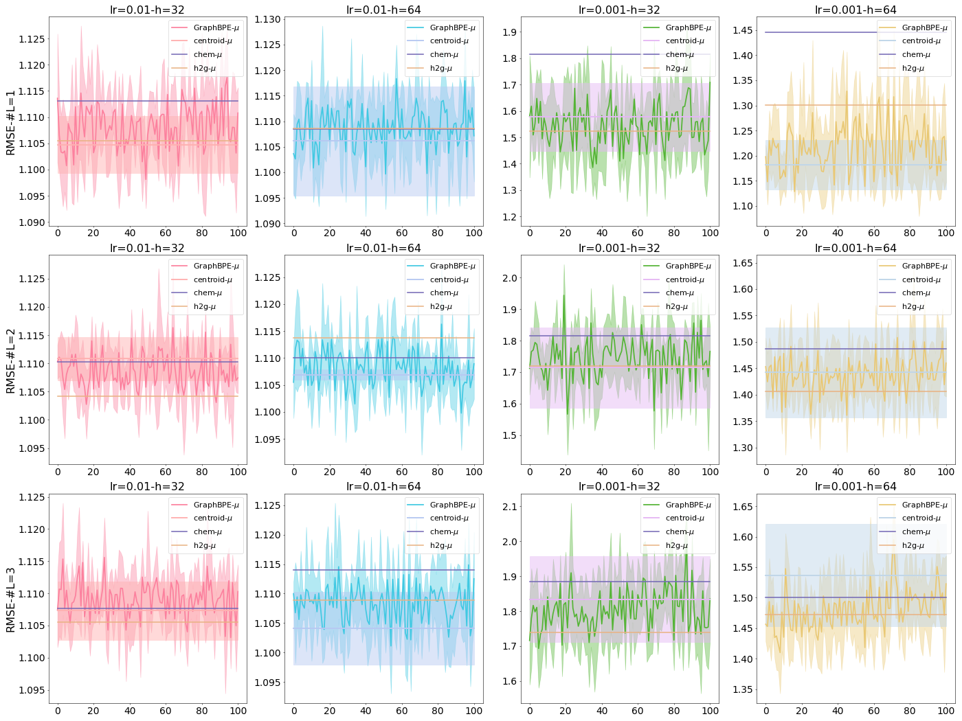
Figure 44: Results of HGNN++ on Lipophilicity, with RMSE the lower the better

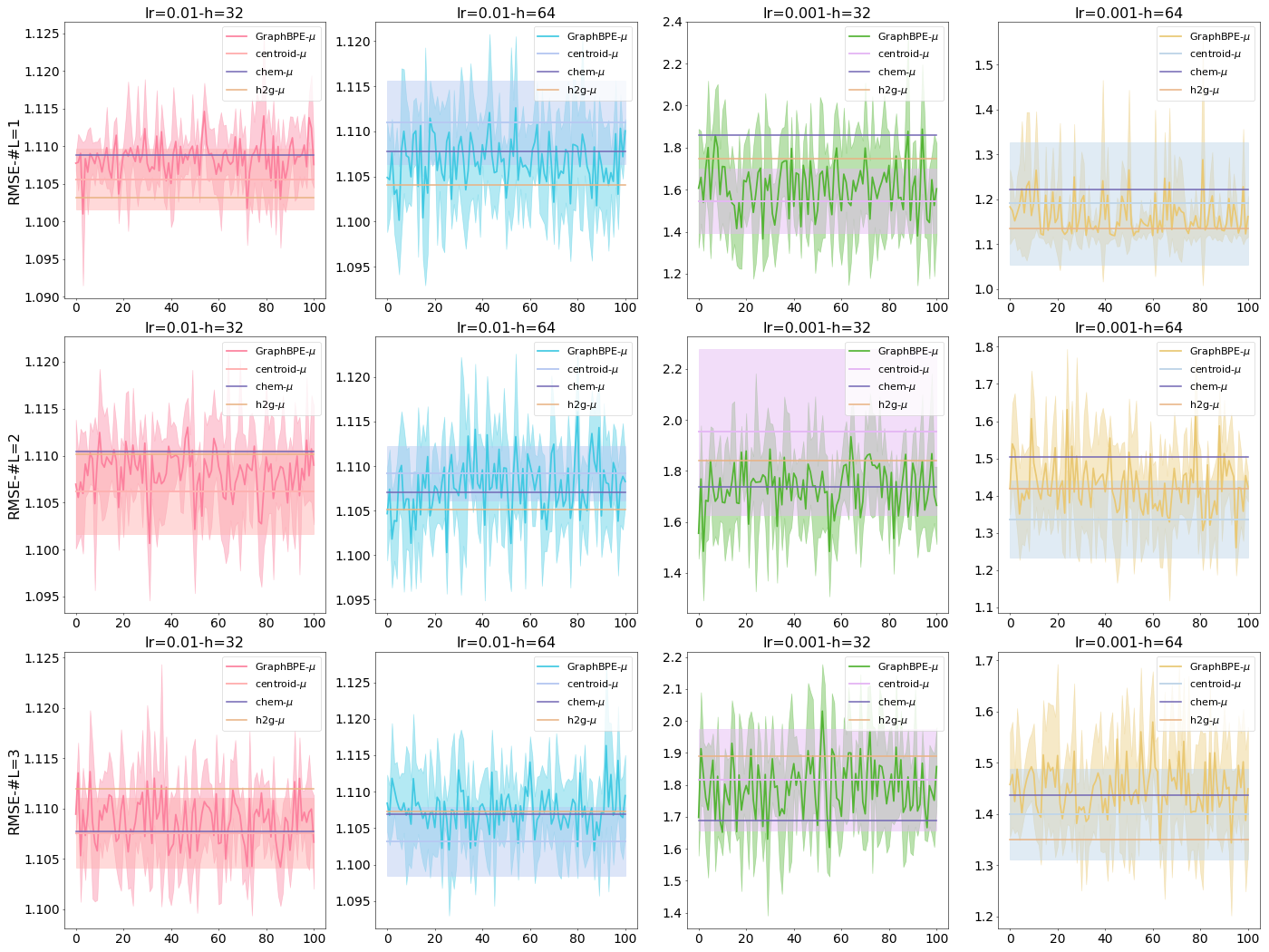
Figure 45: Results of HNHN on Lipophilicity, with RMSE the lower the better

References

- Almazrouei et al. (2023) Almazrouei, E., Alobeidli, H., Alshamsi, A., Cappelli, A., Cojocaru, R., Debbah, M., Étienne Goffinet, Hesslow, D., Launay, J., Malartic, Q., Mazzotta, D., Noune, B., Pannier, B., and Penedo, G. The falcon series of open language models, 2023.
- Bai et al. (2020) Bai, S., Zhang, F., and Torr, P. H. S. Hypergraph convolution and hypergraph attention, 2020.
- Brown et al. (2020) Brown, T. B., Mann, B., Ryder, N., Subbiah, M., Kaplan, J., Dhariwal, P., Neelakantan, A., Shyam, P., Sastry, G., Askell, A., Agarwal, S., Herbert-Voss, A., Krueger, G., Henighan, T., Child, R., Ramesh, A., Ziegler, D. M., Wu, J., Winter, C., Hesse, C., Chen, M., Sigler, E., Litwin, M., Gray, S., Chess, B., Clark, J., Berner, C., McCandlish, S., Radford, A., Sutskever, I., and Amodei, D. Language models are few-shot learners, 2020.
- Dehaspe et al. (1998) Dehaspe, L., Toivonen, H., and King, R. D. Finding frequent substructures in chemical compounds. In Proceedings of the Fourth International Conference on Knowledge Discovery and Data Mining, KDD’98, pp. 30–36. AAAI Press, 1998.
- Dong et al. (2020) Dong, Y., Sawin, W., and Bengio, Y. Hnhn: Hypergraph networks with hyperedge neurons, 2020.
- Feng et al. (2019) Feng, Y., You, H., Zhang, Z., Ji, R., and Gao, Y. Hypergraph neural networks, 2019.
- Gage (1994) Gage, P. A new algorithm for data compression. The C Users Journal archive, 12:23–38, 1994. URL https://api.semanticscholar.org/CorpusID:59804030.
- Gao et al. (2023) Gao, Y., Feng, Y., Ji, S., and Ji, R. Hgnn+: General hypergraph neural networks. IEEE Transactions on Pattern Analysis and Machine Intelligence, 45(3):3181–3199, 2023. doi: 10.1109/TPAMI.2022.3182052.
- Geng et al. (2023) Geng, Z., Xie, S., Xia, Y., Wu, L., Qin, T., Wang, J., Zhang, Y., Wu, F., and Liu, T.-Y. De novo molecular generation via connection-aware motif mining, 2023.
- Guo et al. (2022) Guo, M., Thost, V., Li, B., Das, P., Chen, J., and Matusik, W. Data-efficient graph grammar learning for molecular generation, 2022.
- Hamilton et al. (2018) Hamilton, W. L., Ying, R., and Leskovec, J. Inductive representation learning on large graphs, 2018.
- He & Singh (2007) He, H. and Singh, A. K. Efficient algorithms for mining significant substructures in graphs with quality guarantees. In Proceedings of the 7th IEEE International Conference on Data Mining (ICDM 2007), October 28-31, 2007, Omaha, Nebraska, USA, pp. 163–172. IEEE Computer Society, 2007. doi: 10.1109/ICDM.2007.11. URL https://doi.org/10.1109/ICDM.2007.11.
- Ioffe & Szegedy (2015) Ioffe, S. and Szegedy, C. Batch normalization: Accelerating deep network training by reducing internal covariate shift, 2015.
- Jin et al. (2020) Jin, W., Barzilay, R., and Jaakkola, T. Hierarchical generation of molecular graphs using structural motifs, 2020.
- Kipf & Welling (2017) Kipf, T. N. and Welling, M. Semi-supervised classification with graph convolutional networks, 2017.
- Kong et al. (2022) Kong, X., Huang, W., Tan, Z., and Liu, Y. Molecule generation by principal subgraph mining and assembling. In Oh, A. H., Agarwal, A., Belgrave, D., and Cho, K. (eds.), Advances in Neural Information Processing Systems, 2022. URL https://openreview.net/forum?id=ATfARCRmM-a.
- Kudo (2018) Kudo, T. Subword regularization: Improving neural network translation models with multiple subword candidates. In Gurevych, I. and Miyao, Y. (eds.), Proceedings of the 56th Annual Meeting of the Association for Computational Linguistics (Volume 1: Long Papers), pp. 66–75, Melbourne, Australia, July 2018. Association for Computational Linguistics. doi: 10.18653/v1/P18-1007. URL https://aclanthology.org/P18-1007.
- Kudo & Richardson (2018) Kudo, T. and Richardson, J. SentencePiece: A simple and language independent subword tokenizer and detokenizer for neural text processing. In Blanco, E. and Lu, W. (eds.), Proceedings of the 2018 Conference on Empirical Methods in Natural Language Processing: System Demonstrations, pp. 66–71, Brussels, Belgium, November 2018. Association for Computational Linguistics. doi: 10.18653/v1/D18-2012. URL https://aclanthology.org/D18-2012.
- Kuramochi & Karypis (2001) Kuramochi, M. and Karypis, G. Frequent subgraph discovery. In Proceedings 2001 IEEE International Conference on Data Mining, pp. 313–320, 2001. doi: 10.1109/ICDM.2001.989534.
- Landrum et al. (2006) Landrum, G. et al. Rdkit: Open-source cheminformatics, 2006.
- Lee et al. (2024) Lee, S., Lee, S., Kawaguchi, K., and Hwang, S. J. Drug discovery with dynamic goal-aware fragments, 2024.
- Li et al. (2023) Li, B., Lin, M., Chen, T., and Wang, L. FG-BERT: a generalized and self-supervised functional group-based molecular representation learning framework for properties prediction. Briefings in Bioinformatics, 24(6):bbad398, 11 2023. ISSN 1477-4054. doi: 10.1093/bib/bbad398. URL https://doi.org/10.1093/bib/bbad398.
- Liu et al. (2024) Liu, Z., Shi, Y., Zhang, A., Zhang, E., Kawaguchi, K., Wang, X., and Chua, T.-S. Rethinking tokenizer and decoder in masked graph modeling for molecules, 2024.
- Luong & Singh (2023) Luong, K.-D. and Singh, A. Fragment-based pretraining and finetuning on molecular graphs, 2023.
- Morris et al. (2020) Morris, C., Kriege, N. M., Bause, F., Kersting, K., Mutzel, P., and Neumann, M. Tudataset: A collection of benchmark datasets for learning with graphs, 2020.
- Ranu & Singh (2009) Ranu, S. and Singh, A. K. Graphsig: A scalable approach to mining significant subgraphs in large graph databases. 2009 IEEE 25th International Conference on Data Engineering, pp. 844–855, 2009. URL https://api.semanticscholar.org/CorpusID:16853287.
- Schuster & Nakajima (2012) Schuster, M. and Nakajima, K. Japanese and korean voice search. 2012 IEEE International Conference on Acoustics, Speech and Signal Processing (ICASSP), pp. 5149–5152, 2012. URL https://api.semanticscholar.org/CorpusID:22320655.
- Sennrich et al. (2016) Sennrich, R., Haddow, B., and Birch, A. Neural machine translation of rare words with subword units, 2016.
- Touvron et al. (2023a) Touvron, H., Lavril, T., Izacard, G., Martinet, X., Lachaux, M.-A., Lacroix, T., Rozière, B., Goyal, N., Hambro, E., Azhar, F., Rodriguez, A., Joulin, A., Grave, E., and Lample, G. Llama: Open and efficient foundation language models, 2023a.
- Touvron et al. (2023b) Touvron, H., Martin, L., Stone, K., Albert, P., Almahairi, A., Babaei, Y., Bashlykov, N., Batra, S., Bhargava, P., Bhosale, S., Bikel, D., Blecher, L., Ferrer, C. C., Chen, M., Cucurull, G., Esiobu, D., Fernandes, J., Fu, J., Fu, W., Fuller, B., Gao, C., Goswami, V., Goyal, N., Hartshorn, A., Hosseini, S., Hou, R., Inan, H., Kardas, M., Kerkez, V., Khabsa, M., Kloumann, I., Korenev, A., Koura, P. S., Lachaux, M.-A., Lavril, T., Lee, J., Liskovich, D., Lu, Y., Mao, Y., Martinet, X., Mihaylov, T., Mishra, P., Molybog, I., Nie, Y., Poulton, A., Reizenstein, J., Rungta, R., Saladi, K., Schelten, A., Silva, R., Smith, E. M., Subramanian, R., Tan, X. E., Tang, B., Taylor, R., Williams, A., Kuan, J. X., Xu, P., Yan, Z., Zarov, I., Zhang, Y., Fan, A., Kambadur, M., Narang, S., Rodriguez, A., Stojnic, R., Edunov, S., and Scialom, T. Llama 2: Open foundation and fine-tuned chat models, 2023b.
- Veličković et al. (2018) Veličković, P., Cucurull, G., Casanova, A., Romero, A., Liò, P., and Bengio, Y. Graph attention networks, 2018.
- Wu et al. (2018) Wu, Z., Ramsundar, B., Feinberg, E. N., Gomes, J., Geniesse, C., Pappu, A. S., Leswing, K., and Pande, V. Moleculenet: A benchmark for molecular machine learning, 2018.
- Xu et al. (2019) Xu, K., Hu, W., Leskovec, J., and Jegelka, S. How powerful are graph neural networks?, 2019.
- Yu & Gao (2022) Yu, Z. and Gao, H. Molecular representation learning via heterogeneous motif graph neural networks, 2022.