Designing a Universal Quantum Switch for Arbitrary Quantum Dynamics
Abstract
A quantum switch is a superoperator that, in general, creates a superposition of various causal orders of two or more quantum dynamics that are all divisible in the complete positivity (CP) sense. We introduce a process that we term as the universal quantum switch (UQS), which unlike conventional quantum switches, allows for the construction of a quantum switch that can superpose different causal orders of any set of quantum dynamics, regardless of their CP-divisibility. Our approach also enables the construction of a quantum switch while considering a single environment connected with the system, in contrast to the traditional one. Moreover, we show the UQS provides more advantages in performance for a certain state discrimination task compared to traditional quantum switches. The next question that we address is the following: What is the CP-divisibility characteristic of a dynamics built by acting a quantum switch on CP-divisible or -indivisible dynamics? In this regard, an example is presented where the dynamics created by the action of the UQS on two CP-indivisible dynamics is CP-indivisible. Additionally, we prove a necessary and sufficient condition for the channel created by acting the traditional quantum switch on two CP-divisible dynamics to be CP-divisible. Furthermore, we present some examples of CP-divisible dynamics on which, when the usual quantum switch is operated, the resulting dynamics not only becomes CP-indivisible but also turns into P-indivisible. Our findings demonstrate that quantum switches can build CP-divisible, CP-indivisible, and even P-indivisible dynamics from CP-divisible dynamics, underscoring the versatility of this technique.
I Introduction
Quantum evolutions of isolated systems can be described using unitary maps. However, when a system interacts with an external entity, commonly referred to as the environment, the evolution of the system over time cannot be expressed solely through a unitary transformation. In such scenarios, the system is considered to be open to the environment Rivas and Huelga (2012); Rivas et al. (2014); Breuer et al. (2016); de Vega and Alonso (2017). If the system and the environment are initially in a product state, the evolution of the system from its initial state to any subsequent state can be elucidated using a linear completely positive trace-preserving map (CPTP). Interestingly, the converse is also true, i.e., any CPTP evolution of a system can always be explained by considering the presence of an environment and the composite dynamics of the system-environment set-up to be unitary.
CPTP dynamics of systems can mainly be classified in two ways: (i) CP-divisible and CP-indivisible, and (ii) P-divisible and P-indivisible. CP- and P-indivisibility find extensive applications in a large variety of domains, ranging from quantum information theory Vasile et al. (2011); Chen et al. (2016); Gupta et al. (2022); Roy et al. (2023); Muhuri et al. (2024), quantum computation Chen et al. (2023), to quantum thermodynamics Bylicka et al. (2016); Ghoshal et al. (2021); Ghosh et al. (2021); Ghoshal and Sen (2022); Ptaszyński (2022); Sen and Sen (2023); Tang et al. (2024). These distinct classes of dynamics, along with their respective quantifiers have been studied in detail in recent years Rivas et al. (2010); Laine et al. (2010). However, a direct relation between the quantifiers of CP- and P-divisibility is not yet known.
An intriguing phenomenon offered by the striking characteristics of quantum mechanics is the chance to superpose different causal orders of two or more dynamics, which can result in an indefinite causal order Oreshkov et al. (2012); Chiribella et al. (2013a); Brukner (2014); Araújo et al. (2015); Oreshkov and Giarmatzi (2016). A popular method for the implementation of indefinite causal orders is known as the quantum switch Chiribella et al. (2013b); Tang et al. (2024). A quantum switch is basically a supermap that takes a set of dynamics and produces a new dynamics that represents the indefinite causal order of the given set of dynamics. The application of indefinite causal order of channels on systems has been found to provide an advantage in various quantum mechanical tasks, viz. channel discrimination Chiribella (2012); Bavaresco et al. (2022), nonlocal games Oreshkov et al. (2012), quantum communication Guérin et al. (2016); Ebler et al. (2018); Mukhopadhyay and Pati (2020); Chiribella et al. (2021); Rubino et al. (2021), metrology Zhao et al. (2020a, b); Chapeau-Blondeau (2021); Xie et al. (2021); Chapeau-Blondeau (2022); Ban (2023); An et al. (2024), open system dynamics Felce and Vedral (2020); Jifei and Youyang (2022); Cao et al. (2022); Nie et al. (2022); Maity and Bhattacharya (2022), state discrimination Koudia and Gharbi (2019); Kunjwal and Baumeler (2023), etc. Quantum switches have been produced in various experiments using photonic set-ups Procopio et al. (2015); Rubino et al. (2017); Goswami et al. (2018); Taddei et al. (2021); Rubino et al. (2022).
To study the action of a quantum switch, one needs to know the Kraus decomposition of each of the channels fed into the switch for all time intervals, even at the intermediate times of the evolution of the system on which the maps act Chiribella et al. (2013b). Thus, all the dynamics that are being fed into the quantum switch must be CP-divisible. In our work, we introduce a quantum switch model that also constructs the indefinite causal order of two or more quantum dynamics. But in this case, to build the model, it’s not necessary to have the Kraus decomposition of the maps, which implies that the introduced quantum switch can act on any set of CPTP dynamics, even on NCPTP dynamics. Therefore, we name it the “universal quantum switch” (UQS). We refer to the previous model of the quantum switch as the conventional quantum switch (CQS). The UQS creates the superposition of different causal orders of dynamics in a distinct way. Considering a state discrimination task, we demonstrate that the UQS can provide an advantage over the CQS.
The next goal of this article is to investigate the CP-divisible characteristic of the indefinite causal order of dynamics. In this regard, we first prepare an indefinite causal order of a pair of CP-indivisible dynamics and show that the produced dynamics is also CP-indivisible. Since the CQS can not act on CP-indivisible dynamics, in this case, we used the UQS to build the indefinite causal order of the CP-indivisible dynamics.
Furthermore, we address the following question: Does CP-divisibility remain preserved under the action of a quantum switch? In particular, if we compose a dynamics by applying a quantum switch to two arbitrary CP-divisible dynamics, will the resulting dynamics also be CP-divisible? By using the CQS, we find that the necessary and sufficient condition for the final dynamics to be CP-divisible is that each of the Kraus operators of one of the initial CP-divisible dynamics should commute with the same of the other dynamics. Finally, by exploring a few examples, we show the dynamics, constructed by applying the CQS to a pair of CP-divisible dynamics, can even be P-indivisible. These results reveal that the quantum switch acting upon CP-divisible dynamics is capable of creating CP-divisible, CP-indivisible, and even P-indivisible dynamics, demonstrating the applicability of this approach.
The rest of the paper is organized as follows: In Sec. II, we briefly recapitulate CPTP, CP-divisible, CP-indivisible, P-divisible, and P-indivisible quantum dynamics. We also include a discussion on the detection of P-indivisibility, conventional quantum switches, and different typical CP-divisible channels, e.g., phase damping, depolarizing, and amplitude damping noise, in the same section. In Sec. III, we introduce the universal quantum switch, which can act on any two or more quantum dynamics even if the dynamics are CP-indivisible. A state discrimination task in which the universal quantum switch can outperform the typical quantum switch in a range of instances is discussed in Sec. IV. In Sec. V, we discuss an example of a pair of CP-indivisible dynamics on which, when the universal quantum switch acts, the resulting dynamics remains CP-indivisible. We derive a necessary and sufficient criterion for the action of the conventional quantum switch on two arbitrary CP-divisible dynamics to produce a CP-divisible dynamics in Sec. VI. Examples of pairs of CP-divisible dynamics that lose their CP-divisibility when applied in indefinite causal order modeled by the CQS are also presented in the same section, i.e., Sec. VI. Finally, we present our concluding remarks in Sec. VII.
II Preliminaries
While the postulates of quantum mechanics were initially developed for isolated quantum systems, in reality, systems often involve unavoidable interactions with their surroundings. In such cases, the system is considered open and susceptible to external influences. Consequently, the system’s dynamics typically deviate from unitarity, even though the combined dynamics of the system and its environment, with which it interacts, remain unitary. In this section, we will briefly recapitulate the evolution of these open systems.
Completely-positive trace-preserving maps:
Let us denote the Hilbert spaces describing the states of the quantum system and environment by and , respectively. Moreover, let the state of the system at time and the map describing the system’s evolution between, say time to , be and , respectively. Hence we can write . It is well known that if initially, i.e., at , the environment and the system are in a product state, then the evolution of the system with time due to its interaction with the environment can be tracked using completely positive trace-preserving (CPTP) maps A. and Chuang (2010). Since any map is CPTP, if and only if, it has Kraus operator decomposition A. and Chuang (2010), can be expressed in terms of the Kraus operator decomposition of the map, , acting on , i.e.,
. Here represents the set of Kraus operators of the map and it
satisfies , where denotes the identity operator acting on . From now on, we will denote the set of maps, , that describe the dynamics of the system from an initial time as . We will always consider the maps, , to be CPTP. However, the maps , for ,
which represents the evolution of the system in an intermediate time may not be CPTP. If the map, , is CPTP for all , we call the dynamics, , as CPTP dynamics or CPTP evolution.
The CPTP dynamics, , of systems can be classified in the following two ways Rivas et al. (2014); Breuer et al. (2016); de Vega and Alonso (2017); Rivas and Huelga (2012):
-
1.
CP-divisible and CP-indivisible quantum processes: Any quantum dynamics, say , describing the time evolution of the state, , of the system is said to be CP-divisible if all the elements of satisfy the following relation:
(1) for all , where the map, , is CPTP. Otherwise, it is referred to as a CP-indivisible quantum dynamics. To quantify the CP-divisibility of quantum dynamics, the Rivas-Huelga-Plenio measure can be utilized Rivas et al. (2010).
-
2.
P-divisible and P-indivisible quantum operations Rivas et al. (2014); Breuer et al. (2016); de Vega and Alonso (2017); Rivas and Huelga (2012): A quantum map, , is called P-divisible if the dynamics satisfies Eq. (1), where is positive and trace-preserving for all . If a dynamics is not P-divisible, it is called a P-indivisible quantum dynamics. P-indivisibility of dynamics can be measured using the Breuer-Laine-Pillo (BLP) measure Laine et al. (2010).
Some typical examples of qubit CP-divisible channels are discussed below:
-
•
Ideal phase damping channel: The ideal phase damping channels are classic examples of CP-divisible dynamics. An ideal phase damping channel, , can be expressed using the following Kraus operators: , , where , , and represent the Lindblad coefficient of the channel, identity operator acting on qubit Hilbert space, and the Pauli- matrix, respectively. The action of the channel, , on any single-qubit state, , can be expressed as
-
•
Ideal depolarizing channel: The ideal depolarizing maps increase the mixedness of all quantum states in the same ratio. It is another example of a CP-divisible channel. The transformation of any state, , under the action of an ideal depolarizing channel, , having Lindblad coefficient, , is given by where , , and are the Pauli matrices. The Kraus operators of this noise are , , , and
-
•
Ideal amplitude damping channel: The last example of CP-divisible dynamics that we present here is the ideal amplitude damping channel. This channel models the decay of an excited state of a qubit as a result of the spontaneous emission of a photon. The Kraus operators of the ideal amplitude damping channel () are given by
(4) (7) where denotes the Lindblad coefficient of the channel.
The parameters, , , and are also known as the noise strengths of phase damping, depolarizing, and amplitude damping channels, and can be denoted as , , and , respectively. The noise strengths of all of the three above-mentioned channels vary from 0 to 1.
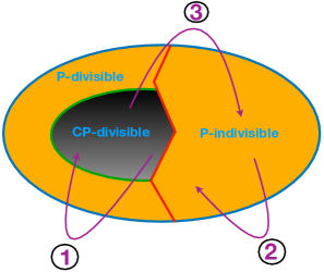
One can notice simply from the definitions of P- and CP-divisible quantum dynamics that all CP-divisible quantum dynamics will also be P-divisible; however, the reverse is not true. Therefore, we can split up all of the quantum dynamics into two groups: P-divisible and P-indivisible. Among the set of P-divisible dynamics, we can find dynamics that are also CP-divisible. To provide a visual idea of these categories, in Fig. 1, we draw a schematic diagram describing the different classes of quantum dynamics discussed above. In the figure, the red solid zigzag line differentiates P-divisible dynamics from P-indivisible ones, and the black portion shows CP-divisible dynamics. The region outside of the black portion represents CP-indivisible dynamics. In the next part of the paper, we offer an example where the dynamics found by operating the UQS on two CP-indivisible dynamics is CP-indivisible. Moreover, we state a necessary and sufficient condition for the indefinite causal order of two CP-divisible dynamics, modeled by the CQS, to be CP-divisible. Also, a few examples of pairs of CP-divisible dynamics are presented that become P-indivisible when acted on in indefinite causal order, again modeled by the CQS. These results are symbolically depicted using the purple arrows in Fig. 1. There can be other examples also for which, say the action of the switch may map P-divisible maps to
Before going into the details of the results, let us first discuss the tools we need to arrive at them.
We begin by providing a discussion on the detection of the P-indivisibility of quantum dynamics.
Detection of P-indivisibility Laine et al. (2010): When two different states of a system are affected by any fixed P-divisible dynamics, the distinguishability between the states either decreases or remains the same but never increases with time. Utilizing this characteristic of P-divisible dynamics, the BLP measure was introduced Laine et al. (2010), which can quantify the P-indivisibility of quantum dynamics.
In this paper, we will not exactly measure the P-indivisibility of any dynamics. Our aim will always be to detect P-indivisibility of quantum dynamics. As we just mentioned, if a quantum dynamics, say , of a particular system is P-divisible, then the distinguishability between the states, and , will monotonically decrease with time, , for any two initial states, and , of the system. Hence the trace distance, , between the states, and ,
will never increase with time, . In other words, P-divisible quantum dynamics, , imply
| (8) |
for any and any pair of states, and . Hence if a quantum dynamics violate the above inequality for any pair of times, , and states, , then the quantum dynamics is certainly P-indivisible.
For completeness, let us briefly define the trace distance. The trace distance between two states, and , acting on the same Hilbert space, can be expressed as
where , for any matrix , denotes .
In the next part, which is the last part of this section, we will discuss the conventional quantum switches.
Conventional Quantum Switches Chiribella et al. (2013b): Quantum switches are supermaps which take two or more quantum dynamics and create a superposition of different causal orders of them. We will denote the action of a quantum switch as . As the simplest non-trivial case, we consider quantum switches that are able to superpose causal orders of two quantum dynamics, say and . Let both of these channels act on a system which is initially prepared in the state . Typically a control system is required in order to build a quantum switch. Since we focus on the superposition of causal orders of two quantum dynamics, the corresponding control system needs to have at least dimension two. Let us assume that when the control is in the state , the quantum map, , acts on the state of the system, followed by the operation of the quantum map , and the channels act in the opposite order, i.e., the composite map, , acts on the state of the system when the control is in the state . Hence the state of the system first evolves for time to and then to . These are the two possible causal orders of the pair of dynamics.
Here and are elements of the two-dimensional computational basis of the Hilbert space, , which describes the control qubit. We consider to be the eigenbasis of .
Let us consider the initial states of the control qubit and the system to be and respectively. Then the action of the dynamics, created by applying a quantum switch, , on the two quantum dynamics, and , will transform the state, , as
| (9) |
where and are Kraus operators of the maps and , respectively and is the normalization coefficient. Here takes values and representing the two dynamics, and , and is element of . Since the map, , involves the action of two consecutive maps, the total time for which the system evolves under the entire process is to . We will denote the map which transfers to , constructed using the quantum switch, , as . The action of the map on a state, , will be denoted as . Though the exact form of the map also depends on the state of the control qubit, , and the parameter, , we are not explicitly including them in the notation, , for the sake of simplicity. The fourth argument of the function, , denotes the time of the application of the map, , on the system-control state, which in this scenario is considered to be 0.
One can generalize the definition of a quantum switch acting on two quantum dynamics to define quantum switches which act on quantum dynamics by considering a control system of dimension .
We will present another model of a quantum switch in the next section, named the universal quantum switch. The motivation behind the introduction of the quantum switch will also be discussed.
III Universal Quantum Switches
Before going into the details of the construction of a universal quantum switch, let us first discuss the need to introduce a new quantum switch.
Let us consider a situation where a system, , interacts with its environment, , for time to . Moreover, consider the interaction to be of two possible types, and the evolution of due to these two types of interactions be either described by a unitary, , or . The initial states of and are such that CPTP maps, and , can describe the evolution of resulting from the unitaries, and , respectively. For simplicity, let us consider the initial state of to be a product.
We first try to apply the conventional quantum switch, , to this pair of evolutions, and . In this regard, let us divide the whole time range, , into two parts, i.e., and , and introduce a control qubit. When the state of the control qubit is (), () acts on . The dynamics, and , being any arbitrary pair of CPTP evolutions, may not, in general, be CP-divisible. Therefore, even though the dynamics, and , are CPTP, the maps, and , may not have Kraus operator decomposition. One can notice from Eq. (9) that without Kraus operators, we can not define quantum switches in the usual way. Therefore, to define the superposition of different causal orders of CPTP dynamics, one or more of which are CP-indivisible, we need a quantum switch, which is not defined in terms of Kraus operators.
To understand the reason behind the difficulty in operating the conventional quantum switch in a more detailed way, let us discuss the scenario more elaborately. When the control qubit is, say, in state , as we mentioned above, the map acts on , i.e., first evolves under the unitary and then under . Since initially is in a product state, the first evolution of between is CPTP. But during this interaction, and may have generated a quantum correlation between them, due to which the evolution of in the time range will no longer be CPTP. Hence, the evolution of from to may not be expressible in terms of Kraus operators. Instead, if we had introduced another new separate environment, , at time , and evolved with unitary , then the new map, , describing the evolution of the system within time , would have been CPTP. Therefore, in such a scenario, the CQS could have been utilized. In this article, our purpose is to not introduce any new environment, , and create an indefinite causal order of interactions of with the same environment, . Therefore, we construct the universal quantum switch, , that can be used to create a superposition of causal orders of any quantum channels, and , including CP-indivisible ones.
Let us now move to the construction of . We consider the initial state of the system to be and denote the Hilbert space of the system as . For ease of understanding, we focus on systems of dimension two, but the method of applying on dynamics can easily be generalized for higher-dimensional systems. and represent the sequential action of the quantum dynamics, and , on the state , in the two possible causal orders. Let both and act on the same Hilbert space, , of dimension two. We denote the action of the UQS on and as . To apply on , we need to follow the steps presented below:
-
1.
Determine the spectral decomposition of each of the quantum states: and . Here () and () represent, respectively, the eigenvalues and eigenstates of ().
-
2.
Find a basis that has a maximum overlap with both the spectral bases, and . This can be realized by finding the maxima of the following function:
(10) over all pure states, , present in the Hilbert space, . Here denotes any pure state orthogonal to . Since the dimension of is two, the set will form a basis of . Let us denote the optimum basis for which attains its maximum value as .
-
3.
Finally, we can construct two states as follows:
(11) and
(12)
Since the above states are found by constructing a basis that has maximum overlap with the eigenbases of both and , we consider these states, and , as the final states, obtained by acting on the state .
As one can notice, the action of on the state, , has two definitions: one providing the state, , and the other resulting in the state, . Since and may not be unique, the pair of states, and , may also not be unique. Each and every one of these states will represent the action of on .
We would like to note here that the states and can be determined without using the channel’s Kraus decomposition. Hence, the construction of the UQS of any two or more quantum dynamics neither requires knowledge about the Kraus operators of any maps nor an external control system, like in the case of the CQS. Thus, we can construct a UQS for all quantum dynamics.
Here we have defined the UQS in such a way that it acts on two dynamics, and , but the method can easily be generalized to form a UQS that can act on any arbitrary but fixed number of dynamics.
In the upcoming section, we will present an example where the UQS can be seen to be outperforming the CQS.
IV Universal quantum switch provides an advantage in a state discrimination task
In this section, we will discuss a state discrimination task in which, in certain parameter regions, the UQS will be witnessed to provide more advantages than the CQS. Let us consider the following scenario: Alice prepares a single-qubit state, . She has a phase damping channel, , with noise strength , and a unitary channel, , which acts on two-dimensional systems. To avoid confusion, we would like to mention here that the number inside the braces in represents the noise strength of the channel and not the time for which the evolution is taking place. In this scenario, Alice tosses a coin; if she gets the head, she applies both and ; otherwise, she operates only on the state . She sends the final output state to Bob. Bob’s task is to determine if the unitary has acted upon the state by performing measurements on the received state. In these cases, when the result of the coin-toss is head, Alice can perform and on either in a definite causal order or in an indefinite causal order. The operation of and in indefinite causal order can again be implemented in two methods, viz., using the CQS or UQS. The exact difference between these three possible scenarios can be more clearly understood from the discussion below:
-
•
Definite causal order: In this case, if the coin is head, Alice sends , and if it is tail, she sends to Bob.
-
•
Conventional quantum switch: In this scenario, Alice transfers either the state, or depending on the result of the coin toss, where is the state of the control qubit. If the coin is head, she prepares and sends , and otherwise, she sends . See Eq. (9) for more detail on the functional form of .
-
•
Universal quantum switch: Here, if the coin is tail, Alice simply sends the state to Bob. Otherwise, Alice prepares the indefinite causal order of the two channels under consideration, i.e., and , following the model of the UQS, and acts the resulting map on . Specifically, she prepares the state , where is the basis for which , defined in Eq. (10), reaches its maximum value. Here is the set of eigenvalues of .
Bob has knowledge about which state he would receive if Alice got a head in the coin toss and what state he would get in the case of a tail. Nevertheless, Bob does not have any information about the exact result of the coin toss. After receiving the state, Bob tries to find out if Alice got a head or tail, i.e., Bob, knowing , tries to discriminate between the pair of states , where DCO, CQS, or UQS.
Bob follows the minimum error state discrimination protocol to distinguish the states. The minimum probability of error in discriminating any two states using the minimum error state discrimination method has already been found, and it is generally known as the Helstrom bound Helstrom (1969); Chefles (2000); Barnett (2001); Paris and Řeháček (2004); Bergou (2007); Barnett and Croke (2009); Bae and Kwek (2015). If two states, say and , are prepared with the probability and , respectively, the Helstrom bound tells us that the minimum probability of incorrectly guessing the state is . We can utilize the Helstrom bound to determine the minimum probability of error in distinguishing the states for all .
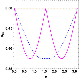
Considering the coin of Alice to be unbiased, , and
where is a constant, in Fig. 2, we depict the behavior of the minimum probability of error in the state discrimination protocol against . Specifically, in the figure, we plot , and using dashed-dotted orange line, dashed blue line, and solid pink line, respectively. From the plot, it can be noticed that there exist two wide ranges of , i.e., and for which is the smallest among the three error probabilities. Therefore, within these ranges, the application of and in indefinite causal order defined using the method of the UQS provides the most advantage compared to the other cases. Thus, we realize that in certain circumstances, the UQS can exhibit a benefit over the CQS.
V universal quantum switch can retain CP-indivisibility when acting upon CP-indivisible maps
In this section, we will form an indefinite causal order of two CP-indivisible dynamics using a quantum switch and show that the resulting dynamics remains CP-indivisible. In this regard, let us take a composite set-up consisting of a system, , and an environment, . We consider both of them to have dimension two. Let the initial state of the environment be , which is in product with the system, . At a moment, the system begins to interact with the environment. Hence, the entire set-up, , starts to unitarily evolve with time. Let there be two unitaries, and , which dictate the evolution of for the time interval . Here represents Planck’s constant. The two Hamiltonians, and , are given by
where and . Since the considered unitaries are entangling, the effective evolution of the system, , will certainly not be unitary. Let us denote the system’s evolution due to the interaction strengths, and , within time , as and . Considering the two following initial states of the system
and fixing the initial state of the environment at , we can calculate . From it can be easily checked using the P-divisibility criteria, discussed in Sec. II, that is P-indivisible for both and 2. Since P-indivisibility implies CP-indivisibility, we can conclude both and are CP-indivisible as well.
We want to find the indefinite causal order of the two dynamics, and , on the system, . In this regard, we divide the entire time range, , into two parts, viz., and . Within the two time intervals, the system interacts with the same environment with different strengths, either or . We will refer to the maps acting on the system between time and because of the system’s interaction with of strengths and , as and , respectively. One needs to keep in mind that, since at time , may be entangled with , the maps, and , may not be CPTP and therefore will not have any Kraus operator decomposition. Therefore, we cannot use CQS to generate the indefinite causal order of dynamics. Hence, we will use the UQS to form the indefinite causal orders of the two dynamics, and .
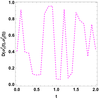
To examine if is CP-indivisible, we consider the same initial states, and , of the system, , and environment, . We first evaluate the states: and for and 2, and find their spectral decompositions. Finally, using their eigen decomposition, we determine and and denote them as and , respectively. Hence, and are the final states after the action of on and , respectively. We would like to mention here that the explicit forms of the states, and , depend on the time parameters, and . Considering and , in Fig. 3, we plot , as a function of . It is noticeable from the figure that there are various instances when increases with , indicating the non-monotonic behavior of . Hence, it can be concluded that the dynamics, , is CP-indivisible.
VI When do quantum switches preserve CP-divisibility?
In this section, we investigate the necessary and sufficient condition for the indefinite causal orders of two arbitrary CP-divisible dynamics, and , to be CP-divisible. We would like to note here that since () is CP-divisible, () will always have Kraus operator decomposition for all . Hence to prepare the indefinite causal order we can utilize the CQS, . We focus on the condition of the dynamics, , created by acting on the CP-divisible dynamics, and , to be CP-divisible. We also provide two examples of pairs of CP-divisible dynamics first of which remains CP-divisible when a CQS acts on them and the other becomes CP-indivisible when inserted in the CQS. Furthermore, we discuss examples of pairs of CP-divisible dynamics on which, when a CQS acts, the resulting dynamics not only becomes CP-indivisible but also P-indivisible.
We know, the dynamics, , constructed by applying the CQS on two CP-divisible dynamics, and , will be referred to as CP-divisible, if and only if
| (13) | |||
holds for each and every time and all quantum states, , with a control qubit, , where is a complete positive map.
In the next part, we state and prove the necessary and sufficient condition for the dynamics, , built by acting the CQS on two arbitrary CP-divisible dynamics, and , to be CP-divisible.
Theorem 1.
The dynamics, , constructed by applying the CQS on two CP-divisible dynamics, and , is CP-divisible, if and only if, the Kraus operators, and , of and that describe the evolution of the system, respectively, in between the time, , and , , satisfy
| (14) |
for all , , , , that obey . Here takes two values, 0 and 1, representing the two different dynamics, and .
Proof.
The exact expressions of and are given in the Appendix, where is the initial state of the system under consideration. If Eq. (14) be fulfilled by all the Kraus operators of the maps, and , for all , , , and and 2, it is evident that the requirements, mentioned in Eq. (VI), for the action of the CQS on two CP-divisible dynamics to be CP-divisible will be satisfied. Hence, it proves that Eq. (14) acts as a sufficient condition for the action of the CQS on two CP-divisible dynamics to provide a CP-divisible dynamics.
Let us now move to the necessary condition. In this regard, we consider the dynamics, , to be CP-divisible. Hence, , must be CPTP for all intermediate times, , which satisfy . Therefore, we can write
for all valid states, , of the system, , where is a set of Kraus operators. Substituting the exact expression of (written in the Appendix) in the left-hand side of the above equation and taking trace on both sides, we have
Here we have used the fact that and are two CP-divisible dynamics. Since the above equation is true for all , we can conclude that
where represents the identity operator which acts on the system’s Hilbert space. By simplifying the above expression we get
where . From the above equation, we can write , where is the th eigenvalue of . Hence we get for all , , , which implies for all and . Therefore we have
Thus we get the condition expressed in Eq. (14), is necessary to hold for the dynamics, , to be CP-divisible. Hence it completes the proof. ∎
Remark 1. Despite the fact that the Kraus operator decomposition of any CPTP map is not unique A. and Chuang (2010), the action of the CQS on two CPTP dynamics remains unique, whatever the considered Kraus decomposition of the maps that are participating in the switch Chiribella et al. (2013b). Since different Kraus operator decompositions of CPTP maps are unitarily connected with each other A. and Chuang (2010), if Eq. (14) holds for particular Kraus operator decompositions of a pair of maps, it will be satisfied for all Kraus operator decompositions of those pair of maps. Therefore, the stated necessary and sufficient condition does not depend on which set of Kraus operators is being considered.
Remark 2. The theorem can be generalized for any CQS that acts on an arbitrary but fixed number of CP-divisible dynamics. If we act CQS on CP-divisible dynamics, the resulting dynamics will form a superposition of causal orders of the input dynamics. Hence, the satisfaction of the commutativity relation, as expressed in Eq. (14), among Kraus operators of each and every pair of the set of maps, for all times, jointly serves as a necessary and sufficient criterion for maintaining CP-divisibility of the dynamics created by applying the CQS on CP-divisible dynamics.
Let us now come to some examples. The first example is of a dynamics generated by acting the CQS on two phase damping channels. Since the Kraus operators, , , and , of two ideal phase damping channels satisfy Eq. (14), where and are the Lindblad coefficients of the channels, we arrive at the following conclusion:
Example 1.
The dynamics produced by applying the CQS on two phase damping channels is CP-divisible.
One can notice from the expressions presented in Eqs. (4) and (7) that the Kraus operators of the amplitude damping channel do not commute with each other. Hence, they do not satisfy Eq. (14). Therefore, we get
Example 2.
The dynamics formed by applying the CQS on two ideal amplitude damping channels is CP-indivisible.
The examples assure that the fulfillment of the necessary and sufficient condition given in Eq. (14) can be easily verified for quantum dynamics.
Let us now try to check if it is possible to prepare the P-indivisible dynamics by operating the CQS on pairs of CP-divisible dynamics. We will make use of Eq. (8) to detect the P-indivisibility of the dynamics constructed by the CQS. In all the examples discussed below, to apply the CQS using the definition given in Eq. 9, we take and , where is the half of the total evolution time of the system.
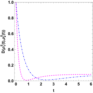
We know an ideal depolarizing channel is CP-divisible. Regardless of whether we consider the Lindblad coefficients of a pair of depolarizing channels to be the same or different, the Kraus operators of the channels are not going to commute. Therefore, according to Theorem 1, the operation of CQS on any two depolarizing channels will produce CP-indivisible dynamics. Let us further check if the produced dynamics is P-indivisible. In this regard, we take two initial states, and , of a system on which the depolarizing channels can act. First, we consider the two depolarizing channels to have equal Lindblad coefficients, .
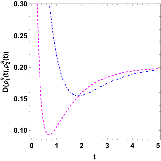
We evaluate and and plot the trace distance, , between and with time, , in Fig. 4, using blue dash-dotted curve. One can notice from the curve that shows non-monotonic behavior with respect to . This characteristic proves that the operation of the CQS on two depolarizing channels with the same Lindblad coefficients can produce P-indivisible dynamics. Next, we apply the CQS on two depolarizing channels having unequal Lindblad coefficients, i.e., one with and the other with . For these two considered depolarizing channels, we again plot the trace distance, , in Fig. 4, using a pink dashed line, where and . In this scenario also, we can notice a non-monotonic behavior in the pink dashed curve with respect to time, , proving the P-indivisible nature of the dynamics, . Hence, we get to the following conclusion:
Example 3.
The action of the CQS on two CP-divisible dynamics, which are ideal depolarizing channels having the same or different Lindblad coefficients, can produce a P-indivisible dynamics.
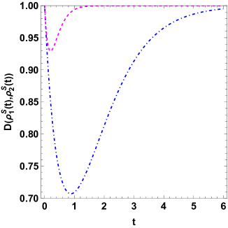
We also apply the CQS on two pairs of channels, viz., ideal depolarizing and amplitude damping channels having the same Lindblad coefficients, , and the same pair of channels having unequal Lindblad coefficients, i.e., and . Since the Kraus operators of the depolarizing maps do not commute with the same of amplitude damping channels in both situations, the effective dynamics created by the CQS will be CP-indivisible. We can verify the P-indivisibility of the dynamics, in the same way as in the previous example. In this regard, we consider the same initial states, and . In Fig. 5, we illustrate the trace distances, , between the states and for the cases where the Lindblad coefficients have equal values (dash-dotted blue line) and unequal values (dashed pink line) with respect to . The clear non-monotonic nature of the curves over for both cases confirms the following result:
Example 4.
The dynamics produced by applying the CQS on two CP-divisible dynamics, viz., ideal amplitude damping and depolarizing channels having the same or different Lindblad coefficients, can be P-indivisible.
As the final example, in Fig. 6, we plot the trace distance, , between and , where and are the same initial states as considered in the previous two examples. The blue dash-dotted and pink dashed curves depict scenarios where the two channels, and , have equal Lindblad coefficients, and unequal Lindblad coefficients, i.e., and , respectively. From the non-monotonic behaviors of with respect to , which can be clearly witnessed in the two curves of Fig. 6, we make the following statement:
Example 5.
The operation of the CQS on two CP-divisible dynamics, the ideal depolarizing and phase-damping channels having the same or different Lindblad coefficients, can create a P-indivisible dynamics.
VII conclusion
A quantum switch is a superoperator that creates a superposition of different causal orders of quantum channels using a control system. In quantum informational tasks, dynamics generated by applying a quantum switch on two channels have been proven to provide advantage over the utilization of the channels in definite causal order.
Due to the inability to decompose the intermediate evolution of a system undergoing CP-indivisible dynamics into Kraus operators, the operation of a traditional quantum switch on CP-indivisible dynamics is infeasible. We provided the notion of a universal quantum switch that can be applied on all types of quantum dynamics. Our approach allowed for the construction of the indefinite causal order of any set of quantum dynamics without limiting it to CP-divisible dynamics. We further presented a state discrimination task where the UQS was proven to perform better than the usual quantum switch in certain parameter regions. Using the model of the UQS, we showed an example where the indefinite causal order of two CP-indivisible channels is CP-indivisible. Moreover, we investigated whether the typical quantum switch can preserve CP-divisibility when superposing the different causal orders of CP-divisible dynamics. We analytically proved that the commutativity of the Kraus operators of one of the CP-divisible channels with the Kraus operators of the other CP-divisible channel for all time is a necessary and sufficient criterion for the channel generated by the action of the CQS on these channels to be CP-divisible. Finally, we found a few examples of CP-divisible dynamics transforming into P-indivisible dynamics when acted upon by the typical quantum switch.
Acknowledgment
KS acknowledges support from the project MadQ-CM (Madrid Quantum de la Comunidad de Madrid) funded by the European Union (NextGenerationEU, PRTR-C17.I1) and by the Comunidad de Madrid (Programa de Acciones Complementarias).
Appendix
Let us assume that and are the Kraus operators of the two maps, and , that evolves the system from any initial time, , to a final time, . Here we have considered the state of the control as .
where . Then, we can write as follows:
for .
References
- Rivas and Huelga (2012) Á Rivas and S. F. Huelga, Open Quantum Systems (Springer Berlin Heidelberg, 2012).
- Rivas et al. (2014) Á Rivas, S. F. Huelga, and M. B. Plenio, “Quantum non-Markovianity: characterization, quantification and detection,” Rep. Prog. Phys. 77, 094001 (2014).
- Breuer et al. (2016) H-P. Breuer, E-M. Laine, J. Piilo, and B. Vacchini, “Colloquium: Non-Markovian dynamics in open quantum systems,” Rev. Mod. Phys. 88, 021002 (2016).
- de Vega and Alonso (2017) I. de Vega and D. Alonso, “Dynamics of non-Markovian open quantum systems,” Rev. Mod. Phys. 89, 015001 (2017).
- Vasile et al. (2011) R. Vasile, S. Olivares, M. A. Paris, and S. Maniscalco, “Continuous-variable quantum key distribution in non-Markovian channels,” Phys. Rev. A 83, 042321 (2011).
- Chen et al. (2016) P. Chen, M. M. Ali, and S. Chen, “Enhanced quantum nonlocality induced by the memory of a thermal-squeezed environment,” Journal of Physics A: Mathematical and Theoretical 49, 395302 (2016).
- Gupta et al. (2022) R. Gupta, S. Gupta, S. Mal, and A. Sen(De), “Constructive feedback of non-Markovianity on resources in random quantum states,” Phys. Rev. A 105, 012424 (2022).
- Roy et al. (2023) P. Roy, S. Bera, S. Gupta, and A. S. Majumdar, “Device-independent quantum secure direct communication under non-Markovian quantum channels,” arXiv:2312.03040 (2023).
- Muhuri et al. (2024) A. Muhuri, R. Gupta, S. Ghosh, and A. Sen(De), “Superiority in dense coding through non-Markovian stochasticity,” Phys. Rev. A 109, 032616 (2024).
- Chen et al. (2023) Y-Q. Chen, S-X. Zhang, and S. Zhang, “Non-Markovianity benefits quantum dynamics simulation,” arXiv:2311.17622 (2023).
- Bylicka et al. (2016) B. Bylicka, M. Tukiainen, D. Chruściński, J. Piilo, and S. Maniscalco, “Thermodynamic power of non-markovianity,” Scientific Reports 6, 27989 (2016).
- Ghoshal et al. (2021) A. Ghoshal, S. Das, A. K. Pal, A. Sen(De), and U. Sen, “Three qubits in less than three baths: Beyond two-body system-bath interactions in quantum refrigerators,” Phys. Rev. A 104, 042208 (2021).
- Ghosh et al. (2021) S. Ghosh, T. Chanda, S. Mal, and A. Sen(De), “Fast charging of a quantum battery assisted by noise,” Phys. Rev. A 104, 032207 (2021).
- Ghoshal and Sen (2022) A. Ghoshal and U. Sen, “Heat current and entropy production rate in local non-Markovian quantum dynamics of global Markovian evolution,” Phys. Rev. A 105, 022424 (2022).
- Ptaszyński (2022) K. Ptaszyński, “Non-markovian thermal operations boosting the performance of quantum heat engines,” Phys. Rev. E 106, 014114 (2022).
- Sen and Sen (2023) K. Sen and U. Sen, “Noisy quantum batteries,” arXiv:2302.07166 (2023).
- Tang et al. (2024) H. Tang, Y. Guo, X. Hu, Y. Huang, B. Liu, C. Li, and G. Guo, “Demonstration of superior communication through thermodynamically free channels in an optical quantum switch,” arXiv:2406.02236 (2024).
- Rivas et al. (2010) Á. Rivas, S. F. Huelga, and M. B. Plenio, “Entanglement and non-Markovianity of quantum evolutions,” Phys. Rev. Lett. 105, 050403 (2010).
- Laine et al. (2010) E. Laine, J. Piilo, and H-P. Breuer, “Measure for the non-Markovianity of quantum processes,” Phys. Rev. A 81, 062115 (2010).
- Oreshkov et al. (2012) O. Oreshkov, F. Costa, and Č. Brukner, “Quantum correlations with no causal order,” Nat. Commun. 3, 1092 (2012).
- Chiribella et al. (2013a) G. Chiribella, G. M. D’Ariano, P. Perinotti, and B. Valiron, “Quantum computations without definite causal structure,” Phys. Rev. A 88, 022318 (2013a).
- Brukner (2014) Č Brukner, “Quantum causality,” Nature Physics , 259 (2014).
- Araújo et al. (2015) M. Araújo, C. Branciard, F. Costa, A. Feix, C. Giarmatzi, and C. Brukner, “Witnessing causal nonseparability,” New Journal of Physics 17, 102001 (2015).
- Oreshkov and Giarmatzi (2016) O. Oreshkov and C. Giarmatzi, “Causal and causally separable processes,” New Journal of Physics 18, 093020 (2016).
- Chiribella et al. (2013b) G. Chiribella, G. M. D’Ariano, P. Perinotti, and B. Valiron, “Quantum computations without definite causal structure,” Phys. Rev. A 88, 022318 (2013b).
- Chiribella (2012) G. Chiribella, “Perfect discrimination of no-signalling channels via quantum superposition of causal structures,” Phys. Rev. A 86, 040301 (2012).
- Bavaresco et al. (2022) J. Bavaresco, M. Murao, and M. T. Quintino, “Unitary channel discrimination beyond group structures: Advantages of sequential and indefinite-causal-order strategies,” Journal of Mathematical Physics 63, 042203 (2022).
- Guérin et al. (2016) P. A. Guérin, A. Feix, M. Araújo, and Č. Brukner, “Exponential communication complexity advantage from quantum superposition of the direction of communication,” Phys. Rev. Lett. 117, 100502 (2016).
- Ebler et al. (2018) D. Ebler, S. Salek, and G. Chiribella, “Enhanced communication with the assistance of indefinite causal order,” Phys. Rev. Lett. 120, 120502 (2018).
- Mukhopadhyay and Pati (2020) C. Mukhopadhyay and A. K. Pati, “Superposition of causal order enables quantum advantage in teleportation under very noisy channels,” J. Phys. Commun. 4, 105003 (2020).
- Chiribella et al. (2021) G. Chiribella, M. Banik, S. S. Bhattacharya, T. Guha, M. Alimuddin, A. Roy, S. Saha, S. Agrawal, and G. Kar, “Indefinite causal order enables perfect quantum communication with zero capacity channels,” New Journal of Physics 23, 033039 (2021).
- Rubino et al. (2021) G. Rubino, L. A. Rozema, D. Ebler, H. Kristjánsson, S. Salek, P. Allard Guérin, A. A. Abbott, C. Branciard, Č. Brukner, G. Chiribella, and P. Walther, “Experimental quantum communication enhancement by superposing trajectories,” Phys. Rev. Res. 3, 013093 (2021).
- Zhao et al. (2020a) X. Zhao, Y. Yang, and G. Chiribella, “Quantum metrology with indefinite causal order,” Phys. Rev. Lett. 124, 190503 (2020a).
- Zhao et al. (2020b) X. Zhao, Y. Yang, and G. Chiribella, “Quantum metrology with indefinite causal order,” Phys. Rev. Lett. 124, 190503 (2020b).
- Chapeau-Blondeau (2021) F. Chapeau-Blondeau, “Noisy quantum metrology with the assistance of indefinite causal order,” Phys. Rev. A 103, 032615 (2021).
- Xie et al. (2021) D. Xie, C. Xu, and A. Wang, “Quantum metrology with coherent superposition of two different coded channels,” Chin. Phys. B 30, 090304 (2021).
- Chapeau-Blondeau (2022) F. Chapeau-Blondeau, “Indefinite causal order for quantum metrology with quantum thermal noise,” Phys. Lett. A 447, 128300 (2022).
- Ban (2023) M. Ban, “Quantum fisher information of phase estimation in the presence of indefinite causal order,” Physics Letters A 468, 128749 (2023).
- An et al. (2024) M. An, S. Ru, Y. Wang, Y. Yang, F. Wang, P. Zhang, and F. Li, “Noisy quantum parameter estimation with indefinite causal order,” Phys. Rev. A 109, 012603 (2024).
- Felce and Vedral (2020) D. Felce and V. Vedral, “Quantum refrigeration with indefinite causal order,” Phys. Rev. Lett. 125, 070603 (2020).
- Jifei and Youyang (2022) Z. Jifei and X. Youyang, “Influence of an indefinite causal order on an otto heat engine,” Communications in Theoretical Physics 74, 025601 (2022).
- Cao et al. (2022) H. Cao, N. Wang, Z. Jia, C. Zhang, Y. Guo, B. Liu, Y. Huang, C. Li, and G. Guo, “Quantum simulation of indefinite causal order induced quantum refrigeration,” Phys. Rev. Research 4, L032029 (2022).
- Nie et al. (2022) X. Nie, X. Zhu, K. Huang, K. Tang, X. Long, Z. Lin, Y. Tian, C. Qiu, C. Xi, X. Yang, J. Li, Y. Dong, T. Xin, and D. Lu, “Experimental realization of a quantum refrigerator driven by indefinite causal orders,” Phys. Rev. Lett. 129, 100603 (2022).
- Maity and Bhattacharya (2022) A. G. Maity and S. Bhattacharya, “Activating hidden non-Markovianity with the assistance of quantum SWITCH,” arXiv:2206.04524 (2022).
- Koudia and Gharbi (2019) S. Koudia and A. Gharbi, “Superposition of causal orders for quantum discrimination of quantum processes,” International Journal of Quantum Information 17, 1950055 (2019).
- Kunjwal and Baumeler (2023) Ravi Kunjwal and Ämin Baumeler, “Trading causal order for locality,” Phys. Rev. Lett. 131, 120201 (2023).
- Procopio et al. (2015) L. M. Procopio, A. Moqanaki, M. Araújo, F. Costa, I. Calafell, E. G. Dowd, D. R. Hamel, L. A. Rozema, Č. Brukner, and P. Walther, “Experimental superposition of orders of quantum gates,” Nat. Commun. 6, 7913 (2015).
- Rubino et al. (2017) G. Rubino, L. A. Rozema, A. Feix, M. Araújo, J. M. Zeuner, L. M. Procopio, Č. Brukner, and P. Walther, “Experimental verification of an indefinite causal order,” Sci. Adv. 3, e1602589 (2017).
- Goswami et al. (2018) K. Goswami, C. Giarmatzi, M. Kewming, F. Costa, C. Branciard, J. Romero, and A. G. White, “Indefinite causal order in a quantum switch,” Phys. Rev. Lett. 121, 090503 (2018).
- Taddei et al. (2021) M. M. Taddei, J. Cariñe, D. Martínez, T. García, N. Guerrero, A. A. Abbott, M. Araújo, C. Branciard, E. S. Gómez, S. P. Walborn, L. Aolita, and G. Lima, “Computational advantage from the quantum superposition of multiple temporal orders of photonic gates,” PRX Quantum 2, 010320 (2021).
- Rubino et al. (2022) G. Rubino, L. A. Rozema, F. Massa, M. Araújo, M. Zych, Č. Brukner, and P. Walther, “Experimental entanglement of temporal order,” Quantum 6, 621 (2022).
- A. and Chuang (2010) M. A. Nielsen M. A. and I. L. Chuang, Quantum Computation and Quantum Information (Cambridge University Press, 2010).
- Helstrom (1969) C. W. Helstrom, “Quantum detection and estimation theory,” J. Stat. Phys. 1, 231 (1969).
- Chefles (2000) A. Chefles, “Quantum state discrimination,” Contemporary Physics 41, 401 (2000).
- Barnett (2001) S. M. Barnett, “Quantum limited state discrimination,” Protein Science 49, 909 (2001).
- Paris and Řeháček (2004) M. Paris and J. Řeháček, Quantum State Estimation, Vol. 649 (Springer Science & Business Media, 2004).
- Bergou (2007) J. A. Bergou, “Quantum state discrimination and selected applications,” Journal of Physics: Conference Series 84, 012001 (2007).
- Barnett and Croke (2009) S. M. Barnett and S. Croke, “Quantum state discrimination,” Adv. Opt. Photon. 1, 238 (2009).
- Bae and Kwek (2015) J. Bae and L. Kwek, “Quantum state discrimination and its applications,” Journal of Physics A: Mathematical and Theoretical 48, 083001 (2015).