Finite Neural Networks as Mixtures of Gaussian Processes: From Provable Error Bounds to Prior Selection

Abstract

Infinitely wide or deep neural networks (NNs) with independent and identically distributed (i.i.d.) parameters have been shown to be equivalent to Gaussian processes. Because of the favorable properties of Gaussian processes, this equivalence is commonly employed to analyze neural networks and has led to various breakthroughs over the years. However, neural networks and Gaussian processes are equivalent only in the limit; in the finite case there are currently no methods available to approximate a trained neural network with a Gaussian model with bounds on the approximation error. In this work, we present an algorithmic framework to approximate a neural network of finite width and depth, and with not necessarily i.i.d. parameters, with a mixture of Gaussian processes with error bounds on the approximation error. In particular, we consider the Wasserstein distance to quantify the closeness between probabilistic models and, by relying on tools from optimal transport and Gaussian processes, we iteratively approximate the output distribution of each layer of the neural network as a mixture of Gaussian processes. Crucially, for any NN and $\epsilon>0$ our approach is able to return a mixture of Gaussian processes that is $\epsilon$-close to the NN at a finite set of input points. Furthermore, we rely on the differentiability of the resulting error bound to show how our approach can be employed to tune the parameters of a NN to mimic the functional behavior of a given Gaussian process, e.g., for prior selection in the context of Bayesian inference. We empirically investigate the effectiveness of our results on both regression and classification problems with various neural network architectures. Our experiments highlight how our results can represent an important step towards understanding neural network predictions and formally quantifying their uncertainty.

Keywords: Neural Networks, Gaussian Processes, Bayesian inference, Wasserstein distance

1 Introduction

Deep neural networks have achieved state-of-the-art performance in a wide variety of tasks, ranging from image classification (Krizhevsky et al., 2012) to robotics and reinforcement learning (Mnih et al., 2013). In parallel with these empirical successes, there has been a significant effort in trying to understand the theoretical properties of neural networks (Goodfellow et al., 2016) and to guarantee their robustness (Szegedy et al., 2013). In this context, an important area of research is that of stochastic neural networks (SNNs), where some of the parameters of the neural network (weights and biases) are not fixed, but follow a distribution. SNNs include many machine learning models commonly used in practice, such as dropout neural networks (Gal and Ghahramani, 2016), Bayesian neural networks (Neal, 2012), neural networks with only a subset of stochastic layers (Favaro et al., 2023), and neural networks with randomized smoothing (Cohen et al., 2019). Among these, because of their convergence to Gaussian processes, particular theoretical attention has been given to infinite neural networks with independent and identically distributed (i.i.d.) parameters (Neal, 2012; Lee et al., 2017).

Gaussian processes (GPs) are a class of stochastic processes that are widely used as non-parametric machine learning models (Rasmussen, 2003). Because of their many favorable analytic properties (Adler and Taylor, 2009), the convergence of infinite SNNs to GPs has enabled many breakthroughs in the understanding of neural networks, including their modeling capabilities (Schoenholz et al., 2016), their learning dynamics (Jacot et al., 2018), and their adversarial robustness (Bortolussi et al., 2024). Unfortunately, existing results to approximate a SNN with a GP are either limited to untrained networks with i.i.d. parameters (Neal, 2012) or lack guarantees of correctness (Khan et al., 2019). In fact, the input-output distribution of a SNN of finite depth and width is generally non-Gaussian, even if the distribution over its parameters is Gaussian (Lee et al., 2020). This leads to the main question of this work: Can we develop an algorithmic framework to approximate a finite SNN (trained or untrained and not necessarily with i.i.d. parameters) with Gaussian models while providing formal guarantees of correctness (i.e., provable bounds on the approximation error and that can be made arbitrarily small)?

In this paper, we propose an algorithmic framework to approximate the input-output distribution of an arbitrary SNN over a finite set of input points with a Gaussian Mixture Model (GMM), that is, a mixture of $M$ Gaussian distributions (McLachlan and Peel, 2000). Critically, the GMM approximation resulting from our approach comes with error bounds on its distance (in terms of the 2-Wasserstein distance (Villani et al., 2009)) to the input-output distribution of the SNN. An illustrative example of our framework is shown in Figure 1(a), where, given a SNN trained on a 1D regression task (Figure 1(a)), our framework outputs a GMM approximation (Figure 1(b)) with error bounds on its closeness to the SNN (Figure 1(c)). Our approach is based on iteratively approximating the output distribution of each layer of the SNN with a mixture of Gaussian distributions and propagating this distribution through the next layer. In order to propagate a distribution through a non-linear activation function, we first approximate it with a discrete distribution, which we call a signature approximation. The resulting discrete distribution can then be propagated exactly through a layer of the neural network (activation function and linear combination with weights and biases), which in the case of jointly Gaussian weights and biases, leads to a new Gaussian mixture distribution. To quantify the error between the SNN and the resulting GMM, we use techniques from optimal transport, probability theory, and interval arithmetic. In particular, for each of the approximation steps described above, we bound the error introduced in terms of the 2-Wasserstein distance. Then, we combine these bounds using interval arithmetic to bound the 2-Wasserstein distance between the SNN and the approximating GMM. Furthermore, by relying on the fact that GMMs can approximate any distribution arbitrarily well (Delon and Desolneux, 2020), we prove that by appropriately picking the parameters of the GMM, the bound on the approximation error converges uniformly to zero by increasing the size of the GMM. Additionally, we show that the resulting error bound is piecewise differentiable in the hyper-parameters of the neural network, which allows one to optimize the behavior of a NN to mimic that of a given GMM via gradient-based algorithms.

(a) SNN

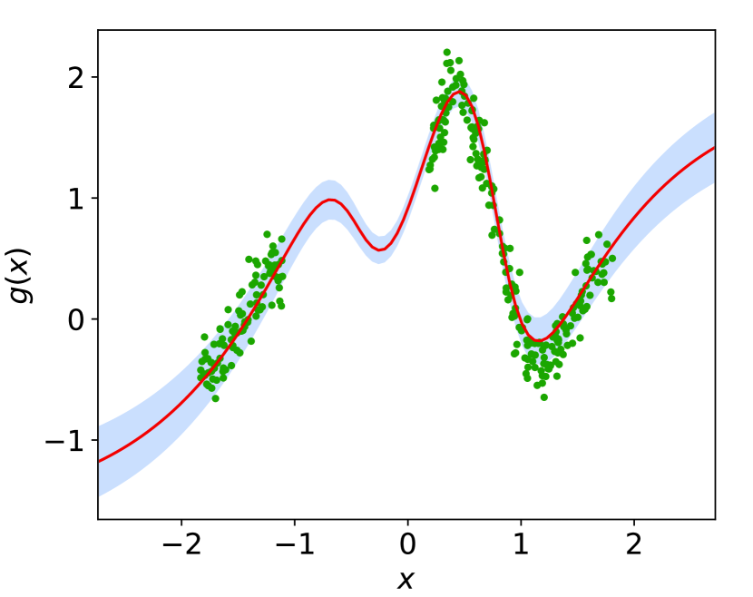
(b) GMM

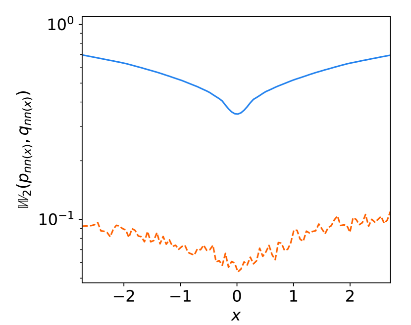
(c) Error

Figure 1: Visualization of (a) a Monte Carlo approximation of a SNN trained on samples from a 1D mixture of sines with additive noise, and (b) the GMM approximation of the same SNN composed of a mixture of size $10$, as obtained with our approach. The SNN has one hidden layer with 64 neurons and is trained using VOGN (Khan et al., 2018). The red line and blue-shaded region in (a) and (b) illustrate the point-wise mean and standard deviation at a uniform grid of 100 points in the input domain. In (c), the dashed and solid lines represent, respectively, the empirical estimates of the 2-Wasserstein distance between the GMM and SNN distributions at each input point, and formal bounds of the same quantity, as obtained by the results derived in this paper.

We empirically validate our framework on various SNN architectures, including fully connected and convolutional layers, trained for both regression and classification tasks on various datasets including MNIST, CIFAR-10, and a selection of UCI datasets. Our experiments confirm that our approach can successfully approximate a SNN with a GMM with arbitrarily small error, albeit with increasing computational costs when the network’s depth increases. Furthermore, perhaps surprisingly, our results show that even a mixture with a relatively small number of components generally suffices to empirically approximate a SNN accurately. To showcase the importance of our results, we then consider two applications: (i) uncertainty quantification in SNNs, and (ii) prior selection for SNNs. In the former case we show how the GMM approximation resulting from our framework can be used to study and quantify the uncertainty of the SNN predictions in classification tasks on the MNIST and CIFAR-10 datasets. In the latter case, we consider prior selection for neural networks, which is arguably one of the most important problems in performing Bayesian inference with neural networks (Fortuin, 2022), and show that our framework allows one to precisely encode functional information in the prior of SNNs expressed as Gaussian processes (GPs), thereby enhancing SNNs’ posterior performance and outperforming state-of-the-art methods for prior selection of neural networks.

In summary, the main contributions of our paper are:

• We introduce a framework based on discrete approximations of continuous distributions to approximate SNNs of arbitrary depth and width as GMMs, with formal error bounds in terms of the 2-Wasserstein distance.

• We prove the uniform convergence of our framework by showing that for any finite set of input points our approach can return a GMM of finite size such that the 2-Wasserstein distance between this distribution and the joint input-output distribution of the SNN on these points can be made arbitrarily small.

• We perform a large-scale empirical evaluation to demonstrate the efficacy of our algorithm in approximating SNNs with GMMs and to show how our results could have a profound impact in various areas of research for neural networks, including uncertainty quantification and prior selection.

1.1 Related Works

The convergence of infinitely wide SNNs with i.i.d. parameters to GPs was first studied by Neal (2012) by relying on the central limit theorem. The corresponding GP kernel for the one hidden layer case was then analytically derived by Williams (1996). These results were later generalized to deep NNs (Hazan and Jaakkola, 2015; Lee et al., 2017; Matthews et al., 2018), convolutional layers (Garriga-Alonso et al., 2019; Novak et al., 2018; Garriga-Alonso and van der Wilk, 2021), and general non-linear activation functions (Hanin, 2023). However, these results only hold for infinitely wide or deep neural networks with i.i.d. parameters; in practice, NNs have finite size and depth and for trained NNs their parameters are generally not i.i.d.. To partially address these issues, recent works have started to investigate how these results apply in the finite case (Dyer and Gur-Ari, 2019; Antognini, 2019; Yaida, 2020; Bracale et al., 2021; Klukowski, 2022; Balasubramanian et al., 2024). In particular, Eldan et al. (2021) were the first to provide upper bounds on the rates at which a single layer SNN with a specific parameter distribution converges to the infinite width GP in terms of the Wasserstein distance. This result was later generalized to isotropic Gaussian weight distributions (Cammarota et al., 2023), deep Random NN (Basteri and Trevisan, 2024), and to other metrics, such as the total variation, sup norm, and Kolmogorov distances (Apollonio et al., 2023; Bordino et al., 2023; Favaro et al., 2023). However, to the best of our knowledge, all existing works are limited to untrained SNNs with i.i.d. weights and biases, which may be taken as priors in a Bayesian setting (Bishop and Nasrabadi, 2006) or may represent the initialization of gradient flows in an empirical risk minimization framework (Jacot et al., 2018). In contrast, critically, in our paper we allow for correlated and non-identical distributed weights and biases, thus also including trained posterior distributions of SNNs learned via Bayesian inference. In this context, Khan et al. (2019) showed that for a subset of Gaussian Bayesian inference techniques, the approximate posterior weight distributions are equivalent to the posterior distributions of GP regression models, implying a linearization of the approximate SNN posterior in function space (Immer et al., 2021). Instead, we approximate the SNN with guarantees in function space and our approach generalizes to any approximate inference technique.

While the former set of works focuses on the convergence of SNNs to GPs, various works have considered the complementary problem of finding the distribution of the parameters of a SNN that mimic a given GP (Flam-Shepherd et al., 2017, 2018; Tran et al., 2022; Matsubara et al., 2021). This is motivated by the fact that GPs offer an excellent framework to encode functional prior knowledge; consequently, this problem has attracted significant interest in encoding functional prior knowledge into the prior of SNNs. In particular, closely related to our setting are the works of Flam-Shepherd et al. (2017) and Tran et al. (2022), which optimize the parametrization of the weight-space distribution of the SNN to minimize the KL divergence and 1-Wasserstein distance, respectively, with a desired GP prior. They then utilize the optimized weight prior to perform Bayesian inference, showing improved posterior performance. However, these methods lack formal guarantees on the closeness of the optimized SNN and the GP that the error bounds we derive in this paper provide.

2 Notation

For a vector ${{x}}\in{\mathbb{R}}^{n}$, we denote with $\|{{x}}\|$ the Euclidean norm on ${\mathbb{R}}^{n}$, and use ${{{x}}^{(i)}}$ to denote the $i$-th element of $x$. Similarly, for a matrix ${{M}}\in{\mathbb{R}}^{n\times m}$ we denote by $\|{{M}}\|$ the spectral (matrix) norm of ${{M}}$ and use ${{M}}^{(i,j)}$ to denote the $(i,j)$-th element of ${{M}}$. Further, ${{\bar{1}}}_{n}\in{\mathbb{R}}^{n}$ and ${{\bar{1}}}_{m\times n}\in{\mathbb{R}}^{m\times n}$, respectively, denote a vector and matrix of ones, and $I_{n}\in{\mathbb{R}}^{n\times n}$ is used to denote the identity matrix of size $n$. Given a linear transformation function (matrix) ${{T}}\in{\mathbb{R}}^{m\times n}$, the post image of a region ${\mathcal{X}}\subset{\mathbb{R}}^{n}$ under ${{T}}$ is defined as $\mathrm{Post}({\mathcal{X}},{{T}})=\{{{T}}{{x}}\mid{{x}}\in{\mathcal{X}}\}$. If ${\mathcal{X}}\subset{\mathbb{R}}^{n}$ is finite, we denote by $|{\mathcal{X}}|$ the cardinality of ${\mathcal{X}}$. Further, we define ${\mathbf{1}}_{\mathcal{X}}:{\mathbb{R}}^{n}\rightarrow\{0,1\}$ as the step function over region ${\mathcal{X}}\subset{\mathbb{R}}^{n}$, that is, ${\mathbf{1}}_{{\mathcal{X}}}({{x}})=\begin{cases}1&{{x}}\in{\mathcal{X}},\\ 0&\text{otherwise.}\end{cases}$

Given a measurable space $({\mathcal{X}},{\mathcal{B}}({\mathcal{X}}))$ with ${\mathcal{B}}({\mathcal{X}})$ being the $\sigma-$algebra, we denote with ${\mathcal{P}}({\mathcal{X}})$ the set of probability distributions on $({\mathcal{X}},{\mathcal{B}}({\mathcal{X}}))$. In this paper, for a metric space ${\mathcal{X}}$, ${\mathcal{B}}({\mathcal{X}})$ is assumed to be the Borel $\sigma$-algebra of ${\mathcal{X}}$. Considering two measurable spaces $({\mathcal{X}},{\mathcal{B}}({\mathcal{X}}))$ and $({\mathcal{Y}},{\mathcal{B}}({\mathcal{Y}}))$, a probability distribution $p\in{\mathcal{P}}({\mathcal{X}})$, and a measurable mapping $h:{\mathcal{X}}\rightarrow{\mathcal{Y}}$, we use $h\#p$ to denote the push-forward measure of $p$ by $h$, i.e., the measure on ${\mathcal{Y}}$ such that $\forall{\mathcal{A}}\in{\mathcal{Y}}$, $(h\#p)({\mathcal{A}}))=p(h^{-1}({\mathcal{A}}))$. For $N\in\mathbb{N}$, $\Pi_{N}=\{\pi\in{\mathbb{R}}^{N}_{\geq 0}:\sum^{N}_{i=1}{\pi^{{(i)}}}=1\}$ is the N-simplex. A discrete probability distribution $d\in{\mathcal{P}}({\mathcal{X}})$ is defined as $d=\sum_{i=1}^{N}{{{\pi}}^{(i)}}\delta_{{{c}}_{i}}$, where $\delta_{{c}}$ is the Dirac delta function centered at location ${{c}}\in{\mathcal{X}}$ and $\pi\in\Pi_{N}$. Lastly, the set of discrete probability distributions on ${\mathcal{X}}$ with at most $N$ locations is denoted as ${\mathcal{D}}_{N}({\mathcal{X}})\subset\mathcal{P}({\mathcal{X}})$.

3 Preliminaries

In this section, we give the necessary preliminary information on Gaussian models and on the Wasserstein distance between probability distributions.

3.1 Gaussian Processes and Gaussian Mixture Models

A Gaussian process (GP) $g$ is a stochastic process such that for any finite collection of input points ${\mathcal{X}}=\{{{x}}_{1},\ldots,{{x}}_{D}\}$ the joint distribution of $g({\mathcal{X}})\coloneqq\{g({{x}}_{1}),\ldots,g({{x}}_{D})\}$ follows a multivariate Guassian distribution with mean function ${m}$ and covariance function ${k}$, i.e., $g({\mathcal{X}})\sim\mathcal{N}({m}({\mathcal{X}})),{k}({\mathcal{X}},{\mathcal{X}}))$ (Adler and Taylor, 2009). A Gaussian Mixture Model (GMM) with $M\in\mathbb{N}$ components, is a set of $M$ GPs, also called components, averaged w.r.t. a probability vector $\pi\in\Pi_{M}$ (Tresp, 2000). Therefore, the probability distribution of a GMM follows a Gaussian mixture distribution.

Definition 1 (Gaussian Mixture Distribution)

A probability distribution $q\in{\mathcal{P}}({\mathbb{R}}^{d})$ is called a Gaussian Mixture distribution of size $M\in\mathbb{N}$ if $q=\sum_{i=1}^{M}{{{\pi}}^{{(i)}}}\mathcal{N}({m}_{i},\Sigma_{i}),$ where $\pi\in\Pi_{M}$ and ${m}_{i}\in{\mathbb{R}}^{d}$ and $\Sigma_{i}\in{\mathbb{R}}^{d\times d}$ are the mean and covariance matrix of the $i$-th Gaussian distribution in the mixture. The set of all Gaussian mixture distributions with $M$ or less components is denoted by $\mathcal{G}_{M}({\mathbb{R}}^{d})\subset{\mathcal{P}}({\mathbb{R}}^{d})$.

One of the key properties of GMMs, which motivates their use in this paper to approximate the probability distribution induced by a neural network, is that for large enough $M$ they can approximate any continuous probability distribution arbitrarily well (Delon and Desolneux, 2020). Furthermore, being a Gaussian mixture distribution a weighted sum of Gaussian distributions, it inherits the favorable analytic properties of Gaussian distributions (Bishop and Nasrabadi, 2006).

3.2 Wasserstein Distance

To approximate SNNs to GMMs and vice-versa, and quantify the quality of the approximation, we need a notion of distance between probability distributions. While various distance measures are available in the literature, in this work we consider the Wasserstein distance (Gibbs and Su, 2002). To define the Wasserstein distance, for $\rho\geq 1$ we define the $\rho-$Wasserstein space of distributions ${\mathcal{P}}_{\rho}({\mathbb{R}}^{d})$ as the set of probability distributions with finite moments of order $\rho$, i.e., any $p\in{\mathcal{P}}_{\rho}({\mathbb{R}}^{d})$ is such that $\int_{{\mathbb{R}}^{d}}\|x\|^{\rho}dp(x)<\infty$. For $p,q\in{\mathcal{P}}_{\rho}({\mathbb{R}}^{d})$, the $\rho$-Wasserstein distance ${\mathbb{W}}_{\rho}$ between $p$ and $q$ is defined as

$${\mathbb{W}}_{\rho}(p,q)\coloneqq\left(\inf_{\gamma\in\Gamma(p,q)}{\mathbb{E}}_{({{x}},{{y}})\sim\gamma}[\|{{x}}-{{y}}\|^{\rho}]\right)^{\frac{1}{\rho}}=\left(\inf_{\gamma\in\Gamma(p,q)}\int_{{\mathbb{R}}^{d}\times{\mathbb{R}}^{d}}\|{{x}}-{{y}}\|^{\rho}\gamma(d{{x}},d{{y}})\right)^{\frac{1}{\rho}},$$ (1)

where $\Gamma(p,q)\subset{\mathcal{P}}_{\rho}({\mathbb{R}}^{d}\times{\mathbb{R}}^{d})$ represents the set of probability distributions with marginal distributions $p$ and $q$. It can be shown that ${\mathbb{W}}_{\rho}$ is a metric, which is given by the minimum cost, according to the $\rho-$power of the Euclidean norm, required to transform one probability distribution into another (Villani et al., 2009). Furthermore, another attractive property of the $\rho$-Wasserstein distance, which distinguishes it from other divergence measures such as the KL divergence (Hershey and Olsen, 2007), is that closeness in the $\rho$-Wasserstein distance implies closeness in the first $\rho$ moments. This result is formalized in Lemma 2 below

Lemma 2

For $p,q\in{\mathcal{P}}_{2}({\mathbb{R}}^{n})$ and $\rho\in\mathbb{N}$ it holds that

$$|{\mathbb{E}}_{{{x}}\sim p}[\|{{x}}\|^{\rho}]^{\frac{1}{\rho}}-{\mathbb{E}}_{{{y}}\sim q}[\|{{y}}\|^{\rho}]^{\frac{1}{\rho}}|\leq{\mathbb{W}}_{\rho}(p,q)$$ (2)

Proof  Let $\delta_{0}$ be the Dirac measure centered at zero, then, by the triangle inequality, it holds that ${\mathbb{W}}_{\rho}(p,\delta_{0})\leq{\mathbb{W}}_{\rho}(p,q)+{\mathbb{W}}_{\rho}(q,\delta_{0})$ and ${\mathbb{W}}_{\rho}(q,\delta_{0})\leq{\mathbb{W}}_{\rho}(q,p)+{\mathbb{W}}_{\rho}(p,\delta_{0})$. Additionally, using the symmetry axiom of a distance metric, we have that ${\mathbb{W}}_{\rho}(q,p)={\mathbb{W}}_{\rho}(p,q)$. Then, these inequalities can be combined to $|{\mathbb{W}}_{\rho}(p,\delta_{0})-{\mathbb{W}}_{\rho}(q,\delta_{0})|\leq{\mathbb{W}}_{\rho}(p,q)$. The proof is concluded by noticing that, as shown in Villani et al. (2009), it holds that that ${\mathbb{W}}_{\rho}(p,\delta_{0})={\mathbb{E}}_{{{x}}\sim p}[\|{{x}}\|^{\rho}]^{\frac{1}{\rho}}$ and ${\mathbb{W}}_{\rho}(q,\delta_{0})={\mathbb{E}}_{{{x}}\sim q}[\|{{x}}\|^{\rho}]^{\frac{1}{\rho}}$.  

As is common in the literature, in what follows, we will focus on the 2-Wasserstein distance. However, it is important to note that since ${\mathbb{W}}_{1}\leq{\mathbb{W}}_{2}$, the methods presented in this work naturally extend to 1-Wasserstein distance. Detailed comparisons and potential improvements when utilizing the $1$-Wasserstein distance are reported in the Appendix.

4 Problem Formulation

In this section, we first introduce the class of neural networks considered in this paper, and then we formally state our problem.

4.1 Stochastic Neural Networks (SNNs)

For an input vector $x\in{\mathbb{R}}^{n_{0}}$, we consider a fully connected neural network of $K$ hidden layers $f^{w}(x)$ defined iteratively as follows for $k\in\{0,\ldots,K\}$:

$${{{z}}}_{0}={{x}}, L_{w_{k}}({{{z}}}_{k})={{{W}}}_{k}{{{z}}}_{k}+{{{b}}}_{k}, {{{z}}}_{k+1}=\begin{cases}L_{{{w}}_{k}}({{{z}}}_{k})&\text{if}\ k=0,\\ L_{{{w}}_{k}}({\sigma}_{k}({{{z}}}_{k}))&\text{otherwise,}\end{cases} f^{{{w}}}(x)={{{z}}}_{K+1},$$ (3)

where, for $n_{k}$ being the number of neurons of layer $k$, we have that ${\sigma}_{k}:{\mathbb{R}}^{n_{k}}\to{\mathbb{R}}^{n_{k}}$ is the vector of piecewise continuous activation functions (one for each neuron), ${{{W}}}_{k}\in{\mathbb{R}}^{n_{k+1}\times n_{k}}$ and ${{{b}}}_{k}\in{\mathbb{R}}^{n_{k+1}}$ are the matrix of weights and vector of bias parameters of the $k-$th layer of the network. We denote by ${{{w}}}_{k}=\{{{{W}}}_{k},{{{b}}}_{k}\}$ the union of all parameters of the $k$-th layer and by ${{{w}}}=\{{{{w}}}_{k}\}_{k=0}^{K}$ the union of all the neural network parameters, which we simply call weights or parameters of the neural network. $L_{{{w}}_{K}}({{{z}}}_{K})$ is the final output of the network, possibly corresponding to the vector of logits in case of classification problems.

In this work, we assume that the weights ${{{w}}}$, rather than being fixed, are distributed according to a probability distribution $p_{{{{w}}}}$. For any $x\in\mathbb{R}^{n_{0}},$ placing a distribution over the weights leads to a distribution over the outputs of the NN. That is, $f^{w}(x)$ is a random variable and $\{f^{w}(x)\}_{x\in\mathbb{R}^{n_{0}}}$ is a stochastic process, which we call a stochastic neural network (SNN) to emphasize its randomness (Yu et al., 2021). In particular, $f^{w}(x)$ follows a probability distribution $p_{nn(x)}$, which, as shown in Adams et al. (2023), can be iteratively defined over the layers of the SNN. Specifically, as shown in Eqn. (4) below, $p_{nn(x)}$ is obtained by recursively propagating through the layers of the NN architecture the distribution induced by the random weights at each layer. The propagation is obtained by marginalization of the output distribution at each layer with the distribution of the previous layer.

$$p_{nn({{x}}),1}={\mathbb{E}}_{{{{z}}}_{0}\sim\delta_{{x}}}[p_{L_{{{w}}_{0}}({{{z}}}_{0})}]$$

$$p_{nn({{x}}),k+1}={\mathbb{E}}_{{{z}}_{k}\sim p_{nn({{x}}),k}}[p_{L_{{{w}}_{k}}({\sigma}({{z}}_{k}))}],\qquad k\in\{1,...,K\}$$ (4)

$$p_{nn(x)}=p_{nn({{x}}),K+1},$$

where $p_{L_{{{w}}_{k}}({{{z}}})}=L_{{{w}}_{k}}({{{z}}})\#p_{{{w}}_{k}}$ and $\delta_{{x}}$ is the Delta Dirac function centered at $x$. For any finite subset ${\mathcal{X}}\subset{\mathbb{R}}^{n_{0}}$ of input points, we use $p_{nn({\mathcal{X}})}$ to denote the joint distribution of the output of $f^{w}$ evaluated at the points in ${\mathcal{X}}$.

In what follows, because of its practical importance and the availability of closed-form solutions, we will introduce our methodological framework under the assumption that $p_{{{{w}}}}$ is a multivariate Gaussian distribution that is layer- or neuron-wise correlated, i.e., $p_{{w}}=\mathcal{N}({m}_{{w}},\Sigma_{{w}})$ with $\Sigma_{{w}}=\mathrm{diag}(\Sigma_{{{w}}_{0}},\ldots,\Sigma_{{{w}}_{K}})$ and in the case of neuron-wise correlation $\Sigma_{{{w}}_{k}}=\mathrm{diag}(\Sigma_{{{w}}_{k,1}},\ldots,\Sigma_{{{w}}_{k,n_{k}}})$. We stress that this does not imply that the output distribution of the SNN, $p_{nn}(x)$, is also Gaussian; in fact, in general, it is not. Furthermore, we should also already remark that, as we will explain in Subsection 6.1 and illustrate in the experimental results, the methods we present in this paper can be extended to more general (non-necessarily Gaussian) $p_{w}\in{\mathcal{P}}_{2}(\cdot)$.

Remark 3

The above definition of SNNs encompasses several stochastic models of importance for applications, including Bayesian Neural Networks (BNNs) trained with Gaussian Variational Inference methods such as, e.g., Bayes by Backprop (Blundell et al., 2015) or Noisy Adam (Zhang et al., 2018), NNs with only a subset of stochastic layers (Tang and Salakhutdinov, 2013), Gaussian Dropout NNs (Srivastava et al., 2014), and NNs with randomized smoothing and/or stochastic inputs (Cohen et al., 2019). The methods proposed in this paper apply to all of them. In particular, in the case of BNNs, in Section 8, we will show how our approach can be used to investigate both the prior and posterior behavior, in which case, depending on the context, $p_{w}$ could represent either the prior or the posterior distribution of the weights and biases.

4.2 Problem Statement

Given an error threshold $\epsilon>0$ and a SNN, the main problem we consider, as formalized in Problem 1 below, is that of finding a GMM that is $\epsilon-$close according to the 2-Wasserstein distance to the SNN.

Problem 1

Let ${\mathcal{X}}\subset{\mathbb{R}}^{n_{0}}$ be a finite set of input points, and $\epsilon>0$ be an error threshold. Then, for a SNN with distribution $p_{nn(\mathcal{X})}$ find a GMM with distribution $q_{nn({\mathcal{X}})}$ such that:

$${\mathbb{W}}_{2}(p_{nn(\mathcal{X})},q_{nn({\mathcal{X}})})\leq\epsilon.$$ (5)

In Problem 1 we aim to approximate a SNN with a GMM, thus extending existing results (Neal, 2012; Matthews et al., 2018) that approximate an untrained SNN with i.i.d. parameters with a GP under some limit (e.g., infinite width (Neal, 2012; Matthews et al., 2018) or infinitely many convolutional filters (Garriga-Alonso et al., 2019)). In contrast, in Problem 1 we consider both trained and untrained SNNs of finite width and depth and, crucially, we aim to provide formal error bounds on the approximation error. Note that in Problem 1 we consider a set of input points and compute the $2-$Wasserstein distance of the joint distribution of a SNN and a GMM on these points. Thus, also accounting for the correlations between these input points.

Remark 4

While in Problem 1 we seek for a Guassian approximation of a SNN, one could also consider the complementary problem of finding the parameters of a SNN that best approximate a given GMM. Such a problem also has wide application. In fact, a solution to this problem would allow one to encode informative functional priors represented via Gaussian processes to SNNs, addressing one of the main challenges in performing Bayesian inference with neural networks (Flam-Shepherd et al., 2017; Tran et al., 2022). As the ${\mathbb{W}}_{2}$ satisfies the triangle inequality and because there exist closed-form expressions for an upper-bound on the Wasserstein distance between Gaussian Mixture distributions (Delon and Desolneux, 2020), a solution to Problem 1 can be readily used to address the above mentioned complementary problem. This will be detailed in Section 7.2 and empirically demonstrated in Section 8.3.

Remark 5

Note that in Problem 1 we consider a GMM of arbitrary size. This is because such a model can approximate any continuous distribution arbitrarily well, and, consequently, guarantees of convergence to satisfy Problem 1 can be obtained, as we will prove in Section 6. However, Problem 1 could be restricted to the single Gaussian case, in which case Problem 1 reduces to finding the GP that best approximates a SNN. However, in this case, because $p_{nn(\mathcal{X})}$ is not necessarily Gaussian, the resulting distance bound between the GP and the SNN may not always be made arbitrarily small.

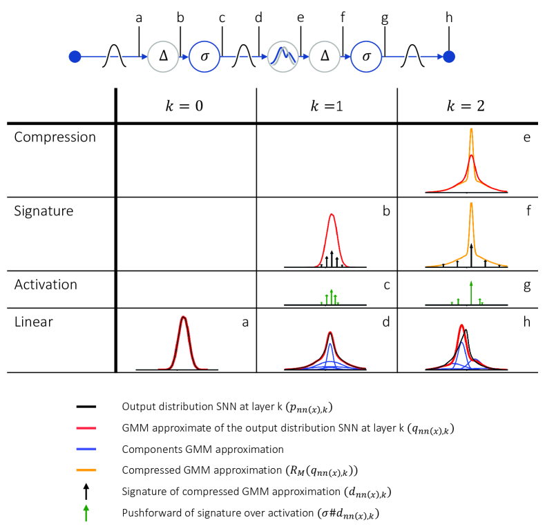
Figure 2: Illustration of the iterative approximation procedure of the output distribution of a single-input single-output SNN with two hidden layers ($K=2$) and one neuron per layer ($n_{1},n_{2}=1$) at a single input point by a Gaussian Mixture distribution.

4.2.1 Approach Outline

Our approach to solving Problem 1 is based on iteratively approximating the output distribution of each layer of a SNN as a mixture of Gaussian distributions and quantifying the approximation error introduced by each operation. As illustrated in Figure 2, following the definition of $p_{nn}({{x}})$ in Eqn (4), the first step is to perform a linear combination of the input point ${{x}}$ with the parameters of the first layer (step a). Because the SNN weights are assumed to be jointly Gaussian and jointly Gaussian random variables are closed under linear combination, this linear operation leads to a Gaussian distribution. Then, before propagating this distribution through an activation function, a signature operation on the resulting distribution is performed; that is, the continuous distribution is approximated into a discrete distribution (step b). After the signature approximation operation, the resulting discrete distribution is passed through the activation function (step c) and a linear combination with the weights of the next layer is performed (step d). Under the assumption that the weights are jointly Gaussian, this linear operation results into a Gaussian mixture distribution of size equal to the support of the discrete distribution resulting from the signature operation. To limit the computational burden of propagating a Gaussian mixture with a large number of components, a compression operation is performed that compresses this distribution into another mixture of Gaussian distributions with at most $M$ components for a given $M$ (step e). After this, a signature operation is performed again on the resulting Gaussian mixture distribution (step f), and the process is repeated until the last layer. Consequently, to construct $q_{nn({{x}})}$, the Gaussian mixture approximation of $p_{nn({{x}})}$, our approach iteratively performs four operations: linear transformation, compression, signature approximation, and propagation through an activation function. To quantify the error in our approach, we derive formal error bounds in terms of the Wasserstein distance for each of these operations and show how the resulting bounds can be combined via interval arithmetic to an upper bound of ${\mathbb{W}}_{2}(p_{nn({{x}})},q_{nn({{x}})})$.

In what follows, first, as it is one of the key elements of our approach, in Section 5 we introduce the concept of signature of a probability distribution and derive error bounds on the 2-Wasserstein distance between a Gaussian mixture distribution and its signature approximation. Then, in Section 6 we formalize the approach described in Figure 2 to approximate a SNN with a GMM and derive bounds for the resulting approximation error. Furthermore, in Subsection 6.4 we prove that $q_{nn(x)}$, the Gaussian mixture approximation resulting from our approach, converges uniformly to $p_{nn(x)},$ the distribution of the SNN, that is, at the cost of increasing the support of the discrete approximating distributions and the number of components of $q_{nn(x)}$, the 1- and 2-Wasserstein distance between $q_{nn(x)}$ and $p_{nn(x)}$ can be made arbitrarily small. Then, in Section 7 we present a detailed algorithm of our approach. Finally, we conclude our paper with Section 8, where an empirical analysis illustrating the efficacy of our approach is performed.

5 Approximating Gaussian Mixture Distributions by Discrete Distributions

One of the key steps of our approach is to perform a signature operation on a Gaussian Mixture distribution, that is, a Gaussian Mixture distribution is approximated with a discrete distribution, called a signature (step b and f in Figure 2). In Subsection 5.1 we formally introduce the notion of the signature of a probability distribution. Then, in Subsection 5.2 we show how for a Gaussian Mixture distribution a signature can be efficiently computed with guarantees on the closeness of the signature and the original Gaussian mixture distribution in the ${\mathbb{W}}_{2}$-distance.

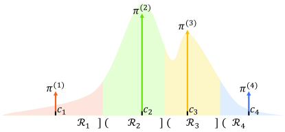
Figure 3: Signature of a continuous probability distribution. The signature is defined by locations $\{{{c}}_{i}\}_{i=1}^{4}$ which imply Voronoi partition $\{{\mathcal{R}}_{i}\}_{i=1}^{4}$. The continuous distribution is discretized w.r.t. the partition by storing all the probability mass ${{{\pi}}^{(i)}}$ covered by ${\mathcal{R}}_{i}$ at ${{c}}_{i}$.

5.1 Signatures: the Discretization of a Continuous Distribution

For a set of points ${\mathcal{C}}=\{{{c}}_{i}\}_{i=1}^{N}\subset{\mathbb{R}}^{d}$ called locations, we define ${\Delta}_{\mathcal{C}}:{\mathbb{R}}^{d}\rightarrow{\mathcal{C}}$ as the function that assigns any ${{z}}\in{\mathbb{R}}^{d}$ to the closest point in ${\mathcal{C}}$, i.e.,

$${\Delta}_{\mathcal{C}}({{z}})=\underset{{{c}}\in{\mathcal{C}}}{\mathrm{argmin}}\|{{z}}-{{c}}\|.$$

The push-forward operation induced by ${\Delta}_{\mathcal{C}}$ is a mapping from ${\mathcal{P}}({\mathbb{R}}^{d})$ to ${\mathcal{D}}_{N}({\mathbb{R}}^{d})$ and defines the signature of a probability distribution. That is, as formalized in Definition 6 below, a signature induced by ${\Delta}_{\mathcal{C}}$ is an approximation of a continuous distribution with a discrete one of support with a cardinality $N$.

Definition 6 (Signature of a Probability Distribution)

The signature of a probability distribution $p\in{\mathcal{P}}({\mathbb{R}}^{d})$ w.r.t. points ${\mathcal{C}}=\{{{c}}_{i}\}_{i=1}^{N}\subset{\mathbb{R}}^{d}$ is the discrete distribution ${\Delta}_{\mathcal{C}}\#p=\sum_{i=1}^{N}\pi^{(i)}\delta_{c_{i}}\in{\mathcal{D}}_{N}({\mathbb{R}}^{d})$, where $\pi^{(i)}=\mathbb{P}_{{{z}}\sim p}[{{z}}\in{\mathcal{R}}_{i}]$ with

$${\mathcal{R}}_{i}=\{{{z}}\in{\mathbb{R}}^{d}:\|{{z}}-{{c}}_{i}\|\leq\|{{z}}-{{c}}_{j}\|,\forall j\in\mathbb{N}_{N},j\neq i\}.$$ (6)

The intuition behind a signature is illustrated in Figure 3: the signature of distribution $p$ is a discretization of $p$ that assigns to each location ${{c}}_{i}\in{\mathcal{C}}$ a probability given by the probability mass of ${\mathcal{R}}_{i}$ according to $p$. Note that partition $\{{\mathcal{R}}_{i}\}_{i=1}^{N}$, as defined in Eqn (6), is the Voronoi partition of ${\mathbb{R}}^{d}$ w.r.t. the Euclidean distance. Hence, the signature of a probability distribution can be interpreted as a discretization of the probability distribution w.r.t. a Voronoi partition of its support. In the remainder, we refer to ${\mathcal{C}}$ as the locations of the signature, $|{\mathcal{C}}|$ as the signature size, $\{{\mathcal{R}}_{i}\}_{i=1}^{N}$ as the partition of a signature, and we call ${\Delta}$ the signature operation. In the next subsection we show how we can efficiently bound $W_{2}(p,{\Delta}_{\mathcal{C}}\#p)$ in the case where $p$ is a Gaussian mixture distribution.

Remark 7

The approximation of a continuous distribution by a discrete distribution, also called a codebook or particle approximation, is a well-known concept in the literature (Graf and Luschgy, 2007; Ambrogioni et al., 2018; Pages and Wilbertz, 2012). The notion of the signature of a probability distribution introduced here is unique in that the discrete approximation is fully defined by the Voronoi partition of the support of the continuous distribution, thereby connecting the concept of signatures to semi-discrete optimal transport (Peyré et al., 2019).

5.2 Wasserstein Bounds for the Signature Operation

The computation of $W_{2}(p,{\Delta}_{\mathcal{C}}\#p)$ requires solving a semi-discrete optimal transport problem, where we need to find the optimal transport plan from each point ${{z}}$ to a specific location ${{c}}_{i}\in{\mathcal{C}}$ (Peyré et al., 2019). Luckily, as illustrated in the following proposition, which is a direct consequence of Theorem 1 in (Ambrogioni et al., 2018), for the case of a signature of a probability distribution, the resulting transport problem can be solved exactly.

Proposition 8

For a probability distribution $p\in{\mathcal{P}}_{2}({\mathbb{R}}^{n})$, and signature locations ${\mathcal{C}}=\{{{c}}_{i}\}_{i=1}^{N}\subset{\mathbb{R}}^{n}$, we have that

$${\mathbb{W}}_{2}^{2}(p,{\Delta}_{\mathcal{C}}\#p)=\sum_{i=1}^{N}\underbrace{{{{\pi}}^{(i)}}{\mathbb{E}}_{{{z}}\sim p}[\|{{z}}-{{c}}_{i}\|^{2}\mid{{z}}\in{\mathcal{R}}_{i}]}_{\eqqcolon{\mathbb{W}}_{2\mid{\mathcal{R}}_{i}}^{2}}.$$

According to Proposition 8, transporting the probability mass at each point ${{z}}$ to a discrete location ${{c}}_{i}$ based on the Voronoi partition of ${\mathbb{R}}^{d}$ guarantees that the cost $\|{{z}}-{{c}}_{i}\|$ is the smallest and leads to the smallest possible transportation cost, i.e., the optimal transportation strategy for the Wasserstein Distance. Proposition 8 is general and guarantees that for any distribution $p\in{\mathcal{P}}_{2}({\mathbb{R}}^{n})$, ${\mathbb{W}}_{2}(p,{\Delta}_{\mathcal{C}}\#p)$ only depends on ${\mathbb{W}}_{2\mid{\mathcal{R}}_{i}}$, the partial $2-$moment of $p$ w.r.t. regions ${\mathcal{R}}_{i}\in\{{\mathcal{R}}_{1},...,{\mathcal{R}}_{N}\}$. In the following proposition, we show how closed-form expressions for ${\mathbb{W}}_{2\mid{\mathcal{R}}_{i}}^{2}$ can be derived for univariate Gaussian distributions. This result is then generalized in Corollary 10 to general multivariate Gaussian distributions.

Proposition 9

For $p=\mathcal{N}(0,1)$, signature locations ${\mathcal{C}}=\{c_{i}\}_{i=1}^{N}\subset{\mathbb{R}}$ and associated partition $\{{\mathcal{R}}_{i}\}_{i=1}^{n}$ with ${\mathcal{R}}_{i}=[l_{i},v_{i}]\subseteq{\mathbb{R}}\cup\{-\infty,\infty\}$ for each $i$, it holds that

$${\mathbb{W}}_{2}^{2}({\Delta}_{{\mathcal{C}}}\#\mathcal{N}(0,1),\mathcal{N}(0,1))=\sum_{i=1}^{N}\nu_{i}+(\mu_{i}-c_{i})^{2},$$ (7)

with,

$$\mu_{i} =\phi(l_{i})-\phi(u_{i}),$$ (8)

$$\nu_{i} =1+l_{i}\phi(l_{i})-u_{i}\phi(u_{i})-[\phi(l_{i})-\phi(u_{i})]^{2}$$ (9)

where $\phi$ is the pdf of a standard (univariate) Gaussian distribution, i.e., $\phi(x)=\frac{1}{\sqrt{2\pi}}\exp(-\frac{x^{2}}{2})$.

In Proposition 9, $\mu_{i}$ and $\nu_{i}$ are the mean and variance of a standard univariate Gaussian distribution restricted on $[l_{i},u_{i}]$. Note that some of the regions in the partition will be unbounded. However, as the standard Gaussian distribution exponentially decays to zero for large $x$, i.e., $\lim_{x\rightarrow\infty}\exp(x^{2})\mathcal{N}(x\mid 0,1)=0$, it follows that the bound in Eqn. (7) is finite even if some of the regions in $\{{\mathcal{R}}_{i}\}_{i=1}^{N}$ are necessarily unbounded.

A corollary of Proposition 9 is Corollary 10, where we extend Proposition 9 to general multivariate Gaussian distributions under the assumption that locations ${\mathcal{C}}$ are such that sets $\{{\mathcal{R}}_{i}\}_{i=1}^{N}$ define a grid in the transformed space induced by the basis of the covariance matrix that we denote as ${{T}}$. As illustrated in Figure 4, it is always possible to satisfy this assumption by taking ${\mathcal{C}}$ as the image of an axis-aligned grid of points under transformation ${{T}}^{-1}$, where ${{T}}^{-1}$ can be computed via an eigendecomposition (Kasim, 2020) or Cholesky decomposition (Davis et al., 2016) of the covariance matrix.

Corollary 10 (of Proposition 9)

For $\mathcal{N}({m},\Sigma)\in\mathcal{G}({\mathbb{R}}^{n})$, let matrix ${{T}}\in{\mathbb{R}}^{n\times n}$ be such that ${{T}}=\mathrm{diag}({{\lambda}})^{-\frac{1}{2}}{{V}}^{T}$ where $\mathrm{diag}({{\lambda}})={{V}}^{T}\Sigma{{V}}$ is a diagonal matrix whose entries are the eigenvalues of $\Sigma$, and ${{V}}$ is the corresponding orthogonal (eigenvector) matrix. Further, let ${\mathcal{C}}=\{{{c}}_{i}\}_{i=1}^{N}\subset{\mathbb{R}}^{n}$ be a set of signature locations on a grid in the transformed space induced by ${{T}}$, i.e.,

$$\mathrm{Post}({\mathcal{C}},{{T}})-\{{m}\}=\bar{{\mathcal{C}}}^{1}\times\bar{{\mathcal{C}}}^{2}\times\ldots\times\bar{{\mathcal{C}}}^{n}$$ (10)

with $\bar{{\mathcal{C}}}^{j}=\{{{T}}^{(j,:)}({\mathcal{C}}-{m})\}\subset{\mathbb{R}}$ the set of signature locations in the transformed space for dimension $j$. Then, it holds that

$${\mathbb{W}}^{2}_{2}({\Delta}_{\mathcal{C}}\#\mathcal{N}({m},\Sigma),\mathcal{N}({m},\Sigma))=\sum_{j=1}^{n}{{{\lambda}}^{(j)}}{\mathbb{W}}^{2}_{2}({\Delta}_{\bar{{\mathcal{C}}}^{j}}\#\mathcal{N}(0,1),\mathcal{N}(0,1)).$$ (11)

Remark 11

For a multivariate Gaussian $p=\mathcal{N}({m},\Sigma)$, the set ${\mathcal{C}}$ of $N>1$ signature locations that minimize ${\mathbb{W}}_{2}({\Delta}_{\mathcal{C}}\#p,p)$ is generally non-unique, and finding any such set is computationally intractable (Graf and Luschgy, 2007). However, for univariate Gaussians, an optimal signature placement strategy exists as outlined in Pagès and Printems (2003) and will be used in Subsection 7.1 to construct grid-constrained signature locations ${\mathcal{C}}$ for multivariate Gaussians.

In the case of Gaussian mixture distributions, i.e., where $p=\sum_{i=1}^{M}{\bar{\pi}^{{(i)}}}\mathcal{N}(m_{i},\Sigma_{i})$, we can simply apply a signature operation to each of the Gaussian distributions in the mixture. In particular, if we call ${\mathcal{C}}=\{{\mathcal{C}}_{1},\ldots,{\mathcal{C}}_{M}\}$ the resulting sets of locations, where ${\mathcal{C}}_{i}$ are the signature locations corresponding to $\mathcal{N}(m_{i},\Sigma_{i})$, then we have that

$${\mathbb{W}}^{2}_{2}\left(\sum_{i=1}^{M}\bar{\pi}^{i}\mathcal{N}(m_{i},\Sigma_{i}),\sum_{i=1}^{M}{\bar{\pi}^{{(i)}}}{\Delta}_{{{\mathcal{C}}}_{i}}\#\mathcal{N}(m_{i},\Sigma_{i})\right)\leq\sum_{i=1}^{M}{\bar{\pi}^{{(i)}}}{\mathbb{W}}^{2}_{2}\left(\mathcal{N}(m_{i},\Sigma_{i}),{\Delta}_{{{\mathcal{C}}}_{i}}\#\mathcal{N}(m_{i},\Sigma_{i})\right).$$ (12)

That is, for a mixture of Gaussian distributions, the resulting 2-Wasserstein distance from a signature can be bounded by a weighted sum of the 2-Wasserstein distance between each of the Gaussian distributions in the mixture and their signatures. In what follows, with an abuse of notation, for a Gaussian mixture distribution $p=\sum_{i=1}^{M}{\bar{\pi}^{{(i)}}}\mathcal{N}(m_{i},\Sigma_{i})$ we will refer to its signature as ${\Delta}_{\mathcal{C}}\#p:=\sum_{i=1}^{M}{\bar{\pi}^{{(i)}}}{\Delta}_{{{\mathcal{C}}}_{i}}\#\mathcal{N}(m_{i},\Sigma_{i})$.

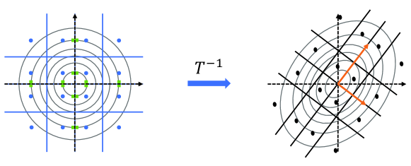
Figure 4: Construction of the signature of a 2D Gaussian distribution (black dots) using the signature of a standard Gaussian distribution (blue dots) as a template. In the space induced by ${{T}}$, that is, the basis of the covariance matrix (orange arrows) of the Gaussian distribution, all dimensions of the Gaussian distribution are independent. Hence, we can take the cross-product of the signatures of each univariate Gaussian marginal in dimension $j$ of the transformed space with signature locations $\bar{{\mathcal{C}}}^{j}$ (green stripes) as a template. The signature in the original space is then obtained by taking the post image of the template under ${{T}}^{-1}$. The blue and black lines represent the edges of the Voronoi partition associated with the signature locations in the transformed and original space, respectively.

6 Stochastic Neural Networks as Gaussian Mixture Models

In this section, we detail and formalize our approach as illustrated in Figure 2 to iteratively approximate a SNN with a GMM. We first consider the case where ${\mathcal{X}}=\{{{x}}\}$, i.e., we approximate the distribution of a SNN over a single input point. The extension of our results for a finite set of input points will be considered in Section 6.3. Last, in Section 6.4, we prove that $q_{nn({\mathcal{X}})}$, i.e., the Gaussian mixture approximation resulting from our approach, converges uniformly to $p_{nn({\mathcal{X}})}$. That is, the error between $p_{nn({\mathcal{X}})}$ and $q_{nn({\mathcal{X}})}$ can be made arbitrarily small by increasing the number of signature points and GMM components.

6.1 Gaussian Mixture Model Approximation of a Neural Network

As shown in Eqn. (4), $p_{nn({{x}})}$, the output distribution of a SNN at input point ${{x}}$, can be represented as a composition of $K$ stochastic operations, one for each layer. To find a Gaussian mixture distribution $q_{nn({{x}})}$ that approximates $p_{nn({{x}})}$, our approach is based on iteratively approximating each of these operations with a GMM, as illustrated in Figure 2. Our approach can then be formalized as in Eqn (13) below for $k\in\{1,\ldots,K\}$:

$$q_{nn(x),1} ={\mathbb{E}}_{{{{z}}}_{0}\sim\delta_{{x}}}[p_{L_{{{w}}_{0}}({{{z}}}_{0})}]$$ (Initialization and Linear operation) (13a)

$$d_{nn(x),k} ={\Delta}_{{\mathcal{C}}_{k}}\#{R}_{M}(q_{nn({{x}}),k})$$ (Compression and Signature operations) (13b)

$$q_{nn(x),k+1} ={\mathbb{E}}_{{{{z}}}_{k}\sim d_{nn({{x}}),k}}[p_{L_{{{w}}_{k}}({\sigma}({{{z}}}_{k}))}]$$ (Activation and Linear operations) (13c)

$$=\sum_{i=1}^{|{\mathcal{C}}_{k}|}{\bar{{{\pi}}}^{{(i)}}}\mathcal{N}\big{(}\bar{{{C}}}_{i}{m}_{W_{k}}+{m}_{b_{k}},\bar{{{C}}}_{i}\Sigma_{W_{k}}\bar{{{C}}}_{i}^{T}+\Sigma_{b_{k}}\big{)}$$

$$q_{nn({{x}})} =q_{nn({{x}}),K+1}$$ (Output) (13d)

where ${\mathcal{C}}_{k}\subset{\mathbb{R}}^{n_{k}}$ is the set of signature locations for layer $k$, $\bar{{{C}}}_{i}={{I}}_{n_{k+1}}\otimes{\sigma}({{c}}_{i}^{T})$ with ${{c}}_{i}\in{\mathcal{C}}_{k}$, and ${m}_{W_{k}},\Sigma_{W_{k}},{m}_{b_{k}},$ and $\Sigma_{b_{k}}$ are the means and the covariances of the weight matrix $W_{k}$ and bias vector $b_{k}$. ${R}_{M}:\mathcal{G}_{\infty}({\mathbb{R}}^{n_{k}})\rightarrow\mathcal{G}_{M}({\mathbb{R}}^{n_{k}})$ is the compression operation that compresses the Gaussian mixture distribution $q_{nn({{x}}),k}$ into a Gaussian Mixture distribution with at most $M$ components, thus limiting the complexity of the approximation. Details on how we perform operation $R_{M}$ using moment matching will be given in Section 7.1. For the rest of this section, ${R}_{M}(q_{nn({{x}}),k})$ can be simply considered as a mapping from the GMM $q_{nn({{x}}),k}$ into a GMM with a maximum size of $M$.

Eqn. (13) consists of the following steps: $q_{nn(x),1}$ is the distribution resulting from a linear combination of the input $x$ with the weights at the first layer, $d_{nn(x),k}$ is the result of a compression and signature operation of $q_{nn({{x}}),k}$, the output of the previous layer. The approximate output distribution $q_{nn(x),k+1}$ at each layer $k$ is obtained by marginalizing $p_{L_{{{w}}_{k}}({\sigma}({{{z}}}_{k}))}$ w.r.t. $d_{nn(x),k}$. We recall that for any fixed ${{{z}}}_{k}$, $p_{L_{{{w}}_{k}}({\sigma}({{{z}}}_{k}))}$ is Gaussian, as it is the distribution of a linear combination of vector ${\sigma}({{{z}}}_{k})$ with matrix $W_{k}$ and vector $b_{k}$, whose components are jointly Gaussian (and Gaussian distributions are closed w.r.t. linear combination). Consequently, as for all $k$, $d_{nn(x),k}$ is a discrete distribution, $q_{nn(x),k+1}$ is a Gaussian mixture distribution with a size equal to the support of $d_{nn(x),k}$.

Remark 12

The approach described in Eqn (13) leads to a Gaussian mixture distribution $q_{nn({{x}})}$ under the assumption that the weight distribution $p_{{{w}}}$ is Gaussian. In the more general case, where $p_{{{w}}}$ is non-Gaussian, one can always recursively approximate $p_{L_{{{w}}_{k}}({{z}})}$ for each $k$ by a discrete distribution using the signature operation. That is, $p_{L_{{{w}}_{k}}({{z}})}$ in Eqn. (13c) is replaced with $q_{L_{{{w}}_{k}}({{z}})}=L_{{{w}}_{k}}({{z}})\#{\Delta}_{{\mathcal{C}}_{{{w}}_{k}}}\#p_{{{w}}_{k}}$, where ${\mathcal{C}}_{{{w}}_{k}}\subset{\mathbb{R}}^{(n_{k+1}+1)\times(n_{k}+1)}$ is the set of signature locations. Applying this additional operation, Eqn (13) will lead to a discrete distribution for $q_{nn({{x}})}$.

6.2 Wasserstein Distance Guarantees

Since $q_{nn(x)}$ is built as a composition of $K$ iterations of the stochastic operations in Eqn (13), to bound ${\mathbb{W}}_{2}(p_{nn(x)},q_{nn(x)})$ we need to quantify the error introduced by each of the steps in Eqn (13). A summary of how each of the operations occurring in Eqn (13) modifies the Wasserstein distance between two distributions is provided in Table 11 (details are given in Appendix A.3). These bounds are composed using interval arithmetic to bound ${\mathbb{W}}_{2}(p_{nn(x)},q_{nn(x)})$ in the following theorem.

Theorem 13

Let $p_{nn({{x}})}$ be the output distribution of a SNN with $K$ hidden layers for input ${{x}}\in{\mathbb{R}}^{n_{0}}$ and $q_{nn({{x}})}$ be a Gaussian mixture distribution built according to Eqn. (13). For $k\in\{1,\ldots,K\}$ iteratively define $\hat{{\mathbb{W}}}_{2}$ as

$$\hat{{\mathbb{W}}}_{2,1}=0,$$ (14a)

$$\hat{{\mathbb{W}}}_{2,k+1}=\hat{\mathcal{S}}_{2,{{w}},k}\left[{\mathcal{L}}_{{\sigma}}\hat{{\mathbb{W}}}_{2,k}+{\mathcal{L}}_{{\sigma}}\hat{{\mathbb{W}}}_{2,{R},k}+\hat{{\mathbb{W}}}_{2,{\Delta},k}\right],$$ (14b)

$$\hat{{\mathbb{W}}}_{2}=\hat{{\mathbb{W}}}_{2,K+1},$$ (14c)

where $\hat{\mathcal{S}}_{2,{{w}},k}$, $\hat{{\mathbb{W}}}_{2,{\Delta},k}$ and $\hat{{\mathbb{W}}}_{2,{R},k}$ are such that

$${\mathbb{E}}_{{{{W}}}_{k}\sim p_{w_{k}}}[\|{{{W}}}_{k}\|^{2}]^{\frac{1}{2}} \leq\hat{\mathcal{S}}_{2,{{w}},k},$$ (15)

$${\mathbb{W}}_{2}({\sigma}\#{R}_{M}(q_{nn({{x}}),k}),{\sigma}\#{\Delta}_{{\mathcal{C}}_{k}}\#{R}_{M}(q_{nn({{x}}),k})) \leq\hat{{\mathbb{W}}}_{2,{\Delta},k},$$ (16)

$${\mathbb{W}}_{2}(q_{nn({{x}}),k},{R}_{M}(q_{nn({{x}}),k})) \leq\hat{{\mathbb{W}}}_{2,{R},k}.$$ (17)

Then, it holds that

$${\mathbb{W}}_{2}(p_{nn(x)},q_{nn(x)})\leq\hat{{\mathbb{W}}}_{2}(p_{nn(x)},q_{nn(x)})\coloneqq\hat{{\mathbb{W}}}_{2}.$$ (18)

The proof of Theorem 13 is reported in Appendix A.3 and is based on the triangular inequality property of the 2-Wasserstein distance, which allows us to bound ${\mathbb{W}}_{2}(p_{nn({{x}})},q_{nn({{x}})})$ iteratively over the hidden layers. Note that Theorem 13 depends on quantities $\hat{\mathcal{S}}_{2,{{w}},k}$, $\hat{{\mathbb{W}}}_{2,{\Delta},k}$ and $\hat{{\mathbb{W}}}_{2,{R},k}$, which can be computed as follows. First, $\hat{\mathcal{S}}_{2,{{w}},k}$ is a bound on the expected spectral norm of the weight matrices of the $k$-th layer, which can be obtained according to the following Lemma.

Lemma 14

For distribution $p_{{W}}\in{\mathcal{P}}({\mathbb{R}}^{n\times m})$, we have that

$${\mathbb{E}}_{{{W}}\sim p_{{W}}}[\|{{W}}\|^{2}]^{\frac{1}{2}} \leq\Big{(}\sum_{i,j}{\mathbb{E}}_{\bar{{{W}}}\sim\tau_{{M}}\#p_{{W}}}[({\bar{{{W}}}^{{(i,j)}}})^{2}]\Big{)}^{\frac{1}{2}}+\|{{M}}\|$$ (19)

where $\tau_{{M}}:{\mathbb{R}}^{n\times m}\rightarrow{\mathbb{R}}^{n\times m}$ is a translation defined by $\tau_{{M}}({{W}})={{W}}+{{M}}$ and ${{M}}={\mathbb{E}}_{{{W}}\sim p_{{W}}}[{{W}}]$, i.e., $\tau_{{M}}\#p_{{W}}$ is a zero mean distribution.

The proof of Lemma 14 relies on the Minkowski inequality and the fact that the spectral norm is upper bounded by the Frobenius norm, as explained in Appendix A.3. Furthermore, $\hat{{\mathbb{W}}}_{2,{\Delta},k}$ can be computed as in Eqn. (12) using Corollaries 10 and 27. Lastly, $\hat{{\mathbb{W}}}_{2,{R},k}$ bounds the distance between Gaussian mixture distributions, which can be efficiently bounded using the ${\mathbb{MW}}_{2}$ distance introduced in Delon and Desolneux (2020) and formally defined below.

Definition 15 (${\mathbb{MW}}_{2}$ Distance)

Let $p=\sum_{i=1}^{N_{p}}{{{\pi}}_{p}^{{(i)}}}p_{i}\in\mathcal{G}_{N_{1}}({\mathbb{R}}^{n})$ and $q=\sum_{j=1}^{N_{q}}{{{\pi}}_{q}^{{(j)}}}q_{j}\in\mathcal{G}_{N_{1}}({\mathbb{R}}^{n})$ be two Gaussian Mixture distributions. The ${\mathbb{MW}}_{2}$-distance is defined as

$${\mathbb{MW}}_{2}(p,q)\coloneqq\left(\inf_{\gamma\in\Gamma(p,q)\cap\mathcal{G}_{<\infty}({\mathbb{R}}^{n}\times{\mathbb{R}}^{n})}{\mathbb{E}}_{({{x}},{{z}})\sim\gamma}[\|{{x}}-{{z}}\|^{2}]\right)^{\frac{1}{2}}=\bigg{(}\min_{{{\pi}}\in\Gamma({{\pi}}_{p},{{\pi}}_{q})}\sum_{i}^{N_{p}}\sum_{j}^{N_{q}}{{{\pi}}^{{(i,j)}}}{\mathbb{W}}_{2}^{2}(p_{i},q_{j})\bigg{)}^{\frac{1}{2}}.$$ (20)

The ${\mathbb{MW}}_{2}$ distance is a Wasserstein-type distance that restricts the set of possible couplings to Gaussian mixtures. Consequently, it can be formulated as a finite discrete linear program with $N_{p}\cdot N_{q}$ optimization variables and coefficients being the Wasserstein distance between the mixture’s Gaussian components, which have closed-form expressions (Givens and Shortt, 1984).

Operation	Wasserstein Bounds		Ref.
Linear
	${\mathbb{W}}_{2}({\mathbb{E}}_{{{x}}\sim p}[p_{L_{{{w}}}({{x}})}],{\mathbb{E}}_{{{z}}\sim q}[p_{L_{{{w}}}({{z}})}])$	$\leq{\mathbb{E}}_{({{W}},{{b}})\sim p_{w}}[\|{{W}}\|^{2}]^{\frac{1}{2}}{\mathbb{W}}_{2}(p,q)$	Prop. 25
Activation
	${\mathbb{W}}^{2}_{2}({\sigma}\#p,{\sigma}\#{\Delta}_{\mathcal{C}}\#p)$	$\leq\sum_{i=1}^{|{\mathcal{C}}|}{\mathcal{L}}^{2}_{{\sigma}\mid{\mathcal{R}}_{i}}{\mathbb{W}}_{2\mid{\mathcal{R}}_{i}}^{2}$	Corol. 27
	${\mathbb{W}}_{2}({\sigma}\#p,{\sigma}\#q)$	$\leq{\mathcal{L}}_{{\sigma}}{\mathbb{W}}_{2}(p,q)$
Signature/ Compression	$h\in\{{\Delta}_{\mathcal{C}},{R}_{R}\}$
	${\mathbb{W}}_{2}(p,h\#q)$	$\leq{\mathbb{W}}_{2}(p,q))+{\mathbb{W}}_{2}(q,h\#q)$	Prop. 28

Table 1: Summary of the bounds on the Wasserstein distance between a distribution $p\in{\mathcal{P}}_{2}({\mathbb{R}}^{n})$ and $q\in{\mathcal{P}}_{2}({\mathbb{R}}^{n})$ obtained by pushing forward $p$ through the most common SNN operation types. Here, ${\mathcal{L}}_{\sigma}$ and ${\mathcal{L}}_{\sigma\mid{\mathcal{R}}_{i}}$ are, respectively, the global Lipschitz constant and the local Lipschitz constant in region ${\mathcal{R}}_{i}$ of the piecewise continuous activation function $\sigma$, while ${\mathbb{W}}_{2\mid{\mathcal{R}}_{i}}^{2}$ is as defined in Proposition 8. The propositions and their proofs are provided in Appendix A.3.

6.3 Approximation for Sets of Input Points

We now consider the case where ${\mathcal{X}}=\{{{x}}_{1},...,{{x}}_{D}\}$, that is, a finite set of input points, and extend our approach to compute a Gaussian mixture approximation of $p_{nn({\mathcal{X}})}$. We first note that $p_{nn({\mathcal{X}})}$ can be equivalently represented by extending Eqn. (4) as follows, where in the equation below ${\mathrm{vec}}({\mathcal{X}})=({{x}}_{1}^{T},\ldots,{{x}}_{D}^{T})^{T}$ is the vectorization of ${\mathcal{X}}$

$$p_{nn({\mathcal{X}}),1}={\mathbb{E}}_{{{z}}_{0}\sim\delta_{{\mathrm{vec}}({\mathcal{X}})}}[p_{L_{{{w}}_{0}}^{D}({{z}}_{0})}],$$ (21)

$$p_{nn({\mathcal{X}}),k+1}={\mathbb{E}}_{{{z}}_{k}\sim p_{nn({\mathcal{X}}),k}}[p_{L^{D}_{{{w}}_{k}}({\sigma}({{z}}_{k}))}],\qquad k\in\{1,...,K\},$$

$$p_{nn({\mathcal{X}})}=p_{nn({\mathcal{X}}),K+1},$$

where $L_{{{w}}_{k}}^{D}:{\mathbb{R}}^{D\cdot n_{k}}\rightarrow{\mathbb{R}}^{D\cdot n_{k}}$ is the stacking of $D$ times $L_{k}$, i.e., $L_{{{w}}_{k}}^{D}(({{z}}_{1}^{T},\ldots,{{z}}_{D}^{T})^{T})=(L_{{{w}}_{k}}({{z}}_{1})^{T},\ldots,\newline L_{{{w}}_{k}}({{z}}_{D})^{T})^{T}$, and $p_{L^{D}_{{{w}}}({{z}})}=L^{D}_{{{w}}_{k}}({{z}})\#p_{{{w}}_{k}}$. That is, $p_{nn({\mathcal{X}})}$ is computed by stacking $D$ times the neural network for the inputs in ${\mathcal{X}}$. Following the same steps as in the previous section, $p_{nn({\mathcal{X}})}$ can then be approximated by the Gaussian Mixture distribution $q_{nn({\mathcal{X}})}$, for $k\in\{1,\ldots,K\}$ defined as

$$q_{nn({\mathcal{X}}),1} ={\mathbb{E}}_{{{{z}}}_{0}\sim\delta_{{\mathrm{vec}}({\mathcal{X}})}}[p_{L^{D}_{{{w}}_{0}}({{{z}}}_{0})}]$$ (Initialization and Linear operation) (22a)

$$d_{nn({\mathcal{X}}),k} ={\Delta}_{{\mathcal{C}}_{k}}\#{R}_{M}(q_{nn({\mathcal{X}}),k})$$ (Compression and Signature operations) (22b)

$$q_{nn({\mathcal{X}}),k+1} ={\mathbb{E}}_{{{{z}}}_{k}\sim d_{nn({\mathcal{X}}),k}}[p_{L^{D}_{{{w}}_{k}}({\sigma}({{{z}}}_{k}))}]$$ (Activation and Linear operations) (22c)

$$q_{nn({\mathcal{X}})} =q_{nn({\mathcal{X}}),K+1}$$ (Output) (22d)

where ${\mathcal{C}}_{k}\subset{\mathbb{R}}^{D\cdot n_{k}}$ are the signature locations at layer $k$, and $M\in\mathbb{N}$ is the size of compressed mixtures. A corollary of Theorem 13 is the following proposition that bounds the approximation error of $q_{nn({\mathcal{X}})}$.

Proposition 16

Let $p_{nn({\mathcal{X}})}$ be the joint distribution of a SNN with $K$ hidden layers over a finite set of input points ${\mathcal{X}}=\{{{x}}_{i}\}_{i=1}^{D}\subset{\mathbb{R}}^{n_{0}}$ and $q_{nn({\mathcal{X}})}$ be a Gaussian mixture distribution built according to Eqn. (22). For $k\in\{1,\ldots,K\}$ iteratively define $\hat{{\mathbb{W}}}_{2}$ as in Eqn. (14) with $\hat{\mathcal{S}}_{2,{{w}},k}$, $\hat{{\mathbb{W}}}_{2,{\Delta},k}$ and $\hat{{\mathbb{W}}}_{2,{R},k}$ such that

$$D^{\frac{1}{2}}{\mathbb{E}}_{{{{W}}}_{k}\sim p_{w_{k}}}[\|{{{W}}}_{k}\|^{2}]^{\frac{1}{2}} \leq\hat{\mathcal{S}}_{2,{{w}},k},$$ (23)

$${\mathbb{W}}_{2}({\sigma}\#{R}_{M}(q_{nn({\mathcal{X}}),k}),{\sigma}\#{\Delta}_{{\mathcal{C}}_{k}}\#{R}_{M}(q_{nn({\mathcal{X}}),k})) \leq\hat{{\mathbb{W}}}_{2,{\Delta},k},$$ (24)

$${\mathbb{W}}_{2}(q_{nn({\mathcal{X}}),k},{R}_{M}(q_{nn({\mathcal{X}}),k})) \leq\hat{{\mathbb{W}}}_{2,{R},k}.$$ (25)

Then, it holds that

$${\mathbb{W}}_{2}(p_{nn({\mathcal{X}})},q_{nn({\mathcal{X}})})\leq\hat{{\mathbb{W}}}_{2}(p_{nn({\mathcal{X}})},q_{nn({\mathcal{X}})})\coloneqq\hat{{\mathbb{W}}}_{2}.$$

In the above proposition, we can set $\hat{\mathcal{S}}_{2,{{w}},k}$ as in the single-point case, scaled by the square root of the number of input points. Similar to the single point-case, $\hat{{\mathbb{W}}}_{2,{\Delta},k}$ can be computed as in Eqn. (12) using Corollaries 10 and 27, and $\hat{{\mathbb{W}}}_{2,{R},k}$ can be taken as the ${\mathbb{MW}}_{2}$ distance between GMMs $q_{nn({\mathcal{X}}),k}$ and ${R}_{M}(q_{nn({\mathcal{X}}),k})$. Note that the effect of multiple input points on the error introduced by $\hat{{\mathbb{W}}}_{2,{\Delta},k}$ and $\hat{{\mathbb{W}}}_{2,{R},k}$ depends on the specific choice of points in ${\mathcal{X}}$. For points in ${\mathcal{X}}$ where $q_{nn({\mathcal{X}}),k}$ is highly correlated, the error will be similar to that of a single-input case. However, if there is little correlation, the error bound will increase linearly with the number of points.

6.4 Convergence Analysis

In Theorem 13 and Proposition 16 we derived error bounds on the distance between $q_{nn({\mathcal{X}})}$ and $p_{nn({\mathcal{X}})}$. In the following theorem, we prove that if one allows for the size of $q_{nn({{x}})}$ to be arbitrarily large, then the error converges to zero.

Theorem 17

Let $p_{nn({\mathcal{X}})}$ be the output distribution of a SNN with $K$ hidden layers for a finite set of inputs ${\mathcal{X}}\subset{\mathbb{R}}^{n_{0}}$, $q_{nn({\mathcal{X}})}$ be a Gaussian mixture distribution built according to Eqn. (22), and $\hat{{\mathbb{W}}}_{2}$ be the upper bound on ${\mathbb{W}}_{2}(p_{nn({\mathcal{X}})},q_{nn({\mathcal{X}})})$ defined according to Eqn. (14). Then, for any $\epsilon>0$, there exist sets of signature locations ${\mathcal{C}}_{1},\ldots,{\mathcal{C}}_{K}$ of finite sizes, and a compression size $M$, such that $\hat{{\mathbb{W}}}_{2}\leq\epsilon$.

The proof of Theorem 17 is based on iteratively showing that for any $k$, $\hat{{\mathbb{W}}}_{2,k}$ in Eqn. (14b) can be made arbitrarily small. To do that, we extend the results in Graf and Luschgy (2007) and show that for a GMM $q_{nn({\mathcal{X}}),k}$ its 2-Wasserstein distance from the signature approximation ${\Delta}_{\{{\mathcal{C}}_{1},\ldots,{\mathcal{C}}_{|{\mathcal{C}}|}\}}\#q_{nn({\mathcal{X}}),k}$ can be made smaller than any $\bar{\epsilon}>0$ by selecting signature points ${\mathcal{C}}_{i}$ for each element $i$ as center points of a grid partitioning a compact set ${\mathcal{X}}$ so that $\int_{{\mathbb{R}}\setminus{\mathcal{X}}}\|{{z}}\|^{2}dq_{nn({\mathcal{X}}),k}({{z}})\leq\bar{\epsilon}/2$. Note that since for all $k$, $q_{nn({{x}}),k}\in{\mathcal{P}}_{2}(\cdot)$ it is always possible to find a compact ${\mathcal{X}}$ so that the assumption is satisfied. Furthermore, the signature points can always be taken to satisfy Eqn. 10 in Corollary 10, by taking, for each element, the grid to align with the basis of the covariance matrix.

Remark 18

While in the proof of Theorem 17 we use uniform grids for each component of $q_{nn({\mathcal{X}}),k}$, in practice, adaptive, non-uniform gridding can guarantee closeness in ${\mathbb{W}}_{2}$-distance with the same precision for smaller grid sizes.

7 Algorithmic Framework

In this section, the theoretical methodology to solve Problem 1 developed in the previous sections is translated into an algorithmic framework. First, following Eqn. (22), we present an algorithm to construct the Gaussian mixture approximation of a SNN with error bounds in terms of the 2-Wasserstein distance, including details on the compression step. Then, we rely on the fact that the error bound resulting from our approach is piecewise differentiable with respect to the parameters of the SNN to address the complementary problem highlighted in Remark 4. This problem involves deriving an algorithm to optimize the parameters of a SNN such that the SNN approximates a given GMM.

input : $p_{nn({\mathcal{X}})}$

output : $q_{nn({\mathcal{X}})}$; $\hat{{\mathbb{W}}}_{2}(p_{nn({\mathcal{X}})},q_{nn({\mathcal{X}})})$

begin

      1 Initialize $q_{nn({\mathcal{X}}),1}$ as in Eqn. (22a) and $\hat{{\mathbb{W}}}_{2,1}$ as in Eqn. (14a)

       for $k\in\{1,\ldots,K\}$ do

            2 Compress $q_{nn({\mathcal{X}}),k}$ using Algorithm 3 [Eqn. (22b)]

            3 Compute $\hat{{\mathbb{W}}}_{2,{R},k}$ using the ${\mathbb{MW}}_{2}$ distance [Eqn. (25)]

            4 Get signature $d_{nn({\mathcal{X}}),k}$ of ${R}_{M}(q_{nn({\mathcal{X}}),k})$ and $\hat{{\mathbb{W}}}_{2,{\Delta},k}$ via Alg. 2 [Eqns. (22b) & (24)]

            5 Construct $q_{nn({\mathcal{X}}),k+1}$ as in Eqn. (22c)

            6 Compute $\hat{\mathcal{S}}_{2,{{w}},k}$ using Lemma 14 [Eqn. (23)]

            7 Compute $\hat{{\mathbb{W}}}_{2,k+1}$ as in Eqn. (14c)

      8Set $q_{nn({\mathcal{X}})}=q_{nn({\mathcal{X}}),K+1}$ and $\hat{{\mathbb{W}}}_{2}(p_{nn({\mathcal{X}})},q_{nn({\mathcal{X}})})=\hat{{\mathbb{W}}}_{2,K+1}$ [Eqns. (22d) & (14c)]

Algorithm 1 Gaussian Mixture Approximation of a SNN

7.1 Construction of the GMM Approximation of a SNN

The procedure to build a Gaussian mixture approximation $q_{nn({\mathcal{X}})}$ of $p_{nn({\mathcal{X}})}$, i.e. the output distribution of a SNN at a set of input points ${\mathcal{X}}$ as in Eqn (22), is summarized in Algorithm 1. The algorithm consists of a forward pass over the layers of the SNN. First, the Gaussian output distribution after the first linear layer is constructed (line 1). Then, for each layer $k>0$, $q_{nn({\mathcal{X}}),k}$ is compressed to a mixture of size $M$ (line 2); the signature of $R_{M}(q_{nn({\mathcal{X}})})$ is computed (line 4); and the signature is passed through the activation and linear layer to obtain $q_{nn({\mathcal{X}}),k+1}$ (line 5). Parallel to this, following Proposition 16, error bounds on the 2-Wasserstein distance are computed for the compression operation (line 3), signature and activation operation (line 4), and linear operation (line 6), which are then composed into a bound on ${\mathbb{W}}_{2}(p_{nn({\mathcal{X}}),k+1},q_{nn({\mathcal{X}}),k+1})$ that is propagated to the next layer (line 8).

Signature Operation

The signature operation on $q_{nn({\mathcal{X}}),k}$ in line 4 of Algorithm 1 is performed according to the steps in Algorithm 2. That is, the signature of $q_{nn({\mathcal{X}}),k}$ is taken as the mixture of the signatures of the components of $q_{nn({\mathcal{X}}),k}$ (lines 1-7). For each Gaussian component of the mixture, to ensure an analytically exact solution for the Wasserstein distance resulting from the signature, we position its signature locations on a grid that aligns with the covariance matrix’s basis vectors, i.e., the locations satisfy the constraint as in Eqn. (10) of Corollary 10. In particular, the grid of signatures is constructed so that the Wasserstein distance from the signature operation is minimized. According to the following proposition, the problem of finding this optimal grid can be solved in the transformed space, in which the Gaussian is independent over its dimensions.

Proposition 19

For $\mathcal{N}({m},\Sigma)\in{\mathcal{P}}({\mathbb{R}}^{n})$, let matrix ${{T}}\in{\mathbb{R}}^{n\times n}$ be such that ${{T}}=\mathrm{diag}({{\lambda}})^{-\frac{1}{2}}{{V}}^{T}$ where $\mathrm{diag}({{\lambda}})={{V}}^{T}\Sigma{{V}}$ is a diagonal matrix whose entries are the eigenvalues of $\Sigma$, and ${{V}}$ is the corresponding orthogonal (eigenvector) matrix. Then,

$$\underset{\begin{subarray}{c}\{\bar{{\mathcal{C}}}^{1},\ldots,\bar{{\mathcal{C}}}^{n}\}\subset{\mathbb{R}},\\ \sum_{i=1}^{n}|\bar{{\mathcal{C}}}^{j}|=N\end{subarray}}{\mathrm{argmin}}{\mathbb{W}}_{2}({\Delta}_{\mathrm{Post}(\bar{{\mathcal{C}}^{1}}\times\ldots\times\bar{{\mathcal{C}}}^{n},{{T}}^{-1})+\{{m}\}}\#\mathcal{N}({m},\Sigma),\mathcal{N}({m},\Sigma))=\{\bar{{\mathcal{C}}}(N_{1}^{*}),\ldots,\bar{{\mathcal{C}}}(N_{n}^{*})\},$$

where

$$\bar{{\mathcal{C}}}(N) =\underset{{\mathcal{C}}\in{\mathbb{R}},|{\mathcal{C}}|=N}{\mathrm{argmin}}{\mathbb{W}}_{2}({\Delta}_{{\mathcal{C}}}\#\mathcal{N}(0,1),\mathcal{N}(0,1))$$ (26)

$$\{N_{1}^{*},\ldots,N_{n}^{*}\} =\underset{\begin{subarray}{c}\{N_{1},\ldots,N_{n}\}\in\mathbb{N}^{n},\\ \prod_{j=1}^{n},N_{j}=N\end{subarray}}{\mathrm{argmin}}\sum_{j=1}^{n}{{{\lambda}}^{(j)}}{\mathbb{W}}_{2}({\Delta}_{\bar{{\mathcal{C}}}(N_{i})}\#\mathcal{N}(0,1),\mathcal{N}(0,1)).$$ (27)

Following Proposition 19, the optimal grid of signature locations of any Gaussian is defined by the optimal signature locations for a univariate Gaussian (Eqn. (26)) and the optimal size of each dimension of the grid (Eqn. (27)). While the optimization problem in Eqn. (26) is non-convex, it can be solved up to any precision using the fixed-point approach proposed in Kieffer (1982). In particular, we solve the problem once for a range of grid sizes $N$ and store the optimal locations in a lookup table that is called at runtime. To address the optimization problem in Eqn. (27), we use that ${\mathbb{W}}_{2}({\Delta}_{\bar{{\mathcal{C}}}(N)}\#\mathcal{N}(0,1),\mathcal{N}(0,1))$, with optimal locations $\bar{{\mathcal{C}}}(N)$ as in Eqn. (26), is strictly decreasing for increasing $N$ so that even for large $N$, the number of feasible non-dominated candidates $\{N_{1},\ldots,N_{n}\}$ is small.

input : $\sum_{i=1}^{M}{\bar{{{\pi}}}^{{(i)}}}\mathcal{N}({m}_{i},\Sigma_{i})$

output : $d=\sum_{j=1}^{N}{{{\pi}}^{(j)}}\delta_{{{c}}_{j}}$; $\hat{{\mathbb{W}}}_{2,{\Delta}}$

begin

       Construct the signature of the components of the mixture using the (fixed and optimal) signature of $\mathcal{N}(0,1)$ with locations ${\mathcal{C}}_{1d}$:

       for $i\in\{1,\ldots,M\}$ do

            1 Compute eigenvalues vector ${{\lambda}}_{i}$ and eigenvector matrix ${{V}}_{i}$ of $\Sigma_{i}$

            2 Find the optimal grid sizes $\{N_{1}^{*},\ldots,N_{n}^{*}\}$ for ${{\lambda}}_{i}$ according to Eqn. (26)

            3 Take grid $\bar{{\mathcal{C}}}=\bar{{\mathcal{C}}}(N_{1})\times\ldots\times\bar{{\mathcal{C}}}(N_{n})$ , with $\bar{{\mathcal{C}}}(N_{i})$ as in Eqn. (27)

            4 Transform the grid to the original space: ${\mathcal{C}}_{i}=\mathrm{Post}(\bar{{\mathcal{C}}},{{S}})+{m}_{i}$ with ${{S}}={{V}}_{i}\mathrm{diag}({{\lambda}}_{i})^{\frac{1}{2}}$

            5 Define $d_{i}=\sum_{j=1}^{|{\mathcal{C}}_{i}|}{{{\pi}}^{{(j)}}}{{c}}_{j}$ where ${{c}}_{j}\in{\mathcal{C}}_{i}$ and ${{{\pi}}^{{(j)}}}=\mathbb{P}_{{{z}}\sim\mathcal{N}({m}_{i},\Sigma_{i})}[{{z}}\in{\mathcal{R}}_{j}]$

            6 Compute $\hat{{\mathbb{W}}}_{2,{\Delta},i}=\sum_{j=1}^{|{\mathcal{C}}|}{\mathcal{L}}_{{\sigma}\mid{\mathcal{R}}_{j}}{{{\pi}}^{(j)}}\hat{{\mathbb{W}}}_{2\mid{\mathcal{R}}_{i}}$ with $\hat{{\mathbb{W}}}_{2\mid{\mathcal{R}}_{j}}=\sum_{l=1}^{n}{{{\lambda}}_{i}^{{(l)}}}({{{\nu}}_{j}^{{(l)}}}+({{{\mu}}_{j}^{{(l)}}}-{{{c}}_{j}^{{(l)}}}))$ with ${{{\mu}}_{j}^{{(l)}}}$ as in Eqn. (8) and ${{{\nu}}_{j}^{{(l)}}}$ as in Eqn. (9) of Prop. 10

            

      7Set $d=\sum_{i=1}^{M}{\bar{{{\pi}}}^{{(i)}}}d_{i}$ and $\hat{{\mathbb{W}}}_{2,{\Delta}}^{2}=\sum_{i=1}^{M}{\bar{{{\pi}}}^{{(i)}}}{\mathbb{W}}_{2,{\Delta},i}^{2}$

      

Algorithm 2 Signatures of Gaussian Mixtures

Compression Operation

Our approach to compress a GMM of size $N$ into a GMM of size $M<N$, i.e., operation ${R}_{M}$ in Eqn. (13b), is described in Algorithm 3 and is based on the M-means clustering using Lloyd’s algorithm (Lloyd, 1982) on the means of the mixture’s components (line 1). That is, each cluster is substituted by a Gaussian distribution with mean and covariance equal to those of the mixture in the cluster (line 2).

Remark 20

For the compression of discrete distributions, such as in the case of Bayesian inference via dropout, we present a computationally more efficient alternative procedure to Algorithm 3 in Section B of the Appendix. Note that in the dropout case, the support of the multivariate Bernoulli distribution representing the dropout masks at each layer’s input grows exponentially with the layer width, making compression of paramount importance in practice.

input : $\bar{q}=\sum_{i=1}^{\bar{M}}{\bar{{{\pi}}}^{{(i)}}}\mathcal{N}(\bar{{m}}_{i},\bar{\Sigma}_{i})$

output : $q=\sum_{j=1}^{M}{{{\pi}}^{{(j)}}}\mathcal{N}({m}_{j},\Sigma_{j})$

begin

      1 Collect the components of $\bar{q}$ in $M$ clusters by applying $M$-means clustering to $\{\bar{{m}}_{1},\ldots,\bar{{m}}_{\bar{M}}\}$ using Lloyd’s Algorithm

       for $j\in\{1,\ldots,M\}$ do

             Compress all components in the $j$-th cluster with indices in ${\mathcal{I}}_{j}$ to component $\mathcal{N}({m}_{j},\Sigma_{j})$ with weight ${{{\pi}}^{(j)}}$ by taking the weighted average of the means and covariances:

            2 ${{{\pi}}^{(j)}}=\sum_{i\in{\mathcal{I}}_{j}}{\bar{{{\pi}}}^{{(i)}}}$; ${m}_{j}=\frac{1}{{{{\pi}}^{(j)}}}\sum_{i\in{\mathcal{I}}_{j}}{\bar{{{\pi}}}^{{(i)}}}\bar{{m}}_{i}$; $\Sigma_{j}=\frac{1}{{{{\pi}}^{(j)}}}\sum_{i\in{\mathcal{I}}_{j}}{\bar{{{\pi}}}^{{(i)}}}[\bar{\Sigma}_{i}+(\bar{{m}}_{i}-{m}_{j})(\bar{{m}}_{i}-{m}_{j})^{T}]$

            

      

Algorithm 3 Compress Gaussian Mixture

7.2 Construction of a SNN Approximation of a GMM

The algorithmic framework presented in the previous subsection finds the Gaussian Mixture distribution that best approximates the output distribution of a SNN and returns bounds on their distance. In this subsection, we show how our results can be employed to solve the complementary problem of finding the weight distribution of a SNN to best match a given GMM.

Let us consider a finite set of input points ${\mathcal{X}}\subset{\mathbb{R}}^{n_{0}}$ and a SNN and GMM, whose distributions at ${\mathcal{X}}$ are respectively $p_{nn(\mathcal{X})}$ and $q_{gmm({\mathcal{X}})}$. Furthermore, in this subsection, we assume that the weight distribution $p_{{w}}$ of the SNN is parametrized by a set of parameters $\psi$. For instance, in the case where $p_{{w}}$ is a multivariate Gaussian distribution, then $\psi$ parametrizes its mean and covariance. Note that, consequently, also $p_{nn({\mathcal{X}})}$ depends on $\psi$ through Eqn. (21). To make the dependence explicit, in what follows, we will use a superscript to emphasize the dependency on $\psi$. Then, our goal is to find $\psi^{*}=\mathrm{argmin}_{\psi}{\mathbb{W}}_{2}(p_{nn(\mathcal{X})}^{\psi},q_{gmm(\mathcal{X})})$. To do so, we rely on Corollary 21 below, which uses the triangle inequality to extend Proposition 16.

Corollary 21 (of Proposition 16)

Let ${\mathcal{X}}\subset{\mathbb{R}}^{n_{0}}$ be a finite set of input points. Then, for a SNN and a GMM, whose distributions at ${\mathcal{X}}$ are respectively $p_{nn(\mathcal{X})}^{\psi}$ and $q_{gmm({\mathcal{X}})},$ it holds that

$${\mathbb{W}}_{2}(p_{nn({\mathcal{X}})}^{\psi},q_{gmm({\mathcal{X}})})\leq\hat{{\mathbb{W}}}_{2}(p_{nn({\mathcal{X}})}^{\psi},q_{nn({\mathcal{X}})}^{\psi})+{\mathbb{MW}}_{2}(q_{nn({\mathcal{X}})}^{\psi},q_{gmm({\mathcal{X}})}),$$ (28)

where the GMM $q_{nn({\mathcal{X}})}^{\psi}$ and the bound $\hat{{\mathbb{W}}}_{2}$ are obtained via Algorithm 1, and ${\mathbb{MW}}_{2}$ is as defined in Definition 15, with $q_{nn({\mathcal{X}})}^{\psi}$ also depending on $\psi$ through Eqn. (22).

Using, Corollary 21, we can approximate $\psi^{*}$ as follows

$$\psi^{*}\approx\underset{\psi}{\mathrm{argmin}}\left\{\beta\hat{{\mathbb{W}}}_{2}(p^{\psi}_{nn({\mathcal{X}})},q^{\psi}_{nn({\mathcal{X}})})+(1-\beta){\mathbb{MW}}_{2}(q^{\psi}_{nn({\mathcal{X}})},q_{gmm({\mathcal{X}})})\right\},$$ (29)

where $\beta\in[0,1]$ allows us to trade off between the gap between the bound $\hat{{\mathbb{W}}}_{2}(p^{\psi}_{nn({\mathcal{X}})},q^{\psi}_{nn({\mathcal{X}})})$ and ${\mathbb{W}}_{2}(p^{\psi}_{nn({\mathcal{X}})},q^{\psi}_{nn({\mathcal{X}})})$ and the gap between the bound ${\mathbb{MW}}_{2}(q^{\psi}_{nn({\mathcal{X}})},q_{gmm({\mathcal{X}})})$ and ${\mathbb{W}}_{2}(q^{\psi}_{nn({\mathcal{X}})},q_{gmm({\mathcal{X}})})$. For instance, in the case where $q^{\psi}_{nn({\mathcal{X}})}$ and $q_{gmm({\mathcal{X}})}$ are Gaussian distributions, ${\mathbb{MW}}_{2}(q^{\psi}_{nn({\mathcal{X}})},q_{gmm({\mathcal{X}})})$ equals ${\mathbb{W}}_{2}(q^{\psi}_{nn({\mathcal{X}})},q_{gmm({\mathcal{X}})})$, leading us to choose $\beta<\frac{1}{2}$. As discussed next, under the assumption that the mean and covariance of $p_{{w}}$ are differentiable with respect to $\psi$, the objective in Eqn. (29) is piecewise differentiable with respect to $\psi$. Consequently, the optimization problem can be approximately solved using gradient-based optimization techniques, such as Adam (Kingma and Ba, 2014).

Let us first consider the term $\hat{{\mathbb{W}}}_{2}$ in the objective, which is iteratively defined in Eqn. (14) over the layers of the network using the quantities $\hat{\mathcal{S}}_{2,{{w}},k}$, $\hat{{\mathbb{W}}}_{2,{\Delta},k}$, and $\hat{{\mathbb{W}}}_{2,{R},k}$ for each layer $k$. In Algorithm 1, we compute these quantities so that the gradients with respect to the mean and covariance of $p_{{w}}$ are (approximately) analytically tractable, as shown next:

1. $\hat{\mathcal{S}}_{2,{{w}},k}$ is computed according to Lemma 14 (line 6 of Algorithm 1) as the sum of the variances of the $k$-th layer’s weights and the spectral norm of the mean of the $k$-th layer’s weight matrix. Hence, the gradient with respect to the variance is well defined, and the gradient with respect to the mean exists if the largest singular value is unique; otherwise, we can use a sub-gradient derived from the singular value decomposition (SVD) of the mean matrix (Rockafellar, 2015).

2. $\hat{{\mathbb{W}}}_{2,{\Delta},k}$ is obtained according to Algorithm 2 (line 4 of Algorithm 1) based on the eigendecomposition of the covariance matrix for each component of the GMM ${R}_{M}\#q_{nn({\mathcal{X}}),k}$ (line 1 of Algorithm 2). Differentiability of $\hat{{\mathbb{W}}}_{2,{\Delta},k}$ with respect to the mean and covariance of $p_{{w}}$ follows from the piecewise differentiability of the eigenvalue decomposition of a (semi-)positive definite matrix (Magnus and Neudecker, 2019), provided that the covariances of ${R}_{M}\#q_{nn({\mathcal{X}}),k}$ are differentiable with respect to the mean and covariance of $p_{{w}}$. To establish the latter, note that the compression operation ${R}_{M}$, as performed according to Algorithm 3, given the clustering of the components of the mixture $q_{nn({\mathcal{X}}),k}$, reduces to computing the weighted sum of the means and covariances of each cluster. Hence, the covariances of ${R}_{M}\#q_{nn({\mathcal{X}}),k}$ are piecewise differentiable with respect to the means and covariances of $q_{nn({\mathcal{X}}),k}$. Here, $q_{nn({\mathcal{X}}),k}$ is a linear combination of $p_{{{w}}_{k-1}}$ and ${{x}}$ if $k=1$, and the support of the signature approximation of ${R}_{M}\#q_{nn({\mathcal{X}}),k-1}$ otherwise (see Eqn. (13c) for the closed-form expression of $q_{nn({\mathcal{X}}),k}$ in the case ${\mathcal{X}}=\{{{x}}\}$). As such, from the chain rule, it follows that for all $k$ the means and covariances of ${R}_{M}\#q_{nn({\mathcal{X}}),k}$, and consequently, $\hat{{\mathbb{W}}}_{2,{\Delta},k}$, are piecewise differentiable with respect to the means and covariances of $p_{{{w}}_{k-1}},\ldots,p_{{{w}}_{0}}$.

3. $\hat{{\mathbb{W}}}_{2,{R},k}$ is taken as the ${\mathbb{MW}}_{2}$ distance between $q_{nn({\mathcal{X}}),k}$ and ${R}_{M}\#q_{nn({\mathcal{X}}),k}$ (line 3 in Algorithm 1). Given the solution of the discrete optimal transport problem in Eqn. (20), the ${\mathbb{MW}}_{2}$ distance between two Gaussian mixtures reduces to the sum of 2-Wasserstein distances between Gaussian components, which have closed-form expressions (Givens and Shortt, 1984) that are differentiable with respect to the means and covariances of the components. In point 2, we showed that the means and covariances of $q_{nn({\mathcal{X}}),k}$ and ${R}_{M}\#q_{nn({\mathcal{X}}),k}$ are piecewise differentiable w.r.t the mean and covariance of $p_{{w}}$; therefore, $\hat{{\mathbb{W}}}_{2,{R},k}$ is piecewise differentiable with respect to $p_{{w}}$.

From the piecewise differentiability of $\hat{\mathcal{S}}_{2,{{w}},k}$, $\hat{{\mathbb{W}}}_{2,{\Delta},k}$, and $\hat{{\mathbb{W}}}_{2,{R},k}$ with respect to the mean and covariance of $p_{{w}}$ for all layers $k$, it naturally follows that $\hat{{\mathbb{W}}}_{2}(p^{\psi}_{nn({\mathcal{X}})},q^{\psi}_{nn({\mathcal{X}})})$ is piecewise differentiable with respect to the mean and covariance of $p_{{w}}$ using simple chain rules. For the second term of the objective, ${\mathbb{MW}}_{2}(q^{\psi}_{nn({\mathcal{X}})},q_{gp({\mathcal{X}})})$, we can apply the same reasoning from point 3 to conclude that it is piecewise differentiable with respect to the means and covariances of the components of the GMM $q^{\psi}_{nn({\mathcal{X}})}$, which, according to point 2, are piecewise differentiable with respect to the mean and covariance of $p_{{w}}$. Therefore, we can conclude that the objective in Eqn. (29) is piecewise differentiable with respect to the mean and covariances of the weight distribution of the SNN. Note that, in practice, the gradients can be computed using automatic differentiation, as demonstrated in Subsection 8.3 where we encode informative priors for SNNs via Gaussian processes by solving the optimization problem in Eqn. (29).

Remark 22

While straightforward automatic differentiation shows to handle the discontinuity in the gradients well in practice, as analyzed in Subsection 8.3, more advanced techniques for non-smooth optimization can be employed to solve Eqn. (29) (Mäkelä, 2002; Burke et al., 2020).

8 Experimental Results

In this section we experimentally evaluate the performance of our framework in solving Problem 1 and then demonstrate its practical usefulness in two applications: uncertainty quantification and prior tuning for SNNs. We will start with Section 8.1, where we consider various trained SNNs and analyze the precision of the GMM approximation obtained with our framework. Section 8.2 focuses on analyzing the uncertainty of the predictive distribution of SNNs trained on classification datasets utilizing our GMM approximations. Finally, in Section 8.3, we show how our method can be applied to encode functional information in the priors of SNNs.

Datasets

We study SNNs trained on various regression and classification datasets. For regression tasks, we consider the NoisySines dataset, which contains samples from a 1D mixture of sines with additive noise as illustrated in Figure 1, and the Kin8nm, Energy, Boston Housing, and Concrete UCI datasets, which are commonly used as regression tasks to benchmark SNNs (Hernández-Lobato and Adams, 2015). For classification tasks, we consider the MNIST, Fashion-MNIST, and CIFAR-10 datasets.

Networks & Training

We consider networks composed of fully connected and convolutional layers, among which the VGG style architecture (Simonyan and Zisserman, 2014). We denote by $[n_{l}\times n_{n}]$ an architecture with $n_{l}$ fully connected layers, each with $n_{n}$ neurons. The composition of different layer types is denoted using the summation sign. For each SNN, we report the inference techniques used to train its stochastic layers in brackets, while deterministic layers are noted without brackets. For instance, VGG-2 + [1x128] (VI) represents the VGG-2 network with deterministic weights, stacked with a fully connected stochastic network with one hidden layer of 128 neurons learned using Variational Inference (VI). For regression tasks, the networks use tanh activation functions, whereas ReLU activations are employed for classification tasks. For VI inference, we use VOGN (Khan et al., 2018), and for deterministic and dropout networks, we use Adam.

Metrics for Error Analysis

To quantify the precision of our approach for the different settings, we report the Wasserstein distance between the approximate distribution $q_{nn({\mathcal{X}})}$ and the true SNN distribution $p_{nn({\mathcal{X}})}$ relative to the 2-nd moment of the approximate distribution. That is, we report

$$\overline{W}_{2}(p_{nn({\mathcal{X}})},q_{nn({\mathcal{X}})})\coloneqq\frac{{\mathbb{W}}_{2}(p_{nn({\mathcal{X}})},q_{nn({\mathcal{X}})})}{{\mathbb{E}}_{{{z}}\sim q_{nn({\mathcal{X}})}}[\|{{z}}\|^{2}]^{\frac{1}{2}}},$$

which we refer to as the relative 2-Wasserstein distance. We use $\overline{W}_{2}$ because, as guaranteed by Lemma 2, it provides an upper bound on the relative difference between the second moment of $p_{nn({\mathcal{X}})}$ and $q_{nn({\mathcal{X}})}$, i.e.,

$$\frac{\big{|}{\mathbb{E}}_{{{z}}\sim p_{nn({\mathcal{X}})}}[\|{{z}}\|^{2}]^{\frac{1}{2}}-{\mathbb{E}}_{\tilde{{{z}}}\sim q_{nn({\mathcal{X}})}}[\|\tilde{{{z}}}\|^{2}]^{\frac{1}{2}}\big{|}}{{\mathbb{E}}_{\tilde{{{z}}}\sim q_{nn({\mathcal{X}})}}[\|\tilde{{{z}}}\|^{2}]^{\frac{1}{2}}}\leq\overline{W}_{2}(p_{nn({\mathcal{X}})},q_{nn({\mathcal{X}})}).$$

Note that in our framework, $q_{nn({\mathcal{X}})}$ is a GMM, hence ${\mathbb{E}}_{{{z}}\sim q_{nn({\mathcal{X}})}}[\|{{z}}\|^{2}]$ can be computed analytically. In our experiments, we report both a formal bound of $\overline{W}_{2}(p_{nn({\mathcal{X}})},q_{nn({\mathcal{X}})})$ obtained using Theorem 13 and an empirical approximation. To compute the empirical approximation of $\overline{W}_{2}(p_{nn({\mathcal{X}})},q_{nn({\mathcal{X}})})$, we use $1e3$ Monte Carlo (MC) samples from $p_{nn({\mathcal{X}})}$ and $q_{nn({\mathcal{X}})}$ and solve the resulting discrete optimal transport problem to approximate ${\mathbb{W}}_{2}(p_{nn({{x}})},q_{nn({{x}})})$.

Dataset	Network Architecture	Emp.	Formal
NoisySines	[1x64] (VI)	0.00109	0.33105
	[1x128] (VI)	0.00130	0.13112
	[2x64] (VI)	0.00355	1.63519
	[2x128] (VI)	0.01135	2.48488
Kin8nm	[1x128] (VI)	0.00012	0.04243
	[2x128] (VI)	0.00018	0.46303
MNIST	[1x128] (VI)	0.00058	0.05263
	[2x128] (VI)	0.00127	0.44873
Fashion MNIST	[1x128] (VI)	0.00017	0.06984
	[2x128] (VI)	0.02787	1.45466
CIFAR-10	VGG-2 + [1x128] (VI)	0.00617	0.57670
	VGG-2 + [2x128] (VI)	0.04901	2.35686
MNIST	[1x64] (Drop)	0.27501	0.94371
	[2x64] (Drop)	0.41874	1.37594
CIFAR-10	VGG-2 (Drop) + [1x32] (VI)	0.27492	179.9631

Table 2: The empirical estimates and formal bounds on the relative 2-Wasserstein distance between various SNNs and their Gaussian Mixture approximates obtained via Algorithm 1 using signature approximations of size $10$ and a compression size (M) of $5$. For the dropout networks, instead of Algorithm 3, we use the compression procedure as described in Appendix B. The reported values are the average over $100$ randomly selected points from the test sets.

8.1 Gaussian Mixture Approximations of SNNs

In this subsection, we experimentally evaluate the effectiveness of Algorithm 1 in constructing a GMM that is $\epsilon$-close to the output distribution of a given SNN. We first demonstrate that, perhaps surprisingly, even a small number of discretization points for the signature operation and a large reduction in the compression operation (i.e., $M$ relatively small), often suffice for Algorithm 1 to generate GMMs that accurately approximate SNNs both empirically and formally. Then, we provide empirical evidence that by increasing the signature and compression sizes, the approximation error of the GMM can be made arbitrarily small and the formal error upper bound resulting from Theorem 13 converges to $0$.

Baseline Performance

We start our analysis with Table 2, where we assess the performance of Algorithm 1 in generating GMM approximations of SNN trained using both VI and dropout. The results show that for the SNNs trained with VI, even with only 10 signature points, Algorithm 1 is able to generate GMMs, whose empirical distance from the true BNN is always smaller than $10^{-2}$. This can be partly explained as for VI generally only a few neurons are active (Louizos et al., 2017; Frankle and Carbin, 2018), so it is necessary to focus mostly on these on the signature approximation to obtain accurate GMM approximations at the first $K$-th layers. Moreover, the propagation of the GMM approximation through the last linear layer is performed in closed form (i.e., by Eqn. (13c) for ${\mathcal{X}}=\{{{x}}\}$) and this mitigates the influence of the approximation error of the previous layers on the final approximation error. In contrast, for the dropout networks, the empirical approximation error is, on average, one order of magnitude larger. This can be explained because the input-output distribution of dropout networks is inherently highly multimodal. Thus, as we will show in the next paragraph, to obtain tighter GMM approximations, it is necessary to use $M>5$ (the value used in Table 2) and allow for a larger size in the GMM approximation.

Note that the formal error bounds tend to become more conservative with increasing network depth. This is related to the transformations in the (stochastic) linear layers, for which the (expected) norm of the weight matrices is used to bound its impact on the Wasserstein guarantees (see the linear operator bound in Table 11). It is also interesting to note how the error bounds tend to be more accurate, and consequently closer to the empirical estimates, for the dropout networks. This is because for VI it is necessary to bound the expected matrix norm of each linear operation, which has to be upper bounded using Lemma 14, thus introducing conservatism. Fortunately, as we will illustrate in the following paragraph and as we have mathematically proven in the previous sections, in all cases the error bounds can be made arbitrarily small by increasing signature size and $M$.

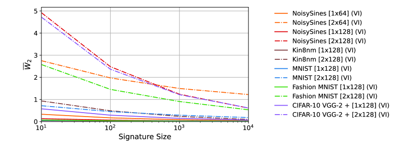
Figure 5: The formal bounds on the relative 2-Wasserstein distance between various SNNs and their Gaussian Mixture approximations obtained via Algorithm 1 for a compression size ($M$) of $3$ and different signature sizes. The plotted lines show the average of 100 random test points.

Uniform Convergence

We continue our analysis with Figure 5, where we conduct an extensive analysis of how the formal error bound from Theorem 13 changes with increasing the signature size for various SNN architectures trained on both regression and classification datasets. The plot confirms that with increasing signature sizes, the approximation error, measured as $\overline{W}_{2}$, tends to decrease uniformly. In particular, we observe an inverse linear rate of convergence, which is consistent with the theoretical asymptotic results established in Graf and Luschgy (2007) on the convergence rates of the Wasserstein distance from signatures for increasing signature size.

Compression Size:		1	3	No Compression
NoisySines	[2x64] (VI)	1.97279	1.63519	1.08763
	[2x128] (VI)	2.48109	2.48488	2.48398
Kin8nm	[2x128] (VI)	0.48740	0.46303	0.45387
MNIST	[2x128] (VI)	0.45036	0.44873	0.44873
Fashion MNIST	[2x128] (VI)	1.45489	1.45466	1.45466
CIFAR-10	VGG-2 + [2x128] (VI)	2.36616	2.35686	2.35686
Compression Size:		10	100	10000
MNIST	[1x64] (Drop)	0.94371	0.73682	0.3571
	[2x64] (Drop)	1.37594	1.09053	0.89742
CIFAR-10	VGG-2 (Drop) + [1x32] (VI)	179.9631	180.0963	145.2984

Table 3: The formal bounds on the relative 2-Wasserstein distance between various SNNs and their Gaussian Mixture approximates obtained via Algorithm 1 for a signature size of $100$ and different compression sizes (M). The reported values are the average of 100 random test points.

In Table 3, we investigate the other approximation step: the compression operation, which reduces the components of the approximation mixtures (step e in Figure 2). The results show that while the networks trained solely with VI can be well approximated with single Gaussian distributions, the precision of the approximation for the networks employing dropout strongly improves with increasing compression size. This confirms that the distribution of these networks is highly multi-modal and underscores the importance of allowing for multi-modal approximations, such as Gaussian mixtures.

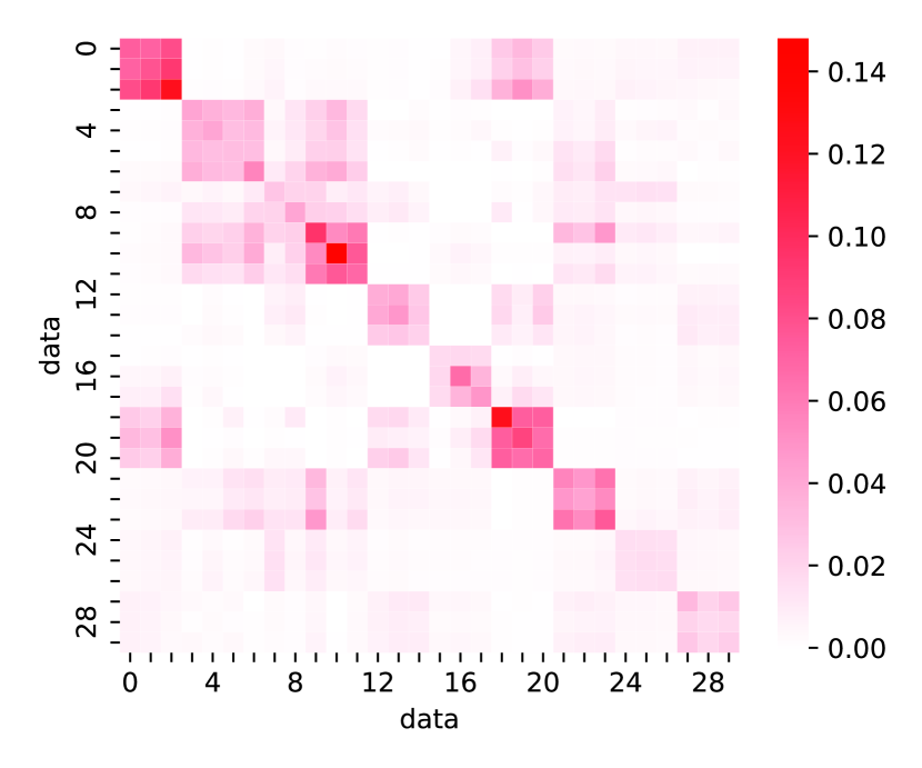
(a) Kernel SNN

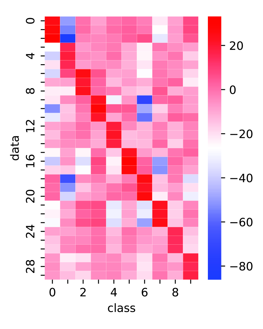
(b) Mean SNN

(c) Kernel GMM

(d) Mean GMM

(I) [2x128] (VI) trained on MNIST

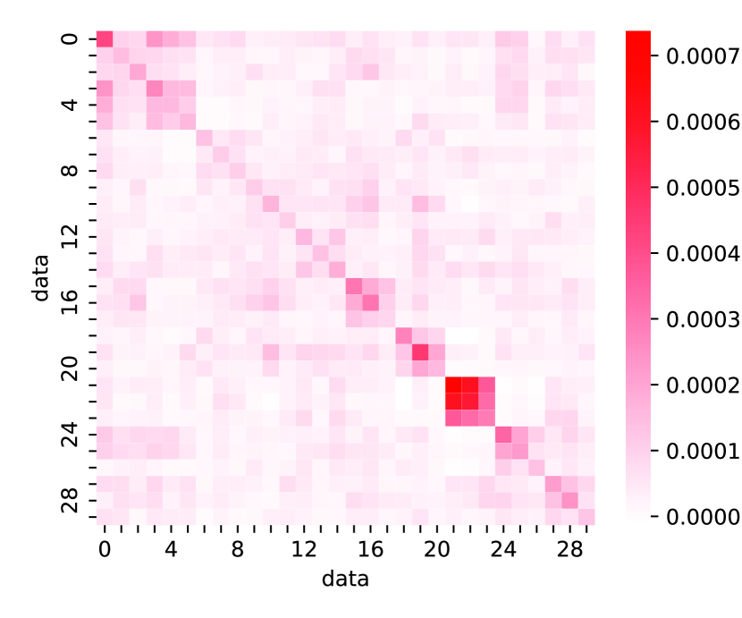
(a) Kernel SNN

(b) Mean SNN

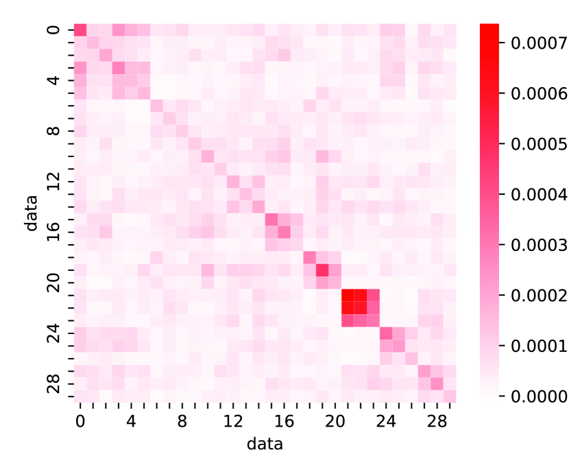
(c) Kernel GMM

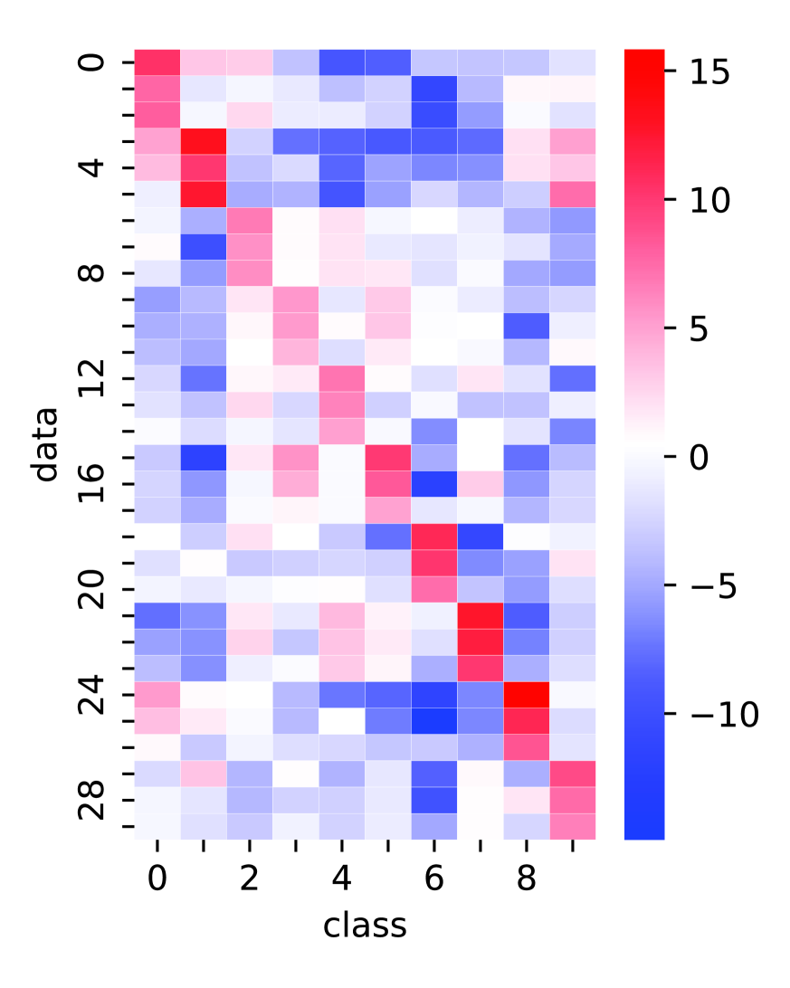
(d) Mean GMM

(II) VGG-2 + [1x128] (VI) trained on CIFAR-10

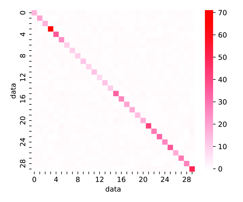
(a) Kernel SNN

(b) Mean SNN

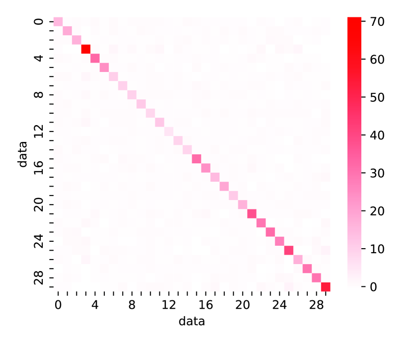
(c) Kernel GMM

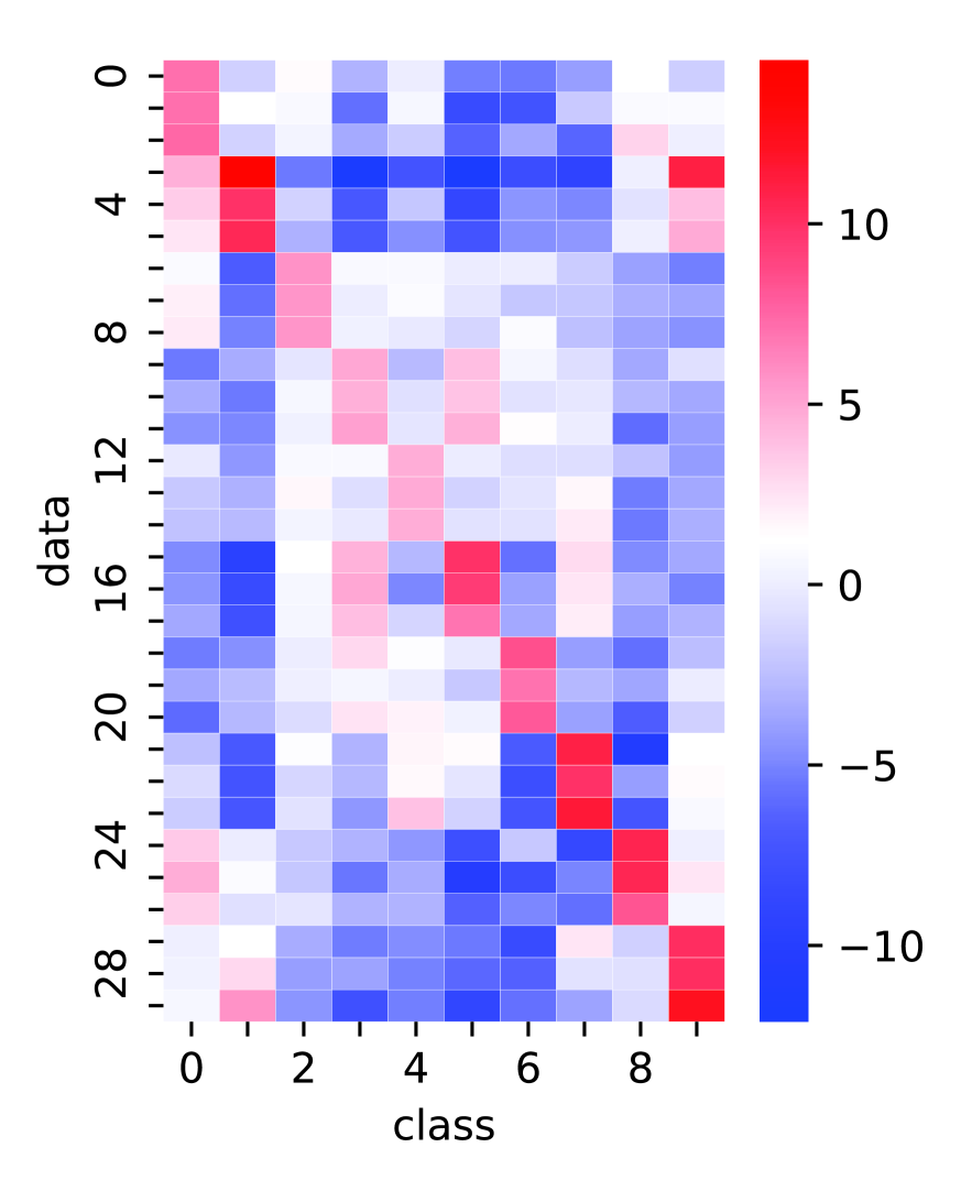
(a) (d) Mean GMM

(III) VGG-2 (Drop) + [1x128] (Drop) trained on CIFAR-10

Figure 6: Kernels and means for various SNNs obtained via Monte Carlo sampling (left two columns) and of our GMM approximation (right two columns) for $30$ input points on MNIST in (I) and CIFAR-10 in (II) and (III). Instead of the full kernel matrices, which have dimensionality $300\times 300$, we store the trace of the sub-blocks in the output dimension, and show the $30\times 30$ matrix that captures the covariance between the input points. The rows and columns are grouped according to the classes, where the colored regions on the y-axis in the mean plots mark the classes. (I) shows the approximate kernels and the predictive means for a fully connected SNN trained via VI, which gives 98% test accuracy. We see in the kernel that examples with the same class labels are correlated. In (II), the VGG network with dropout is combined with a linear stochastic layer on the more complex CIFAR-10 data set, where we obtain 65% accuracy. (III) shows VGG stacked with a linear layer to which we both apply dropout and obtain 64% accuracy on CIFAR-10.

8.2 Posterior Performance Analysis of SNNs

The GMM approximations obtained by Algorithm 1 naturally allow us to visualize the mean and covariance matrix (i.e., kernel) of the predictive distribution at a set of points. The resulting kernel offers the ability to reason about our confidence on the predictions and enhance our understanding of SNN performances (Khan et al., 2019). The state-of-the-art for estimating such a kernel is to rely on Monte Carlo sampling (Van Amersfoort et al., 2020), which, however, is generally time-consuming due to the need to consider a large amount of samples for obtaining accurate estimates.

In Figure 6, we compare the mean and covariance of various SNNs (obtained via Monte Carlo sampling using $1e4$ samples) and the relative GMM approximation on a set of $30$ randomly collected input points for various neural network architectures on the MNIST and CIFAR-10 datasets. We observe that the GMMs match the MC approximation of the true mean and kernel. However, unlike the GMM approximations, the MC approximations lack formal guarantees of correctness, and additionally, computing the MC approximations is generally two orders of magnitudes slower than computing the GMM approximations. By analyzing Figure 6, it is possible to observe that since the architectures allow for the training of highly accurate networks, each row in the posterior mean reflects that the classes are correctly classified. For the networks trained using VI, the kernel matrix clearly shows the correlations trained by the SNN. For the dropout network, the GMM visualizes the limitations of dropout learning in capturing correlation among data points. This finding aligns with the result in Gal and Ghahramani (2016), which shows that Bayesian inference via dropout is equivalent to VI inference with an isotropic Gaussian over the weights per layer.

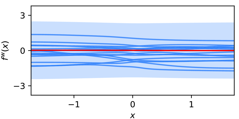
(a) Uninformative SNN Prior

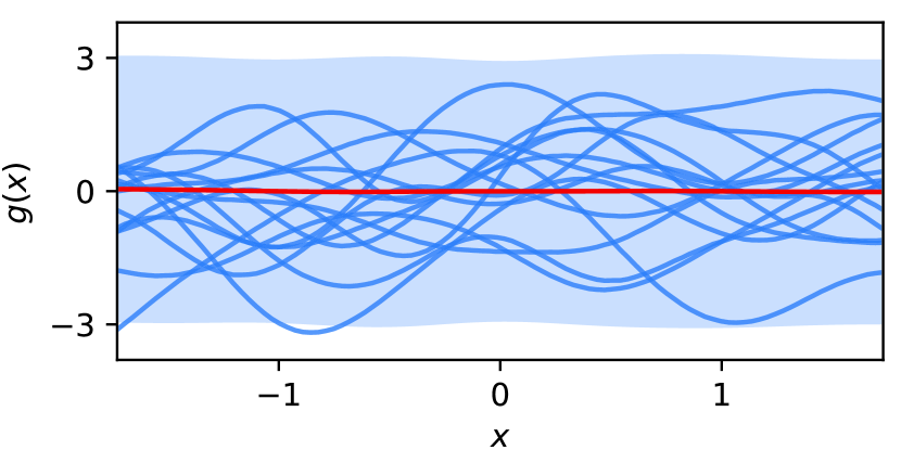
(b) GP Prior

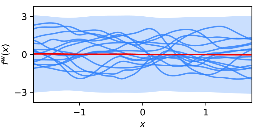
(c) GP Induced SNN Prior (Ours)

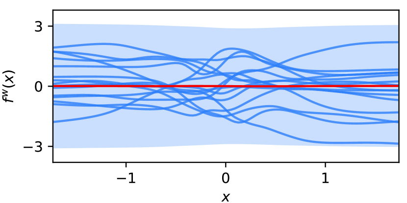
(d) GP Induced SNN Prior (Tran et al., 2022)

Figure 7: Visualization of the prior distribution of (a) a SNN with an isotropic Gaussian distribution over its weights; (b) a zero mean GP with the RBF kernel; (c-d) SNNs with a Gaussian distribution over its weight that is optimized to mimic the GP in (b) via, respectively, our framework and the approach proposed in Tran et al. (2022). The SNN has 2 hidden layers, 128 neurons per layer, and the tanh activation function, while the GP has zero mean and a RBF kernel with length-scale $0.5$ and signal variance $1$. The red lines, blue shaded region, and blue lines respectively indicate the mean, $99.7\%$ credible intervals, and a subset of the MC samples from the output distributions.

8.3 Functional priors for neural networks via GMM approximation

In this section, to highlight another application of our framework, we show how our results can be used to encode functional priors in SNNs. We start from Figure 7(a), where we plot functions sampled from a two hidden layer SNN with an isotropic Gaussian distribution over its weights, which is generally the default choice for priors in Bayesian learning (Fortuin, 2022). As it is possible to observe in the figure, the sampled functions tend to form straight horizontal lines; this is a well-known pathology of neural networks, which becomes more and more exacerbated with deep architectures (Duvenaud et al., 2014), Instead, one may want to consider a prior model that reflects certain characteristics that we expect from the underlying true function, e.g., smoothness or oscillatory behavior. Such characteristics are commonly encoded via a Gaussian process with a given mean and kernel (Tran et al., 2022), as shown for instance in Figure 7(b), where we plot samples from a GP with zero mean and the RBF kernel (MacKay, 1996). We now demonstrate how our framework can be used to encode an informative functional prior, represented as a GP, into a SNN. In particular, in what follows, we assume centered Mean-Field Gaussian priors on the weights, i.e., $p_{{w}}=\mathcal{N}({{\bar{0}}},\mathrm{diag}(\psi))$, where $\psi$ is a vector of possibly different parameters representing the variance of each weight. Our objective is to optimize $\psi$ to minimize the 2-Wasserstein distance between the distributions of the GP and the SNN at a finite set of input points, which we do by following the approach described in Section 7.2. For the low-dimensional 1D regression problem, the input points contain uniform samples in the input domain. For the high-dimensional UCI problems, we use the training sets augmented with noisy samples. We solve the optimization problem as described in Section 7.2, setting $\beta$ to $0.01$, using mini-batch gradient descent with randomly sampled batches.

Length-Scale RBF Kernel	Network Architecture	Uninformative Prior	GP Induced Prior (Tran et al., 2022)	GP Induced Prior (Ours)
1	[2x64]	0.97	0.30	0.25
	[2x128]	0.46	0.30	0.25
0.75	[2x64]	1.09	0.39	0.32
	[2x128]	0.56	0.39	0.31
0.5	[2x64]	1.23	0.53	0.47
	[2x128]	0.69	0.53	0.43

Table 4: The empirical estimates of the relative 2-Wasserstein distance between the prior distributions of zero-mean GPs with the RBF kernel and SNNs with uninformative or GP-induced priors over the weights, at a subset of $20$ points from the test set. The GP-induced prior are either obtained via Algorithm 1 with signatures of size $10$ and compression size (M) of $1$ as described in Section 7.2, or via the method in Tran et al. (2022).

1D Regression Benchmark

We start our analysis with the 1D example in Figure 7, where we compare our framework with the state-of-the-art approach for prior tuning by Tran et al. (2022). Figure 7(c) demonstrates the ability of our approach to encode the oscillating behavior of the GP in the prior distribution of the SNN. In contrast, the SNN prior obtained using the method in Tran et al. (2022) in Figure 7(d) is visually less accurate in capturing the correlation imposed by the RBF kernel of the GP. The performance difference can be explained by the fact that Tran et al. (2022) optimize the 1-Wasserstein distance between the GP and SNN, which relates to the closeness in the first moment (the mean), as they rely on its dual formulation. In contrast, we optimize for the 2-Wasserstein distance, which relates to the closeness in the second moment, including both mean and correlations (see Lemma 2). In Table 4, we investigate the quantitative difference in relative 2-Wasserstein distance between the prior distributions of the GP and SNN in Figure 7, among other network architectures and GP settings. The results show that our method consistently outperforms Tran et al. (2022) on all considered settings.

UCI Regression Benchmark

We continue our analysis on several UCI regression datasets to investigate whether SNNs with an informative prior lead to improved posterior performance compared to uninformative priors. We evaluate the impact of an informative prior on the predictive performance of SNNs using the root-mean-square error (RMSE) and negative log-likelihood (NLL) metrics. The RMSE solely measures the accuracy of the mean predictions, whereas the NLL evaluates whether the predicted distribution matches the actual distribution of the outcomes, taking into account the uncertainty of the predictions. Lower RMSE and NLL values indicate better performance. Figure 8 shows that for all datasets, the GP outperforms the SNN with an uninformative prior both in terms of mean and uncertainty accuracy. By encoding the GP prior in the SNN, we can greatly improve the predictive performance of the SNN, bringing it closer to the performance of the GP. The remaining performance gap to the GP can be explained by the VI error in approximating the posterior distribution.

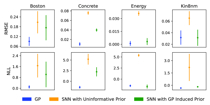
Figure 8: Report of the predictive performance of a GP with zero-mean and RBF kernel, and a $[2\times 128]$ SNN with tanh activation function on several UCI regression datasets in terms of the root-mean-squared error (RMSE) and negative log-likelihood (NLL). The dots and bars represent the means and standard deviations over the 10 random test splits of the datasets, respectively. The results for the GP are shown in blue, the results for the SNN with an uninformative isotropic Gaussian prior on the weights are in yellow, and the results for the SNN with the GP-induced informative priors obtained via our approach are in green.

9 Conclusion

We introduced a novel algorithmic framework to approximate the input-output distribution of a SNN with a GMM, providing bounds on the approximation error in terms of the Wasserstein distance. Our framework relies on techniques from quantization theory and optimal transport, and is based on a novel approximation scheme for GMMs using signature approximations. We performed a detailed theoretical analysis of the error introduced by our GMM approximations and complemented the theoretical analysis with extensive empirical validation, showing the efficacy of our methods in both regression and classification tasks, and for various applications, including prior selection and uncertainty quantification. We should stress that in this paper we focused on finding GMM approximations of neural networks at a finite set of input points, thus also accounting for the correlations among these points. While reasoning for a finite set of input points is standard in stochastic approximations (Yaida, 2020; Basteri and Trevisan, 2024) and has many applications, as also highlighted in the paper, for some other applications, such as adversarial robustness of Bayesian neural networks (Wicker et al., 2020), one may require approximations that are valid for compact sets of input points. We believe this is an interesting future research question.

Appendix A Proofs

We present the proofs for all results discussed in the main text of this work. These proofs rely on several less commonly reported properties of the Wasserstein distance, which we will first discuss in Section A.1. After this, we present the proofs ordered per section.

A.1 Properties of the Wasserstein Distance

Lemma 23 (2-Wasserstein Distance for Independent Joint Distributions)

Let $p,q\in{\mathcal{P}}({\mathbb{R}}^{n})$ be joint distributions that are independent over each dimension, i.e., $p=\prod_{i=1}^{n}{p^{{(i)}}}$ and $q=\prod_{i=1}^{n}{q^{{(i)}}}$, where ${p^{{(i)}}}$ and ${q^{{(i)}}}$ are the marginal distributions of $p$ and $q$ for the $i$-th dimension, respectively. Then, we have that:

$${\mathbb{W}}_{2}^{2}(p,q)=\sum_{i=1}^{n}{\mathbb{W}}_{2}^{2}({p^{{(i)}}},{q^{{(i)}}}).$$

Proof  Due to $p$ and $q$ being independent over each dimension, we have:

$${\mathbb{W}}_{2}^{2}(p,q) =\inf_{\gamma\in\Gamma(p,q)}{\mathbb{E}}_{({{x}},{{y}})\sim\gamma}[\|{{x}}-{{y}}\|^{2}]$$

$$=\inf_{\gamma\in\Gamma(p,q)}\sum_{i=1}^{n}{\mathbb{E}}_{({{x}},{{y}})\sim\gamma}[({{{x}}^{(i)}}-{{{y}}^{(i)}})^{2}]$$

$$=\inf_{\gamma\in\Gamma(p,q)}\sum_{i=1}^{n}{\mathbb{E}}_{({{{x}}^{(i)}},{{{y}}^{(i)}})\sim{\gamma^{{(i)}}}}[({{{x}}^{(i)}}-{{{y}}^{(i)}})^{2}],$$

where the set of couplings can be rewritten as

$$\Gamma(p,q)=\Gamma\left(\prod_{i=1}^{n}{p^{{(i)}}},\prod_{i=1}^{n}{q^{{(i)}}}\right)=\prod_{i=1}^{n}\Gamma({p^{{(i)}}},{q^{{(i)}}}),$$

such that

$$\inf_{\gamma\in\Gamma(p,q)}\sum_{i=1}^{n}{\mathbb{E}}_{({{{x}}^{(i)}},{{{y}}^{(i)}})\sim{\gamma^{{(i)}}}}[({{{x}}^{(i)}}-{{{y}}^{(i)}})^{2}] =\sum_{i=1}^{n}\inf_{{\gamma^{{(i)}}}\in\Gamma({p^{{(i)}}},{q^{{(i)}}})}{\mathbb{E}}_{({{{x}}^{(i)}},{{{y}}^{(i)}})\sim{\gamma^{{(i)}}}}[({{{x}}^{(i)}}-{{{y}}^{(i)}})^{2}]$$

$$=\sum_{i=1}^{n}{\mathbb{W}}_{2}^{2}({p^{{(i)}}},{q^{{(i)}}})$$

 

Proposition 24

(Upper Bound on the Wasserstein Distance between Mixtures Distributions, a Generalization of Proposition 4 in Delon and Desolneux (2020)) Let $\sum_{i=1}^{M}{{{\pi}}_{p}^{{(i)}}}p_{i}\in{\mathcal{P}}_{2}({\mathbb{R}}^{d})$ and $\sum_{j=1}^{N}{{{\pi}}_{q}^{{(j)}}}q_{j}\in{\mathcal{P}}_{2}({\mathbb{R}}^{d})$ be two mixture distributions, and let $\Gamma({{\pi}}_{p},{{\pi}}_{q})$ be the subset of simplex $\Pi_{M\times N}$ with marginals ${{\pi}}_{p}$ and ${{\pi}}_{q}$. Then for any $\bar{{{\pi}}}\in\Gamma({{\pi}}_{p},{{\pi}}_{q})$, it holds that:

$${\mathbb{W}}_{2}^{2}\left(\sum_{i=1}^{M}{{{\pi}}_{p}^{{(i)}}}p_{i},\sum_{j=1}^{N}{{{\pi}}_{q}^{{(j)}}}q_{j}\right)\leq\sum_{i=1}^{M}\sum_{j=1}^{N}{\bar{{{\pi}}}^{{(i,j)}}}{\mathbb{W}}_{2}^{2}(p_{i},q_{j}).$$

Proof  Recall that according to the definition of the 2-Wasserstein distance:

$${\mathbb{W}}_{2}^{2}\left(\sum_{i=1}^{M}{{{\pi}}_{p}^{{(i)}}}p_{i},\sum_{j=1}^{N}{{{\pi}}_{q}^{{(j)}}}q_{j}\right)=\inf_{\gamma\in\Gamma\left(\sum_{i=1}^{M}{{{\pi}}_{p}^{{(i)}}}p_{i},\sum_{j=1}^{N}{{{\pi}}_{q}^{{(j)}}}q_{j}\right)}{\mathbb{E}}_{({{z}},\tilde{{{z}}})\sim\gamma}[\|{{z}}-\tilde{{{z}}}\|^{2}],$$

where $\Gamma\left(\sum_{i=1}^{M}{{{\pi}}_{p}^{{(i)}}}p_{i},\sum_{j=1}^{N}{{{\pi}}_{q}^{{(j)}}}q_{j}\right)$ represents the set of all joint probability distributions with marginal distributions $\sum_{i=1}^{M}{{{\pi}}_{p}^{{(i)}}}p_{i}$ and $\sum_{j=1}^{N}{{{\pi}}_{q}^{{(j)}}}q_{j}$. Consider the following subset of joint distributions

$$\bar{\Gamma}\coloneqq\bigg{\{}\sum_{i=1}^{M}\sum_{j=1}^{N}{\bar{{{\pi}}}^{{(i,j)}}}\gamma\mid\bar{{{\pi}}}\in\Gamma({{\pi}}_{p},{{\pi}}_{q}),\gamma\in\Gamma(p_{i},q_{j})\bigg{\}}\subset\Gamma\left(\sum_{i=1}^{M}{{{\pi}}_{p}^{{(i)}}}p_{i},\sum_{j=1}^{N}{{{\pi}}_{q}^{{(j)}}}q_{j}\right).$$

It follows that:

$$\inf_{\gamma\in\Gamma\left(\sum_{i=1}^{M}{{{\pi}}_{p}^{{(i)}}}p_{i},\sum_{j=1}^{N}{{{\pi}}_{q}^{{(j)}}}q_{j}\right)}{\mathbb{E}}_{({{z}},\tilde{{{z}}})\sim\gamma}[\|{{z}}-\tilde{{{z}}}\|^{2}] \leq\inf_{\gamma\in\bar{\Gamma}}{\mathbb{E}}_{({{z}},\tilde{{{z}}})\sim\gamma}[\|{{z}}-\tilde{{{z}}}\|^{2}]$$

$$=\sum_{i=1}^{M}\sum_{j=1}^{N}{\bar{{{\pi}}}^{{(i,j)}}}\inf_{\gamma\in\Gamma(p_{i},q_{j})}{\mathbb{E}}_{({{z}},\tilde{{{z}}})\sim\gamma}[\|{{z}}-\tilde{{{z}}}\|^{2}]$$

$$=\sum_{i=1}^{M}\sum_{j=1}^{N}{\bar{{{\pi}}}^{{(i,j)}}}{\mathbb{W}}_{2}^{2}(p_{i},q_{j}),$$

which completes the proof.  

A.2 Proofs Section 5

Proposition 8: Optimal Transport Plan for Wasserstein Distance Between Distributions and Their Signatures

Proof  The proof follows directly from Theorem 1 in (Ambrogioni et al., 2018). According to this theorem, for any $\rho\in\mathbb{N}$, we have that

$${\mathbb{W}}_{\rho}^{\rho}(p,{\Delta}_{\mathcal{C}}\#p)=\sum_{i=1}^{N}{{{\pi}}^{(i)}}{\mathbb{E}}_{{{z}}\sim p}[\|{{z}}-{{c}}_{i}\|^{\rho}\mid{{z}}\in{\mathcal{R}}_{i}].$$

 

Proposition 9: Wasserstein Distance from Signatures of Univariate Gaussians

Proof  From Proposition 8, we have that

$${\mathbb{W}}_{2}^{2}({\Delta}_{{\mathcal{C}}}\#\mathcal{N}(0,1),\mathcal{N}(0,1)) =\sum_{i=1}^{N}\Phi_{i}{\mathbb{E}}_{z\sim\mathcal{N}(0,1)}[({{z}}-c_{i})^{2}\mid z\in[l_{i},u_{i}]].$$

where $\Phi_{i}=\mathbb{P}_{z\sim\mathcal{N}(0,1)}[z\in[l_{i},u_{i}]]$. Using the probability density function (pdf) of the Gaussian distribution and a simple change of variables, we can write conditional expectation terms as:

$${\mathbb{E}}_{z\sim\mathcal{N}(0,1)}[({{z}}-c_{i})^{2}\mid z\in[l_{i},u_{i}]] =\frac{1}{\Phi_{i}}\int(z-c_{i})^{2}{\mathbf{1}}_{[l_{i},u_{i}]}(z)\mathcal{N}(z\mid 0,1)dz,$$

$$=\frac{1}{\Phi_{i}}\int z^{2}{\mathbf{1}}_{[l_{i}-c_{i},u_{i}-c_{i}]}(z)\mathcal{N}(z\mid-c_{i},1)dz$$

where $\mathcal{N}(z\mid-c_{i},1)$ denotes the pdf of a Gaussian distribution with mean $-c_{i}$ and variance $1$, and ${\mathbf{1}}_{[l,u]}(z)$ is the indicator function which equals $1$ if $z\in[l,u]$ and $0$ otherwise. Note that, $\frac{1}{\Phi_{i}}{\mathbf{1}}_{[l_{i}-c_{i},u_{i}-c_{i}]}(z)\mathcal{N}(z\mid-c_{i},1)$ is in fact the pdf of a random variable with a Gaussian distribution $\mathcal{N}(-c_{i},1)$ conditioned on $[l_{i}-c_{i},u_{i}-c_{i}]$. Hence, the above conditional expectation is equivalent to the second moment of a truncated Gaussian random variable on $[l_{i}-c_{i},u_{i}-c_{i}]$, for which closed-form expressions exist (Wilhelm et al., 2012). Following Section 3 of Wilhelm et al. (2012) we can write:

$$\frac{1}{\Phi_{i}}\int z^{2}{\mathbf{1}}_{[l_{i}-c_{i},u_{i}-c_{i}]}(z)\mathcal{N}(z\mid-c_{i},1)dz =\frac{\nu_{i}+(\mu_{i}-c_{i})^{2}}{\Phi_{i}}.$$

Thus, we finally obtain:

$$\sum_{i=1}^{N}\Phi_{i}{\mathbb{E}}_{{{z}}\sim\mathcal{N}(0,1)}[\|{{z}}-c_{i}\|^{2}\mid{{z}}\in[l_{i},u_{i}]]=\sum_{i=1}^{N}\nu_{i}+(\mu_{i}-c_{i})^{2}.$$

 

Corollary 10 of Proposition 9: Wasserstein Distance from Signatures of Multivariate Gaussians

Proof  According to Proposition 8, we have:

$${\mathbb{W}}_{2}^{2}({\Delta}_{\mathcal{C}}\#\mathcal{N}({{\bar{0}}},\Sigma),\mathcal{N}({{\bar{0}}},\Sigma)) =\sum_{i=1}^{N}\mathbb{P}_{{{z}}\sim\mathcal{N}({{\bar{0}}},\Sigma)}[{{z}}\in{\mathcal{R}}_{i}]{\mathbb{E}}_{{{z}}\sim\mathcal{N}({{\bar{0}}},\Sigma)}[\|{{z}}-{{c}}_{i}\|^{2}\mid{{z}}\in{\mathcal{R}}_{i}].$$

For all $i\in\{1,\ldots,N\}$, we can write

$$\mathbb{P}_{{{z}}\sim\mathcal{N}({{\bar{0}}},\Sigma)}[{{z}}\in{\mathcal{R}}_{i}]{\mathbb{E}}_{{{z}}\sim\mathcal{N}({{\bar{0}}},\Sigma)}[\|{{z}}-{{c}}_{i}\|^{2}\mid{{z}}\in{\mathcal{R}}_{i}]$$

$$\qquad\qquad=\mathbb{P}_{{{z}}\sim\mathcal{N}({{\bar{0}}},\Sigma)}[{{z}}\in{\mathcal{R}}_{i}]\int\|\tilde{{{z}}}-{{c}}_{i}\|^{2}\frac{{\mathbf{1}}_{{\mathcal{R}}_{i}}(\tilde{{{z}}})\mathcal{N}(\tilde{{{z}}}\mid{{\bar{0}}},\Sigma)}{\mathbb{P}_{{{z}}\sim\mathcal{N}({{\bar{0}}},\Sigma)}[{{z}}\in{\mathcal{R}}_{i}]}d\tilde{{{z}}}$$

$$\qquad\qquad=\int_{{\mathcal{R}}_{i}}\|{{z}}-{{c}}_{i}\|^{2}\mathcal{N}({{z}}\mid{{\bar{0}}},\Sigma)d{{z}}.$$

By applying substitution ${{q}}={{T}}{{z}}$ to the integral terms, we obtain:

$$\int_{{\mathcal{R}}_{i}}\|{{z}}-{{c}}_{i}\|^{2}\mathcal{N}({{z}}\mid{{\bar{0}}},\Sigma)d{{z}} =\int_{\{{{T}}{{z}}\mid{{z}}\in{\mathcal{R}}_{i}\}}\|{{S}}({{q}}-{{T}}{{c}}_{i})\|^{2}\mathcal{N}({{q}}\mid{{\bar{0}}},{{I}})d{{q}}.$$

Here, since ${\mathcal{C}}$ is a grid in the transformed space induced by ${{T}}$, $\{{{T}}{{z}}\mid{{z}}\in{\mathcal{R}}_{i}\}$ is an axis-aligned hyper-rectangle that can be defined by vectors ${{l}}_{i},{{u}}_{i}\in{\mathbb{R}}^{n}$, i.e., $\{{{T}}{{z}}\mid{{z}}\in{\mathcal{R}}_{i}\}=[{{l}}_{i},{{u}}_{i}]$. Furthermore, because matrix ${{V}}$ is orthogonal, we have:

$$\|{{S}}{{q}}\|^{2}={{q}}^{T}(\mathrm{diag}({{\lambda}})^{-\frac{1}{2}}{{V}}^{T}{{V}}\mathrm{diag}({{\lambda}})^{-\frac{1}{2}})^{-1}{{q}}={{q}}^{T}\mathrm{diag}({{\lambda}}){{q}}=\sum_{l=1}^{n}{{{\lambda}}^{(l)}}{{{q}}^{(l)}}^{2}.$$

Hence, we can write

$$\int_{[{{l}}_{i},{{u}}_{i}]}\|{{S}}({{q}}-{{T}}{{c}}_{i})\|^{2}\mathcal{N}({{q}}\mid{{\bar{0}}},{{I}})d{{q}} =\sum_{l=1}^{n}{{{\lambda}}^{(l)}}\int_{[{{l}}_{i},{{u}}_{i}]}({{{q}}^{(l)}}-{\bar{{{c}}}_{i}^{{(l)}}})^{2}\mathcal{N}({{q}}\mid{{\bar{0}}},{{I}})d{{q}},$$

where $\bar{{{c}}}_{i}={{T}}{{c}}_{i}$. Using that $\mathcal{N}({{q}}\mid{{\bar{0}}},{{I}})=\prod_{l=1}^{n}\mathcal{N}({{{q}}^{(l)}}\mid 0,1)$, we can further simplify the above expression as follows

$$\sum_{l=1}^{n}{{{\lambda}}^{(l)}}\int_{[{{l}}_{i},{{u}}_{i}]}({{{q}}^{(l)}}-{\bar{{{c}}}_{i}^{{(l)}}})^{2}\mathcal{N}({{q}}\mid{{\bar{0}}},{{I}})d{{q}}$$

$$\qquad=\sum_{l=1}^{n}{{{\lambda}}^{(l)}}\Big{(}\prod_{\begin{subarray}{c}j=1\\ j\neq l\end{subarray}}^{n}\int_{{{{l}}_{i}^{{(j)}}}}^{{{{u}}_{i}^{{(j)}}}}1d{{{q}}^{(j)}}\Big{)}\int_{[{{{l}}_{i}^{{(l)}}},{{{u}}_{i}^{{(l)}}}]}({{{q}}^{(l)}}-{{{c}}_{i}^{{(l)}}})^{2}\mathcal{N}({{{q}}^{(l)}}\mid 0,1)d{{{q}}^{(l)}}$$

$$\qquad=\sum_{l=1}^{n}{{{\lambda}}^{(l)}}\Big{(}\prod_{\begin{subarray}{c}j=1\\ j\neq l\end{subarray}}^{n}\mathbb{P}_{{{{q}}^{(j)}}\sim\mathcal{N}(0,1)}[{{{q}}^{(j)}}\in[{{{l}}_{i}^{{(j)}}},{{{u}}_{i}^{{(j)}}}]]\Big{)}\int_{[{{{l}}_{i}^{{(l)}}},{{{u}}_{i}^{{(l)}}}]}({{{q}}^{(l)}}-{{{c}}_{i}^{{(l)}}})^{2}\mathcal{N}({{{q}}^{(l)}}\mid 0,1)d{{{q}}^{(l)}}$$

$$\qquad=\sum_{l=1}^{n}{{{\lambda}}^{(l)}}\Big{(}\prod_{\begin{subarray}{c}j=1\end{subarray}}^{n}\mathbb{P}_{{{{q}}^{(j)}}\sim\mathcal{N}(0,1)}[{{{q}}^{(j)}}\in[{{{l}}_{i}^{{(j)}}},{{{u}}_{i}^{{(j)}}}]]\Big{)}{\mathbb{E}}_{{{{q}}^{(l)}}\sim\mathcal{N}(0,1)}[({{{q}}^{(l)}}-{{{c}}_{i}^{{(l)}}})^{2}\mid{{{q}}^{(l)}}\in[{{{l}}_{i}^{{(l)}}},{{{u}}_{i}^{{(l)}}}]]$$

$$\qquad=\Big{(}\prod_{\begin{subarray}{c}j=1\end{subarray}}^{n}\underbrace{\mathbb{P}_{{{{q}}^{(j)}}\sim\mathcal{N}(0,1)}[{{{q}}^{(j)}}\in[{{{l}}_{i}^{{(j)}}},{{{u}}_{i}^{{(j)}}}]]}_{\eqqcolon{\mathbb{P}_{i}^{{(j)}}}}\Big{)}\sum_{l=1}^{n}{{{\lambda}}^{(l)}}\underbrace{{\mathbb{E}}_{{{{q}}^{(l)}}\sim\mathcal{N}(0,1)}[({{{q}}^{(l)}}-{{{c}}_{i}^{{(l)}}})^{2}\mid{{{q}}^{(l)}}\in[{{{l}}_{i}^{{(l)}}},{{{u}}_{i}^{{(l)}}}]]}_{\eqqcolon{{\mathbb{E}}_{i}^{{(j)}}}}$$

Because of Eqn. (10), without loss of generality, we can set the indexing of the signature locations, and hence the related regions, such that for all $i\in N$:

$$\bar{{{c}}}_{i}=\bar{{{c}}}_{i_{1}\cdot i_{2}\cdot\ldots\cdot i_{n}}=({\bar{{{c}}}_{i_{1}}^{{(1)}}},{\bar{{{c}}}_{i_{2}}^{{(2)}}},\ldots,{\bar{{{c}}}_{i_{n}}^{{(n)}}})^{T},$$

where $i_{l}\in\{1,\ldots,|{\mathcal{C}}^{l}|\}$, and ${\bar{{{c}}}_{i_{l}}^{{(l)}}}\in{\mathcal{C}}^{l}$, $\forall l\in\{1,\ldots,n\}$. Using straightforward algebra, we can now write

$$\sum_{i=1}^{N}\Big{(}\prod_{j=1}^{n}{\mathbb{P}_{i}^{{(j)}}}\Big{)}\Big{(}\sum_{l=1}^{n}{{\mathbb{E}}_{i}^{{(l)}}}\Big{)} =\sum_{i_{1}=1}^{|{\mathcal{C}}^{1}|}\sum_{i_{2}=1}^{|{\mathcal{C}}^{2}|}\ldots\sum_{i_{n}=1}^{|{\mathcal{C}}^{n}|}\Big{(}\prod_{j=1}^{n}{\mathbb{P}_{i_{1}\cdot i_{2}\ldots\cdot i_{n}}^{{(j)}}}\Big{)}\Big{(}\sum_{l=1}^{n}{{\mathbb{E}}_{i_{1}\cdot i_{2}\ldots\cdot i_{n}}^{{(l)}}}\Big{)}$$

$$=\sum_{i_{1}=1}^{|{\mathcal{C}}^{1}|}{\mathbb{P}_{i_{1}\cdot i_{2}\ldots\cdot i_{n}}^{{(1)}}}\sum_{i_{2}=1}^{|{\mathcal{C}}^{2}|}{\mathbb{P}_{i_{1}\cdot i_{2}\ldots\cdot i_{n}}^{{(2)}}}\ldots\sum_{i_{n}=1}^{|{\mathcal{C}}^{n}|}{\mathbb{P}_{i_{1}\cdot i_{2}\ldots\cdot i_{n}}^{{(n)}}}\sum_{l=1}^{n}{{\mathbb{E}}_{i_{1}\cdot i_{2}\ldots\cdot i_{n}}^{{(l)}}}$$

$$=\sum_{l=1}^{n}\Big{(}\prod_{\begin{subarray}{c}k=1\\ k\neq l\end{subarray}}^{n}\sum_{i_{k}=1}^{|{\mathcal{C}}^{k}|}{\mathbb{P}_{i_{1}\cdot i_{2}\ldots\cdot i_{n}}^{{(k)}}}\Big{)}\Big{(}\sum_{i_{l}=1}^{|{\mathcal{C}}^{l}|}{\mathbb{P}_{i_{1}\cdot i_{2}\ldots\cdot i_{n}}^{{(l)}}}{{\mathbb{E}}_{i_{1}\cdot i_{2}\ldots\cdot i_{n}}^{{(l)}}}\Big{)}$$

Note that, as a consequence of our indexing, $\cup_{i_{k}=1}^{|{\mathcal{C}}^{k}|}[{{{l}}_{\ldots\cdot i_{k}\cdot\ldots}^{{(k)}}},{{{u}}_{\ldots\cdot i_{k}\cdot\ldots}^{{(k)}}}]={\mathbb{R}}$, and hence

$$\sum_{i_{k}=1}^{|{\mathcal{C}}^{k}|}{\mathbb{P}_{\ldots\cdot i_{k}\cdot\ldots}^{{(k)}}}=\sum_{i_{k}=1}^{|{\mathcal{C}}^{k}|}\mathbb{P}_{{{{q}}^{(k)}}\sim\mathcal{N}(0,1)}[{{{q}}^{(k)}}\in[{{{l}}_{\ldots\cdot i_{k}\cdot\ldots}^{{(k)}}},{{{u}}_{\ldots\cdot i_{k}\cdot\ldots}^{{(k)}}}]]=1.$$

Furthermore for $l\in\{1,\ldots,n\}$,

$$\sum_{i_{l}=1}^{|{\mathcal{C}}^{l}|}{\mathbb{P}_{\ldots\cdot i_{l}\cdot\ldots}^{{(l)}}}{{\mathbb{E}}_{\ldots\cdot i_{k}\cdot\ldots}^{{(l)}}}$$

$$\qquad={{{\lambda}}^{(l)}}\sum_{i_{l}=1}^{|{\mathcal{C}}^{k}|}\mathbb{P}_{{{{q}}^{(l)}}\sim\mathcal{N}(0,1)}[{{{q}}^{(l)}}\in[{{{l}}_{\ldots\cdot i_{l}\cdot\ldots}^{{(l)}}},{{{u}}_{\ldots\cdot i_{l}\cdot\ldots}^{{(l)}}}]]{\mathbb{E}}_{{{{q}}^{(l)}}\sim\mathcal{N}(0,1)}[({{{q}}^{(l)}}-{\bar{{{c}}}_{\ldots\cdot i_{l}\cdot\ldots}^{{(l)}}})^{2}\mid{{{q}}^{(l)}}\in[{{{l}}_{\ldots\cdot i_{l}\cdot\ldots}^{{(l)}}},{{{u}}_{\ldots\cdot i_{l}\cdot\ldots}^{{(l)}}}]]$$

$$\qquad={{{\lambda}}^{(l)}}{\mathbb{W}}_{2}^{2}({\Delta}_{{\bar{{\mathcal{C}}}^{{(l)}}}}\#\mathcal{N}(0,1),\mathcal{N}(0,1)).$$

Combining the above results, we obtain:

$${\mathbb{W}}_{2}^{2}({\Delta}_{\mathcal{C}}\#\mathcal{N}({{\bar{0}}},\Sigma),\mathcal{N}({{\bar{0}}},\Sigma)) =\sum_{l=1}^{n}\Big{(}\prod_{\begin{subarray}{c}k=1\\ k\neq l\end{subarray}}^{n}\sum_{i_{k}=1}^{|{\mathcal{C}}^{k}|}{\mathbb{P}_{i_{1}\cdot i_{2}\ldots\cdot i_{n}}^{{(k)}}}\Big{)}\Big{(}\sum_{i_{l}=1}^{|{\mathcal{C}}^{l}|}{\mathbb{P}_{i_{1}\cdot i_{2}\ldots\cdot i_{n}}^{{(l)}}}{{\mathbb{E}}_{i_{1}\cdot i_{2}\ldots\cdot i_{n}}^{{(l)}}}\Big{)}$$

$$=\sum_{l=1}^{n}\Big{(}\prod_{\begin{subarray}{c}k=1\\ k\neq l\end{subarray}}^{n}1)\Big{(}{{{\lambda}}^{(l)}}{\mathbb{W}}_{2}^{2}({\Delta}_{{\bar{{\mathcal{C}}}^{{(l)}}}}\#\mathcal{N}(0,1),\mathcal{N}(0,1))\Big{)}$$

$$=\sum_{l=1}^{n}{{{\lambda}}^{(l)}}{\mathbb{W}}_{2}^{2}({\Delta}_{{\bar{{\mathcal{C}}}^{{(l)}}}}\#\mathcal{N}(0,1),\mathcal{N}(0,1)).$$

To conclude the proof, note that for non-zero mean, we can follow the same procedure but apply substitution $q={{T}}({{x}}-{m})$ and define $\bar{{{c}}}={{T}}({{c}}-{m})$.  

A.3 Proofs Section 6

Lemma 14: Bounds on the Spectral Norm of Random Matrices with Correlated Elements

Proof  We here generalize the result presented in the main text, and prove that for both $\rho=2$ and $\rho=1$:

$${\mathbb{E}}_{{{W}}\sim p_{{W}}}[\|{{W}}\|^{\rho}]^{\frac{1}{\rho}} \leq\Big{(}\sum_{i,j}{\mathbb{E}}_{\bar{{{W}}}\sim\bar{p}_{{W}}}[({\bar{{{W}}}^{{(i,j)}}})^{2}]\Big{)}^{\frac{1}{2}}+\|{{M}}\|.$$ (30)

Using the triangle inequality for the spectral norm, we have

$${\mathbb{E}}_{{{W}}\sim p_{{W}}}[\|{{W}}\|]={\mathbb{E}}_{\bar{{{W}}}\sim\bar{p}_{{W}}}[\|\bar{{{W}}}+{{M}}\|]\leq{\mathbb{E}}_{\bar{{{W}}}\sim\bar{p}_{{W}}}[\|\bar{{{W}}}\|]+\|{{M}}\|$$

Using Minkowski’s inequality for the spectral norm, we get

$${\mathbb{E}}_{{{W}}\sim p_{{W}}}[\|{{W}}\|^{2}]^{\frac{1}{2}} ={\mathbb{E}}_{\bar{{{W}}}\sim\bar{p}_{{W}}}[\|\bar{{{W}}}+{{M}}\|^{2}]^{\frac{1}{2}}$$

$$\leq{\mathbb{E}}_{\bar{{{W}}}\sim\bar{p}_{{W}}}[\|\bar{{{W}}}\|^{2}]^{\frac{1}{2}}+\|{{M}}\|$$

For any matrix $\bar{{{W}}}\in{\mathbb{R}}^{n\times m}$, we have $\|\bar{{{W}}}\|\leq\|\bar{{{W}}}\|_{\mathcal{F}}$, where $\|\cdot\|_{\mathcal{F}}$ denotes the Frobenius defined by $\|\bar{{{W}}}\|_{\mathcal{F}}^{2}=\sum_{i,j}({\bar{{{W}}}^{{(i,j)}}})^{2}$. Therefore,

$${\mathbb{E}}_{\bar{{{W}}}\sim\bar{p}_{{W}}}[\|\bar{{{W}}}\|^{2}]^{\frac{1}{2}}\leq{\mathbb{E}}_{\bar{{{W}}}\sim\bar{p}_{{W}}}[\|\bar{{{W}}}\|_{\mathcal{F}}^{2}]^{\frac{1}{2}}\leq\Big{(}\sum_{i,j}{\mathbb{E}}_{\bar{{{W}}}\sim\bar{p}_{{W}}}[({\bar{{{W}}}^{{(i,j)}}})^{2}]\Big{)}^{\frac{1}{2}}.$$

This concludes the proof for $\rho=2$. For $\rho=1$, we additionally apply Jensen’s inequality:

$${\mathbb{E}}_{\bar{{{W}}}\sim\bar{p}_{{{W}}}}[\|{{W}}\|]\leq{\mathbb{E}}_{\bar{{{W}}}\sim\bar{p}_{{{W}}}}[\|{{W}}\|_{\mathcal{F}}]\leq{\mathbb{E}}_{\bar{{{W}}}\sim\bar{p}_{{W}}}\Big{[}\Big{(}\sum_{i,j}({\bar{{{W}}}^{{(i,j)}}})^{2}\Big{)}^{\frac{1}{2}}\Big{]}\leq\Big{(}\sum_{i,j}{\mathbb{E}}_{\bar{{{W}}}\sim\bar{p}_{{W}}}[({\bar{{{W}}}^{{(i,j)}}})^{2}]\Big{)}^{\frac{1}{2}}.$$

 

Results in Table 11: Wasserstein Distance under Push-Forward Operations in SNNs

Proposition 25 (Wasserstein Distance under Stochastic Linear Operations)

Let
$L_{{{w}}}:{\mathbb{R}}^{n}\rightarrow{\mathbb{R}}^{m}$ be the affine operation $L_{{w}}({{z}})={{W}}{{z}}+{{b}}$ with parameters ${{W}}\in{\mathbb{R}}^{n\times m}$ and ${{b}}\in{\mathbb{R}}^{m}$. Further, assume a distribution $p_{{w}}\in{\mathcal{P}}({\mathbb{R}}^{(n+1)\times m})$ over ${{w}}=({{W}},{{b}})$ such that for any ${{z}}\in{\mathbb{R}}^{n}$, the random variable $L_{{w}}({{z}})$ follows the probability distribution $p_{L_{{w}}({{z}})}=L_{{{w}}}({{z}})\#p_{{w}}$. Then, for $\rho\in\{1,2\}$ and probability distributions $p,q\in{\mathcal{P}}_{\rho}({\mathbb{R}}^{n})$ it holds that

$${\mathbb{W}}_{\rho}({\mathbb{E}}_{{{z}}\sim p}[p_{L_{{w}}({{z}})}],{\mathbb{E}}_{\tilde{{{z}}}\sim q}[p_{L_{{w}}(\tilde{{{z}}})}])\leq{\mathbb{E}}_{({{W}},{{b}})\sim p_{w}}[\|{{W}}\|^{\rho}]^{\frac{1}{\rho}}{\mathbb{W}}_{\rho}(p,q).$$ (31)

Proof  Since the spectral (matrix) norm, denoted as $\|\cdot\|$, is consistent with the Euclidean vector-norm, we have that $\|{{W}}{{z}}-{{W}}\tilde{{{z}}}\|\leq\|{{W}}\|\|{{z}}-\tilde{{{z}}}\|.$ Furthermore, by the monotonicity of the quadratic function in the positive plane, it follows that $\|{{W}}{{z}}-{{W}}\tilde{{{z}}}\|^{2}\leq\|{{W}}\|^{2}\|{{z}}-\tilde{{{z}}}\|^{2}.$ Hence:

$${\mathbb{W}}^{\rho}_{\rho}({\mathbb{E}}_{{{z}}\sim p}[p_{L_{{w}}({{z}})}],{\mathbb{E}}_{\tilde{{{z}}}\sim q}[p_{L_{{w}}(\tilde{{{z}}})}]) =\inf_{\gamma\in\Gamma(p_{{w}},p,q)}{\mathbb{E}}_{(({{W}},{{b}}),{{z}},\tilde{{{z}}})\sim\gamma}[\|{{W}}{{z}}+{{b}}-{{W}}\tilde{{{z}}}+{{b}}\|^{\rho}]$$

$$=\inf_{\gamma\in\Gamma(p_{{w}},p,q)}{\mathbb{E}}_{(({{W}},{{b}}),{{z}},\tilde{{{z}}})\sim\gamma}[\|{{W}}{{z}}-{{W}}\tilde{{{z}}}\|^{\rho}]$$

$$\leq\inf_{\gamma\in\Gamma(p_{{w}},p,q)}{\mathbb{E}}_{(({{W}},{{b}}),{{z}},\tilde{{{z}}})\sim\gamma}[\|{{W}}\|^{\rho}\|{{z}}-\tilde{{{z}}}\|^{\rho}].$$

Therefore, considering that $p_{{w}}\times\Gamma(p,q)\subset\Gamma(p_{{w}},p,q)$, we obtain:

$$\inf_{\gamma\in\Gamma(p_{{w}},p,q)}{\mathbb{E}}_{(({{W}},{{b}}),{{z}},\tilde{{{z}}})\sim\gamma}[\|{{W}}\|^{\rho}\|{{z}}-\tilde{{{z}}}\|^{\rho}] \leq{\mathbb{E}}_{({{W}},{{b}})\sim p_{{w}}}[\|{{W}}\|^{\rho}]\inf_{\gamma\in\Gamma(p,q)}{\mathbb{E}}_{({{z}},\tilde{{{z}}})\sim\gamma}[\|{{z}}-\tilde{{{z}}}\|^{\rho}]$$

$$={\mathbb{E}}_{{{W}}\sim p_{{w}}}[\|{{W}}\|^{\rho}\|]{\mathbb{W}}_{\rho}^{\rho}(p,q).$$

 

Proposition 26

(Wasserstein Distance under Approximated Stochastic Linear Operations) Let $p_{{w}}\in{\mathcal{P}}({\mathbb{R}}^{(n+1)\times m})$ and $q_{{w}}\in{\mathcal{P}}({\mathbb{R}}^{(n+1)\times m})$ be weight distributions, and denote $p_{L_{{w}}({{z}})}=L_{{{w}}}({{z}})\#p_{{w}}$ and $q_{L_{{w}}({{z}})}=L_{{{w}}}({{z}})\#q_{{w}}$. Then, for probability distributions $p,q\in{\mathcal{P}}_{\rho}({\mathbb{R}}^{n})$ it holds that

$${\mathbb{W}}_{\rho}({\mathbb{E}}_{{{z}}\sim p}[p_{L_{{w}}({{z}})}],{\mathbb{E}}_{\tilde{{{z}}}\sim q}[q_{L_{{w}}(\tilde{{{z}}})}])\leq{\mathbb{E}}_{{{W}}\sim p_{{w}}}[\|{{W}}\|^{\rho}]^{\frac{1}{\rho}}{\mathbb{W}}_{\rho}(p,q)+{\mathbb{E}}_{\tilde{{{z}}}\sim q}[\|\tilde{{{z}}}\|^{\rho}]^{\frac{1}{\rho}}{\mathbb{W}}_{\rho}(p_{{W}},q_{{{W}}})+{\mathbb{W}}_{\rho}(p_{{b}},q_{{{b}}}).$$

Proof  By the triangular inequality:

$${\mathbb{W}}_{\rho}({\mathbb{E}}_{{{z}}\sim p}[p_{L_{{w}}({{z}})}],{\mathbb{E}}_{\tilde{{{z}}}\sim q}[q_{L_{{{w}}}(\tilde{{{z}}})}]) \leq\underbrace{{\mathbb{W}}_{\rho}({\mathbb{E}}_{{{z}}\sim p}[p_{L_{{w}}({{z}})}],{\mathbb{E}}_{\tilde{{{z}}}\sim q}[p_{L_{{{w}}}(\tilde{{{z}}})}])}_{\text{(a)}}+\underbrace{{\mathbb{W}}_{\rho}({\mathbb{E}}_{{{z}}\sim q}[p_{L_{{w}}({{z}})}],{\mathbb{E}}_{\tilde{{{z}}}\sim q}[q_{L_{{{w}}}(\tilde{{{z}}})}])}_{\text{(b)}}.$$

For term (a), we derived upper bound ${\mathbb{E}}_{{{W}}\sim p_{{w}}}[\|{{W}}\|^{\rho}]^{\frac{1}{\rho}}{\mathbb{W}}_{\rho}(p,q)$ in Proposition 25. For term (b), we can apply the Minkowski inequality to obtain:

$${\mathbb{W}}_{\rho}({\mathbb{E}}_{{{z}}\sim q}[p_{L_{{w}}({{x}})}],{\mathbb{E}}_{\tilde{{{z}}}\sim q}[q_{L_{{{w}}}(\tilde{{{z}}})}])$$

$$\qquad\qquad=\inf_{\gamma\in\Gamma(p_{{w}},q_{{w}},q)}{\mathbb{E}}_{(({{W}},{{b}}),(\tilde{{{W}}},\tilde{{{b}}}),\tilde{{{z}}})\sim\gamma}[\|{{W}}\tilde{{{z}}}-\tilde{{{W}}}\tilde{{{z}}}+{{b}}-\tilde{{{b}}}\|^{\rho}]^{\frac{1}{\rho}}$$

$$\qquad\qquad\leq\inf_{\gamma\in\Gamma(p_{{w}},q_{{w}},q)}{\mathbb{E}}_{(({{W}},{{b}}),(\tilde{{{W}}},\tilde{{{b}}}),\tilde{{{z}}})\sim\gamma}[\|({{W}}-\tilde{{{W}}})\tilde{{{z}}}\|^{\rho}]^{\frac{1}{\rho}}+{\mathbb{E}}_{(({{W}},{{b}}),(\tilde{{{W}}},\tilde{{{b}}}),\tilde{{{z}}})\sim\gamma}[{{b}}-\tilde{{{b}}}\|^{\rho}]^{\frac{1}{\rho}}$$

$$\qquad\qquad=\underbrace{\inf_{\gamma_{{b}}\in\Gamma(p_{{b}},q_{{b}})}{\mathbb{E}}_{({{b}},\tilde{{{b}}})\sim\gamma_{{b}}}[{{b}}-\tilde{{{b}}}\|^{\rho}]^{\frac{1}{\rho}}}_{\text{(b.1)}}+\underbrace{\inf_{\gamma\in\Gamma(p_{{W}},q_{{W}},q)}{\mathbb{E}}_{(({{W}},{{b}}),(\tilde{{{W}}},\tilde{{{b}}}),\tilde{{{z}}})\sim\gamma}[\|({{W}}-\tilde{{{W}}})\tilde{{{z}}}\|^{\rho}]^{\frac{1}{\rho}}.}_{\text{(b.2)}}$$

Here, $p_{{b}},p_{{W}}$ and $q_{{b}},q_{{W}}$ denote the marginals of $p_{{w}}$ and $q_{{w}}$ w.r.t. ${{b}}$ and ${{W}}$, respectively. Note that term (b.1) is equivalent to ${\mathbb{W}}_{\rho}(p_{{b}},q_{{b}})$. Using the triangle inequality, we can upper bound term (b.2) as

$$\inf_{\gamma\in\Gamma(p_{{W}},q_{{W}},q)}{\mathbb{E}}_{(({{W}},{{b}}),(\tilde{{{W}}},\tilde{{{b}}}),\tilde{{{z}}})\sim\gamma}[\|({{W}}-\tilde{{{W}}})\tilde{{{z}}}\|^{\rho}] \leq\inf_{\gamma\in\Gamma(p_{{W}},q_{{W}},q)}{\mathbb{E}}_{({{W}},\tilde{{{W}}},\tilde{{{b}}}),\tilde{{{z}}})\sim\gamma}[\|{{W}}-\tilde{{{W}}}\|^{\rho}\|\tilde{{{z}}}\|^{\rho}]$$

$$\leq{\mathbb{E}}_{\tilde{{{z}}}\sim q}[\|\tilde{{{z}}}\|^{\rho}]\inf_{\gamma\in\Gamma(p_{{W}},q_{{W}})}{\mathbb{E}}_{({{W}},\tilde{{{W}}},\tilde{{{z}}})\sim\gamma}[\|{{W}}-\tilde{{{W}}}\|^{\rho}]$$

$$\leq{\mathbb{E}}_{\tilde{{{z}}}\sim q}[\|\tilde{{{z}}}\|^{\rho}]{\mathbb{W}}_{\rho}^{\rho}(p_{{W}},q_{{W}}).$$

Combining the above bounds, we obtain the inequality as in Eqn. (26).

 

Corollary 27 (of Proposition 8 on Lipschitz Transformations)

For $p\in{\mathcal{P}}_{2}({\mathbb{R}}^{n})$ and signature locations ${\mathcal{C}}=\{{{c}}_{i}\}_{i=1}^{N}\subset{\mathbb{R}}^{n}$, let ${\mathcal{L}}_{{\sigma}\mid{\mathcal{R}}_{i}}$ be the local Lipschitz constant of piecewise continuous function ${\sigma}:{\mathbb{R}}^{n}\rightarrow{\mathbb{R}}^{m}$ in region ${\mathcal{R}}_{i}$, then for $\rho\in\mathbb{N}$

$${\mathbb{W}}_{\rho}^{\rho}({\sigma}\#p,{\sigma}\#{\Delta}_{\mathcal{C}}\#p)\leq\sum_{i=1}^{N}{\mathcal{L}}_{{\sigma}\mid{\mathcal{R}}_{i}}^{\rho}{{{\pi}}^{(i)}}{\mathbb{E}}_{{{z}}\sim p}[\|{{z}}-{{c}}_{i}\|^{\rho}\mid{{z}}\in{\mathcal{R}}_{i}].$$

Proof  According to Theorem 1 in (Ambrogioni et al., 2018) we have that

$${\mathbb{W}}_{\rho}^{\rho}({\sigma}\#p,{\sigma}\#{\Delta}_{\mathcal{C}}\#p)=\sum_{i=1}^{N}{{{\pi}}^{(i)}}{\mathbb{E}}_{{{z}}\sim p}[\|{\sigma}({{z}})-{\sigma}({{c}}_{i})\|^{\rho}\mid{{z}}\in{\mathcal{R}}_{i}].$$

Then, as by definition it hold that $\|{\sigma}({{z}})-{\sigma}({{c}}_{i})\|\leq{\mathcal{L}}_{{\sigma}\mid{\mathcal{R}}_{i}}\|{{z}}-{{c}}_{i}\|$, $\forall{{z}},{{c}}_{i}\in{\mathcal{R}}_{i}$, we have:

$$\sum_{i=1}^{N}{{{\pi}}^{(i)}}{\mathbb{E}}_{{{z}}\sim p}[\|{\sigma}({{z}})-{\sigma}({{c}}_{i})\|^{\rho}\mid{{z}}\in{\mathcal{R}}_{i}] \leq\sum_{i=1}^{N}{\mathcal{L}}_{{\sigma}\mid{\mathcal{R}}_{i}}^{\rho}{{{\pi}}^{(i)}}{\mathbb{E}}_{{{z}}\sim p}[\|{{z}}-{{c}}_{i}\|^{\rho}\mid{{z}}\in{\mathcal{R}}_{i}].$$

Note also that, for ${\mathcal{L}}_{\sigma}$ the global Lipschitz constant, i.e., ${\mathcal{L}}_{\sigma}=\max_{i\in\{1,\ldots,N\}}{\mathcal{L}}_{{\sigma}\mid{\mathcal{R}}_{i}}$, it follows that

$$\sum_{i=1}^{N}{\mathcal{L}}_{{\sigma}\mid{\mathcal{R}}_{i}}^{\rho}{{{\pi}}^{(i)}}{\mathbb{E}}_{{{z}}\sim p}[\|{{z}}-{{c}}_{i}\|^{\rho}\mid{{z}}\in{\mathcal{R}}_{i}]\leq{\mathcal{L}}_{{\sigma}}^{\rho}\sum_{i=1}^{N}{{{\pi}}^{(i)}}{\mathbb{E}}_{{{z}}\sim p}[\|{{z}}-{{c}}_{i}\|^{\rho}\mid{{z}}\in{\mathcal{R}}_{i}]={\mathcal{L}}_{\sigma}^{\rho}{\mathbb{W}}^{\rho}_{\rho}(p,q).$$ (32)

 

Proposition 28 (Triangle Inequality for Wasserstein Distance with Mappings)

For $\rho\in\{1,2\}$ and probability distributions $p,q\in{\mathcal{P}}_{\rho}({\mathbb{R}}^{n})$ and mapping $h:{\mathbb{R}}^{n}\rightarrow{\mathbb{R}}^{n}$, it holds that

$${\mathbb{W}}_{\rho}(p,h\#q)\leq{\mathbb{W}}_{\rho}(p,q)+{\mathbb{W}}_{\rho}(q,h\#q)$$ (33)

Proof  The proof follows directly from the fact that ${\mathbb{W}}_{\rho}$ satisfies the axioms of a distance, including the triangle inequality.  

Theorem 13: Wasserstein Distance between the Distribution of a SNN and its GMM Approximation Over a Point

Proof  We prove Theorem 13 via induction and generalize the result to the $\rho$-Wasserstein distance with $\rho\in\{1,2\}$. To do so, we first derive the base case of the induction. For $k\in\{1,\ldots,K\}$, we have that:

$${\mathbb{W}}_{\rho}(p_{nn({{x}}),k+1},q_{nn({{x}}),k+1})$$

$$\qquad={\mathbb{W}}_{\rho}({\mathbb{E}}_{{{{z}}}_{k}\sim p_{nn({{x}}),k}}[p_{L_{{{w}}_{k}}({\sigma}({{{z}}}_{k}))}],{\mathbb{E}}_{\tilde{{{{z}}}}_{k}\sim{R}_{M}(q_{nn({{x}}),k})}[p_{L_{{{w}}_{k}}({\sigma}({\Delta}_{{\mathcal{C}}_{k}}(\tilde{{{{z}}}}_{k})))}])$$ Eqns. (4) & (13)

$$\qquad\leq{\mathbb{E}}_{{{W}}_{k}\sim p_{{{w}}_{k}}}[\|{{W}}\|^{\rho}]^{\frac{1}{\rho}}{\mathbb{W}}_{\rho}({\sigma}\#p_{nn({{x}}),k},{\sigma}\#{\Delta}_{{\mathcal{C}}_{k}}\#{R}_{M}(q_{nn({{x}}),k}))$$ Prop. 25

$$\qquad\leq\hat{\mathcal{S}}_{\rho,{{w}},k}{\mathbb{W}}_{\rho}({\sigma}\#p_{nn({{x}}),k},{\sigma}\#{\Delta}_{{\mathcal{C}}_{k}}\#{R}_{M}(q_{nn({{x}}),k}))$$ Eqn. (15)

$$\qquad\leq\hat{\mathcal{S}}_{\rho,{{w}},k}\bigl{[}\underbrace{{\mathbb{W}}_{\rho}({\sigma}\#p_{nn({{x}}),k},{\sigma}\#{R}_{M}(q_{nn({{x}}),k}))}_{\text{(I)}}$$

$$\qquad\qquad+\underbrace{{\mathbb{W}}_{\rho}({\sigma}\#{R}_{M}(q_{nn({{x}}),k}),{\sigma}\#{\Delta}_{{\mathcal{C}}_{k}}\#{R}_{M}(q_{nn({{x}}),k}))}_{\text{(II)}}\bigr{]}$$ Prop. 28

where, for (I),

$${\mathbb{W}}_{\rho}({\sigma}\#p_{nn({{x}}),k},{\sigma}\#{R}_{M}(q_{nn({{x}}),k}))$$

$$\qquad\leq{\mathcal{L}}_{\sigma}{\mathbb{W}}_{\rho}(p_{nn({{x}}),k},{R}_{M}(q_{nn({{x}}),k}))$$ Corol. 27

$$\qquad\leq{\mathcal{L}}_{\sigma}\left[{\mathbb{W}}_{\rho}(p_{nn({{x}}),k},q_{nn({{x}}),k})+{\mathbb{W}}_{\rho}(q_{nn({{x}}),k},{R}_{M}(q_{nn({{x}}),k}))\right]$$ Prop. 28

$$\qquad\leq{\mathcal{L}}_{\sigma}\left[{\mathbb{W}}_{\rho}(p_{nn({{x}}),k},q_{nn({{x}}),k})+\hat{{\mathbb{W}}}_{\rho,{R},k}\right],$$ Eqn. (17)

with $L_{\sigma}$ is the global Lipschitz constant of $\sigma$, and for (II),

$${\mathbb{W}}_{\rho}({\sigma}\#{R}_{M}(q_{nn({{x}}),k}),{\sigma}\#{\Delta}_{{\mathcal{C}}_{k}}\#{R}_{M}(q_{nn({{x}}),k}))\leq\hat{{\mathbb{W}}}_{\rho,{\Delta},k}$$ Eqn. (16)

Hence, if ${\mathbb{W}}_{\rho}(p_{nn({{x}}),k},q_{nn({{x}}),k})\leq\hat{{\mathbb{W}}}_{\rho,k}$, then

$${\mathbb{W}}_{\rho}(p_{nn({{x}}),k+1},q_{nn({{x}}),k+1}) \leq\hat{\mathcal{S}}_{\rho,{{w}},k}\left[{\mathcal{L}}_{\sigma}\hat{{\mathbb{W}}}_{\rho,k}+{\mathcal{L}}_{\sigma}\hat{{\mathbb{W}}}_{\rho,{R},k}+\hat{{\mathbb{W}}}_{\rho,{\Delta},k}\right]\coloneqq\hat{{\mathbb{W}}}_{\rho,k+1}$$

The assumption is naturally satisfied for $k=1$, such that by induction, it holds that

$${\mathbb{W}}_{\rho}(p_{nn({{x}})},q_{nn({{x}})})\leq\hat{{\mathbb{W}}}_{\rho,K+1}.$$

 

Proposition 16: Wasserstein Distance Between the Distribution of a SNN and its GMM Approximation Over Set of Points

Proof  We prove this Proposition via induction and generalize the result to the $\rho$-Wasserstein distance with $\rho\in\{1,2\}$. We first derive the base case. For $\rho\in\{1,2\}$ and $k\in\{1,\ldots,K\}$,

$${\mathbb{W}}_{\rho}(p_{nn({\mathcal{X}}),k+1},q_{nn({\mathcal{X}}),k+1})$$

$$\qquad={\mathbb{W}}_{\rho}({\mathbb{E}}_{{{{z}}}_{k}\sim p_{nn({\mathcal{X}}),k}}[p_{L^{D}_{{{w}}_{k}}({\sigma}({{{z}}}_{k}))}],{\mathbb{E}}_{\tilde{{{{z}}}}_{k}\sim{R}_{M}(q_{nn({\mathcal{X}}),k})}[p_{L^{D}_{{{w}}_{k}}({\sigma}({\Delta}_{{\mathcal{C}}_{k}}(\tilde{{{{z}}}}_{k})))}])$$ Eqns. (21) & (22)

$$\qquad\leq{\mathbb{E}}_{{{W}}_{k}\sim p_{{{w}}_{k}}}[\|{{\bar{1}}}_{D}\otimes{{W}}\|^{\rho}]^{\frac{1}{\rho}}{\mathbb{W}}_{\rho}({\sigma}\#p_{nn({\mathcal{X}}),k},{\sigma}\#{\Delta}_{{\mathcal{C}}_{k}}\#{R}_{M}(q_{nn({\mathcal{X}}),k})) \text{Prop. \ref{prop:Wasserstein4LinearLayer}},$$

where, following the same steps as in the proof of Theorem 13,

$${\mathbb{W}}_{\rho}({\sigma}\#p_{nn({\mathcal{X}}),k},{\sigma}\#{\Delta}_{{\mathcal{C}}_{k}}\#{R}_{M}(q_{nn({\mathcal{X}}),k}))\leq{\mathcal{L}}_{\sigma}\hat{{\mathbb{W}}}_{\rho,k}+{\mathcal{L}}_{\sigma}\hat{{\mathbb{W}}}_{\rho,{R},k}+\hat{{\mathbb{W}}}_{\rho,{\Delta},k}.$$

Further, since by the properties of the spectral norm $\|{{\bar{1}}}_{D}\otimes{{W}}\|^{\rho}=\|{{\bar{1}}}_{D}\|^{\rho}\|{{W}}\|^{\rho}$ and $\|{{\bar{1}}}_{D}\|^{\rho}=D^{\frac{\rho}{2}}$, we have

$${\mathbb{E}}_{{{W}}_{k}\sim p_{{{w}}_{k}}}[\|{{\bar{1}}}_{D}\otimes{{W}}\|^{\rho}]^{\frac{1}{\rho}} =(D^{\frac{\rho}{2}}{\mathbb{E}}_{{{W}}_{k}\sim p_{{{w}}_{k}}}[\|{{W}}\|^{\rho}])^{\frac{1}{\rho}},$$

$$\leq\hat{\mathcal{S}}_{\rho,{{w}},k}$$ Eqn. (23)

Hence, if ${\mathbb{W}}_{\rho}(p_{nn({\mathcal{X}}),k},q_{nn({\mathcal{X}}),k})\leq\hat{{\mathbb{W}}}_{\rho,k}$, then

$${\mathbb{W}}_{\rho}(p_{nn({\mathcal{X}}),k+1},q_{nn({\mathcal{X}}),k+1}) \leq\hat{\mathcal{S}}_{\rho,{{w}},k}\left[{\mathcal{L}}_{\sigma}\hat{{\mathbb{W}}}_{\rho,k}+{\mathcal{L}}_{\sigma}\hat{{\mathbb{W}}}_{\rho,{R},k}+\hat{{\mathbb{W}}}_{\rho,{\Delta},k}\right]$$

$$\coloneqq\hat{{\mathbb{W}}}_{\rho,k+1}$$

The assumption is naturally satisfied for $k=1$, such that by induction, it holds that

$${\mathbb{W}}_{\rho}(p_{nn({\mathcal{X}})},q_{nn({\mathcal{X}})})\leq\hat{{\mathbb{W}}}_{\rho,K+1}.$$

 

Theorem 17: Uniform Convergence of the Wasserstein Distance from the GMM approximation of a SNN

The proof of Theorem 17 relies on the fact that the $\rho$-Wasserstein distance resulting from the signature operation performed on a Gaussian mixture distribution uniformly converges as the signature size increases, as shown in the following Lemma, which is an extension of Lemma 6.1 Graf and Luschgy (2007), and Corollary.

Lemma 29

(Uniform Convergence in Wasserstein Distance for of a Grid of Signatures) Let $p\in{\mathcal{P}}_{\rho}({\mathbb{R}}^{n})$, then, for $\epsilon>0$ there exists signature locations ${\mathcal{C}}=\{{{c}}_{1},\ldots,{{c}}_{N}\}\subset{\mathbb{R}}^{d}$ that form an $n-$D hyper-cubic lattice in ${\mathbb{R}}^{n}$, i.e., with corresponding regions satisfying Eqn. (10) for some matrix ${{T}}\in{\mathbb{R}}^{d\times d}$, such that

$${\mathbb{W}}_{\rho}^{\rho}({\Delta}_{\mathcal{C}}\#p,p)\leq\epsilon.$$

Proof  Consider a hyper-cube $\mathcal{A}\subset{\mathbb{R}}^{d}$ such that

$$\int_{{\mathbb{R}}^{n}\setminus{\mathcal{A}}}\|{{z}}\|^{\rho}dp({{z}})\leq\frac{\epsilon}{2},$$

which is guaranteed to exist since $p\in{\mathcal{P}}_{\rho}({\mathbb{R}}^{n})$. Now consider a uniform partition of ${\mathcal{A}}$ in $N$ regions $\{{\mathcal{A}}_{1},...,{\mathcal{A}}_{N}\}$ of diameter $\bar{\epsilon}\leq\frac{1}{\sqrt{n}}\left(\frac{\epsilon}{2}\right)^{1/\rho}$ and for each region ${\mathcal{A}}_{k}$ consider $c_{k}\in{\mathcal{A}}_{k}$ the centroid of ${\mathcal{A}}_{k}$. We let ${\mathcal{C}}=\{{{c}}_{1},{{c}}_{2},\ldots,{{c}}_{N}\}$. Then, the following holds:

$${\mathbb{W}}_{\rho}^{\rho}({\Delta}_{\mathcal{C}}\#p,p) =\inf_{\gamma\in\Gamma({\Delta}_{\mathcal{C}}\#p,p)}{\mathbb{E}}_{(\tilde{{{z}}},{{z}})\sim\gamma}[\|\tilde{{{z}}}-{{z}}\|^{\rho}]$$

$$\leq{\mathbb{E}}_{{{z}}\sim p}[\|{{z}}-\sum_{k=1}^{N}{{c}}_{k}{\mathbf{1}}_{{\mathcal{A}}_{k}}\|^{\rho}]$$

$$=\int_{{\mathbb{R}}^{n}\setminus{\mathcal{A}}}\|{{z}}\|^{\rho}dp({{z}})+\sum_{k=1}^{N}\int_{{\mathcal{A}}_{k}}\|{{z}}-{{c}}_{k}\|^{\rho}dp({{z}})$$

$$\leq\int_{{\mathbb{R}}^{n}\setminus{\mathcal{A}}}\|{{z}}\|^{\rho}dp({{z}})+\sum_{k=1}^{N}\int_{{\mathcal{A}}_{k}}\frac{\epsilon}{2}dp({{z}})$$

$$\leq\epsilon.$$

In the last step, we use that the smallest ball that encloses hyper-cube ${\mathcal{A}}_{k}$ has radius $\bar{\epsilon}\sqrt{d}=(\epsilon/2)^{1/\rho}$, so that every point in ${\mathcal{A}}_{k}$ is $(\epsilon/2)$ close to ${{c}}_{k}$ in terms of Euclidean distance for every $k$. Finally, observe that ${\mathcal{C}}$ naturally satisfies constrain Eqn. (10) so that the Lemma is proven by the existence of ${\mathcal{C}}$.  

Corollary 30 (of Lemma 29 for Mixture Distributions)

Let $\sum_{i=1}^{M}{{{\pi}}^{(i)}}p_{i}\in{\mathcal{P}}_{2}({\mathbb{R}}^{d})$. Then, for $\epsilon>0$, there exists a set of signature locations ${\mathcal{C}}=\{{\mathcal{C}}_{1},\ldots,{\mathcal{C}}_{M}\}\subset{\mathbb{R}}^{d}$ where every ${\mathcal{C}}_{i}$ satisfies constraint Eqn. (10) for some matrix ${{T}}_{i}\in{\mathbb{R}}^{d\times d}$, such that

$${\mathbb{W}}_{2}^{2}\left(\sum_{i=1}^{M}{{{\pi}}^{(i)}}p_{i},\sum_{i=1}^{M}{{{\pi}}^{(i)}}{\Delta}_{{\mathcal{C}}_{i}}\#p_{i}\right)\leq\epsilon.$$ (34)

Proof  According to Proposition 24:

$${\mathbb{W}}_{2}^{2}\left(\sum_{i=1}^{M}{{{\pi}}^{(i)}}p_{i},\sum_{i=1}^{M}{{{\pi}}^{(i)}}{\Delta}_{{\mathcal{C}}_{i}}\#p_{i}\right)\leq\sum_{i=1}^{M}{{{\pi}}^{(i)}}\left({\mathbb{W}}_{2}^{2}\left(p_{i},{\Delta}_{{\mathcal{C}}_{i}}\#p_{i}\right)\right)$$

Consequently, if for all $i\in\{1,\ldots,M\}$ we have that ${\mathbb{W}}_{2}^{2}\left(p_{i},{\Delta}_{{\mathcal{C}}_{i}}\#p_{i}\right)\leq\epsilon/{{{\pi}}^{(i)}}$, then we can conclude Eqn. (34). By Lemma 29, there always exists a ${\mathcal{C}}_{i}$ that satisfies constraint Eqn. (10) such that ${\mathbb{W}}_{2}^{2}\left(p_{i},{\Delta}_{{\mathcal{C}}_{i}}\#p_{i}\right)\leq\epsilon/{{{\pi}}^{(i)}}$, which concludes the proof.  
With the results of Lemma 29 and Corollary 30 established, we proceed to prove Theorem 17.

Proof  We prove the Theorem for the $\rho-$Wasserstein with $\rho\in 1,2$. If we do not compress the Gaussian Mixture approximates, i.e., ${R}_{M}(q_{nn({\mathcal{X}}),k})=q_{nn({\mathcal{X}}),k}$ for every $k$, from Proposition 16:

$$\hat{{\mathbb{W}}}_{\rho} \leq\mathcal{S}_{\rho,{{{w}}},K}\left[{\mathcal{L}}_{\sigma}\hat{{\mathbb{W}}}_{\rho,K}+\hat{{\mathbb{W}}}_{\rho,{\Delta},K}\right]$$

$$\leq{\mathcal{L}}_{\sigma}\mathcal{S}_{\rho,{{{w}}},K}\mathcal{S}_{\rho,{{{w}}},K-1}\left[{\mathcal{L}}_{\sigma}\hat{{\mathbb{W}}}_{\rho,K-1}+\hat{{\mathbb{W}}}_{\rho,{\Delta},K-1}\right]+\mathcal{S}_{\rho,{{{w}}},K}{\mathbb{W}}_{\rho,{\Delta},K}$$

$$\leq\ldots$$

$$\leq{\mathcal{L}}_{\sigma}^{K}\prod_{l=0}^{k}\mathcal{S}_{\rho,{{{w}}},K-l}\left[{\mathcal{L}}_{\sigma}\hat{{\mathbb{W}}}_{\rho,0}+\hat{{\mathbb{W}}}_{\rho,{\Delta},K-1}\right]+\sum_{k=0}^{K-1}{\mathcal{L}}_{\sigma}^{k}{\mathbb{W}}_{\rho,{\Delta},k}\prod_{l=0}^{k}\mathcal{S}_{\rho,{{{w}}},K-l}$$

$$=\sum_{k=0}^{K}{\mathcal{L}}_{\sigma}^{k}{\mathbb{W}}_{\rho,{\Delta},k}\prod_{l=0}^{k}\mathcal{S}_{\rho,{{{w}}},K-l},$$

Recall that we defined $\mathcal{S}_{\rho,{{w}},k}=D^{\frac{1}{\rho}}{\mathbb{E}}_{{{{W}}}_{k}\sim p_{w_{k}}}[\|{{{W}}}_{k}\|^{\rho}]^{\frac{1}{\rho}}$ (Eqn. (23)), so that, since it is assumed that $p_{{{w}}_{k}}\in{\mathcal{P}}_{\rho}({\mathbb{R}}^{n_{k}\times n_{n_{k-1}}})$, we have that $\mathcal{S}_{\rho,{{w}},k}\in(0,\infty)$ for every $k$. Consequently, it is enough to prove that for any $\epsilon_{\Delta}>0$ there exists a signature location ${\mathcal{C}}_{k}\subset{\mathbb{R}}^{n_{k}}$ of size $N_{k}$ such that for all $k\in\{0,\ldots,K\}$ it holds that $\hat{{\mathbb{W}}}_{\rho,{\Delta},k}<\epsilon_{\Delta}.$ In fact, we can then conclude by taking

$$\epsilon_{\Delta}<\frac{\epsilon}{\sum_{k=0}^{K}{\mathcal{L}}_{\sigma}^{k}\prod_{l=0}^{k}\mathcal{S}_{\rho,{{{w}}},K-l}}.$$

Let $\hat{{\mathbb{W}}}_{\rho,{\Delta},k}$ be computed as in Eqn. (12) using Corollary 10 and Corollary 27. Then, according to Corollary 30, there exists a set of signature locations ${\mathcal{C}}_{k}$ of finite size, such that $\hat{{\mathbb{W}}}_{\rho,{\Delta},k}<\epsilon_{\Delta}$ for all $k\in\{0,\ldots,k\}$.  

A.4 Proofs Section 7

Corollary 21: Wasserstein Distance between any GMM and a SNN

Proof  Since ${\mathbb{W}}_{2}$ satisfies the triangle inequality, we have:

$${\mathbb{W}}_{2}(p_{nn({\mathcal{X}})},q_{gmm({\mathcal{X}})})\leq{\mathbb{W}}_{2}(p_{nn({\mathcal{X}})},q_{nn({\mathcal{X}})})+{\mathbb{W}}_{2}(q_{nn({\mathcal{X}})},q_{gmm({\mathcal{X}})}),$$

Given that ${\mathbb{MW}}_{2}$ is an upper bound for the $2$-Wasserstein distance, we have:

$${\mathbb{W}}_{2}(q_{nn({\mathcal{X}})},q_{gmm({\mathcal{X}})})\leq{\mathbb{MW}}_{2}(q_{nn({\mathcal{X}})},q_{gmm({\mathcal{X}})}).$$

Combining these two inequalities, we obtain:

$${\mathbb{W}}_{2}(p_{nn({\mathcal{X}})},q_{gmm({\mathcal{X}})})\leq{\mathbb{W}}_{2}(p_{nn({\mathcal{X}})},q_{nn({\mathcal{X}})})+{\mathbb{MW}}_{2}(q_{nn({\mathcal{X}})},q_{gmm({\mathcal{X}})}),$$

which completes the proof.  

Proposition 19: Wasserstein-Optimal Grid for Signatures of Multivariate Gaussians

Proof  According to Corollary 10:

$${\mathbb{W}}_{2}({\Delta}_{\mathrm{Post}(\bar{{\mathcal{C}}^{1}}\times\ldots\times\bar{{\mathcal{C}}}^{n},{{T}}^{-1})+\{{m}\}}\#\mathcal{N}({m},\Sigma),\mathcal{N}({m},\Sigma))=\sum_{j=1}^{n}{{{\lambda}}^{(j)}}{\mathbb{W}}^{2}_{2}({\Delta}_{\bar{{\mathcal{C}}}^{j}}\#\mathcal{N}(0,1),\mathcal{N}(0,1)).$$

This relation allows us to split the optimization problem of interest in $n$ smaller optimization problems as follows:

$$\underset{\begin{subarray}{c}\{\bar{{\mathcal{C}}}^{1},\ldots,\bar{{\mathcal{C}}}^{n}\}\subset{\mathbb{R}},\\ \sum_{i=1}^{n}|\bar{{\mathcal{C}}}^{j}|=N\end{subarray}}{\mathrm{argmin}}{\mathbb{W}}_{2}({\Delta}_{\mathrm{Post}(\bar{{\mathcal{C}}^{1}}\times\ldots\times\bar{{\mathcal{C}}}^{n},{{T}}^{-1})+\{{m}\}}\#\mathcal{N}({m},\Sigma),\mathcal{N}({m},\Sigma))$$

$$\qquad=\underset{\begin{subarray}{c}\{\bar{{\mathcal{C}}}^{1},\ldots,\bar{{\mathcal{C}}}^{n}\}\subset{\mathbb{R}},\\ \sum_{i=1}^{n}|\bar{{\mathcal{C}}}^{j}|=N\end{subarray}}{\mathrm{argmin}}\sum_{j=1}^{n}{{{\lambda}}^{(j)}}{\mathbb{W}}^{2}_{2}({\Delta}_{\bar{{\mathcal{C}}}^{j}}\#\mathcal{N}(0,1),\mathcal{N}(0,1)),$$

$$\qquad=\underset{\begin{subarray}{c}\{\bar{{\mathcal{C}}}^{1},\ldots,\bar{{\mathcal{C}}}^{n}\}\subset{\mathbb{R}},\\ \bar{{\mathcal{C}}}^{j}=N_{j}^{*},\forall j\in\{1,\ldots,n\}\end{subarray}}{\mathrm{argmin}}\sum_{j=1}^{n}{{{\lambda}}^{(j)}}{\mathbb{W}}^{2}_{2}({\Delta}_{\bar{{\mathcal{C}}}^{j}}\#\mathcal{N}(0,1),\mathcal{N}(0,1)),$$

$$\qquad=\Big{\{}\underset{\bar{{\mathcal{C}}}^{j}\subset{\mathbb{R}},\bar{{\mathcal{C}}}^{j}=N_{j}^{*}}{\mathrm{argmin}}{\mathbb{W}}^{2}_{2}({\Delta}_{\bar{{\mathcal{C}}}^{j}}\#\mathcal{N}(0,1),\mathcal{N}(0,1))\Big{\}}_{j=1}^{n},$$

where in step 2 we used the optimal grid-configuration $\{N^{*}_{1},\ldots,N^{*}_{n}\}$ as defined in Eqn.(27), and in step 3, we use the independence of objective terms across dimensions.  

Appendix B Compression for Mixtures of Multivariate Bernoulli Distributions

We present an alternative to the procedure in Algorithm 3 to perform the compression operation in the case of mixtures of multivariate Bernoulli distributions. We first show that mixtures of Bernoulli distributions naturally arise in dropout networks and that efficient compression operations are required to formally analyze the output distribution of these networks. We then introduce an alternative compression procedure that includes bounds on the resulting Wasserstein distance.

Let $\phi_{{b}}:{\mathbb{R}}^{n}\rightarrow{\mathbb{R}}^{n}$ with binary vector ${{b}}\in\{0,1\}^{n}$ return a vector with the elements in ${{b}}$ masked, i.e., $\phi_{{b}}({{z}})={{b}}\otimes{{z}}$, where $\otimes$ denotes the element-wise multiplication operation. For the dropout operation, we place multi-variate Bernoulli distribution over ${{b}}$ that we denote as $d_{{b}}$. The distribution $d_{{b}}$ can be written:

$$d_{{b}}=\sum_{{{b}}\in\{0,1\}^{n}}\theta^{\sum_{l=1}^{n}{{{b}}^{(l)}}}(1-\theta)^{n-\sum_{l=1}^{n}{{{b}}^{(l)}}}\delta_{{b}},$$

which is parameterized by the success probability, i.e., dropout rate, $\theta\in[0,1]$. For a discrete input distribution $d_{in}=\sum_{i=1}^{N}{{{\pi}}^{(i)}}{{c}}_{i}$, which can represent a (set of) fixed input points of the SNN, the distribution at an intermediate layer of a dropout network, or the signature approximation at an intermediate layer of a VI network, the output distribution of a dropout layer takes the form of a mixture of multivariate Bernoulli distributions:

$$d_{out}={\mathbb{E}}_{{{z}}\sim d_{in}}[\phi({{z}})\#d_{{b}}]=\sum_{i=1}^{N}{{{\pi}}^{(i)}}\sum_{{{b}}\in\{0,1\}^{n}}\theta^{\sum_{l=1}^{n}{{{b}}^{(l)}}}(1-\theta)^{n-\sum_{l=1}^{n}{{{b}}^{(l)}}}\delta_{{{b}}\otimes{{c}}_{i}},$$ (35)

Note that $d_{out}$ is a discrete distribution with a support of size $N\cdot 2^{n}$, i.e., $d_{out}\in{\mathcal{D}}_{N\cdot 2^{n}}({\mathbb{R}}^{n})$. As such, performing formal analysis on $d_{out}$ quickly becomes computationally intractable for reasonably large $n$. Hence, we aim to construct a tractable discrete approximation $\bar{d}_{out}\in{\mathcal{D}}_{M}({\mathbb{R}}^{n})$ of size $M$ of $d_{out}$ with error bounds. For this, we can employ Algorithm 3, which clusters the elements of $d_{out}$ into $M$ clusters using M-means clustering and replaces each cluster with a single element using moment matching. The algorithm then solves a discrete optimal transport problem to compute the resulting 2-Wasserstein distance. This procedure can be computationally demanding for mixtures with a large number of components. Instead, we can use the structure of the mixture of Bernoulli distributions to efficiently cluster the mixtures and obtain a closed-form upper bound on the 2-Wasserstein distance, as we show below.

To compress $d_{out}$ to a discrete distribution with $M$ elements, we first collect the indices of the $\log_{2}(M)$ neurons with the largest absolute weight value in set ${\mathcal{I}}$ using a simple sorting operation. Then, we take

$$\bar{d}_{out}=\sum_{i\in{\mathcal{I}}^{c}}{{{\pi}}^{(i)}}\delta_{{{c}}_{i}}+\sum_{i\in{\mathcal{I}}}{{{\pi}}^{(i)}}\sum_{{{b}}\in\{0,1\}^{n}}\theta^{\sum_{l=1}^{n}{{{b}}^{(l)}}}(1-\theta)^{n-\sum_{l=1}^{n}{{{b}}^{(l)}}}\delta_{{{b}}\otimes{{c}}_{i}}$$ (36)

where ${\mathcal{I}}^{c}=\{1,\ldots,N\}\setminus{\mathcal{I}}$. Note that $\bar{d}_{out}$ is equivalent to a mixture of multivariate Bernoulli distributions with outcomes mapped to ${{\bar{0}}}$ and ${{c}}_{i}$ and with probability parameter $1$ for the dimensions in ${\mathcal{I}}^{c}$ and $\theta$ for the dimensions in ${\mathcal{I}}$. The following proposition provides a tight closed-form upper-bound on the 2-Wasserstein distance between $d_{out}$ and $\bar{d}_{out}$.

Proposition 31

For multivariate Bernoulli distributions $d_{out}\in{\mathcal{D}}_{N\cdot 2^{n}}({\mathbb{R}}^{n})$ defined as in Eqn. (35) and $\bar{d}_{out}\in{\mathcal{D}}_{M}({\mathbb{R}}^{n})$ as defined in Eqn. (36), we have that

$${\mathbb{W}}_{2}(d_{out},\bar{d}_{out})\leq\sum_{i\in{\mathcal{I}}^{c}}^{N}(1-\theta)\|{{c}}_{i}\|^{2}$$

Proof  According to Proposition 24:

$${\mathbb{W}}_{2}^{2}(d_{out},\bar{d}_{out})$$

$$\qquad\leq\sum_{i\in{\mathcal{I}}^{c}}{{{\pi}}^{(i)}}{\mathbb{W}}_{2}^{2}\big{(}\sum_{{{b}}\in\{0,1\}^{n}}\theta^{\sum_{l=1}^{n}{{{b}}^{(l)}}}(1-\theta)^{n-\sum_{l=1}^{n}{{{b}}^{(l)}}}\delta_{{{b}}\otimes{{c}}_{i}},\delta_{{{c}}_{i}}\big{)}$$

$$\qquad+\sum_{i={\mathcal{I}}}{{{\pi}}^{(i)}}{\mathbb{W}}_{2}^{2}\big{(}\sum_{{{b}}\in\{0,1\}^{n}}\theta^{\sum_{l=1}^{n}{{{b}}^{(l)}}}(1-\theta)^{n-\sum_{l=1}^{n}{{{b}}^{(l)}}}\delta_{{{b}}\otimes{{c}}_{i}},\sum_{{{b}}\in\{0,1\}^{n}}\theta^{\sum_{l=1}^{n}{{{b}}^{(l)}}}(1-\theta)^{n-\sum_{l=1}^{n}{{{b}}^{(l)}}}\delta_{{{b}}\otimes{{c}}_{i}}\big{)}$$

Since the Wasserstein distance between a distribution and itself is zero, we obtain:

$${\mathbb{W}}_{2}^{2}(d_{out},\bar{d}_{out})\leq\sum_{i\in{\mathcal{I}}^{c}}{{{\pi}}^{(i)}}{\mathbb{W}}_{2}^{2}\big{(}\sum_{{{b}}\in\{0,1\}^{n}}\theta^{\sum_{l=1}^{n}{{{b}}^{(l)}}}(1-\theta)^{n-\sum_{l=1}^{n}{{{b}}^{(l)}}}\delta_{{{b}}\otimes{{c}}_{i}},\delta_{{{c}}_{i}}\big{)}$$

The trivial optimal transport plan for each $i$ is to move all probability mass from $\sum_{{{b}}\in\{0,1\}^{n}}\theta^{\sum_{l=1}^{n}{{{b}}^{(l)}}}(1-\theta)^{n-\sum_{l=1}^{n}{{{b}}^{(l)}}}\delta_{{{b}}\otimes{{c}}_{i}}$ to ${{c}}_{i}$. Therefore, for each $i$, we have that:

$${\mathbb{W}}_{2}^{2}\big{(}\sum_{{{b}}\in\{0,1\}^{n}}\theta^{\sum_{l=1}^{n}{{{b}}^{(l)}}}(1-\theta)^{n-\sum_{l=1}^{n}{{{b}}^{(l)}}}\delta_{{{b}}\otimes{{c}}_{i}},\delta_{{{c}}_{i}}\big{)}=(1-\theta)\|{{c}}_{i}\|$$

which completes the proof.  

Appendix C Results on Signatures of Gaussian Mixture Distributions

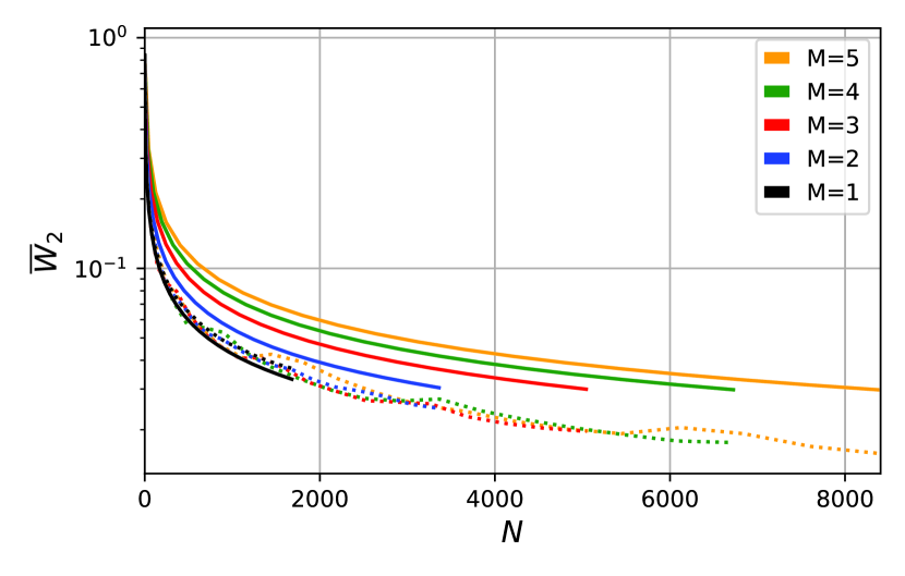
(a) Empirical estimates and formal bounds on $\overline{W}_{2}$ from grid-constrained signatures.

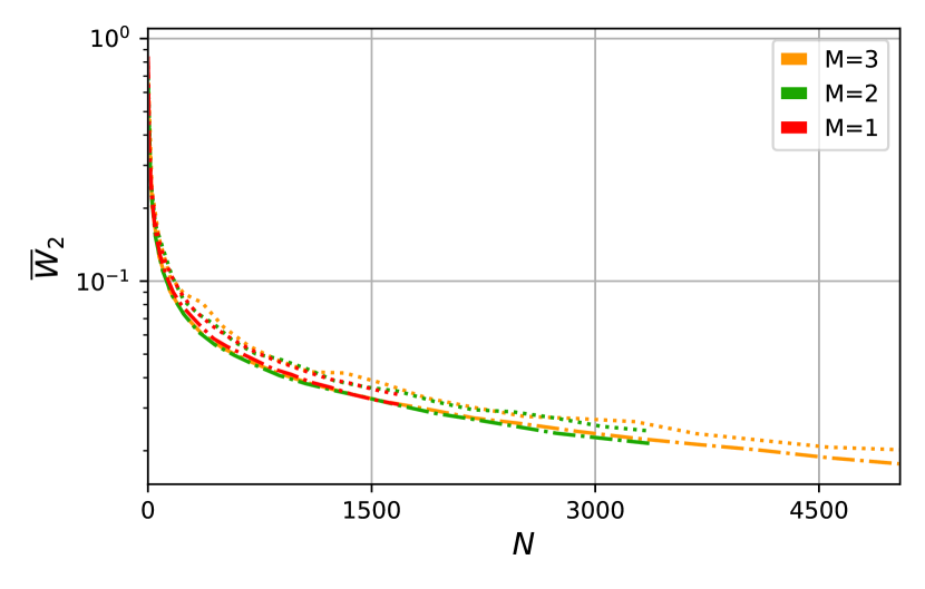
(b) Empirical estimates of $\overline{W}_{2}$ from grid-constrained and unconstrained signature locations.

Figure 9: The relative 2-Wasserstein distance between a 2D Gaussian mixture distribution with $M$ components and the signature with $N$ grid-constrained locations obtained via Algorithm 2 (solid and dotted lines), and the signature with $N$ unconstrained optimal locations (dash-dotted line). The unconstrained optimal locations are obtained by performing $N$-Means clustering on $1e3$ MC samples from the GMM. The solid lines represent the formal bounds on the relative 2-Wasserstein distance provided by Algorithm 2, while the dotted and dash-dotted lines show empirical approximations.

In this section, we experimentally evaluate the effectiveness of Algorithm 2 in constructing signatures on Gaussian mixtures. Specifically, we examine the conservatism of the formal bound on the 2-Wasserstein distance resulting from the signature operation provided by Algorithm 2, and analyze the restrictiveness of having the signature locations of each component of the mixture on a grid as in Algorithm 2.

In Figure 9(a), we analyze how the approximation error from the signature of a Gaussian mixture with $M$ components, obtained according to Algorithm 2, changes with increasing signature size. The plots show that as the signature size increases, the approximation error, measured as the relative 2-Wasserstein distance $\overline{W}_{2}$, decreases uniformly. Furthermore, in line with Corollary 10, the formal upper bound on $\overline{W}_{2}$ is exact for Gaussians ($M=1$). For Gaussian mixtures ($M>1$), the conservatism introduced by the formal bounds grows approximately linearly with increasing $M$. This is because, in Algorithm 1, we bound the Wasserstein distance resulting from the signature operation on the GMMs by the weighted sum of the 2-Wasserstein distance between each Gaussian component in the mixture and their signatures (see line 7 in Algorithm 2 and Eqn. (12)).

Recall from Subsection 5.2 that to obtain a closed-form bound on the approximation error in Algorithm 2, we place the signature locations of each component of the mixture on a grid in the transformed space induced by the element’s covariance matrix, as illustrated in Figure 4. Specifically, following Proposition 19, we choose the grids such that for a given signature size $N$, the 2-Wasserstein distance from the signature operation is minimized. In Figure 9(b), we estimate the optimality gap if we could instead place the signatures freely to minimize the 2-Wasserstein distance. Perhaps surprisingly, the plots show that placing the signatures freely only slightly reduces the 2-Wasserstein distance. Thus, although the optimal signature locations do not adhere to a grid structure (in line with literature (Graf and Luschgy, 2007)), the optimal grid approximates the optimal locations closely.

References

• Adams et al. (2023) Steven Adams, Andrea Patane, Morteza Lahijanian, and Luca Laurenti. Bnn-dp: robustness certification of bayesian neural networks via dynamic programming. In International Conference on Machine Learning, pages 133–151. PMLR, 2023.
• Adler and Taylor (2009) Robert J Adler and Jonathan E Taylor. Random fields and geometry. Springer Science & Business Media, 2009.
• Ambrogioni et al. (2018) Luca Ambrogioni, Umut Guclu, and Marcel van Gerven. Wasserstein variational gradient descent: From semi-discrete optimal transport to ensemble variational inference. arXiv preprint arXiv:1811.02827, 2018.
• Antognini (2019) Joseph M Antognini. Finite size corrections for neural network gaussian processes. arXiv preprint arXiv:1908.10030, 2019.
• Apollonio et al. (2023) Nicola Apollonio, Daniela De Canditiis, Giovanni Franzina, Paola Stolfi, and Giovanni Luca Torrisi. Normal approximation of random gaussian neural networks. arXiv preprint arXiv:2307.04486, 2023.
• Balasubramanian et al. (2024) Krishnakumar Balasubramanian, Larry Goldstein, Nathan Ross, and Adil Salim. Gaussian random field approximation via stein’s method with applications to wide random neural networks. Applied and Computational Harmonic Analysis, 72:101668, 2024.
• Basteri and Trevisan (2024) Andrea Basteri and Dario Trevisan. Quantitative gaussian approximation of randomly initialized deep neural networks. Machine Learning, pages 1–21, 2024.
• Bishop and Nasrabadi (2006) Christopher M Bishop and Nasser M Nasrabadi. Pattern recognition and machine learning, volume 4. Springer, 2006.
• Blundell et al. (2015) Charles Blundell, Julien Cornebise, Koray Kavukcuoglu, and Daan Wierstra. Weight uncertainty in neural network. In International conference on Machine Learning, pages 1613–1622. PMLR, 2015.
• Bordino et al. (2023) Alberto Bordino, Stefano Favaro, and Sandra Fortini. Non-asymptotic approximations of gaussian neural networks via second-order poincaré inequalities. arXiv preprint arXiv:2304.04010, page 3, 2023.
• Bortolussi et al. (2024) Luca Bortolussi, Ginevra Carbone, Luca Laurenti, Andrea Patane, Guido Sanguinetti, and Matthew Wicker. On the robustness of bayesian neural networks to adversarial attacks. IEEE Transactions on Neural Networks and Learning Systems, 2024.
• Bracale et al. (2021) Daniele Bracale, Stefano Favaro, Sandra Fortini, Stefano Peluchetti, et al. Large-width functional asymptotics for deep gaussian neural networks. In International Conference on Learning Representations, 2021.
• Burke et al. (2020) James V Burke, Frank E Curtis, Adrian S Lewis, Michael L Overton, and Lucas EA Simões. Gradient sampling methods for nonsmooth optimization. Numerical nonsmooth optimization: State of the art algorithms, pages 201–225, 2020.
• Cammarota et al. (2023) Valentina Cammarota, Domenico Marinucci, Michele Salvi, and Stefano Vigogna. A quantitative functional central limit theorem for shallow neural networks. Modern Stochastics: Theory and Applications, 11(1):85–108, 2023.
• Cohen et al. (2019) Jeremy Cohen, Elan Rosenfeld, and Zico Kolter. Certified adversarial robustness via randomized smoothing. In International Conference on Machine Learning, pages 1310–1320. PMLR, 2019.
• Davis et al. (2016) Timothy A Davis, Sivasankaran Rajamanickam, and Wissam M Sid-Lakhdar. A survey of direct methods for sparse linear systems. Acta Numerica, 25:383–566, 2016.
• Delon and Desolneux (2020) Julie Delon and Agnes Desolneux. A wasserstein-type distance in the space of gaussian mixture models. SIAM Journal on Imaging Sciences, 13(2):936–970, 2020.
• Duvenaud et al. (2014) David Duvenaud, Oren Rippel, Ryan Adams, and Zoubin Ghahramani. Avoiding pathologies in very deep networks. In Artificial Intelligence and Statistics, pages 202–210. PMLR, 2014.
• Dyer and Gur-Ari (2019) Ethan Dyer and Guy Gur-Ari. Asymptotics of wide networks from feynman diagrams. arXiv preprint arXiv:1909.11304, 2019.
• Eldan et al. (2021) Ronen Eldan, Dan Mikulincer, and Tselil Schramm. Non-asymptotic approximations of neural networks by gaussian processes. In Conference on Learning Theory, pages 1754–1775. PMLR, 2021.
• Favaro et al. (2023) Stefano Favaro, Boris Hanin, Domenico Marinucci, Ivan Nourdin, and Giovanni Peccati. Quantitative clts in deep neural networks. arXiv preprint arXiv:2307.06092, 2023.
• Flam-Shepherd et al. (2017) Daniel Flam-Shepherd, James Requeima, and David Duvenaud. Mapping gaussian process priors to bayesian neural networks. In NIPS Bayesian deep learning workshop, volume 3, 2017.
• Flam-Shepherd et al. (2018) Daniel Flam-Shepherd, James Requeima, and David Duvenaud. Characterizing and warping the function space of bayesian neural networks. In NeurIPS Workshop on Bayesian Deep Learning, page 18, 2018.
• Fortuin (2022) Vincent Fortuin. Priors in bayesian deep learning: A review. International Statistical Review, 90(3):563–591, 2022.
• Frankle and Carbin (2018) Jonathan Frankle and Michael Carbin. The lottery ticket hypothesis: Finding sparse, trainable neural networks. In International Conference on Learning Representations, 2018.
• Gal and Ghahramani (2016) Yarin Gal and Zoubin Ghahramani. Dropout as a bayesian approximation: Representing model uncertainty in deep learning. In international conference on machine learning, pages 1050–1059. PMLR, 2016.
• Garriga-Alonso and van der Wilk (2021) Adrià Garriga-Alonso and Mark van der Wilk. Correlated weights in infinite limits of deep convolutional neural networks. In Uncertainty in Artificial Intelligence, pages 1998–2007. PMLR, 2021.
• Garriga-Alonso et al. (2019) Adrià Garriga-Alonso, Carl Edward Rasmussen, and Laurence Aitchison. Deep convolutional networks as shallow gaussian processes. In International Conference on Learning Representations, 2019.
• Gibbs and Su (2002) Alison L Gibbs and Francis Edward Su. On choosing and bounding probability metrics. International statistical review, 70(3):419–435, 2002.
• Givens and Shortt (1984) Clark R Givens and Rae Michael Shortt. A class of wasserstein metrics for probability distributions. Michigan Mathematical Journal, 31(2):231–240, 1984.
• Goodfellow et al. (2016) Ian Goodfellow, Yoshua Bengio, Aaron Courville, and Yoshua Bengio. Deep learning, volume 1. MIT Press, 2016.
• Graf and Luschgy (2007) Siegfried Graf and Harald Luschgy. Foundations of quantization for probability distributions. Springer, 2007.
• Hanin (2023) Boris Hanin. Random neural networks in the infinite width limit as gaussian processes. The Annals of Applied Probability, 33(6A):4798–4819, 2023.
• Hazan and Jaakkola (2015) Tamir Hazan and Tommi Jaakkola. Steps toward deep kernel methods from infinite neural networks. arXiv preprint arXiv:1508.05133, 2015.
• Hernández-Lobato and Adams (2015) José Miguel Hernández-Lobato and Ryan Adams. Probabilistic backpropagation for scalable learning of bayesian neural networks. In International conference on machine learning, pages 1861–1869. PMLR, 2015.
• Hershey and Olsen (2007) John R Hershey and Peder A Olsen. Approximating the kullback leibler divergence between gaussian mixture models. In 2007 IEEE International Conference on Acoustics, Speech and Signal Processing-ICASSP’07, volume 4, pages IV–317. IEEE, 2007.
• Immer et al. (2021) Alexander Immer, Matthias Bauer, Vincent Fortuin, Gunnar Rätsch, and Khan Mohammad Emtiyaz. Scalable marginal likelihood estimation for model selection in deep learning. In International Conference on Machine Learning, pages 4563–4573. PMLR, 2021.
• Jacot et al. (2018) Arthur Jacot, Franck Gabriel, and Clément Hongler. Neural tangent kernel: Convergence and generalization in neural networks. Advances in neural information processing systems, 31, 2018.
• Kasim (2020) Muhammad Firmansyah Kasim. Derivatives of partial eigendecomposition of a real symmetric matrix for degenerate cases. arXiv preprint arXiv:2011.04366, 2020.
• Khan et al. (2018) Mohammad Khan, Didrik Nielsen, Voot Tangkaratt, Wu Lin, Yarin Gal, and Akash Srivastava. Fast and scalable bayesian deep learning by weight-perturbation in adam. In International Conference on Machine Learning, pages 2611–2620. PMLR, 2018.
• Khan et al. (2019) Mohammad Emtiyaz E Khan, Alexander Immer, Ehsan Abedi, and Maciej Korzepa. Approximate inference turns deep networks into gaussian processes. Advances in neural information processing systems, 32, 2019.
• Kieffer (1982) J Kieffer. Exponential rate of convergence for lloyd’s method i. IEEE Transactions on Information Theory, 28(2):205–210, 1982.
• Kingma and Ba (2014) Diederik P Kingma and Jimmy Ba. Adam: A method for stochastic optimization. arXiv preprint arXiv:1412.6980, 2014.
• Klukowski (2022) Adam Klukowski. Rate of convergence of polynomial networks to gaussian processes. In Conference on Learning Theory, pages 701–722. PMLR, 2022.
• Krizhevsky et al. (2012) Alex Krizhevsky, Ilya Sutskever, and Geoffrey E Hinton. Imagenet classification with deep convolutional neural networks. In Advances in Neural Information Processing Systems 25, pages 1097–1105. Curran Associates, Inc., 2012.
• Lee et al. (2017) Jaehoon Lee, Yasaman Bahri, Roman Novak, Samuel S Schoenholz, Jeffrey Pennington, and Jascha Sohl-Dickstein. Deep neural networks as gaussian processes. arXiv preprint arXiv:1711.00165, 2017.
• Lee et al. (2020) Jaehoon Lee, Samuel Schoenholz, Jeffrey Pennington, Ben Adlam, Lechao Xiao, Roman Novak, and Jascha Sohl-Dickstein. Finite versus infinite neural networks: an empirical study. Advances in Neural Information Processing Systems, 33:15156–15172, 2020.
• Liu and Wang (2016) Qiang Liu and Dilin Wang. Stein variational gradient descent: A general purpose bayesian inference algorithm. Advances in neural information processing systems, 29, 2016.
• Lloyd (1982) Stuart Lloyd. Least squares quantization in pcm. IEEE transactions on information theory, 28(2):129–137, 1982.
• Louizos et al. (2017) Christos Louizos, Karen Ullrich, and Max Welling. Bayesian compression for deep learning. Advances in neural information processing systems, 30, 2017.
• MacKay (1996) David JC MacKay. Bayesian non-linear modeling for the prediction competition. In Maximum Entropy and Bayesian Methods: Santa Barbara, California, USA, 1993, pages 221–234. Springer, 1996.
• Magnus and Neudecker (2019) Jan R Magnus and Heinz Neudecker. Matrix differential calculus with applications in statistics and econometrics. John Wiley & Sons, 2019.
• Mäkelä (2002) Marko Mäkelä. Survey of bundle methods for nonsmooth optimization. Optimization methods and software, 17(1):1–29, 2002.
• Matsubara et al. (2021) Takuo Matsubara, Chris J Oates, and François-Xavier Briol. The ridgelet prior: A covariance function approach to prior specification for bayesian neural networks. The Journal of Machine Learning Research, 22(1):7045–7101, 2021.
• Matthews et al. (2018) Alexander G de G Matthews, Mark Rowland, Jiri Hron, Richard E Turner, and Zoubin Ghahramani. Gaussian process behaviour in wide deep neural networks. arXiv preprint arXiv:1804.11271, 2018.
• McLachlan and Peel (2000) Geoffrey J McLachlan and David Peel. Finite mixture models, volume 299. John Wiley & Sons, 2000.
• Mnih et al. (2013) Volodymyr Mnih, Koray Kavukcuoglu, David Silver, Alex Graves, Ioannis Antonoglou, Daan Wierstra, and Martin Riedmiller. Playing atari with deep reinforcement learning. arXiv preprint arXiv:1312.5602, 2013.
• Neal (2012) Radford M Neal. Bayesian learning for neural networks, volume 118. Springer Science & Business Media, 2012.
• Novak et al. (2018) Roman Novak, Lechao Xiao, Yasaman Bahri, Jaehoon Lee, Greg Yang, Jiri Hron, Daniel A Abolafia, Jeffrey Pennington, and Jascha Sohl-dickstein. Bayesian deep convolutional networks with many channels are gaussian processes. In International Conference on Learning Representations, 2018.
• Pagès and Printems (2003) Gilles Pagès and Jacques Printems. Optimal quadratic quantization for numerics: the gaussian case. Monte Carlo Methods Appl., 9(2):135–165, 2003.
• Pages and Wilbertz (2012) Gilles Pages and Benedikt Wilbertz. Optimal delaunay and voronoi quantization schemes for pricing american style options. In Numerical Methods in Finance: Bordeaux, June 2010, pages 171–213. Springer, 2012.
• Peyré et al. (2019) Gabriel Peyré, Marco Cuturi, et al. Computational optimal transport: With applications to data science. Foundations and Trends® in Machine Learning, 11(5-6):355–607, 2019.
• Rasmussen (2003) Carl Edward Rasmussen. Gaussian processes in machine learning. In Summer school on machine learning, pages 63–71. Springer, 2003.
• Rockafellar (2015) R. Tyrrell Rockafellar. Convex Analysis. Princeton Landmarks in Mathematics and Physics. Princeton University Press, Princeton, NJ, revised edition edition, 2015. ISBN 978-0691015866.
• Schoenholz et al. (2016) Samuel S Schoenholz, Justin Gilmer, Surya Ganguli, and Jascha Sohl-Dickstein. Deep information propagation. In International Conference on Learning Representations, 2016.
• Simonyan and Zisserman (2014) Karen Simonyan and Andrew Zisserman. Very deep convolutional networks for large-scale image recognition. arXiv preprint arXiv:1409.1556, 2014.
• Srivastava et al. (2014) Nitish Srivastava, Geoffrey Hinton, Alex Krizhevsky, Ilya Sutskever, and Ruslan Salakhutdinov. Dropout: a simple way to prevent neural networks from overfitting. The journal of machine learning research, 15(1):1929–1958, 2014.
• Szegedy et al. (2013) Christian Szegedy, Wojciech Zaremba, Ilya Sutskever, Joan Bruna, Dumitru Erhan, Ian Goodfellow, and Rob Fergus. Intriguing properties of neural networks. arXiv preprint arXiv:1312.6199, 2013.
• Tang and Salakhutdinov (2013) Charlie Tang and Russ R Salakhutdinov. Learning stochastic feedforward neural networks. Advances in Neural Information Processing Systems, 26, 2013.
• Tran et al. (2022) Ba-Hien Tran, Simone Rossi, Dimitrios Milios, and Maurizio Filippone. All you need is a good functional prior for bayesian deep learning. Journal of Machine Learning Research, 23(74):1–56, 2022.
• Tresp (2000) Volker Tresp. Mixtures of gaussian processes. Advances in neural information processing systems, 13, 2000.
• Van Amersfoort et al. (2020) Joost Van Amersfoort, Lewis Smith, Yee Whye Teh, and Yarin Gal. Uncertainty estimation using a single deep deterministic neural network. In International conference on machine learning, pages 9690–9700. PMLR, 2020.
• Villani et al. (2009) Cédric Villani et al. Optimal transport: old and new, volume 338. Springer, 2009.
• Wicker et al. (2020) Matthew Wicker, Luca Laurenti, Andrea Patanè, and Marta Kwiatkowska. Probabilistic safety for Bayesian neural networks. Uncertainty in Artificial Intelligence (UAI), 2020.
• Wilhelm et al. (2012) Stefan Wilhelm et al. Moments calculation for the doubly truncated multivariate normal density. arXiv preprint arXiv:1206.5387, 2012.
• Williams (1996) Christopher Williams. Computing with infinite networks. Advances in neural information processing systems, 9, 1996.
• Yaida (2020) Sho Yaida. Non-gaussian processes and neural networks at finite widths. In Mathematical and Scientific Machine Learning, pages 165–192. PMLR, 2020.
• Yu et al. (2021) Tianyuan Yu, Yongxin Yang, Da Li, Timothy Hospedales, and Tao Xiang. Simple and effective stochastic neural networks. In Proceedings of the AAAI Conference on Artificial Intelligence, volume 35, pages 3252–3260, 2021.
• Zhang et al. (2018) Guodong Zhang, Shengyang Sun, David Duvenaud, and Roger Grosse. Noisy natural gradient as variational inference. In International Conference on Machine Learning, pages 5852–5861. PMLR, 2018.