Absorbing discretisation effects with a massive renormalization scheme: the charm-quark mass

Abstract

We present the first numerical implementation of the massive SMOM ($\mathrm{mSMOM}$) renormalization scheme and use it to calculate the charm quark mass. Based on ensembles with three flavours of dynamical domain wall fermions with lattice spacings in the range $0.11$ – $0.08\,\mathrm{fm}$, we demonstrate that the mass scale which defines the $\mathrm{mSMOM}$ scheme can be chosen such that the extrapolation has significantly smaller discretisation effects than the $\mathrm{SMOM}$ scheme. Converting our results to the $\overline{\mathrm{MS}}$ scheme we obtain $\overline{m}_{c}(3\,\mathrm{GeV})=1.008(13)\,\mathrm{GeV}$ and $\overline{m}_{c}(\overline{m}_{c})=1.292(12)\,\mathrm{GeV}$.

I Introduction

Non-perturbative massive renormalization schemes, such as the ones introduced in Ref. Boyle et al. (2017a), yield renormalized correlators that satisfy vector and axial Ward identities independently of the value of the quark masses and are expected to reabsorb some of the lattice artefacts that come in powers of $am$ and can be large for heavy quark masses. These schemes are therefore interesting candidates to renormalize quantities that are affected by large cut-off effects, leading to milder extrapolations to the continuum limit compared to the usual massless schemes that are currently used.

In this paper, we present the first numerical implementation of the renormalization conditions that were spelled out in Ref. Boyle et al. (2017a) and extract the renormalization constants that are needed in order to compute the renormalized charm-quark mass in these massive symmetric-momentum-subtraction (mSMOM) schemes. The schemes are labelled by the momentum scale of the subtraction point and by the value of the renormalized quark mass at which the renormalization conditions are imposed. Lattice artefacts depend on the choice of this mass, which can be tuned in order to obtain flatter extrapolations. We use lattice QCD ensembles generated by the RBC/UKQCD collaboration, with 2+1 dynamical flavours and inverse lattice spacings ranging from $a^{-1}=1.73~{}\mathrm{GeV}$ to $2.79~{}\mathrm{GeV}$. We compute all the lattice correlators that enter the renormalization conditions and spell out in detail the workflow to implement and solve the correct set of equations.

Results in different mSMOM schemes are converted to ${\overline{\text{MS}}}$ using one-loop conversion factors and show a pleasing consistency. The main result of this first study confirms the theoretical expectation motivating massive schemes. They provide a (simple) way to absorb some of the mass-dependent lattice artefacts and yield more reliable extrapolations to the continuum limit.

The remainder of this paper is organised as follows. In Section II we remind the reader of the details of the massive non-perturbative renormalization scheme. In Section III we provide details of our numerical set-up before presenting the details of our analysis and our final results in Section IV. We conclude with an outlook in section V. An early stage of this analysis was reported in Ref. Del Debbio et al. (2023)

II Massive NPR

Before discussing the numerical analysis that was performed for this paper, we summarise the main ideas behind massive renormalization schemes. To keep our presentation self-contained, we quote below the renormalization conditions defining $\mathrm{mSMOM}$ schemes, which were originally spelled out in Ref. Boyle et al. (2017a). To match the numerical simulations, we work in Euclidean space. In our conventions, bare quantities are written without any suffix, while their renormalized counterparts are identified by a suffix $R$. The renormalization conditions are usually expressed in terms of amputated correlators of fermion bilinears

$$\Lambda^{a}_{\Gamma}(p_{2},p_{3})=S(p_{3})^{-1}G^{a}_{\Gamma}(p_{3},p_{2})S(p_{2})^{-1}\,,$$ (1)

where $S(p)$ is the fermion propagator,

$$S(p)=\int d^{4}x\,e^{-ip\cdot x}\langle\psi(x)\bar{\psi}(0)\rangle\,,$$ (2)

and $G^{a}_{\Gamma}(p_{3},p_{2})=\langle O^{a}_{\Gamma}(q)\bar{\psi}(p_{3})\psi(p_{2})\rangle$ with $O^{a}_{\Gamma}=\bar{\psi}\Gamma\tau^{a}\psi$. The superscript $a$, which will be dropped henceforth, denotes that we consider flavour non-singlet bilinears, with $\tau^{a}$ a generic flavour-rotation generator. In the following we will also suppress the superscript $\mathrm{mSMOM}$ unless it is required to avoid ambiguity.

We choose the same symmetric momentum configurations as those chosen in in the massless $\mathrm{SMOM}$ scheme, i.e. $q^{2}\equiv(p_{2}-p_{3})^{2}=p_{2}^{2}=p_{3}^{3}=\mu^{2}$, where $\mu$ is the renormalization scale. The massive scheme requires the introduction of another scale, $\overline{m}_{R}$, a renormalized mass at which the renormalization conditions are imposed. The massless scheme is recovered in the limit $\overline{m}_{R}\to 0$. For the $\mathrm{mSMOM}$ scheme in Euclidean space the renormalization conditions, to be evaluated with the symmetric momentum configuration imposed and at $m_{R}=\overline{m}_{R}$, read

$$1 =\frac{1}{12p^{2}}\operatorname{Tr}\left[-iS_{R}(p)^{-1}\cancel{p}\right],$$ (3)

$$1 =\frac{1}{12m_{R}}\Big{\{}\operatorname{Tr}\left[S_{R}(p)^{-1}\right]+\frac{1}{2}\operatorname{Tr}\left[\left(iq\cdot\Lambda_{\mathrm{A},R}\right)\gamma_{5}\right]\Big{\}},$$ (4)

$$1 =\frac{1}{12q^{2}}\operatorname{Tr}\left[\left(q\cdot\Lambda_{\mathrm{V},R}\right)\cancel{q}\right],$$ (5)

$$1 =\frac{1}{12q^{2}}\operatorname{Tr}\left[\left(q\cdot\Lambda_{\mathrm{A},R}\,+\,2m_{R}\Lambda_{\mathrm{P},R}\right)\gamma_{5}\cancel{q}\right],$$ (6)

$$1 =\frac{1}{12i}\operatorname{Tr}\left[\Lambda_{\mathrm{P},R}\gamma_{5}\right],$$ (7)

$$1 =\frac{1}{12}\operatorname{Tr}\left[\Lambda_{\mathrm{S},R}\right]+\,\frac{1}{6q^{2}}\operatorname{Tr}\left[2m_{R}\Lambda_{\mathrm{P},R}\gamma_{5}\cancel{q}\right].$$ (8)

The renormalized quantities are defined as follows:

$$\psi_{R}=Z_{q}^{1/2}\psi\,,\quad m_{R}=Z_{m}m\,,\quad O_{\Gamma,R}=Z_{\Gamma}O_{\Gamma}\,,$$ (9)

where $m$ denotes a quark mass. The renormalized propagator and amputated vertex functions are

$$S_{R}(p)=Z_{q}S(p)\,,\quad\Lambda_{\Gamma,R}(p_{2},p_{3})=\frac{Z_{\Gamma}}{Z_{q}}\Lambda_{\Gamma}(p_{2},p_{3})\,.$$ (10)

As discussed in the original publication Boyle et al. (2017a), these conditions ensure that renormalized correlators satisfy the Ward identities of the continuum theory, which in turn lead to useful constraints on the renormalization constants, namely

$$Z_{\mathrm{V}}=Z_{\mathrm{A}}=1,\quad Z_{\mathrm{P}}=Z_{\mathrm{S}},\quad Z_{m}Z_{\mathrm{P}}=1\,.$$ (11)

Substituting Eqs. (9) and (10) into the renormalization conditions Eqs. (3)–(8) and solving the system of equations gives access to the renormalization factors $Z_{q}$, $Z_{m}$, $Z_{A}$, $Z_{V}$, $Z_{S}$ and $Z_{P}$. In practice we find it convenient to replace the renormalization condition Eq. (3) by a direct determination of $Z_{A}$ from ratios of conserved and local axial currents. Combined with Eqs. (4)–(8) this still gives access to all the required renormalization constants.

Note that by construction the renormalization constants in a massive scheme depend on both the coupling and the dimensionless product $a\overline{m}$. The $\mathrm{mSMOM}$ schemes are defined by tuning the renormalized quark mass to some arbitrary scale $\overline{m}_{R}$, where the renormalization conditions need to be satisfied.

The arbitrariness in the choice of $\overline{m}_{R}$ can be turned into a useful tool when extrapolating lattice QCD results to the continuum limit. Indeed, the ideal choice of $\overline{m}_{R}$ is determined by requiring that the observables of interest have a mild dependence on the lattice spacing in that particular scheme. Different observables may dictate different values of $\overline{m}_{R}$; this is not a problem, since we know how to connect schemes corresponding to different choices of $\overline{m}_{R}$ to a common reference scheme such as, e.g., $\overline{\mathrm{MS}}$, using the one-loop perturbative expressions in Ref. Boyle et al. (2017a) and in Appendix B.

The focus of this paper is to compute the renormalized charm-quark mass in $\mathrm{mSMOM}$, which is defined as

$$m^{\mathrm{mSMOM}}_{c,R}(\mu,\overline{m}_{R})=\lim_{a\to 0}Z_{m}^{\mathrm{mSMOM}}(g,a\mu,a\overline{m})(am_{c})a^{-1}\,,\\$$ (12)

where the mass scale $\overline{m}_{R}$ defining the renormalization scheme is obtained through

$$\overline{m}_{R}(\mu,\overline{m}_{R})=\lim_{a\to 0}Z_{m}^{\mathrm{mSMOM}}(g,a\mu,a\overline{m})(a\overline{m})a^{-1}\,,$$ (13)

and the bare quark mass in lattice units ($am$) is the sum of the input quark mass $am_{q}$ and the additive mass renormalization $am_{\mathrm{res}}$

$$am\equiv\left(am_{q}+am_{\mathrm{res}}\right)\,,$$ (14)

$Z_{m}^{\mathrm{mSMOM}}(g,a\mu,a\overline{m}_{R})$ is the renormalization constant defined by the renormalization conditions above and the bare mass of the charm quark is set by requiring that the mass of the heavy-heavy pseudoscalar meson coincides with the mass of the physical $\eta_{c}$ meson.

After taking the continuum limit, the mSMOM renormalized mass can be converted to ${\overline{\text{MS}}}$,

$$m_{R}^{\overline{\text{MS}}}(\tilde{\mu})=R^{{\overline{\text{MS}}}\leftarrow\text{mSMOM}}(\tilde{\mu},\mu,{\overline{m}}_{R})m_{R}^{\text{mSMOM}}(\mu,{\overline{m}}_{R}),$$ (15)

where the dimensionful scale $\tilde{\mu}$ stems from dimensional regularisation and will in practice be set equal to $\mu$. The conversion factor $R^{{\overline{\text{MS}}}\leftarrow\text{mSMOM}}=Z_{m}^{\overline{\text{MS}}}/Z^{\text{mSMOM}}_{m}$ is evaluated at one-loop in perturbation theory in Appendix B.

III Simulation set up and strategy

Table 1: Summary of the main parameters of the ensembles used in this work. In the ensemble name the first letter (C, M or F) stands for coarse, medium and fine, respectively. The last letter (M or S) stands for Möbius and Shamir kernels, respectively.

name	$L/a$	$T/a$	$a^{-1}[\textrm{GeV}]$	$M_{\pi}[\textrm{MeV}]$	$am_{l}$	$am_{s}$
C1M	$24$	$64$	1.7295(38)	276	0.005	0.0362
C1S	$24$	$64$	1.7848(50)	340	0.005	0.04
M0M	$64$	$128$	2.3586(70)	139	0.000678	0.02661
M1M	$32$	$64$	2.3586(70)	286	0.004	0.02661
M1S	$32$	$64$	2.3833(86)	304	0.004	0.03
F1M	$48$	$96$	2.708(10)	232	0.002144	0.02144
F1S	$48$	$96$	2.785(11)	267	0.002144	0.02144

Table 2: Heavier input quark masses that were simulated in addition to $am_{l}$, $2am_{l}$, $am_{s}/2$ and $am_{s}$.

ens	$am_{q}$
C1M	0.05, 0.1, 0.15, 0.2, 0.3
C1S	0.05, 0.1, 0.15, 0.2, 0.3, 0.33
M1M	0.05, 0.1, 0.15, 0.225, 0.3, 0.32, 0.34
M1S	0.05, 0.1, 0.15, 0.225, 0.3, 0.32, 0.34, 0.36, 0.375
F1M	0.033, 0.066, 0.099, 0.132, 0.198, 0.264, 0.33, 0.36
F1S	0.033, 0.066, 0.099, 0.132, 0.198, 0.264, 0.33, 0.36, 0.396

We use RBC/UKQCD’s ensembles Aoki et al. (2011); Blum et al. (2016); Boyle et al. (2017b, 2018, 2024) with Iwasaki gauge action Iwasaki and Yoshie (1984); Iwasaki (1985) and domain-wall fermion action Shamir (1993); Furman and Shamir (1995). They include the dynamical effects from degenerate up and down quarks as well as the strange quark. The main ensemble properties are listed in Table 1. For each of the three lattice spacings we have one ensemble with the Shamir domain-wall kernel Shamir (1993) (last letter ‘S’) and one with the Möbius domain-wall kernel Brower et al. (2005, 2006, 2017) (last letter ‘M’). The parameters of these kernels are chosen such that a combined continuum limit with all ensembles is possible Blum et al. (2016). In addition we have data around the physical charm quark mass on the physical pion mass ensemble M0M which differs from M1M only in pion mass and volume.

We implement the SMOM momentum configuration by choosing momenta $p_{2}=(p,p,0,0)$ and $p_{3}=(p,0,p,0)$ where $p=\frac{2\pi}{L}(n+\theta)$. Since our aim is to comprehensively cover the region $2\,\mathrm{GeV}\lesssim q\lesssim 3\,\mathrm{GeV}$ we use twist angles $\theta\in\{0,0.25,0.5,0.75\}$ in combination with Fourier modes $n\in\{3,4,5\}$ for the coarse and medium, and $n\in\{4,5,6\}$ for the fine ensembles.

We map out the parameter space by simulating at several quark masses $am_{q}$ between the light-quark mass and the largest quark mass we can reach on a given ensemble whilst maintaining good control over the residual-mass determination and the domain-wall formalism Boyle et al. (2016a). Since we expect sea-pion mass and finite volume effects to be negligible for the determination of the charm quark mass, the main numerical analysis is based on the computationally cheaper non-physical pion mass ensembles. However, in order to assess these effects, we simulated a small number of heavy quark masses in the charm region on the M0M ensemble which can be directly compared with the equivalent M1M datapoints. As we will see in Sec. IV.1 sea-pion mass effects are at the sub-permille level.

The chosen quark masses are listed in Table 2. The measurements were carried out using the Grid and Hadrons libraries Boyle et al. (2016b); Yamaguchi et al. (2022); Portelli et al. (2023).

For each input quark mass $am_{q}$ we compute vertex functions (see Eq. (1)) as well as several mesonic flavour-diagonal quark-connected two-point correlation functions. For the latter we use a mild Jacobi smearing to improve the overlap with the ground state for heavy masses, in particular for the pseudoscalar density $P$, the midpoint pseudoscalar density $J_{5q}$ Furman and Shamir (1995) and the local ($L$) and conserved ($C$) Blum et al. (2004); Boyle (2014); Blum et al. (2016) versions of the temporal component of the axial current. We determine the residual mass $am_{\mathrm{res}}$ and the renormalization constant $Z_{A}$ from the late time behaviour of ratios of these correlation functions via

$$am_{\mathrm{res}}^{\mathrm{eff}}(t)=\frac{\left<PJ_{5q}\right>(t)}{\left<PP\right>(t)}\,,$$ (16)

and

$$Z_{A}^{\mathrm{eff}}(t)=\frac{1}{2}\left[\frac{C(t+\frac{1}{2})+C(t-\frac{1}{2})}{2L(t)}+\frac{2C(t+\frac{1}{2})}{L(t)+L(t+1)}\right]\,.$$ (17)

Throughout this work we set the quark mass using the quark-connected flavour-diagonal pseudoscalar meson $M_{\eta_{h}}$, since the quantity we are ultimately interested in is the charm quark mass and the contribution from quark-disconnected pieces to the mass of the $\eta_{c}$ meson has been estimated to be negligibly small Davies et al. (2010). We explore reference masses in the range $\frac{1}{2}M^{\mathrm{PDG}}_{\eta_{c}}$ to $M^{\mathrm{PDG}}_{\eta_{c}}=2.9839(4)\,\mathrm{GeV}$ Workman et al. (2022).

The strategy of our calculation is as follows:

1. For each mass $am_{q}$ on each ensemble, determine $am_{\mathrm{res}}$ and hence $am$ as well as $aM_{\eta_{h}}(am)$, $Z_{A}(g,am)$, $Z_{m}(g,a\mu,am)$.

2. Interpolate $Z_{m}(g,a\mu,am)$ to a common momentum scale $\hat{\mu}$ to obtain $Z_{m}(g,a\hat{\mu},am)$ on all ensembles.

3. Fix two mass-scales: the scale $\overline{m}$ at which the renormalization conditions are imposed and the quark mass $m$ to be determined. These do not have to be the same.

   In practice we define a set of meson masses $M_{i}$ such that $M_{i}/M_{\eta_{c}}^{\mathrm{PDG}}\in\{0.5,0.6,0.7,0.75,0.8,0.9,1\}$. We interpolate $am(aM)$ to each choice of $M_{i}$ to obtain $am_{i}$ and similarly interpolate $Z_{m}(g,a\hat{\mu},am)$ to obtain $Z_{m}(g,a\hat{\mu},am_{i})$. We note that the heaviest two and three values of $M_{i}$ are not directly accessible on the C1S and C1M ensembles, respectively.

   Then, we define the mass-scale $\overline{m}$ of the renormalization condition by fixing a meson mass $\overline{M}$ to be one of the $M_{i}$ and set the bare quark mass $m$ by fixing a meson mass $M$ to a potentially different $M_{i}$.

4. For the given choice of $M$ and $\overline{M}$, combine $Z_{m}(g,a\hat{\mu},a\overline{m})$ and $am$ to obtain the right hand side of Eq. (12) on each ensemble. Take the continuum limit to obtain $m_{R}(\hat{\mu},\overline{m}_{R})$. Finally, (since $M$ and $\overline{M}$ can differ) also take the continuum limit to obtain $\overline{m}_{R}(\hat{\mu},\overline{m}_{R})$ (c.f. Eq. (13)). This last step is required in order to know the mass scale of the renormalization condition which is needed to relate it to other schemes such as $\mathrm{SMOM}$ or $\overline{\mathrm{MS}}$.

5. Our choice of domain wall parameters does not allow for direct simulations at the physical charm quark mass on the coarse lattice spacing. Hence we repeat this procedure for different values of $M$, but at fixed $\overline{M}$. This yields values $m_{i,R}^{\mathrm{mSMOM}}(\hat{\mu},\overline{m}_{R})$ as a function of $M_{i}$, which can be parameterised to finally obtain the value of $m_{c,R}^{\mathrm{mSMOM}}(\hat{\mu},\overline{m}_{R})$.

6. Finally, repeat the entire analysis for different choices of $\hat{\mu}$ and $\overline{M}$ in order to determine the ideal choice of $\overline{m}$ for a given $\hat{\mu}$.

IV Results

In this section we carry out the analysis outlined above.

IV.1 From correlators to observables

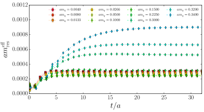
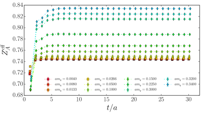
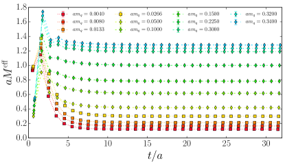
Figure 1: Representative effective $am_{\mathrm{res}}$ (top) and $Z_{A}$ (middle) and $aM_{\eta_{h}}$ (bottom)values on the M1M ensemble.

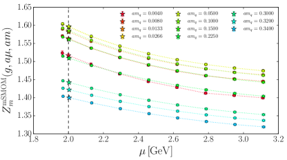
Figure 2: Interpolation of $Z_{m}$ to a scale of $\mu=2\,\mathrm{GeV}$ for various input quark mass $am_{q}$. The stars indicate the value of $Z_{m}^{\mathrm{mSMOM}}$ interpolated to $\hat{\mu}=2\,\mathrm{GeV}$.

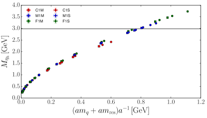
Figure 3: Coverage of the quark mass dependence of our data.

We first determine $am_{\mathrm{res}}$, $Z_{A}$ and $aM$ on all ensembles and for each choice of quark mass. The plots in Figure 1 illustrate the time behaviour of the data on the M1M ensemble (c.f. Eqs (16) and (17)) from which these quantities can be determined at late times. As expected from our previous work Boyle et al. (2016a), we find that for large quark masses, the residual mass grows and eventually becomes unbounded. We conservatively discard any data where this might be the case and only show data points for which the residual mass reaches a plateau at late times. We observe stable plateaus for all data points that are included in the analysis. Since the data is very precise and the plateaus are unambiguous, we do not perform fits to the data, but simply take the midpoint value (rightmost points in the plots in Figure 1). Numerical values for all data points are presented in Tables 5-10 in Appendix A. Figure 3 shows the spectrum as a function of the bare quark mass $m$. Combining the determination of $Z_{A}$ for each simulated mass point with the system of equations Eqs. (4)-(8) we obtain the corresponding values of $Z^{\mathrm{mSMOM}}_{m}$ at each mass point for the simulated renormalization scales $\mu$.

Table 3: Comparison of observables between the M0M ($M_{\pi}=139\,\mathrm{MeV}$) and the M1M ($M_{\pi}=286\,\mathrm{MeV}$) ensembles for two mass points bracketing the physical charm quark mass.

0.32	M0M	M1M	M0M/M1M
$aM$	1.23636(19)	1.23593(61)	1.00035(53)
$am_{\mathrm{res}}$	0.0006613(18)	0.0006617(21)	0.9993(41)
$Z_{A}$	0.824110(43)	0.824154(95)	0.99995(12)
0.34	M0M	M1M	M0M/M1M
$aM$	1.28092(18)	1.28049(61)	1.00033(50)
$am_{\mathrm{res}}$	0.0009049(26)	0.0009004(28)	1.0050(43)
$Z_{A}$	0.833863(42)	0.833897(100)	0.99996(13)

Before performing the required interpolations and continuum extrapolations, we consider the size of potential effects afflicting simulations which do not take place at the physical pion mass. Table  3 contrasts the values for $aM$, $am_{\mathrm{res}}$ and $Z_{A}$ on the M0M and the M1M ensembles for two choices of the heavy quark mass that bracket the physical charm quark mass. These two ensembles only differ in their volume and pion mass. We observe that the respective values on M0M and M1M are compatible with each other and hence their ratios are compatible with unity. We further observe that the relative (albeit not statistically resolved) effect on the hadron mass is at the sub-permille level. We therefore conclude that any chiral effects in the data can be safely neglected.

IV.2 Interpolations

Having obtained $Z^{\mathrm{mSMOM}}_{m}(g,a\mu,am)$, $M(am)$ and $am$ at each simulated mass point, we now perform the interpolations listed in steps (b) and (c). Given the broad range covered by our data (cf. Figs  2 and 3), we perform these interpolations locally as polynomial fits to the closest data points. In order to estimate any systematic uncertainties stemming from these interpolations we perform them in multiple ways:

• linear interpolation between the two closest bracketing datapoints.

• quadratic interpolations between the two data points which bracket the target value and the nearest other data point to the left (right).

• a cubic interpolation between the closest 4 points.

We take the quadratic interpolation with the third data point closest to the target value as our central value and in addition to its statistical uncertainty assign half the spread between these values as a systematic uncertainty. Figure 2 illustrates this for step (b), i.e. the interpolation of $Z_{m}$ at fixed mass ($am_{q}=0.15$) to the scale of $\mu=2\,\mathrm{GeV}$). Since we want to contrast the approach to the continuum limit between the massless ($\mathrm{SMOM}$) and the massive ($\mathrm{mSMOM}$) scheme, we also compute $Z_{m}^{\mathrm{SMOM}}$.

For completeness, we list the numerical values for $Z^{\mathrm{mSMOM}}_{m}$ and $Z_{m}^{\mathrm{SMOM}}$ at $\mu=2\,\mathrm{GeV}$ in Tables 5-10. We compute $Z_{m}^{\mathrm{SMOM}}$ only in the light and strange sector and use these values to extrapolate $Z_{m}^{\mathrm{SMOM}}$ to the massless limit, prior to applying it.

IV.3 Continuum extrapolations

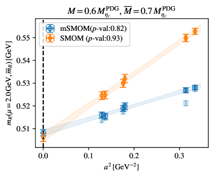
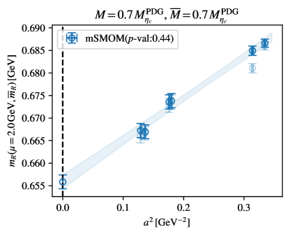
Figure 4: Top: Example continuum limit extrapolation comparing the approach to the continuum for the SMOM scheme to the that of the mSMOM scheme. The quark masses $m_{R}$ (that is being extrapolated) and $\overline{m}_{R}$ (defining the $\mathrm{mSMOM}$ scheme) are chosen to reproduce mesons of mass $0.6\times M_{\eta_{c}}^{\mathrm{PDG}}$ and $0.7\times M_{\eta_{c}}^{\mathrm{PDG}}$, respectively. Bottom: Continuum limit determining the renormalization mass scale $\overline{m}_{R}$ at which the renormalization conditions are imposed.

Having determined $am$, $a\overline{m}$ and $Z_{m}(g,a\hat{\mu},a\overline{m})$ on each ensemble, we can now perform the continuum limit of the renormalized quark mass $am$ using the $\mathrm{mSMOM}$ scheme at a renormalization scale $\hat{\mu}$ and mass scale $\overline{m}$. The most general ansatz that we consider for our continuum extrapolations is given by

$$m^{X}(a\Lambda,a\hat{\mu})=m^{X}(\hat{\mu})+C_{\chi}am_{\mathrm{res}}+C_{1}(a\Lambda)^{2}\,,$$ (18)

where the coefficient $C_{\chi}$ captures scaling violations stemming from the residual chiral symmetry breaking in our data. We tried adding a term proportional to $a^{4}$ but in practice we find that the term proportional to $a^{4}$ is compatible with zero and not needed to describe the data and we hence do not include it in the ansatz. Contrary to this, the coefficient $C_{\chi}$ is typically resolved from zero and tends to be of $O(1)$. However, the size of $am_{\mathrm{res}}$ is typically small (c.f. Tables 5-10).

We present an example continuum limit fit in the top panel of Figure 4 for the choice $\overline{M}=0.7\times M_{\eta_{c}}^{\mathrm{PDG}}$ and $M=0.6\times M_{\eta_{c}}^{\mathrm{PDG}}$. In addition to the $\mathrm{mSMOM}$ data points (blue circles) we also show the approach to the continuum limit using the chirally extrapolated value of $Z_{m}$ in the $\mathrm{SMOM}$ scheme (orange diamonds). We clearly see that the data has smaller discretisation effects in the $\mathrm{mSMOM}$ scheme than the $\mathrm{SMOM}$ scheme. The continuum extrapolated values are not expected to agree with each other, since they are not converted to the same scheme yet. However, when evaluating the conversion factors for the scale and mass at hand (compare the right hand panel of Fig 10 in Appendix B), we find the conversion factor to be very close to unity. In order to determine the exact parameters of the scheme it remains to determine the value of $\overline{m}$, i.e. to take the continuum limit where $M=\overline{M}$. This is shown for the value $0.7\times M_{\eta_{c}}^{\mathrm{PDG}}$ in the bottom panel of Figure 4.

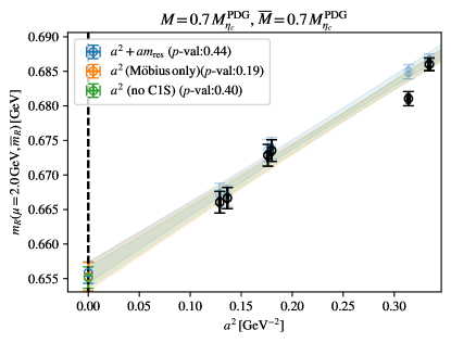
Figure 5: Variations of the continuum limit extrapolation presented in the top panel of Fig. 4

In both plots, the original $\mathrm{mSMOM}$ data points are shown as partially transparent blue symbols, the opaque blue symbols present the value once the residual mass contribution is corrected for. We notice that this only significantly affects the C1S data point, which is expected since residual chiral symmetry breaking effects are known to decrease as the lattice spacing is reduced and when increasing the Möbius scale which is one for the Shamir kernel and two for the Möbius kernel we are using. In addition, the residual mass is known to increase as the input quark mass $am_{q}$ increases as can be seen e.g. in the top panel of Fig 1.

In order to assess the systematic uncertainties associated to the continuum limit extrapolation we repeat the fit for several variations. In particular Figure 5 shows this for the case of the combination of masses $(M,\overline{M})$ presented in the top panel of Fig. 4. We consider

• fitting all ensembles on which the hadron mass $M$ can be simulated including the terms proportional to $am_{\mathrm{res}}$ and $(a\Lambda)^{2}$

• fitting all except the C1S ensemble (which has by far the largest $am_{\mathrm{res}}$ value) only including the term proportional to $(a\Lambda)^{2}$

• fitting only the Möbius ensembles (which have smaller $am_{\mathrm{res}}$ values) only including the term proportional to $(a\Lambda)^{2}$.

We quote the first of these fits as our central value and additionally assign half the spread of the variations as a systematic from the choice of continuum limit.

IV.4 Varying the renormalization scales

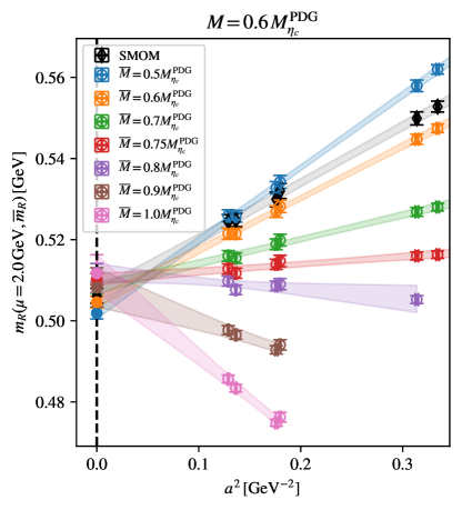
Figure 6: Variations of the renormalization mass scale $\overline{M}$ at fixed value of $M$. The data is fitted to Eq. (18) and the plot displays it after correcting to vanishing residual mass. The black data points show the approach to the continuum for the case of the massless $\mathrm{SMOM}$ scheme. We stress that different values of $\overline{m}$ define different schemes, hence these numbers are not expected to agree in the continuum limit.

We stress that the renormalization mass scale $\overline{m}_{R}$ set by $\overline{M}$ is a scale that can be varied freely within the range where we have data. In Figure 6 we presents fits to the ansatz Eq. (18) $M=0.6\times M_{\eta_{c}}^{\mathrm{PDG}}$ but for a variety of choices of $\overline{M}$. We emphasise again, that the extrapolated values do not have to agree as they are still in different schemes. It is however clearly visible that the approach to the continuum is well described by a fit linear in $a^{2}$ but that the slope varies strongly with the choice of $\overline{M}$. For the largest values of $\overline{M}$ we lose coverage on the coarsest ensembles and hence remove them from the fit. For the remaining analysis we restrict ourselves to values of $\overline{M}$ that allow direct simulations on all considered ensembles.

We also vary the renormalization scale $\mu$ between $2.0\,\mathrm{GeV}$, $2.5\,\mathrm{GeV}$ and $3.0\,\mathrm{GeV}$. We observe that for increasing values of $\mu$ the values of $\overline{M}$ which are required to significantly flatten the continuum limit are beyond the range where we can determine $\overline{m}$ from all three lattice spacings. We therefore base our final results on continuum limit extrapolations at $\mu=2\,\mathrm{GeV}$ and only show the corresponding $\mathrm{mSMOM}$ results obtained from larger scales for comparison (c.f. Table 4).

IV.5 The charm quark mass

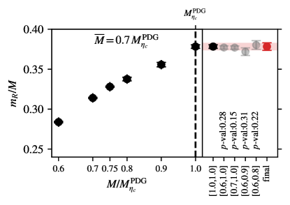
Figure 7: Extrapolation of different intervals of the various reference values $M$ to the physical value $M_{\eta_{c}}^{\mathrm{PDG}}$ at fixed $\overline{M}$. The right hand panel shows results for these interval-choices. The red datapoint to the very right and the corresponding band represents our final value of $m_{c,R}$ in the $\mathrm{mSMOM}$ scheme at $\overline{M}=0.7\,M_{\eta_{c}}^{\mathrm{PDG}}$.

We now vary the choice of $M$ using the various $M_{i}$ and repeat the continuum limit fit for each case, keeping $\overline{M}$ fixed in order to remain in the same scheme. For each choice $M_{i}$ we assemble the error budget of this fit to obtain values $m^{\mathrm{mSMOM}}_{i}(2\,\mathrm{GeV},\overline{m})$. We now combine these results to perform an inter- or extrapolation to the physical charm-quark mass. This is not strictly speaking necessary, since we already have a direct result for this quark mass from the continuum limit at $M_{i}=M_{\eta_{c}}^{\mathrm{PDG}}$, however since this continuum limit is only based on the medium and fine ensembles we prefer to supplement it by a parameterisation using different values (in the continuum) of $m_{i}^{R}/M_{i}$ as a function of $M_{i}$. This is shown in Figure 7. Of our choices for $M_{i}$ we consider the ranges $M_{i}/M_{\eta_{c}}^{\mathrm{PDG}}$ $[0.6,1.0]$, $[0.7,1.0]$, $[0.6,0.9]$ and $[0.6,0.8]$. In each case we parameterise the dependence of the quark mass as a polynomial in $M_{i}$ via

$$\frac{m_{R}}{M}=\alpha M^{-1}+\beta+\gamma M\,.$$ (19)

Table 4: Summary of our final results for the charm quark mass. We quote the renormalization mass scale $\overline{m}_{R}^{\mathrm{mSMOM}}$ defining the given $\mathrm{mSMOM}$ scheme, as well as the charm quark mass in that scheme, converted to $\overline{\mathrm{MS}}$ at the same scale and to $\overline{\mathrm{MS}}$ at $\overline{m}_{c}$. All quark masses are given in units of $\mathrm{GeV}$.

$\mu/\mathrm{GeV}$	$\overline{M}/M_{\eta_{c}}^{\mathrm{PDG}}$	$\overline{m}_{R}(\mu,\overline{m}_{R})$	$m^{\mathrm{RI}}_{c,R}(\mu,\overline{m}_{R})$	$\overline{m}_{c}^{\overline{\mathrm{MS}}}(\mu)$	$\overline{m}_{c}^{\overline{\mathrm{MS}}}(3\,\mathrm{GeV}\leftarrow\mu)$	$\overline{m}_{c}^{\overline{\mathrm{MS}}}(\overline{m}_{c})$
2.0	0.60	0.5046(15)	1.127(7)(12)	1.112(7)(12)(4)	1.005(6)(11)(4)	1.289(6)(10)(3)
2.0	0.70	0.6559(16)	1.129(7)(12)	1.115(7)(12)(4)	1.008(6)(11)(4)	1.292(5)(10)(4)
2.0	0.75	0.7371(16)	1.130(6)(13)	1.118(6)(13)(4)	1.010(6)(11)(4)	1.294(5)(10)(4)
2.0	SMOM	—	1.136(9)(12)	1.114(9)(12)	1.007(8)(10)	1.291(8)(10)
2.5	0.60	0.4698(14)	1.052(7)(14)	1.038(7)(14)(3)	0.995(7)(14)(3)	1.280(6)(13)(3)
2.5	0.70	0.6124(16)	1.057(6)(15)	1.043(6)(15)(3)	1.000(6)(14)(3)	1.284(6)(13)(3)
2.5	0.75	0.6894(16)	1.059(6)(15)	1.046(6)(15)(3)	1.003(6)(15)(3)	1.287(5)(13)(3)
2.5	SMOM	—	1.066(11)(12)	1.048(10)(12)	1.004(10)(12)	1.288(9)(11)
3.0	0.60	0.4450(14)	0.998(7)(15)	0.986(7)(15)(3)	0.986(7)(15)(3)	1.271(6)(14)(2)
3.0	0.70	0.5811(15)	1.004(6)(15)	0.992(6)(15)(3)	0.992(6)(15)(3)	1.277(5)(14)(2)
3.0	0.75	0.6549(16)	1.008(6)(16)	0.995(6)(16)(3)	0.995(6)(16)(3)	1.280(5)(15)(2)
3.0	SMOM	—	1.018(8)(12)	1.002(8)(12)	1.002(8)(12)	1.287(8)(11)

The result to these variations is shown in the right-hand panel of Figure 7. We take the direct determination at the charm quark mass (i.e. $M_{i}=M_{\eta_{c}}^{\mathrm{PDG}}$) as central value and in addition to its uncertainty we conservatively associate a systematic uncertainty of half the spread of the variation. These fit results that determine this uncertainty are shown in the right hand panel of Figure 7. We quote the two uncertainties separately, since the latter only arises since we require our final number to be based on continuum limits from more than two lattice spacings. With additional finer ensembles, this last uncertainty would be completely removed, since a continuum limit with three lattice spacings could be obtained directly at the charm quark mass. We then repeat the analysis for different choices of $\overline{M}$ (and hence $\overline{m}_{R}$) as well as the massless $\mathrm{SMOM}$ scheme.

Finally, it remains to convert these results into a common scheme where they can be directly compared to each other. Using the conversion factor $R_{m}^{\overline{\mathrm{MS}}\leftarrow\mathrm{mSMOM}}$ given in Eq. (41), we can convert the results from $m_{c,R}^{\mathrm{mSMOM}}(\mu,\overline{m}_{R})$ to $m_{c,R}^{\overline{\mathrm{MS}}}(\mu)$. Unfortunately, for the $\mathrm{mSMOM}$ scheme, this is currently only known at one loop. In order to quantify the truncation effects in the temporary absence of perturbative two-loop calculations, we investigate the difference between one- and two-loop corrections for the massless scheme Gorbahn and Jager (2010); Almeida and Sturm (2010) and assign the relative difference between them as a systematic truncation uncertainty. In practice we find that for $\mu=2.0\,\mathrm{GeV}$ ($2.5\,\mathrm{GeV}$, $3.0\,\mathrm{GeV}$) the difference between 1- and 2-loop conversion to $\overline{\mathrm{MS}}$ is a 0.38% (0.31%, 0.27%) effect. Within the $\overline{\mathrm{MS}}$ scheme we then run the results up to $3\,\mathrm{GeV}$ as well as down to the charm quark scale to quote $\overline{m}_{c}(\overline{m}_{c})$. To compute the strong coupling and running of the ${\overline{\text{MS}}}$ quark mass we make use of RunDec Chetyrkin et al. (2000); Schmidt and Steinhauser (2012); Herren and Steinhauser (2018), which in turn relies on 5-loop results for the beta function and for the mass anomalous dimension Baikov et al. (2014); Luthe et al. (2017a); Baikov et al. (2017a, b); Herzog et al. (2017); Luthe et al. (2017b).

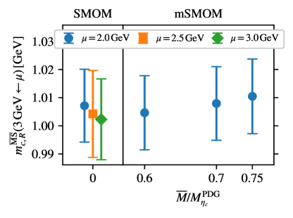
Figure 8: Results for the continuum-extrapolated renormalized charm quark mass converted to $\overline{\mathrm{MS}}$ from RI/SMOM and RI/mSMOM with variation in $\overline{M}$ at renormalization scale of 3 GeV using results from $\mu=2.0,2.5,3.0\,\mathrm{GeV}$. Numerical values are presented in Table 4.

We list these results for some choices of $\overline{M}$ and $\mu$ in Table 4 where the first uncertainty is the result from the pure $\mathrm{mSMOM}$ calculation at at a chosen quark mass, the second uncertainty lists encapsulates the charm-mass interpolation, and the last uncertainty estimates the truncation effect due to performing the matching at 1-loop. In principle one could also quote a fourth uncertainty encapsulating the uncertainties of the inputs to the running and the truncation of the running factor, however these are found to be negligible.

Our final results for the charm quark mass converted to $\overline{\mathrm{MS}}$ and then (where necessary) ran to $3\,\mathrm{GeV}$ within the $\overline{\mathrm{MS}}$ scheme are shown in Figure 8. As mentioned above, in the massive scheme the continuum limit is well controlled for determinations at $\mu=2$ but values of $\overline{M}$ which significantly decrease the slope of the continuum limit are not reachable on our current data set for larger values of $\mu$ and we therefore exclude them. We find good agreement between the $\mathrm{SMOM}$ and the $\mathrm{mSMOM}$ schemes as well as amongst different values for $\overline{m}_{R}$ within the $\mathrm{mSMOM}$ scheme. As our final number we quote our results obtained from $\mathrm{mSMOM}$ at $\hat{\mu}=2\,\mathrm{GeV}$ from the choice $\overline{M}=0.7\,M_{\eta_{c}}^{\mathrm{PDG}}$ which corresponds to $\overline{m}_{R}^{\mathrm{mSMOM}}=0.6559(16)\,\mathrm{GeV}$. We find

$$m^{\mathrm{mSMOM}}_{c,R}(2\,\mathrm{GeV},\overline{m}_{R}) =1.129(7)(12)\,\mathrm{GeV}\,,$$ (20)

$$m^{\overline{\mathrm{MS}}}_{c,R}(2\,\mathrm{GeV}) =1.115(7)(12)(4)\,\mathrm{GeV}\,,$$ (21)

$$m^{\overline{\mathrm{MS}}}_{c,R}(3\,\mathrm{GeV}) =1.008(6)(11)(4)\,\mathrm{GeV}\,,$$ (22)

$$m^{\overline{\mathrm{MS}}}_{c,R}(m^{\overline{\mathrm{MS}}}_{c,R}) =1.292(5)(10)(4)\,\mathrm{GeV}\,.$$ (23)

The first uncertainty comes from the determination directly at the charm quark mass, the second from the inter-/extrapolation taking smaller than physical reference values, the third from the perturbative truncation uncertainty when converting to $\overline{\mathrm{MS}}$. We have not applied any additional uncertainties associated with the running within $\overline{\mathrm{MS}}$.

IV.6 Comparison to the literature

The charm quark mass has been previously computed by various collaborations in various schemes. In Figure 9 we compare our result to the results in the literature which enter the FLAG average in the $\overline{\mathrm{MS}}$ scheme at $3\,\mathrm{GeV}$ We find good agreement with other $N_{f}=2+1$ calculations and obtain similar uncertainties. The leading uncertainty in our calculation arises from the fact that not all the ensembles we currently use allow for direct simulation at the physical charm quark mass. Using an additional finer lattice spacing will allow to eliminate this uncertainty in the future.

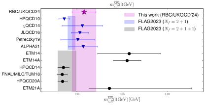
Figure 9: Comparison of our result with previous determinations of the charm quark mass in the literature that enter the FLAG Aoki et al. (2022) average. The magenta star and corresponding band are our result, the blue triangles are results based on $N_{f}=2+1$ Heitger et al. (2021); Petreczky and Weber (2019); Nakayama et al. (2016); Yang et al. (2015); McNeile et al. (2010) and the black circles based on $N_{f}=2+1+1$ Alexandrou et al. (2021); Hatton et al. (2020); Bazavov et al. (2018); Alexandrou et al. (2014); Chakraborty et al. (2015); Carrasco et al. (2014). The blue and black bands show the corresponding FLAG averages for $N_{f}=2+1$ and $N_{f}=2+1+1$, respectively.

V Summary and Outlook

We have presented the first numerical implementation of the massive non-perturbative renormalization scheme which was first suggested in Ref. Boyle et al. (2017a). We find that varying the mass scale at which the renormalization conditions are imposed can be used to significantly modify the approach to the continuum limit, and in particular to flatten it. We observe good agreement between different renormalization mass scales (and hence continuum limit approaches), further substantiating that the continuum limit is controlled.

This scheme can be applied to any observable and hence be used to obtain more reliable continuum limits. Since different choices of the renormalization mass scale must agree in the continuum limit, it also provides non-trivial tests allowing to scrutinise a given continuum limit by performing it for different choices of the renormalization scheme mass scale. This is not restricted to heavy-quark observables but is useful for any observable with large discretisation effects compared to the desired statistical precision.

The joint continuum limit fits to the chosen Möbius und Shamir domain wall kernels with very similar lattice spacings agree well with only fitting the Möbius ensembles and (at the present level of precision) are well described by an ansatz that is linear in $a^{2}$. We obtain the charm quark mass in the $\overline{\mathrm{MS}}$ scheme at $3\,\mathrm{GeV}$ with a precision of 1.3% in good agreement with the literature. This uncertainty can be significantly reduced by using additional finer ensembles. By direct computation, we find the sea-pion effect on the charmed meson mass $M_{\eta_{c}}$ between a pion mass of $286\,\mathrm{MeV}$ and the physical pion mass to be below the permille level.

For the future, we envisage applications of the $\mathrm{mSMOM}$ scheme to other observables and an extension to four quark operators.

Appendix A Numerical results

In tables 5- 10 we summarise the numerical data for the residual mass, $Z_{A}$, the hadron mass $aM$ as well as the renormalization constant $Z_{m}$ interpolated to a scale of $2\,\mathrm{GeV}$.

Table 5: Summary of numerical results on the C1M ensemble used for the analysis. The values of $Z_{m}$ are given after interpolation to $\mu=2\,\mathrm{GeV}$.

C1M	$10^{3}am_{\mathrm{res}}$	$aM$	$Z_{A}$	$Z^{\mathrm{mSMOM}}_{m}$	$Z_{m}^{\mathrm{SMOM}}$
0.0050	0.601(12)	0.1642(34)	0.71302(34)	1.5754(65)	1.5428(15)
0.0100	0.574(11)	0.2203(22)	0.71337(19)	1.6088(36)	1.5442(12)
0.0181	0.5330(95)	0.2886(14)	0.71443(12)	1.6211(22)	1.5425(11)
0.0362	0.4642(79)	0.40331(87)	0.717257(77)	1.6232(15)	1.5362(10)
0.0500	0.450(17)	0.4769(22)	0.71979(19)	1.6185(14)	-
0.1000	0.361(12)	0.6877(14)	0.72921(11)	1.5996(12)	-
0.1500	0.3210(100)	0.8637(11)	0.74087(11)	1.5725(10)	-
0.2000	0.3172(94)	1.01971(85)	0.75528(13)	1.53813(93)	-
0.3000	0.599(16)	1.28930(50)	0.79647(16)	1.44377(74)	-

Table 6: Summary of numerical results on the C1S ensemble used for the analysis. The values of $Z_{m}$ are given after interpolation to $\mu=2\,\mathrm{GeV}$.

C1S	$10^{3}am_{\mathrm{res}}$	$aM$	$Z_{A}$	$Z^{\mathrm{mSMOM}}_{m}$	$Z_{m}^{\mathrm{SMOM}}$
0.0050	3.162(19)	0.1885(29)	0.71796(44)	1.3145(75)	1.5410(19)
0.0100	3.085(18)	0.2367(21)	0.71822(28)	1.4381(35)	1.5411(14)
0.0200	2.938(16)	0.3129(15)	0.71942(17)	1.5245(18)	1.5392(12)
0.0400	2.720(12)	0.4304(10)	0.72235(12)	1.5706(12)	1.5325(12)
0.0500	2.644(22)	0.4829(18)	0.72413(27)	1.5772(14)	-
0.1000	2.427(15)	0.6904(14)	0.73344(23)	1.5763(12)	-
0.1500	2.420(11)	0.8636(11)	0.74507(19)	1.5542(11)	-
0.2000	2.6192(92)	1.01733(94)	0.75960(15)	1.5210(10)	-
0.3000	4.530(18)	1.28409(79)	0.80194(14)	1.42069(78)	-
0.3300	6.455(18)	1.35527(38)	0.821474(90)	1.37464(67)	-

Table 7: Summary of numerical results on the M1M ensemble used for the analysis. The values of $Z_{m}$ are given after interpolation to $\mu=2\,\mathrm{GeV}$.

M1M	$10^{3}am_{\mathrm{res}}$	$aM$	$Z_{A}$	$Z^{\mathrm{mSMOM}}_{m}$	$Z_{m}^{\mathrm{SMOM}}$
0.0040	0.3116(61)	0.1196(26)	0.74376(24)	1.5167(51)	1.5743(21)
0.0080	0.3018(56)	0.1651(16)	0.74421(13)	1.5635(26)	1.5722(23)
0.0133	0.2907(51)	0.2113(12)	0.744798(86)	1.5820(20)	1.5709(20)
0.0266	0.2709(39)	0.29939(79)	0.746330(56)	1.5955(18)	1.5667(18)
0.0500	0.2527(54)	0.4178(17)	0.749495(88)	1.5970(16)	-
0.1000	0.2414(40)	0.6163(11)	0.757548(60)	1.5851(15)	-
0.1500	0.2523(35)	0.78311(79)	0.767843(47)	1.5612(14)	-
0.2250	0.3173(27)	1.00082(63)	0.788084(41)	1.5093(11)	-
0.3000	0.5277(20)	1.19017(57)	0.815321(43)	1.44227(90)	-
0.3200	0.6634(21)	1.23610(64)	0.824062(46)	1.42193(84)	-
0.3400	0.8998(26)	1.28063(63)	0.833810(56)	1.39986(79)	-

Table 8: Summary of numerical results on the M1S ensemble used for the analysis. The values of $Z_{m}$ are given after interpolation to $\mu=2\,\mathrm{GeV}$.

M1S	$10^{3}am_{\mathrm{res}}$	$aM$	$Z_{A}$	$Z^{\mathrm{mSMOM}}_{m}$	$Z_{m}^{\mathrm{SMOM}}$
0.0040	0.6727(72)	0.1290(24)	0.74486(27)	1.5055(58)	1.5720(26)
0.0080	0.6561(64)	0.1714(16)	0.74542(15)	1.5557(28)	1.5708(21)
0.0150	0.6319(55)	0.2283(11)	0.746212(91)	1.5802(19)	1.5690(19)
0.0300	0.5977(42)	0.32118(69)	0.747987(58)	1.5930(18)	1.5639(18)
0.0500	0.5767(52)	0.42023(76)	0.75062(11)	1.5951(18)	-
0.1000	0.5479(35)	0.61780(44)	0.758721(100)	1.5838(17)	-
0.1500	0.5602(29)	0.78382(43)	0.769158(89)	1.5596(15)	-
0.2250	0.6677(29)	1.00056(52)	0.789767(76)	1.5066(13)	-
0.3000	1.0409(41)	1.18880(56)	0.817587(74)	1.43775(99)	-
0.3200	1.2562(65)	1.23385(41)	0.826456(79)	1.41695(97)	-
0.3400	1.6053(82)	1.27801(40)	0.836317(81)	1.39437(87)	-
0.3600	2.189(11)	1.32043(39)	0.847392(85)	1.36951(81)	-
0.3750	2.936(12)	1.35187(55)	0.857047(90)	1.34809(77)	-

Table 9: Summary of numerical results on the F1M ensemble used for the analysis. The values of $Z_{m}$ are given after interpolation to $\mu=2\,\mathrm{GeV}$.

F1M	$10^{3}am_{\mathrm{res}}$	$aM$	$Z_{A}$	$Z^{\mathrm{mSMOM}}_{m}$	$Z_{m}^{\mathrm{SMOM}}$
0.0021	0.2399(56)	0.0865(21)	0.75927(21)	1.4816(57)	1.5797(23)
0.0043	0.2390(52)	0.1172(16)	0.75952(11)	1.5229(31)	1.5802(21)
0.0107	0.2343(43)	0.1795(10)	0.760226(53)	1.5766(21)	1.5792(19)
0.0214	0.2286(36)	0.25287(54)	0.761281(42)	1.5924(20)	1.5759(18)
0.0330	0.2244(31)	0.31620(38)	0.762536(41)	1.5942(19)	-
0.0660	0.2201(21)	0.46183(32)	0.766829(40)	1.5935(19)	-
0.0990	0.2248(15)	0.58391(32)	0.772132(39)	1.5838(18)	-
0.1320	0.2378(12)	0.69368(30)	0.778456(38)	1.5683(16)	-
0.1980	0.29064(77)	0.88979(25)	0.794371(35)	1.5243(14)	-
0.2640	0.39970(57)	1.06271(21)	0.815121(32)	1.4682(11)	-
0.3300	0.66808(62)	1.21606(19)	0.841614(31)	1.40308(87)	-
0.3600	1.0280(12)	1.27967(19)	0.856367(32)	1.36962(80)	-

Table 10: Summary of numerical results on the F1S ensemble used for the analysis. The values of $Z_{m}$ are given after interpolation to $\mu=2\,\mathrm{GeV}$.

F1S	$10^{3}am_{\mathrm{res}}$	$aM$	$Z_{A}$	$Z^{\mathrm{mSMOM}}_{m}$	$Z_{m}^{\mathrm{SMOM}}$
0.0021	0.9769(95)	0.0994(18)	0.76231(18)	1.4979(67)	1.5802(18)
0.0043	0.9722(88)	0.1263(13)	0.76263(11)	1.5265(38)	1.5809(18)
0.0107	0.9565(62)	0.18387(86)	0.763139(55)	1.5759(23)	1.5802(17)
0.0214	0.9393(43)	0.25453(57)	0.764180(44)	1.5918(19)	1.5768(17)
0.0330	0.9291(36)	0.31626(41)	0.765486(42)	1.5935(20)	-
0.0660	0.9188(24)	0.45975(34)	0.769873(38)	1.5923(19)	-
0.0990	0.9251(18)	0.58074(34)	0.775231(37)	1.5822(17)	-
0.1320	0.9463(14)	0.68965(34)	0.781619(36)	1.5662(16)	-
0.1980	1.0427(11)	0.88429(32)	0.797730(37)	1.5208(13)	-
0.2640	1.2577(11)	1.05584(28)	0.818823(38)	1.4630(10)	-
0.3300	1.7485(18)	1.20763(25)	0.845736(38)	1.39618(82)	-
0.3960	3.1873(46)	1.34062(22)	0.880386(40)	1.31942(65)	-

Appendix B Mass conversion factor

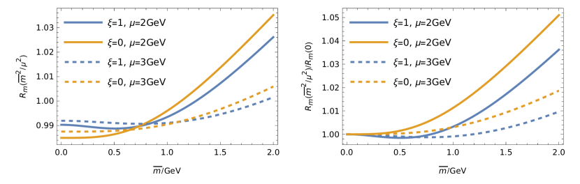
Figure 10: Left: conversion factor $R_{m}^{{\overline{\text{MS}}}\leftarrow\text{mSMOM}}(m^{2}/\mu^{2})$ for $0<m<2\,\text{GeV}$. Right, ratio $R_{m}^{{\overline{\text{MS}}}\leftarrow\text{mSMOM}}(m^{2}/\mu^{2})/R_{m}^{{\overline{\text{MS}}}\leftarrow\text{mSMOM}}(0)=R_{m}^{\text{SMOM}\leftarrow\text{mSMOM}}(m^{2}/\mu^{2})$. Both plots show curves with $(\alpha,\mu)=(0.293347,2\,\text{GeV})$ (solid) and $(\alpha,\mu)=(0.24358,3\,\text{GeV})$ (dashed), and for gauge-parameter $\xi$ set to $1$ (Feynman gauge) or $0$ (Landau gauge). The dimensional regularisation scale $\tilde{\mu}$ is set to $\mu$.

Here we determine the mSMOM to ${\overline{\text{MS}}}$ conversion factor for the mass at one-loop in continuum perturbation theory, with an arbitrary choice of the gauge parameter $\xi$. We work in Minkowski space, with fermion propagator

$$S(p)=\frac{i}{\not{p}-m-\Sigma(p)+i\epsilon}\,.$$ (24)

We use dimensional regularisation in $d=4-2\epsilon$ dimensions, denoting by $\tilde{\mu}$ the dimensionful scale introduced (to distinguish it from the scale $\mu$ defining the mSMOM symmetric-momentum point). We compute the fermion self-energy to find the wave-function renormalization and then determine $Z^{\text{mSMOM}}_{m}$ by using the mSMOM renormalization from equation (4), which in Minkowski space reads

$$1 =\frac{1}{12m_{R}}\Big{\{}\mathop{\text{Tr}}[-iS_{R}(p)^{-1}]_{p^{2}=-\mu^{2}}$$ (25)

$$\phantom{=\frac{1}{12m_{R}}}{}\;\;\;-\frac{1}{2}\mathop{\text{Tr}}[q{\cdot}\Lambda_{\text{A},R}\gamma_{5}]_{\text{sym}}\Big{\}}.$$

The conversion factor is given by

$$R_{m}^{{\overline{\text{MS}}}\leftarrow\text{mSMOM}}=Z_{m}^{\overline{\text{MS}}}/Z^{\text{mSMOM}}_{m}.$$ (26)

The one-loop self-energy integral is

$$-i\Sigma^{(1)}(p)=-g^{2}\tilde{\mu}^{2\epsilon}C_{F}\int\frac{d^{d}k}{(2\pi)^{d}}\left[\frac{\gamma_{\mu}(\not{p}-\not{k}+m)\gamma^{\mu}}{k^{2}\big{(}(p-k)^{2}-m^{2}\big{)}}-(1-\xi)\frac{\not{k}(\not{p}-\not{k}+m)\not{k}}{(k^{2})^{2}\big{(}(p-k)^{2}-m^{2}\big{)}}\right],$$ (27)

where $C_{F}=4/3$ is the $\text{SU}(3)$ quadratic Casimir operator in the fundamental representation. This can be evaluated by standard techniques, using Mathematica Mat (2024) to perform the Feynman-parameter integrals. The result is

$$\Sigma^{(1)}(p) =\frac{\alpha}{4\pi}C_{F}\!\!\left[\not{p}\,\xi\left(-\frac{1}{\overline{\epsilon}}-1+u+u^{2}\ln\Big{(}\!\frac{u}{1+u}\!\Big{)}+\ln(1+u)+\ln(\mu^{2}/\tilde{\mu}^{2})\right)\right.$$ (28)

$$\phantom{=\frac{\alpha}{4\pi}C_{F}}\left.{}+m\left(4+2\xi+(3+\xi)\Big{(}\frac{1}{\overline{\epsilon}}+u\ln\Big{(}\!\frac{u}{1+u}\!\Big{)}-\ln(1+u)-\ln(\mu^{2}/\tilde{\mu}^{2}\Big{)}\right)\right]$$

$$=\frac{\alpha}{4\pi}C_{F}\,[\not{p}A_{\xi}+mB_{\xi}],$$

where we have set $u=m^{2}/\mu^{2}$ and have defined

$$\frac{1}{\overline{\epsilon}}\equiv\frac{1}{\epsilon}-\gamma_{\text{E}}+\ln(4\pi).$$ (29)

When $\xi=1$ the result for $\Sigma^{(1)}(p)$ above agrees with equation (37) in Ref. Boyle et al. (2017a). From this, the mSMOM wave-function renormalization constant, up to one loop, is

$$Z^{\text{mSMOM}}_{q}=1-\frac{\alpha}{4\pi}C_{F}\,A_{\xi}.$$ (30)

Now write the one-loop contribution to an amputated bilinear vertex as $\Lambda^{(1)}_{\Gamma}=\Lambda^{(1)}_{\Gamma,\xi=1}+\Lambda^{(1)}_{\Gamma,\xi\neq 1}$, with:

$$\Lambda^{(1)}_{\Gamma,\xi=1} =-ig^{2}\tilde{\mu}^{2\epsilon}C_{F}\int\frac{d^{d}k}{(2\pi)^{d}}\,\frac{\gamma_{\mu}(\not{p}_{3}-\not{k}+m)\Gamma(\not{p}_{2}-\not{k}+m)\gamma^{\mu}}{k^{2}\big{(}(p_{3}-k)^{2}-m^{2}\big{)}\big{(}(p_{2}-k)^{2}-m^{2}\big{)}},$$ (31)

$$\Lambda^{(1)}_{\Gamma,\xi\neq 1} =ig^{2}\tilde{\mu}^{2\epsilon}C_{F}\,(1-\xi)\int\frac{d^{d}k}{(2\pi)^{d}}\,\frac{\not{k}(\not{p}_{3}-\not{k}+m)\Gamma(\not{p}_{2}-\not{k}+m)\not{k}/k^{2}}{k^{2}\big{(}(p_{3}-k)^{2}-m^{2}\big{)}\big{(}(p_{2}-k)^{2}-m^{2}\big{)}}.$$ (32)

The renormalization condition above requires us to compute $\mathop{\text{Tr}}[q\cdot\Lambda^{(1)}_{\text{A}}\gamma_{5}]$, with $\Gamma^{\nu}_{\text{A}}=\gamma^{\nu}\gamma_{5}$. By tracing the numerators of the two integrands for $\xi=1$ and $\xi\neq 1$, we see that

$$\mathop{\text{Tr}}[\Lambda^{(1)}_{\text{A,$\xi\neq 1$}}\gamma_{5}]=-\frac{1-\xi}{d}\mathop{\text{Tr}}[\Lambda^{(1)}_{\text{A,$\xi=1$}}\gamma_{5}].$$ (33)

Hence we have to evaluate only the $\xi=1$ (Feynman gauge) term for $\mathop{\text{Tr}}[\Lambda^{(1)}_{\text{A,$\xi=1$}}\gamma_{5}]$. Using the notation,

$$N_{\Gamma}=\gamma_{\mu}(\not{p}_{3}-\not{k}+m)\,\Gamma\,(\not{p}_{2}-\not{k}+m)\gamma^{\mu},$$ (34)

we have

$$\mathop{\text{Tr}}[q\cdot N_{\text{A}}\gamma_{5}]=12mdq^{2}$$ (35)

and we learn that $\mathop{\text{Tr}}[q\cdot\Lambda^{(1)}_{\text{A,$\xi=1$}}\gamma_{5}]$ can be expressed in terms of the finite integral

$$-ig^{2}\tilde{\mu}^{2\epsilon}C_{F}\!\!\int\!\!\frac{d^{d}k}{(2\pi)^{d}}\,\frac{1}{k^{2}\big{(}(p_{3}{-}k)^{2}-m^{2}\big{)}\big{(}(p_{2}{-}k)^{2}-m^{2}\big{)}}\\ =-\frac{\alpha}{4\pi}C_{F}\frac{1}{\mu^{2}}C_{0}(m^{2}/\mu^{2}),$$ (36)

where $C_{0}(u)$ comes from a Feynman-parameter integral and is given by

$$C_{0}(u)=\frac{2i}{\sqrt{3}}\left[\text{Li}_{2}\Big{(}\frac{-i+\sqrt{3}}{\sqrt{3}-i\sqrt{4u+1}}\Big{)}\right.-\left.\text{Li}_{2}\Big{(}\frac{i+\sqrt{3}}{\sqrt{3}-i\sqrt{4u+1}}\Big{)}\right.+\left.\text{Li}_{2}\Big{(}\frac{-i+\sqrt{3}}{i\sqrt{4u+1}+\sqrt{3}}\Big{)}\right.-\left.\text{Li}_{2}\Big{(}\frac{i+\sqrt{3}}{i\sqrt{4u+1}+\sqrt{3}}\Big{)}\right].$$ (37)

Since the result is finite, we can set $d=4$ and find

$$\mathop{\text{Tr}}[q{\cdot}\Lambda^{(1)}_{\text{A}}\gamma_{5}]_{\text{sym}}=\Big{(}1-\frac{1-\xi}{4}\Big{)}\mathop{\text{Tr}}[q{\cdot}\Lambda^{(1)}_{\text{A},\xi=1}\gamma_{5}]_{\text{sym}}=12m\frac{\alpha}{4\pi}C_{F}(3+\xi)C_{0}(m^{2}/\mu^{2}).$$ (38)

Now we have all we need to evaluate $Z^{\text{mSMOM}}_{m}$ from the renormalization condition in (25), which we rewrite as

$$Z_{m}^{\text{mSMOM}}=\lim_{m_{\text{R}}\to{\overline{m}}}\frac{1}{12m}\frac{1}{Z_{q}^{\text{mSMOM}}}\left[\mathop{\text{Tr}}\big{(}{-i}S(p)^{-1}\big{)}_{p^{2}=-\mu^{2}}-\frac{1}{2}Z_{\text{A}}^{\text{mSMOM}}\mathop{\text{Tr}}(q\cdot\Lambda_{\text{A}}\gamma_{5})_{\text{sym}}\right].$$ (39)

Using the results in (28), (30) and (38), together with (in Minkowski space) $iS(p)^{-1}=\not{p}-m-\Sigma(p)$, shows that to one loop,

$$Z^{\text{mSMOM}}_{m} =1+\frac{\alpha}{4\pi}C_{F}\left[A_{\xi}+B_{\xi}-\frac{3+\xi}{2}C_{0}({\overline{m}}^{2}/\mu^{2})\right]$$ (40)

$$=1+\frac{\alpha}{4\pi}C_{F}\left[3\frac{1}{\overline{\epsilon}}+(4+\xi)-\frac{3+\xi}{2}\,C_{0}(u)-3\ln(\mu^{2}/\tilde{\mu}^{2})\right.$$

$$\phantom{=1+\frac{\alpha}{4\pi}C_{F}}\left.{}\;+\xi\bigg{(}u+u^{2}\ln\Big{(}\frac{u}{1+u}\Big{)}\bigg{)}+(3+\xi)\,u\ln\Big{(}\frac{u}{1+u}\Big{)}-3\ln(1+u)\right],$$

where now $u={\overline{m}}^{2}/\mu^{2}$. Finally, the conversion factor is:

$$R_{m}^{{\overline{\text{MS}}}\leftarrow\text{mSMOM}} =1+\frac{\alpha}{4\pi}C_{F}\left[-(4+\xi)+\frac{3+\xi}{2}\,C_{0}(u)+3\ln(\mu^{2}/\tilde{\mu}^{2})+3\ln(1+u)\right.$$ (41)

$$\phantom{=1+\frac{\alpha}{4\pi}C_{F}}\left.{}\;-\xi\bigg{(}u+u^{2}\ln\Big{(}\frac{u}{1+u}\Big{)}\bigg{)}-(3+\xi)\,u\ln\Big{(}\frac{u}{1+u}\Big{)}\right].$$

When $\bar{m}\to 0$ ($u\to 0$), this agrees with equation (24) in Sturm et al Sturm et al. (2009), after setting $\tilde{\mu}=\mu$. For $\xi=1$ the result for $Z^{\text{mSMOM}}_{\text{P}}=1/Z^{\text{mSMOM}}_{m}$ reproduces the Feynman-gauge result in Ref. Boyle et al. (2017a). We also computed $Z^{\text{mSMOM}}_{\text{P}}$ to one-loop order directly from the renormalization condition of equation (7) (in Minkowski space) and confirmed that $Z^{\text{mSMOM}}_{\text{P}}=1/Z^{\text{mSMOM}}_{m}$ for arbitrary $\xi$.

The lattice computations are performed using Landau-gauge-fixed configurations and hence we need the conversion factor in Landau gauge, $\xi=0$:

$$R_{m}^{{\overline{\text{MS}}}\leftarrow\text{mSMOM}}=1+\frac{\alpha}{4\pi}C_{F}\left[-4+\frac{3}{2}\,C_{0}(u)+3\ln(\mu^{2}/\tilde{\mu}^{2})+3\ln(1+u)-3u\ln\Big{(}\frac{u}{1+u}\Big{)}\right].$$ (42)

In figure 10, we show plots of the mass conversion factor as a function of ${\overline{m}}$, in both Feynman and Landau gauge for two choices of matching scale $\mu$ (taking $\tilde{\mu}=\mu$).

References

- Boyle et al. (2017a) Peter Boyle, Luigi Del Debbio, and Ava Khamseh, “Massive momentum-subtraction scheme,” Phys. Rev. D 95, 054505 (2017a), arXiv:1611.06908 [hep-lat] .
- Del Debbio et al. (2023) Luigi Del Debbio, Felix Erben, Jonathan Flynn, Rajnandini Mukherjee, and J. Tobias Tsang, “Charm quark mass using a massive nonperturbative renormalisation scheme,” (2023), arXiv:2312.16537 [hep-lat] .
- Aoki et al. (2011) Y. Aoki et al., “Continuum Limit of from 2+1 Flavor Domain Wall QCD,” Phys. Rev. D 84, 014503 (2011), arXiv:1012.4178 [hep-lat] .
- Blum et al. (2016) T. Blum et al. (RBC, UKQCD), “Domain wall QCD with physical quark masses,” Phys. Rev. D 93, 074505 (2016), arXiv:1411.7017 [hep-lat] .
- Boyle et al. (2017b) Peter A. Boyle, Luigi Del Debbio, Andreas Jüttner, Ava Khamseh, Francesco Sanfilippo, and Justus Tobias Tsang, “The decay constants and in the continuum limit of domain wall lattice QCD,” JHEP 12, 008 (2017b), arXiv:1701.02644 [hep-lat] .
- Boyle et al. (2018) Peter A. Boyle, Luigi Del Debbio, Nicolas Garron, Andreas Juttner, Amarjit Soni, Justus Tobias Tsang, and Oliver Witzel (RBC/UKQCD), “SU(3)-breaking ratios for and mesons,” (2018), arXiv:1812.08791 [hep-lat] .
- Boyle et al. (2024) Peter A. Boyle, Felix Erben, Jonathan M. Flynn, Nicolas Garron, Julia Kettle, Rajnandini Mukherjee, and J. Tobias Tsang, “Kaon mixing beyond the standard model with physical masses,” (2024), arXiv:2404.02297 [hep-lat] .
- Iwasaki and Yoshie (1984) Y. Iwasaki and T. Yoshie, “Renormalization Group Improved Action for SU(3) Lattice Gauge Theory and the String Tension,” Phys. Lett. 143B, 449–452 (1984).
- Iwasaki (1985) Y. Iwasaki, “Renormalization Group Analysis of Lattice Theories and Improved Lattice Action: Two-Dimensional Nonlinear O(N) Sigma Model,” Nucl. Phys. B258, 141–156 (1985).
- Shamir (1993) Yigal Shamir, “Chiral fermions from lattice boundaries,” Nucl.Phys. B406, 90–106 (1993), arXiv:hep-lat/9303005 [hep-lat] .
- Furman and Shamir (1995) Vadim Furman and Yigal Shamir, “Axial symmetries in lattice QCD with Kaplan fermions,” Nucl.Phys. B439, 54–78 (1995), arXiv:hep-lat/9405004 [hep-lat] .
- Brower et al. (2005) Richard C. Brower, Hartmut Neff, and Kostas Orginos, “Mobius fermions: Improved domain wall chiral fermions,” Nucl.Phys.Proc.Suppl. 140, 686–688 (2005), arXiv:hep-lat/0409118 [hep-lat] .
- Brower et al. (2006) R.C. Brower, H. Neff, and K. Orginos, “Mobius fermions,” Nucl.Phys.Proc.Suppl. 153, 191–198 (2006), arXiv:hep-lat/0511031 [hep-lat] .
- Brower et al. (2017) Richard C. Brower, Harmut Neff, and Kostas Orginos, “The Möbius domain wall fermion algorithm,” Comput. Phys. Commun. 220, 1–19 (2017), arXiv:1206.5214 [hep-lat] .
- Boyle et al. (2016a) Peter Boyle, Andreas Juttner, Marina Krstic Marinkovic, Francesco Sanfilippo, Matthew Spraggs, and Justus Tobias Tsang, “An exploratory study of heavy domain wall fermions on the lattice,” JHEP 04, 037 (2016a), arXiv:1602.04118 [hep-lat] .
- Boyle et al. (2016b) Peter A. Boyle, Guido Cossu, Azusa Yamaguchi, and Antonin Portelli, “Grid: A next generation data parallel C++ QCD library,” PoS LATTICE2015, 023 (2016b).
- Yamaguchi et al. (2022) Azusa Yamaguchi, Peter Boyle, Guido Cossu, Gianluca Filaci, Christoph Lehner, and Antonin Portelli, “Grid: OneCode and FourAPIs,” PoS LATTICE2021, 035 (2022), arXiv:2203.06777 [hep-lat] .
- Portelli et al. (2023) Antonin Portelli, Nelson Lachini, Felix Erben, Michael Marshall, Fabian Joswig, Raoul Hodgson, Fionn Ó hÓgáin, Vera Gülpers, Peter Boyle, Nils Asmussen, Ryan Hill, Alessandro Barone, James Richings, Ryan Abbott, Simon Bürger, and Joseph Lee, “aportelli/hadrons: Hadrons v1.4,” (2023).
- Blum et al. (2004) T. Blum, P. Chen, Norman H. Christ, C. Cristian, C. Dawson, et al., “Quenched lattice QCD with domain wall fermions and the chiral limit,” Phys.Rev. D69, 074502 (2004), arXiv:hep-lat/0007038 [hep-lat] .
- Boyle (2014) P. A. Boyle, “Conserved currents for Mobius Domain Wall Fermions,” (2014), arXiv:1411.5728 [hep-lat] .
- Davies et al. (2010) C. T. H. Davies, C. McNeile, E. Follana, G. P. Lepage, H. Na, and J. Shigemitsu, “Update: Precision decay constant from full lattice QCD using very fine lattices,” Phys. Rev. D 82, 114504 (2010), arXiv:1008.4018 [hep-lat] .
- Workman et al. (2022) R. L. Workman et al. (Particle Data Group), “Review of Particle Physics,” PTEP 2022, 083C01 (2022).
- Gorbahn and Jager (2010) Martin Gorbahn and Sebastian Jager, “Precise MS-bar light-quark masses from lattice QCD in the RI/SMOM scheme,” Phys. Rev. D 82, 114001 (2010), arXiv:1004.3997 [hep-ph] .
- Almeida and Sturm (2010) Leandro G. Almeida and Christian Sturm, “Two-loop matching factors for light quark masses and three-loop mass anomalous dimensions in the RI/SMOM schemes,” Phys. Rev. D 82, 054017 (2010), arXiv:1004.4613 [hep-ph] .
- Chetyrkin et al. (2000) K. G. Chetyrkin, Johann H. Kuhn, and M. Steinhauser, “RunDec: A Mathematica package for running and decoupling of the strong coupling and quark masses,” Comput. Phys. Commun. 133, 43–65 (2000), arXiv:hep-ph/0004189 .
- Schmidt and Steinhauser (2012) Barbara Schmidt and Matthias Steinhauser, “CRunDec: a C++ package for running and decoupling of the strong coupling and quark masses,” Comput. Phys. Commun. 183, 1845–1848 (2012), arXiv:1201.6149 [hep-ph] .
- Herren and Steinhauser (2018) Florian Herren and Matthias Steinhauser, “Version 3 of RunDec and CRunDec,” Comput. Phys. Commun. 224, 333–345 (2018), arXiv:1703.03751 [hep-ph] .
- Baikov et al. (2014) P. A. Baikov, K. G. Chetyrkin, and J. H. Kühn, “Quark Mass and Field Anomalous Dimensions to ,” JHEP 10, 076 (2014), arXiv:1402.6611 [hep-ph] .
- Luthe et al. (2017a) Thomas Luthe, Andreas Maier, Peter Marquard, and York Schröder, “Five-loop quark mass and field anomalous dimensions for a general gauge group,” JHEP 01, 081 (2017a), arXiv:1612.05512 [hep-ph] .
- Baikov et al. (2017a) P. A. Baikov, K. G. Chetyrkin, and J. H. Kühn, “Five-loop fermion anomalous dimension for a general gauge group from four-loop massless propagators,” JHEP 04, 119 (2017a), arXiv:1702.01458 [hep-ph] .
- Baikov et al. (2017b) P. A. Baikov, K. G. Chetyrkin, and J. H. Kühn, “Five-Loop Running of the QCD coupling constant,” Phys. Rev. Lett. 118, 082002 (2017b), arXiv:1606.08659 [hep-ph] .
- Herzog et al. (2017) F. Herzog, B. Ruijl, T. Ueda, J. A. M. Vermaseren, and A. Vogt, “The five-loop beta function of Yang-Mills theory with fermions,” JHEP 02, 090 (2017), arXiv:1701.01404 [hep-ph] .
- Luthe et al. (2017b) Thomas Luthe, Andreas Maier, Peter Marquard, and York Schroder, “Complete renormalization of QCD at five loops,” JHEP 03, 020 (2017b), arXiv:1701.07068 [hep-ph] .
- Aoki et al. (2022) Y. Aoki et al. (Flavour Lattice Averaging Group (FLAG)), “FLAG Review 2021,” Eur. Phys. J. C 82, 869 (2022), arXiv:2111.09849 [hep-lat] .
- Heitger et al. (2021) Jochen Heitger, Fabian Joswig, and Simon Kuberski (ALPHA), “Determination of the charm quark mass in lattice QCD with flavours on fine lattices,” JHEP 05, 288 (2021), arXiv:2101.02694 [hep-lat] .
- Petreczky and Weber (2019) P. Petreczky and J. H. Weber, “Strong coupling constant and heavy quark masses in ( 2+1 )-flavor QCD,” Phys. Rev. D 100, 034519 (2019), arXiv:1901.06424 [hep-lat] .
- Nakayama et al. (2016) Katsumasa Nakayama, Brendan Fahy, and Shoji Hashimoto, “Short-distance charmonium correlator on the lattice with Möbius domain-wall fermion and a determination of charm quark mass,” Phys. Rev. D 94, 054507 (2016), arXiv:1606.01002 [hep-lat] .
- Yang et al. (2015) Yi-Bo Yang et al., “Charm and strange quark masses and from overlap fermions,” Phys. Rev. D 92, 034517 (2015), arXiv:1410.3343 [hep-lat] .
- McNeile et al. (2010) C. McNeile, C. T. H. Davies, E. Follana, K. Hornbostel, and G. P. Lepage, “High-Precision c and b Masses, and QCD Coupling from Current-Current Correlators in Lattice and Continuum QCD,” Phys. Rev. D 82, 034512 (2010), arXiv:1004.4285 [hep-lat] .
- Alexandrou et al. (2021) C. Alexandrou et al. (Extended Twisted Mass), “Quark masses using twisted-mass fermion gauge ensembles,” Phys. Rev. D 104, 074515 (2021), arXiv:2104.13408 [hep-lat] .
- Hatton et al. (2020) D. Hatton, C. T. H. Davies, B. Galloway, J. Koponen, G. P. Lepage, and A. T. Lytle (HPQCD), “Charmonium properties from lattice +QED : Hyperfine splitting, leptonic width, charm quark mass, and ,” Phys. Rev. D 102, 054511 (2020), arXiv:2005.01845 [hep-lat] .
- Bazavov et al. (2018) A. Bazavov et al. (Fermilab Lattice, MILC, TUMQCD), “Up-, down-, strange-, charm-, and bottom-quark masses from four-flavor lattice QCD,” Phys. Rev. D 98, 054517 (2018), arXiv:1802.04248 [hep-lat] .
- Alexandrou et al. (2014) C. Alexandrou, V. Drach, K. Jansen, C. Kallidonis, and G. Koutsou, “Baryon spectrum with twisted mass fermions,” Phys. Rev. D 90, 074501 (2014), arXiv:1406.4310 [hep-lat] .
- Chakraborty et al. (2015) Bipasha Chakraborty, C. T. H. Davies, B. Galloway, P. Knecht, J. Koponen, G. C. Donald, R. J. Dowdall, G. P. Lepage, and C. McNeile, “High-precision quark masses and QCD coupling from lattice QCD,” Phys. Rev. D 91, 054508 (2015), arXiv:1408.4169 [hep-lat] .
- Carrasco et al. (2014) N. Carrasco et al. (European Twisted Mass), “Up, down, strange and charm quark masses with Nf = 2+1+1 twisted mass lattice QCD,” Nucl. Phys. B 887, 19–68 (2014), arXiv:1403.4504 [hep-lat] .
- Mat (2024) “Mathematica, Version 14.0,” (2024), Wolfram Research Inc., Champaign, IL.
- Sturm et al. (2009) C. Sturm, Y. Aoki, N.H. Christ, T. Izubuchi, C.T.C. Sachrajda, et al., “Renormalization of quark bilinear operators in a momentum-subtraction scheme with a nonexceptional subtraction point,” Phys.Rev. D80, 014501 (2009), arXiv:0901.2599 [hep-ph] .