Deep learning for predicting the occurrence of tipping points

Abstract

Tipping points occur in many real-world systems, at which the system shifts suddenly from one state to another. The ability to predict the occurrence of tipping points from time series data remains an outstanding challenge and a major interest in a broad range of research fields. Particularly, the widely used methods based on bifurcation theory are neither reliable in prediction accuracy nor applicable for irregularly-sampled time series which are commonly observed from real-world systems. Here we address this challenge by developing a deep learning algorithm for predicting the occurrence of tipping points in untrained systems, by exploiting information about normal forms. Our algorithm not only outperforms traditional methods for regularly-sampled model time series but also achieves accurate predictions for irregularly-sampled model time series and empirical time series. Our ability to predict tipping points for complex systems paves the way for mitigation risks, prevention of catastrophic failures, and restoration of degraded systems, with broad applications in social science, engineering, and biology.

Introduction

Many real-world systems, ranging from biological systems to climate systems and financial systems, can experience sudden shifts between states at critical thresholds which are so-called tipping points, for example, the epileptic seizures(1), abrupt shifts in ocean circulation(2, 3) and systemic market crashes(4). Accurately predicting tipping points before they occur has many important applications, including making strategies to prevent disease outbreak, avoiding disasters induced by climate change and designing robust financial systems. However, due to the complexity of various real-world systems, it is a challenge task to invent an effective tool to predict the occurrence of tipping points(5, 6).

A classical mathematical tool to understand tipping points is bifurcation theory which focuses on how dynamical systems undergo sudden qualitative changes as a parameter crosses a threshold(7). There are basically two classes of methods based on bifurcation theory to deal with tipping points prediction. The first class of methods is using lag-1 autocorrelation which is based on “critical slowing down”, a paramount clue of whether a tipping point is approached(5, 8). Such methods are widely used in various complex systems, including degenerate fingerprinting(9), BB method(10) and ROSA(11). The second class of methods is using dynamical eigenvalue (DEV)(12) which is based on Takens embedding theorem(13). Yet, the success of the existing methods based on bifurcation theory are impaired by two fundamental limitations. First, these methods are not applicable for irregularly-sampled time series data which are commonly observed from various scientific fields, such as geoscientific measurements(14, 15), medical observations(16) and biological systems(17). Second, the performance of existing methods based on bifurcation theory in prediction accuracy is affected by several approximations used in these methods. One such approximation is that only the first-order term of the dynamical systems is considered in these methods while the impact of the higher-order terms is ignored. However, the higher-order terms become significant for prediction when a tipping point is approached(18) (see Supplementary Information section 1 for details). Besides, in the approximation of fast-slow systems(19), the delay on the bifurcation-tipping due to the changing rate of the bifurcation parameter is ignored(20, 21) (see Supplementary Information section 2.1 and 2.2 for details).

Recent studies show that some machine learning based techniques have been used as effective early warning signals of tipping points by learning generic features of bifurcation(18, 22, 23, 24). However, they can not be used for predicting where the tipping points occur. A machine learning framework based on reservoir computing has been developed for tipping points prediction(25, 26, 27). But this algorithm is only effective for nonlinear dynamical systems with chaotic attractors and requires a large amount of data from phase space for training.

To circumvent above limitations of existing methods for tipping points prediction, we develop a deep learning (DL) algorithm based on 2D CNN-LSTM architecture. This DL algorithm only requires the time series of the state and that of the bifurcation parameter from a single variable of a system. The 2D CNN layer is used to extract local features from the time series of the state and that of the bifurcation parameter. Then the LSTM layer is used to identify long-term dependencies from the sequences of local features for tipping points prediction. We assume that the DL algorithm can detect features that emerge in time series prior to a tipping point, such as the features of the recovery rate in normal forms, which are associated with the occurrence of tipping points. We apply the DL algorithm to predict the occurrence of tipping points in systems it was not trained on. Our DL algorithm is applicable to both regularly-sampled and irregularly-sampled time series. We first test this DL algorithm on regularly-sampled time series generated by the models from ecology(28, 29, 30) and climatology(31, 32, 33, 34). The DL algorithm outperforms traditional methods in prediction accuracy for regularly-sampled model time series. We further validate our DL algorithm on irregularly-sampled time series generated by the same models and two other models from neuroscience with hysteresis phenomena(35, 36). Finally, we validate our DL algorithm in irregularly-sampled empirical data from microbiology(37), thermoacoustics(20) and paleoclimatology(38). In this work, we show that our DL algorithm is effective in dealing with dynamical systems exhibiting fold, Hopf and transcritical bifurcation. We anticipate that our DL algorithm may also be applicable to dynamical systems exhibiting other bifurcation types.

Results

Bifurcation theory

The bifurcation theory is a classical and widely used mathematical tool to understand tipping points. According to the center manifold theorem(7), as a high-dimensional dynamical system approaches a bifurcation, its dynamics converges to a lower-dimensional space which exhibits dynamics topologically equivalent to those of the normal form of that bifurcation(7). Here we focused on codimension-one bifurcations in continuous-time dynamical systems, including the fold, Hopf, and transcritical bifurcation. Many tipping points of complex systems from the nature and the society are initiated by these three types of bifurcation(18, 39). The normal forms of fold, Hopf, and transcritical bifurcation are shown in Fig. 1 A-C respectively.

Suppose $dx/dt=f(x,\mu(t))$ has quasi-static attractor $x^{*}(\mu)$ where $\mu$ is the bifurcation parameter. Then the recovery rate is defined as the maximal real part of the eigenvalues of the Jacobian matrix when $x=x^{*}(\mu)$ in an $n$-dimensional dynamical system(40, 41)

$$\lambda=max(Re(eigvals(\begin{bmatrix}\frac{\partial f_{1}}{\partial x_{1}}&\frac{\partial f_{1}}{\partial x_{2}}&\cdots&\frac{\partial f_{1}}{\partial x_{n}}\\ \frac{\partial f_{2}}{\partial x_{1}}&\frac{\partial f_{2}}{\partial x_{2}}&\cdots&\frac{\partial f_{2}}{\partial x_{n}}\\ \vdots&\vdots&\ddots&\vdots\\ \frac{\partial f_{n}}{\partial x_{1}}&\frac{\partial f_{n}}{\partial x_{2}}&\cdots&\frac{\partial f_{n}}{\partial x_{n}}\end{bmatrix}_{x=x^{*}(\mu)}))),$$

where $eigvals$ refers to the operation of computing eigenvalue and $Re$ refers to the operation of taking the real part. Note that when the recovery rate of a system shifts from negative value to positive value, the bifurcation occurs(7). In other words, if we know the relation between the recovery rate of a system and the bifurcation parameter, we can easily identify the tipping point for this system. It is also worth noting that the relation between the recovery rate and the bifurcation parameter is the same for the systems of the same bifurcation type in normal forms, as shown in Fig. 1 D-F respectively. We assume that our DL algorithm can detect features of the recovery rate for the system by training it on a training set generated from a sufficiently diverse library of possible dynamical systems with fold, Hopf and transcritical bifurcation. Then the DL algorithm can be used to predict the tipping points where the recovery rate becomes zero based on the detected relation between the recovery rate and the bifurcation parameter of the system. Note that we only focus on dynamical systems exhibiting fold, Hopf and transcritical bifurcation in this paper. In order to predict tipping points of other bifurcation types, we can expand the training library by including simulated data exhibiting those dynamics.

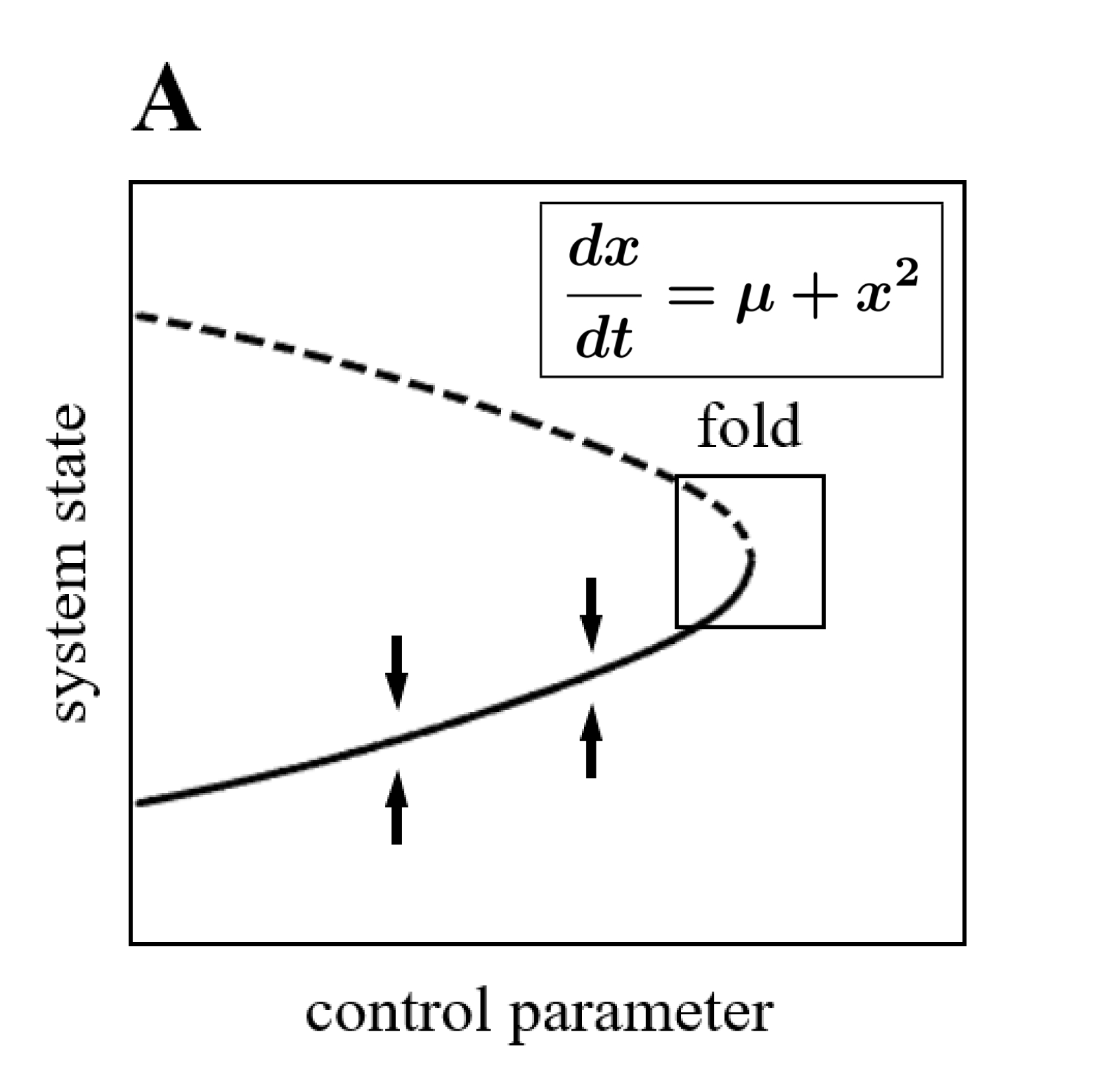
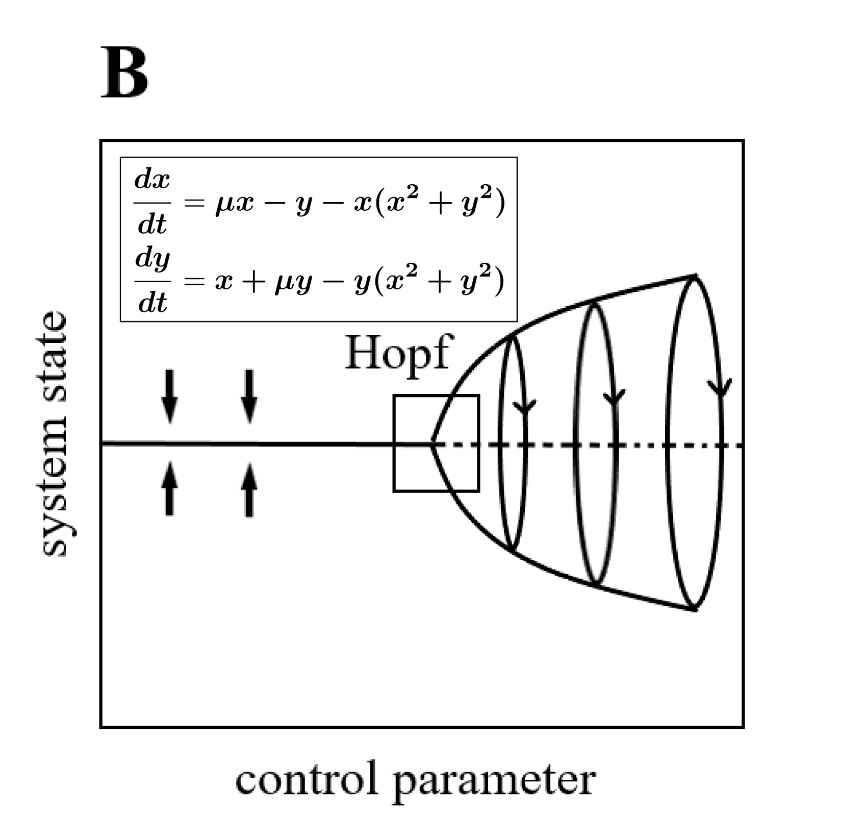
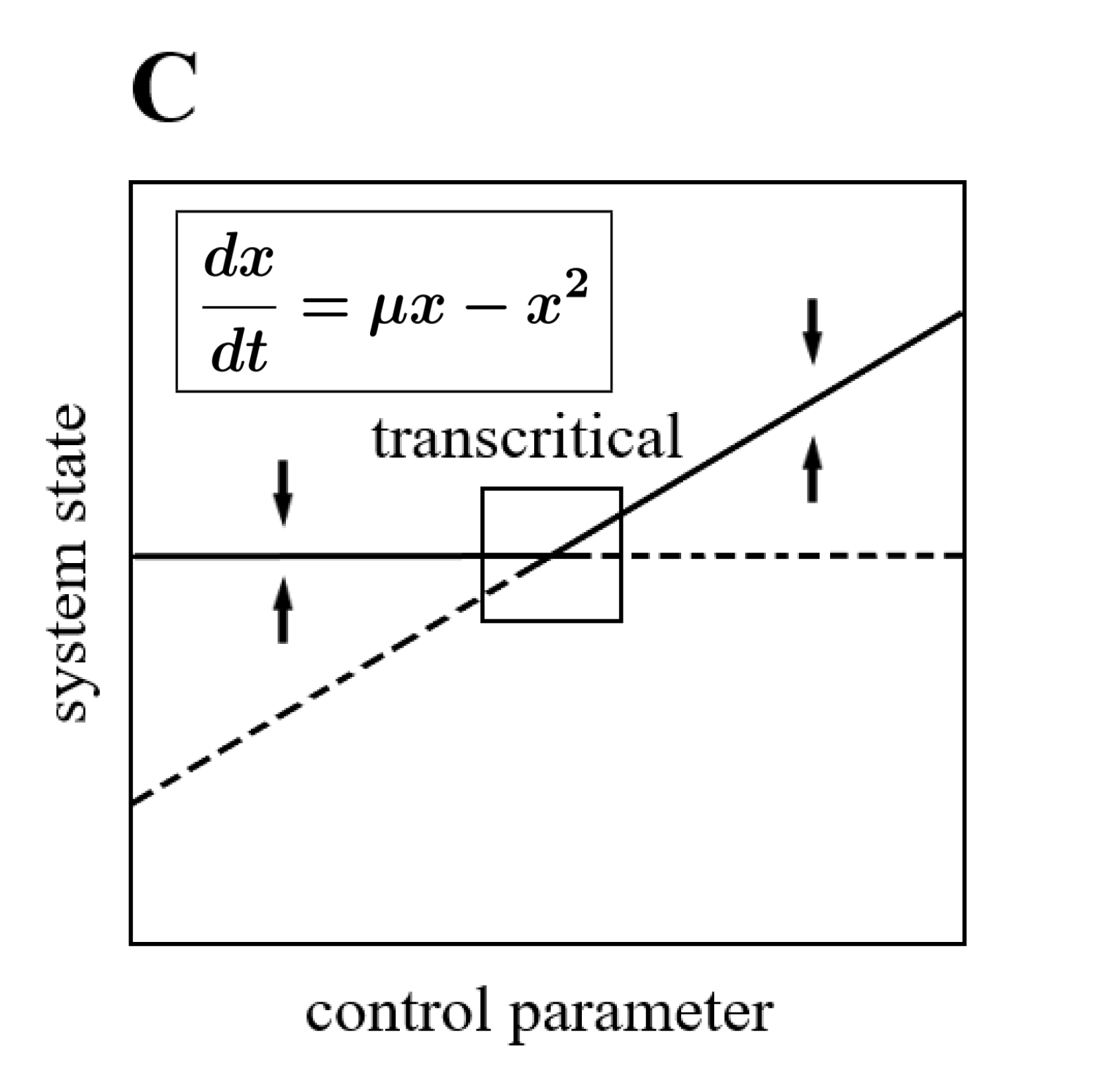
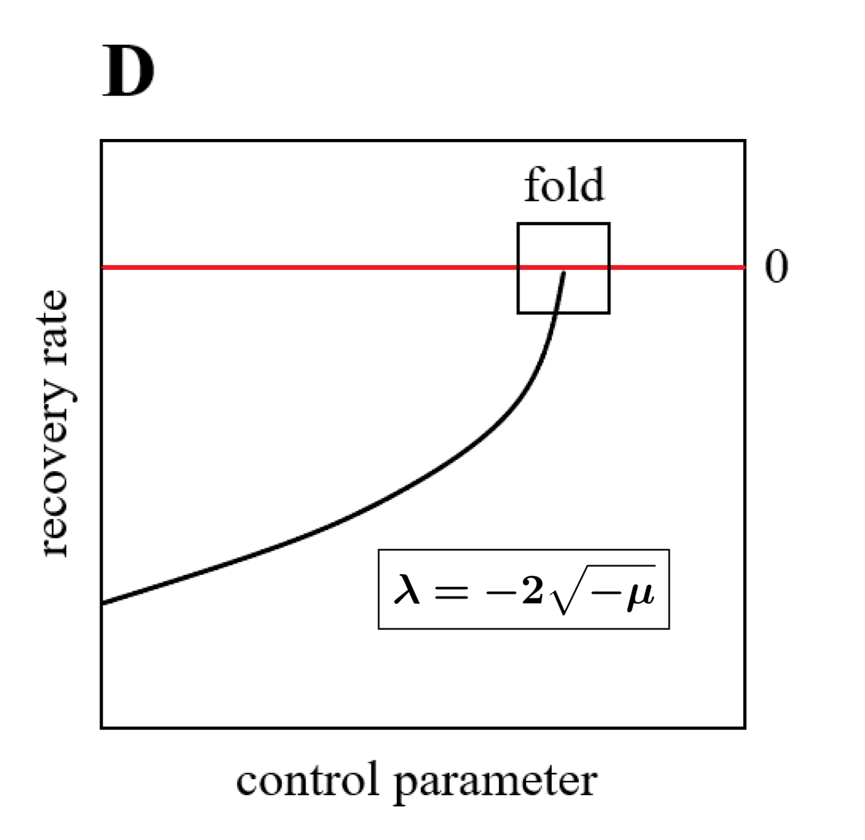
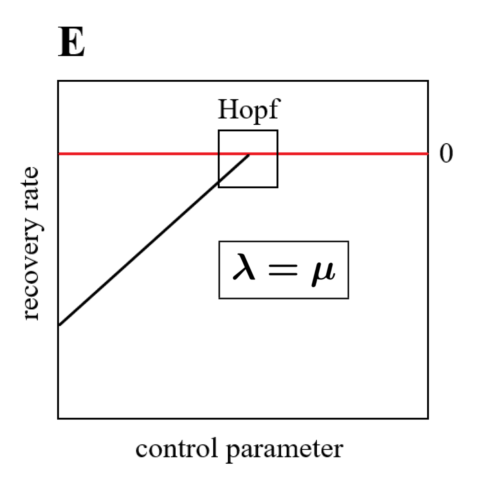
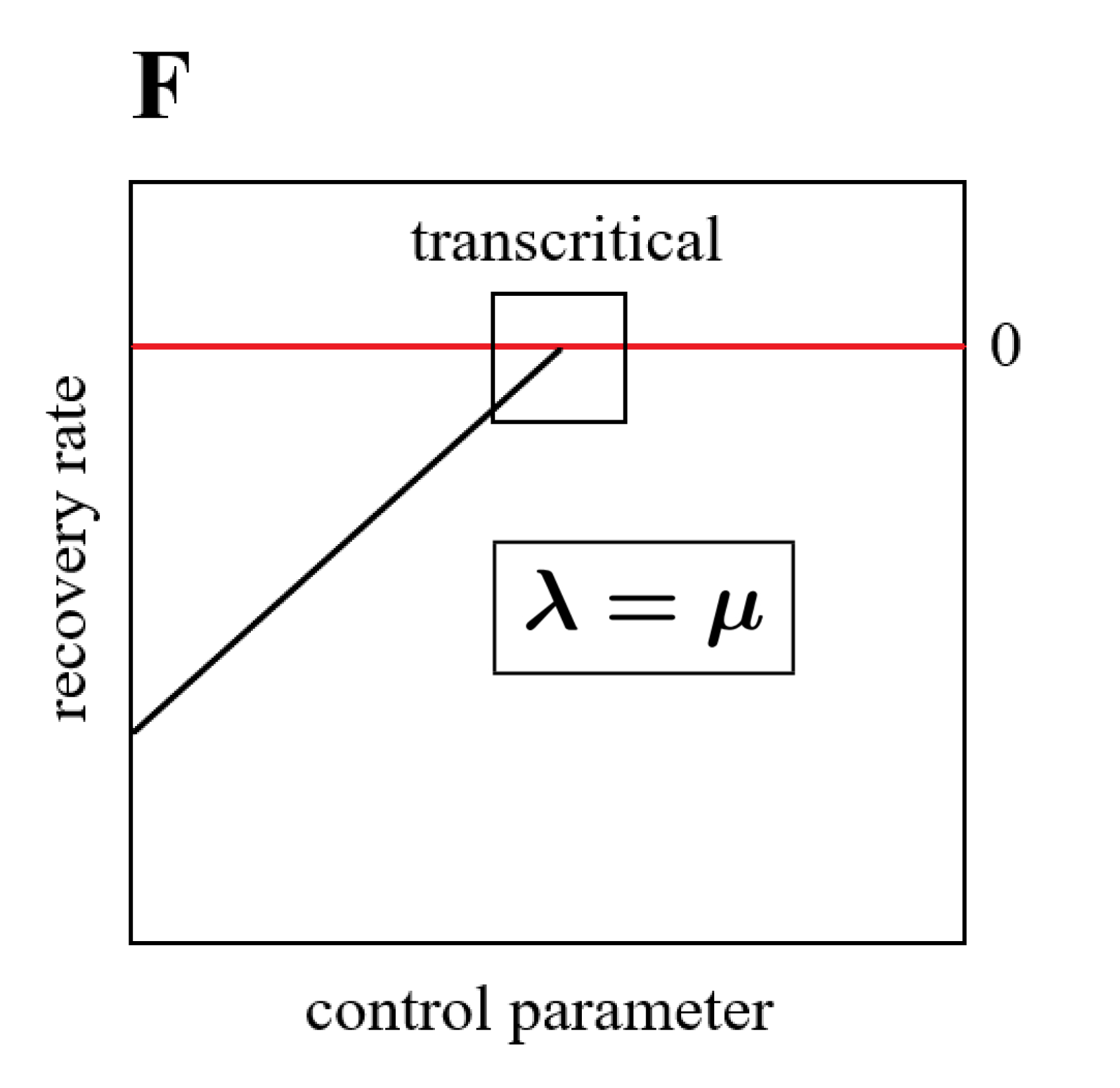
Fig.1   (A-C) The normal forms of fold, (supercritical) Hopf, and transcritical bifurcation where bifurcation occurs at $\mu=0$ (hollow square). Their mathematical expressions are inside the boxes within the corresponding figures. (D-F) The recovery rate $\lambda$ of the normal forms for the fold, (supercritical) Hopf, and transcritical bifurcation as a function of the control parameter $\mu$, their function expressions are inside the boxes within the corresponding figures. Bifurcation occurs when the recovery rate $\lambda$ reaches zero (hollow square).

Performance of DL algorithm on model time series

We applied the DL model on regularly-sampled time series generated from three ecological models with white noise and three climate models with red noise. We generated test data with 11 different initial values of the bifurcation parameter for each model and 50 test time series for each initial value of the bifurcation parameter. To evaluate the performance of DL algorithm, we measured the relative error(25) of tipping points prediction for each of the 50 test time series associated with every initial value of the bifurcation parameter. The performance of DL algorithm is evaluated by the mean relative error of tipping points prediction, which is averaged over the 50 measurements of the relative error of tipping points prediction for each initial value of the bifurcation parameter. We first compared the results of DL algorithm with those of degenerate fingerprinting(9), DEV(12) and null model in three ecological models with white noise which exhibit fold, Hopf and transcritical bifurcations respectively. Then we compared the results of DL algorithm with those of BB method(10), DEV(12) and null model in three climate models with red noise which exhibit fold, Hopf and transcritical bifurcations respectively. As Fig. 2 shows, the DL algorithm outperforms the other competing algorithms for all initial values of each model. Moreover, the DL algorithm exhibits smaller fluctuations of relative error of tipping points prediction than the other competing algorithms for each initial value and exhibits smaller fluctuations of the mean relative error of tipping points prediction than the other competing algorithms across different initial values. Our results suggest that the DL algorithm is more robust against different initial values of the bifurcation parameter than competing algorithms.

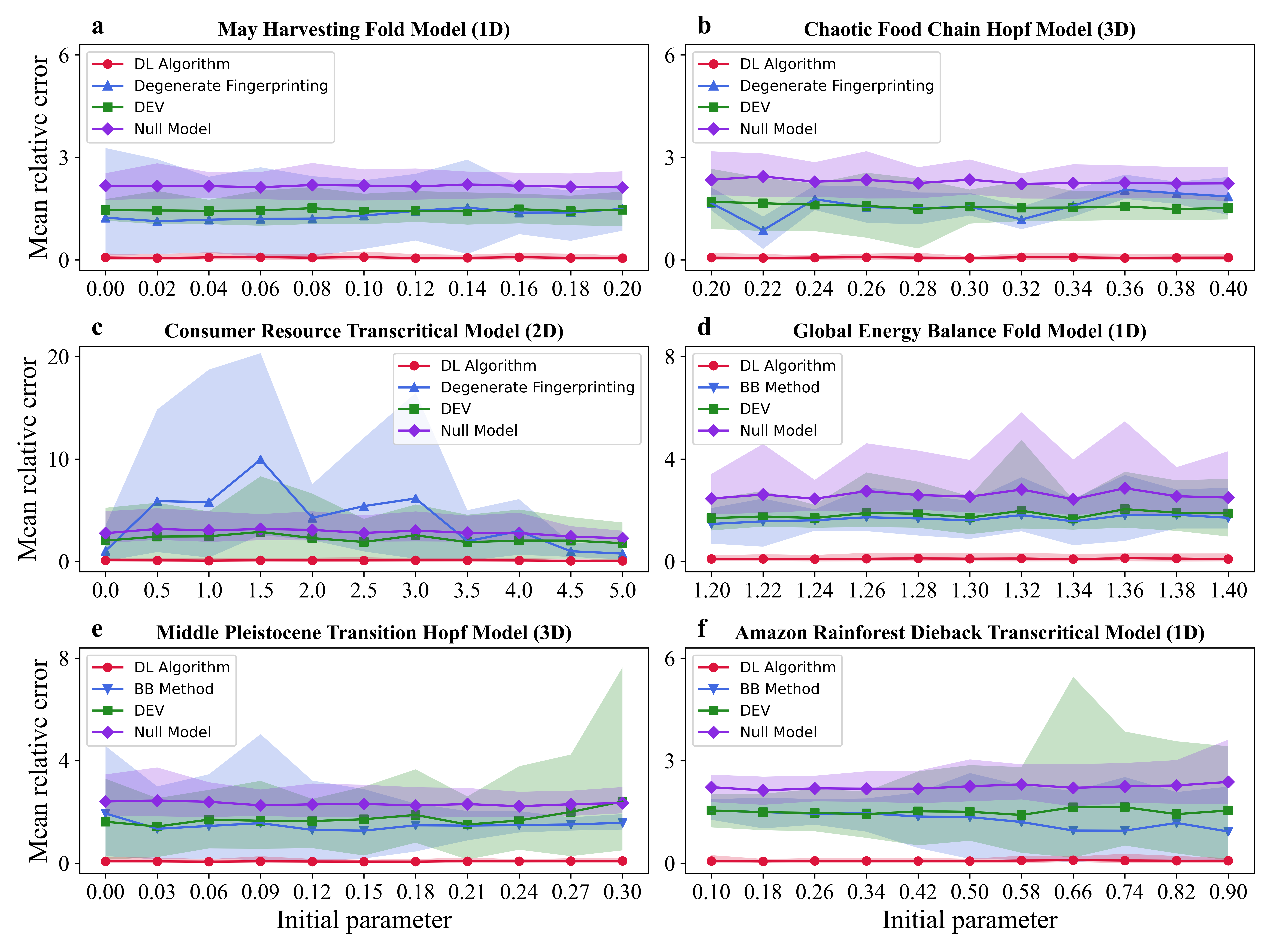
Fig.2   We tested the DL model on regularly-sampled model time series with 11 initial values of bifurcation parameter. Here the mean relative error of tipping points prediction is plotted as a function of initial parameter. The area covered by the polyline represents the 90% confidence interval for the relative error of tipping points prediction. (a-c) We compared the DL algorithm (red lines) with degenerate fingerprinting (blue lines), DEV (green lines) and null model (purple lines) on three ecological model time series with white noise. These model time series undergo fold, Hopf, and transcritical bifurcation, occurring at $0.268$, $0.480$, and $5.882$, respectively. (d-f) The DL algorithm (red lines) is compared with BB method (blue lines), DEV (green lines) and null model (purple lines) on three climate model time series with red noise. These model time series undergo fold, Hopf, and transcritical bifurcation, occurring at $0.962$, $0.355$, and $-0.005$, respectively.

We further tested the DL model on irregularly-sampled time series from the above six models. It is worth noting that the above competing algorithms are not applicable for irregularly-sampled time series. Therefore, we used linear interpolation to transform these irregularly-sampled time series into equidistant data. This allows us to use the competing algorithms of degenerate fingerprinting, BB method and DEV for detecting early warning signals on reconstructed model time series(42). The null model is also applied as a competing algorithm. From Fig. 3, we find that DL algorithm outperforms the other competing algorithms for all initial values of each model. Moreover, our results suggest that the DL algorithm is more robust against different initial values of the bifurcation parameter than competing algorithms.

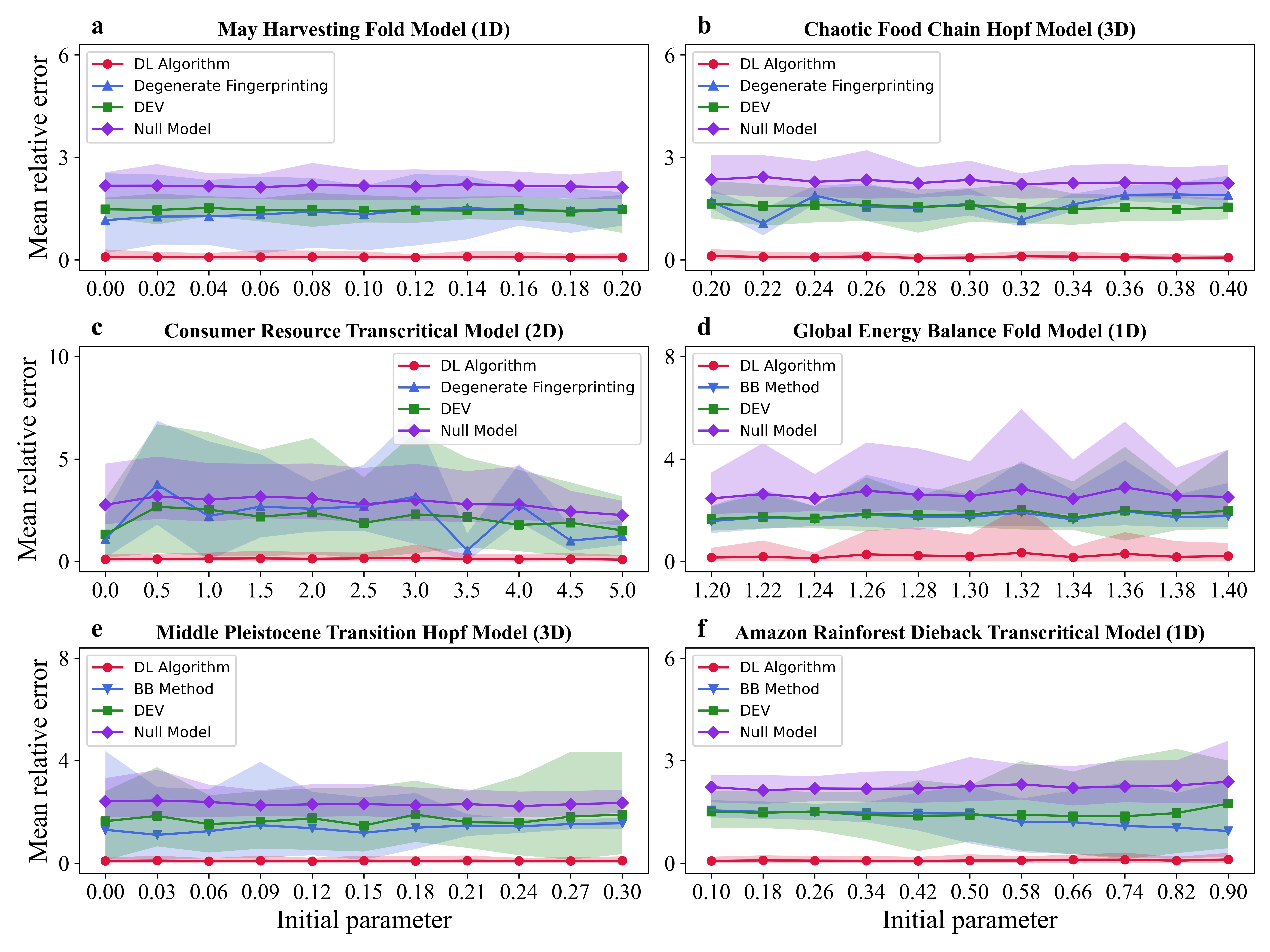
Fig.3   We tested the DL model on irregularly-sampled model time series with 11 initial values of bifurcation parameter. Here the mean relative error of tipping points prediction is plotted as a function of initial parameter. The area covered by the polyline represents 90% confidence interval for the relative error of tipping points prediction. (a-c) We compared the DL algorithm (red lines) with degenerate fingerprinting (blue lines), DEV (green lines) and null model (purple lines) on three ecological model time series with white noise. (d-f) The DL algorithm (red lines) is compared with BB method (blue lines), DEV (green lines) and null model (purple lines) on three climate model time series with red noise. We used linear interpolation to transform these irregularly-sampled time series into equidistant data so that they are suitable for degenerate fingerprinting, BB method and DEV.

We then tested the DL model on irregularly-sampled time series from the ascending arousal system with a fold/fold hysteresis loop. We conducted an irregular sampling of 400 points within the bifurcation parameter intervals of $[0.1,0.7]$ and $[1.3,1.9]$ (bifurcation parameter decreases in this interval) respectively. We applied the DL model on these irregularly-sampled time series and predicted that the tipping points occur at 1.157 and 0.877 with relative errors of tipping points prediction of 0.84% and 1.49% respectively, as shown in Fig. 4 (a). Similarly, we tested the DL model on irregularly-sampled time series from the Sprott B system with a Hopf/Hopf-hysteresis bursting. We irregularly sampled 400 points from the bifurcation parameter intervals of $[\pi,1.3\pi]$ and $[1.7\pi,2\pi]$ (bifurcation parameter decreases in this interval) respectively. We applied the DL model on these irregularly-sampled time series and predicted that the tipping points occur at $1.461\pi$ and $1.540\pi$ with relative errors of tipping points prediction of 0.05% and 0.81% respectively, as shown in Fig. 4 (b). Our results suggest that the DL algorithm is effective for tipping point prediction in theoretical models with hysteresis phenomenon.

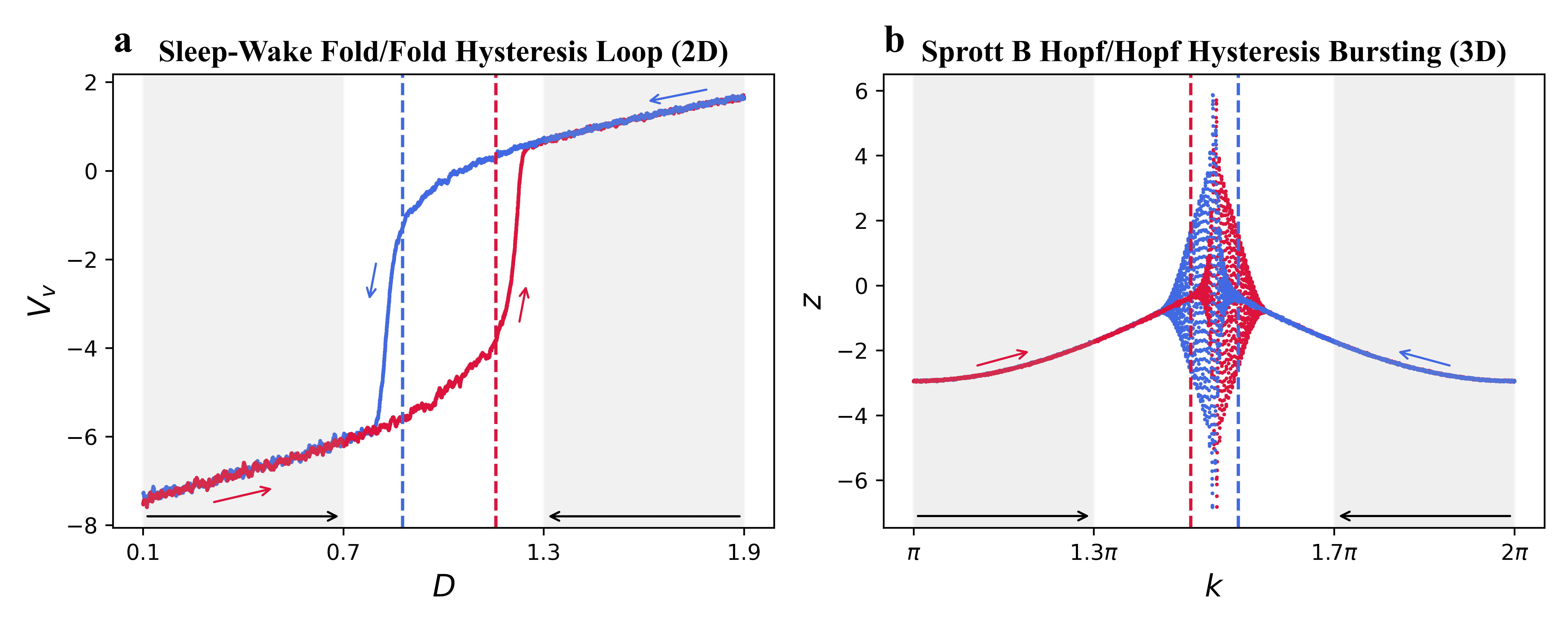
Fig.4   The performance of the DL algorithm in predicting transitions of irregularly-sampled time series generated by theoretical models exhibiting hysteresis. The red and blue curves illustrate the time series forced by increasing and decreasing bifurcation parameter respectively, while the grey area denotes the range of time series data used for prediction. (a) In the case of the sleep-wake system, a fold/fold hysteresis loop is observed at $D=1.152$ and $D=0.883$. The predicted tipping points are $1.157$ (red dashed line) and $0.877$ (blue dashed line) respectively. (b) For the Sprott B system, a Hopf/Hopf hysteresis bursting occurs at $k=1.461\pi$ and $k=1.539\pi$. The predicted tipping points are $1.461\pi$ (red dashed line) and $1.540\pi$ (blue dashed line) respectively.

Performance of DL algorithm on empirical time series

We tested the DL model on three empirical examples, including a cyanobacteria microcosm experiment under light stress(37), a physical experiment of voice oscillation during heat(20) and metallic elements concentration in sediment cores collected from the eastern Mediterranean Sea(38). For each empirical system, we applied the DL model to four irregularly-sampled time series, each containing 400 data points, across different parameter ranges. Then we used linear interpolation to transform these irregularly-sampled records to time series with equidistant data. This allows us to use the competing algorithms of degenerate fingerprinting, BB method and DEV for detecting early warning signals on reconstructed empirical records(42). Note that the first two empirical examples from ecology and physics are subject to white noise while the third empirical example from paleoclimatology is subject to red noise(43). Therefore, we applied degenerate fingerprinting to the first two empirical examples and BB method to the third empirical example. We compared the results of the DL algorithm with those of four competing algorithms, including degenerate fingerprinting, BB method, DEV and null model.

In the cyanobacteria microcosm experiment under light stress, the photo-inhibition drives a cyanobacterial population, measured by light attenuation coefficient, towards a tipping point with fold bifurcation when a critical threshold of light irradiance is approached(37). To validate our DL algorithm, we applied the DL model to the empirical time series sampled in four periods which are from day 1 to day 16, from day 1.5 to day 16.5, from day 2 to day 17 and from day 2.5 to day 17.5 respectively. The corresponding range of bifurcation parameter of light irradiance for the four periods is from 477 to 845$\rm\mu$mol photons $\rm m^{-2}s^{-1}$, from 488.5 to 856.5$\rm\mu$mol photons $\rm m^{-2}s^{-1}$, from 500 to 868$\rm\mu$mol photons $\rm m^{-2}s^{-1}$, and from 511.5 to 879.5$\rm\mu$mol photons $\rm m^{-2}s^{-1}$ respectively. The corresponding tipping points predicted by the DL model are 1088.5$\rm\mu$mol photons $\rm m^{-2}s^{-1}$, 1090.9$\rm\mu$mol photons $\rm m^{-2}s^{-1}$, 1088.2$\rm\mu$mol photons $\rm m^{-2}s^{-1}$, and 1090.4$\rm\mu$mol photons $\rm m^{-2}s^{-1}$ respectively, which are all very close to 1091$\rm\mu$mol photons $\rm m^{-2}s^{-1}$, the true value of the tipping point. From Fig. 5 A1-A4, we find that the DL algorithm outperforms the other competing algorithms in all cases. These results suggest the robustness of the DL algorithm in tipping points prediction against different light irradiance intervals.

The second empirical data we analyzed is the thermoacoustic system. The state of the thermoacoustic system is measured by acoustic pressure. The thermoacoustic system undergoes a Hopf bifurcation from a non-oscillatory to an oscillatory state with increasing voltage(24, 44, 45, 46). It has also been demonstrated that the transition to high amplitude limit cycle oscillations occurs later for faster changing rate of voltage, which can be explained by rate-delayed tipping(20, 21). In order to verify the robustness of DL algorithm in tipping points prediction against different changing rates of voltage, we applied the DL model to empirical time series under three voltage changing rates (20mV/s, 40mV/s, 60mV/s) within the bifurcation parameter voltage ranges from 0 to 1 V, from 0.05 to 1.05 V, from 0.1 to 1.1 V and from 0.15 to 1.15V respectively. From Fig. 5 B1-B4, we find that the DL algorithm outperforms the other competing algorithms in predicting the tipping points, where the acoustic pressure starts to oscillate, for various voltage intervals of empirical data under the voltage changing rate of 20mV/s. We further test these algorithms for different changing rates of voltage as shown in Supplementary Fig. 16, which suggest the DL algorithms also shows best performance among all these algorithms. These results suggest that the DL algorithm is robust against various voltage intervals and changing rages of voltage.

The third empirical data is the concentration of metallic elements in sediment cores collected from the eastern Mediterranean Sea. The concentration of metallic elements changes rapidly due to the transition between oxic and anoxic states occurred regularly in this region. The bifurcation types of these transitions have been uncovered by previous study(18). We studied the Mo concentration in sediment cores and the U concentration in sediment cores collected in different periods of time, which are from 160 to 125 ka BP and from 300 to 240 ka BP respectively. We lacked information on the bifurcation parameter series data in this example, therefore we used age as a substitute for the bifurcation parameter. Since the Mo concentration in sediment cores undergoes fold bifurcation, we applied the DL model on this data within four age intervals, from 160 to 140 ka BP, from 159 to 139 ka BP, from 158 to 138 ka BP and from 157 to 137 ka BP respectively. However, the U concentration in sediment cores undergoes transcritical bifurcation. We applied the DL model on this data within four age intervals, from 300 to 268 ka BP, from 298 to 266 ka BP, from 296 to 264 ka BP and from 294 to 262 ka BP respectively. We find that the DL algorithm outperforms the other competing algorithms in predicting tipping points where the concentration of metallic elements Mo or U in sediment cores change dramatically for various age intervals of empirical data as shown in Fig. 5 C1-C4 and Fig. 5 D1-D4. These results also suggest the robustness of the DL algorithm in tipping points prediction against various age intervals.

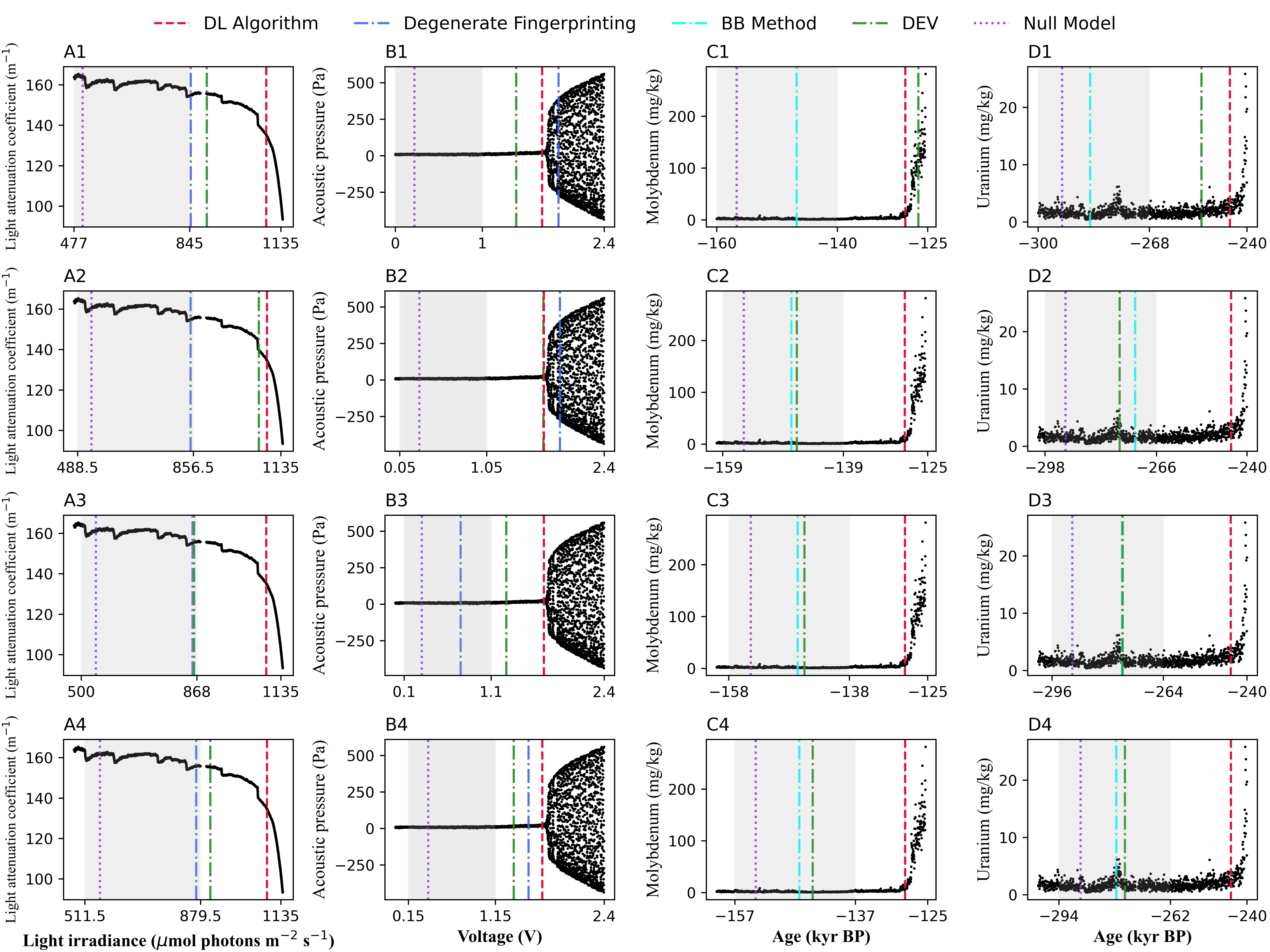
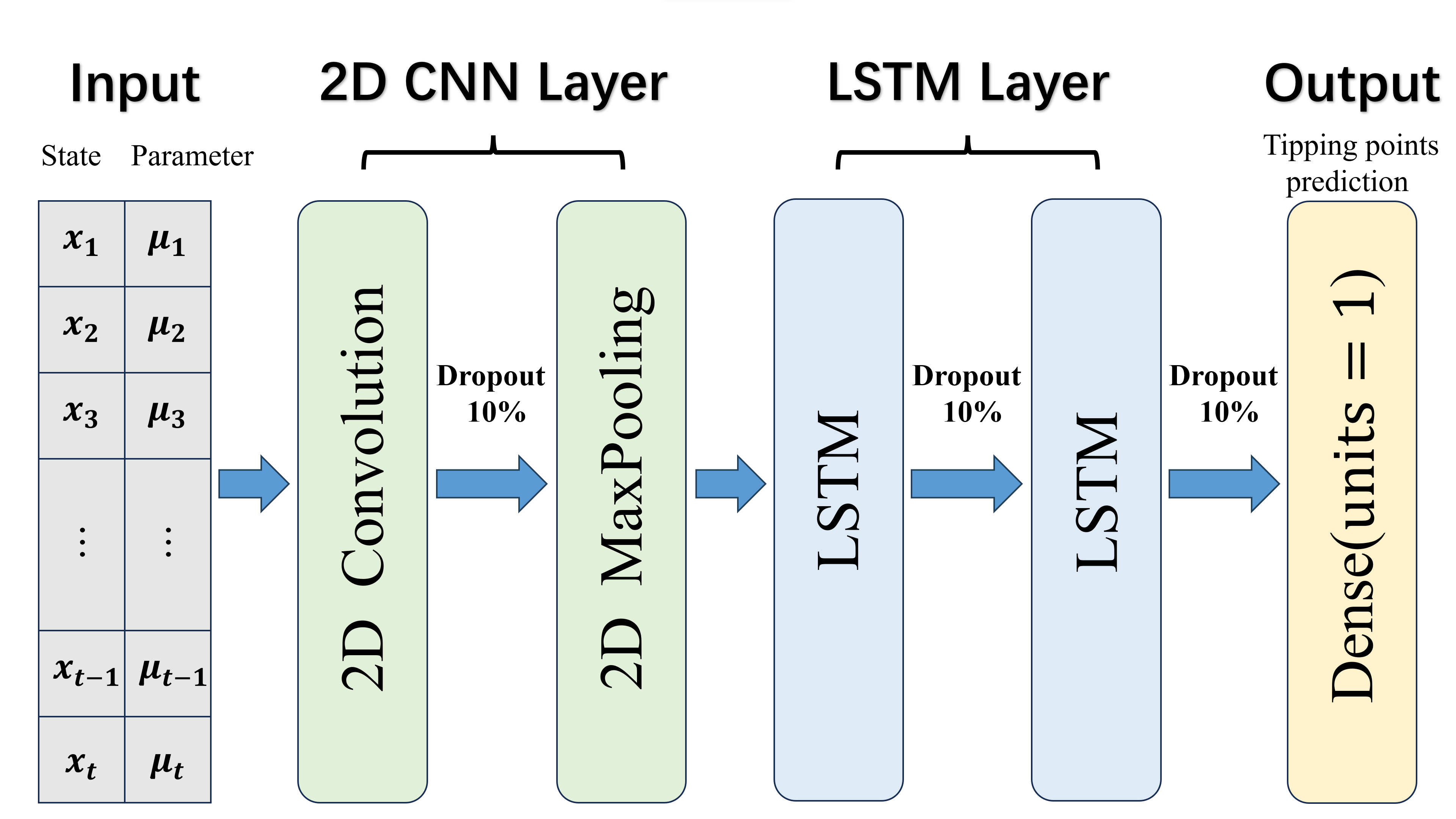
Fig.5   The performance of DL algorithm in predicting tipping points on irregularly-sampled empirical time series. Grey region represents the range of empirical time series used for prediction. (A1-A4) Cyanobacterial population undergoes a fold bifurcation, which is measured by light attenuation coefficient. (B1-B4) The thermoacoustic system undergoes a Hopf bifurcation under the 20mV/s changing rate of the control parameter voltage. (C1-C4) The eastern Mediterranean Sea experienced an anoxic event, it exhibited a fold bifurcation, which was measured using the concentration of Mo in sediment cores. (D1-D4) The eastern Mediterranean Sea experienced another anoxia event, characterized by a transcritical bifurcation, which was measured using the concentration of U in sediment cores. We compared the performance of the DL algorithm (red dashed lines) with degenerate fingerprinting (blue dash-dot lines), BB method (cyan dash-dot lines), DEV (green dash-dot lines) and null model (purple dotted lines). We used linear interpolation to transform these irregularly-sampled time series into equidistant data so that they are suitable for degenerate fingerprinting, BB method and DEV.

Fig.6   The 2D CNN-LSTM architecture. The 2D convolutional kernel processes state series and bifurcation parameter series into one-dimensional local feature series. These features are then subjected to local max pooling, followed by analysis using an LSTM layer. Finally, the features processed by the LSTM are mapped to the prediction of tipping point, through a fully connected layer.

Discussion

Predicting the occurrence of tipping points based on time series is a challenging problem. In this work, we develop a deep learning algorithm that exploits information of normal form from the training systems for tipping points prediction. This algorithm can deal with both regularly-sampled and irregularly-sampled time series. Our results show that the DL algorithm not only outperforms traditional methods in the accuracy of tipping points prediction for regularly-sampled time series, but also achieve accurate prediction for irregularly-sampled time series. Our results pave the way to make effective strategies to prevent and prepare tipping points from various real-world systems(47).

There are three major advantages of our work. First, traditional methods for tipping points prediction can only deal with regularly-sampled time series(9, 10, 11, 12). However, the DL algorithm used in this paper can deal with both regularly-sampled time series and irregularly-sampled time series. This is because the bifurcation parameter series input into the 2D CNN layer contains the information about the sequence of distance between adjacent points, which is used for tipping points prediction. Second, the effect of rate-delayed tipping has been ignored in previous methods for tipping points prediction(9, 10, 11, 12). This is due to the limitations of the theory of fast-slow systems used in previous methods. However, we consider the effect of rate-delayed tipping in our work and label the data by using the fact that the quasi-static attractor loses stability at the occurrence of tipping points in our training set (see Methods for details). The DL algorithm trained with such labels is robust against different changing rates of bifurcation parameter (Supplementary Fig. 16). Third, previous methods for tipping points prediction require test data that includes samples taken near the tipping points where pronounced early warning signals are present, particularly for the bifurcation theory based methods(9, 12). However, most of the time series from our experiments were sampled beyond a certain distance from the tipping points, leading to the unsuccessful performance of these algorithms in predicting tipping points shown in this paper. The DL algorithm, in contrast, can accurately identify the location where the tipping points occur with various distance between the end of the time series and the tipping points.

Most previous methods require full information of all interacting variables in the dynamical systems for predicting tipping points, such as the time series of interacting variables(9, 48). However, this information is often not available especially for large systems. Therefore, it is often not feasible to use those methods for predicting tipping points of real-world systems. In this work, we use time series of only a single variable in the dynamical system as prior information for predicting tipping points. Such time series is commonly available from real-world systems, because it is very likely that only one or few variables in the systems are measured(12). The theoretical foundation of our algorithm lies in Takens embedding theorem(13). Specifically, the time series of a single variable preserves dynamical information of the entire system, which can provide sufficient information for tipping points prediction.

Our work raises several problems worthy of future pursuit. First, we have studied the situation of local codimension-one bifurcations in continuous-time dynamical systems in this paper. For future work, we can focus on tipping points prediction in discrete-time dynamical systems, such as period-doubling bifurcation(7) which arise naturally in physiology(49, 50) and ecology(51). It would be interesting to develop a method that can deal with both regularly-sampled and irregularly-sampled time series for systems with period-doubling bifurcation. Second, it would be interesting to investigate tipping points prediction in systems with other types of bifurcation, such as codimension-two bifurcation and global bifurcation(7). Yet, tipping points prediction in systems with codimension-two bifurcation and global bifurcation are more challenging than that in systems with codimension-one bifurcation. Third, one can develop interpretable machine learning models for tipping points prediction by combing dynamical system theory with neural networks(52, 53, 54, 55, 56), which offer an avenue for making safe and reliable high-stakes decisions for policy makers(57).

Methods

Generation of training data for the DL algorithm

We construct two-dimensional dynamical systems of the following form which are used to generate the training data based on simulation(18)

$$\frac{dx}{dt}=\sum_{i=1}^{10}a_{i}p_{i}(x,y)$$ (1)

$$\frac{dy}{dt}=\sum_{i=1}^{10}b_{i}p_{i}(x,y),$$

where $x$ and $y$ are state variables, $p(x,y)$ is a vector containing all polynomials in $x$ and $y$ from zero up to third order

$$p(x,y)=(1,x,y,x^{2},xy,y^{2},x^{3},x^{2}y,xy^{2},y^{3}),$$

$p_{i}(x,y)$ is the $i$-th component of $p(x,y)$. $a_{i}$ and $b_{i}$ are parameters randomly drawn from standard normal distribution, and then, half of these parameters are selected at random and set to zero. The parameters for the cubic terms are set to the negative of their absolute values to encourage models with bounded solutions. Since our training data is required to contain representation of all possible dynamics that may occur in the study time series data, we generate models with different sets of parameter values in Eqs. 1 until a required number of each type of bifurcation (fold, Hopf, or transcritical) has been discovered. We add white or red noise to these models to simulate training data for the DL algorithm.

After a model is generated, we perform numerical simulation of this model with 10,000 time steps from a randomly drawn initial condition and test whether the system converges to an equilibrium point. The odeint function from the Python package Scipy(58) is applied in the numerical simulation with a step size of 0.01. The criteria that we used to determine the convergence is that the maximum difference between the final 10 points in numerical simulation is less than $10^{-8}$. The convergence is required in order to search for bifurcations which occur at non-hyperbolic equilibria(7). The models that do not converge are discarded. For the models that converge, we apply AUTO-07P(59) to identify bifurcations along the equilibrium branch by either increasing or decreasing each nonzero parameter. For each bifurcation identified, we first set the initial condition with the value of the equilibrium of the model and a burn-in period of 100 units of time. Then we run simulations of the model with noise and obtain the quasi-static attractor time series with noise and bifurcation parameter time series which are used for training. We also run simulations of the same model without noise and obtain the corresponding quasi-static attractor time series and bifurcation parameter time series which are used for calculating the recovery rate $\lambda$ to locate the bifurcation point where $\lambda$ changes from negative value to positive value,

$$\lambda=max(Re(eigvals(\begin{bmatrix}\frac{\partial(\sum_{i=1}^{10}a_{i}p_{i}(x,y))}{\partial x}&\frac{\partial(\sum_{i=1}^{10}a_{i}p_{i}(x,y))}{\partial y}\\ \frac{\partial(\sum_{i=1}^{10}b_{i}p_{i}(x,y))}{\partial x}&\frac{\partial(\sum_{i=1}^{10}b_{i}p_{i}(x,y))}{\partial y}\end{bmatrix}_{(x,y)=(x^{*},y^{*})}))).$$ (2)

The simulations of the models with noise are based on the Euler Maruyama method(60) with a step size of 0.01 and the simulations of the models without noise are based on Euler method(61) with the same step size.

For each model where a bifurcation is identified, we perform five independent simulations of the model with varying bifurcation parameter from its initial value to a terminal value beyond the bifurcation point given by AUTO-07P. In these five simulations, we set the changing rate of the bifurcation parameter to remain constant within each simulation where the changing rate of the bifurcation parameter is the change in the bifurcation parameter per unit time with a step size of 0.01, but vary across different simulations. The ratio of each changing rate of the bifurcation parameter to the smallest changing rate of the bifurcation parameter in these five simulations is drawn from 1, 2, …, 10. The nonzero changing rate of the bifurcation parameter can lead to the delay in the occurrence of tipping points, which is called rate-delayed tipping(20, 21). Due to rate-delayed tipping, the theoretical bifurcation point given by AUTO-07P is not the accurate location of the tipping point. Therefore, we identify the location of the tipping point by the recovery rate (Eq. 2) and use this identified tipping point as the training label for our supervised deep learning training process (Supplementary Information section 2.3). If no tipping point is detected in a simulation, this simulated data will be discarded. Otherwise, we randomly and irregularly sample $l_{s}$ points from quasi-static attractor time series with noise which is simulated by the variable $x$ of the model and corresponding bifurcation parameter time series between the initial value and the tipping point, where $l_{s}$ is drawn from $Uniform(505,1000)$. Then we select the first 500 points as training data. The obtained training data can make DL algorithm to learn the features of recovery rate from time series data with different changing rates of parameter and varying distances between the end of the time series and the tipping points.

Here we train deep learning algorithm on datasets with white and red noise. The white noise in simulation has the amplitude drawn from a triangular distribution centered at 0.01 with upper and lower bounds 0.0125 and 0.0075 respectively while the red noise is modeled by AR(1) process in which the lag-1 autoregressive coefficient is between -1 and 1. It is worth noting that the simulations shift to new regime before the bifurcation point due to the noise(62, 63). Since the location of this premature transition is stochastical, we still use the location where the quasi-static attractor without noise loses stability as the training label for DL algorithm even it is not accurate. We mathematically illustrate how slight perturbation causes bifurcation to occur earlier and its stochasticity in Supplementary Information section 6.

DL algorithm architecture and training

In this paper we use the 2D CNN-LSTM DL algorithm(64, 65). The 2D CNN-LSTM architecture is shown in Fig. 6. We use a train/validation/test split of 0.95/0.04/0.01 for the DL algorithm, and MSE as the loss function to minimize the difference between the real tipping points (training labels) and the predictions. The DL algorithm is trained on 300,000 instances for 200 epoches. We train ten neural networks and report the performance of the DL algorithm averaged over them. The hyperparameters of the DL model are tuned through random search, and we present the optimal hyperparameters of the DL model in Supplementary Table 1.

Before training our DL algorithm, there are several preprocessing matters(66). The quasi-static attractor time series with noise are detrended using Lowess smoothing with a span of 0.2 to obtain the residual time series used for training. Besides, in order to obtain the robustness of DL algorithm on time series of various lengths, we zero out the left side of the residual time series and corresponding bifurcation parameter time series, with the length drawn from $Uniform(0,250)$. Due to the zeroing process, the DL algorithm can deal with time series even if it is a little short. After the zeroing process, each residual time series is normalized by dividing each time series data point by the average absolute value of the residuals across the non-zero part of the time series. In addition, each bifurcation parameter time series is also normalized: each data point in the time series minus the initial value of the bifurcation parameter time series, and then divided by the distance between the initial and final values of the bifurcation parameter time series, thereby mapping the bifurcation parameter time series to the interval of $[0,1]$. The corresponding label, i.e., the tipping point, is normalized following the same procedure as the normalization of the data point in bifurcation parameter time series. Thus the relative distance of tipping point to the time series in the training set for the DL algorithm (calculated as the tipping points minus the final value of the bifurcation parameter time series, divided by the distance between the initial and final values of the bifurcation parameter time series) is between 0.01 and 2. In other words, the labels in the training set, after normalization, will fall within the interval of $[1.01,3]$.

Theoretical models used for testing

The simulation of theoretical models with noise is based on the Euler Maruyama method(60) with a step size of 0.01 ($\delta t=0.01$ units of time) unless otherwise stated. The amplitude of white noise $\sigma$ is 0.01 while the red noise is modeled by AR(1) process in which the lag-1 autoregressive coefficient $\phi$ is drawn from $Uniform(-1,1)$. We fix the changing rate of the bifurcation parameter in each simulation of the same theoretical model to ensure that these simulations have the same bifurcation point. The bifurcation point of each simulation is the location where the recovery rate changes from negative value to positive value. Then we sample from these simulations to obtain regularly-sampled model time series and irregularly-sampled model time series for testing. The lengths of these model time series range from 250 to 500, and the relative distances of tipping points to these time series range from 0.01 to 2.

We apply the relative error $\varepsilon$ of tipping points prediction to evaluate the performance of the DL algorithm, which is defined as

$$\varepsilon=\frac{\left|\widehat{\mu}_{c}-\mu_{c}\right|}{\left|\mu_{end}-\mu_{c}\right|},$$

where $\widehat{\mu}_{c}$ is the predicted tipping point, $\mu_{c}$ is the real tipping point, $\mu_{end}$ is the value of bifurcation parameter for last point of the test time series.

Theoretical models with white noise

To test the fold bifurcation with white noise, we use the May’s harvesting model(28). This is given by

$$\frac{dx}{dt}=rx(1-\frac{x}{k})-\frac{hx^{2}}{s^{2}+x^{2}}+\sigma\xi(t),$$

where $x$ is biomass of some population, $k$ is its carrying capacity, $h$ is the harvesting rate, $s$ characterizes the nonlinear dependence of harvesting output on current biomass, $r$ is the intrinsic per capita growth rate of the population, and $\xi(t)$ is a Gaussian white noise process. We use parameter values $r=1$, $k=1$, $s=0.1$ and $h$ increases at a rate of $6.25\times 10^{-4}$. We generate model time series by this equation from eleven initial values of $h$, which are $0,0.02,0.04,...,0.18,0.2$. In this configuration, a fold bifurcation occurs at $h=0.268$ (Supplementary Fig. 9).

To test the Hopf bifurcation with white noise, we use a three-species chaotic food chain model(29). This is given by

$$\frac{dr}{dt}=r(1-\frac{r}{k})-\frac{x_{c}y_{c}cr}{r+r_{0}}+\sigma\xi_{r}(t),$$

$$\frac{dc}{dt}=x_{c}c(\frac{y_{c}r}{r+r_{0}}-1)-\frac{x_{p}y_{p}pc}{c+c_{0}}+\sigma\xi_{c}(t),$$

$$\frac{dp}{dt}=x_{p}p(\frac{y_{p}c}{c+c_{0}}-1)+\sigma\xi_{p}(t),$$

where $r$, $c$, and $p$ are the population densities of the resource, consumer, and predator species, respectively. $k$ is a parameter characterizing the environmental capacity of the resource species. $x_{c}$, $y_{c}$, $x_{p}$, $y_{p}$, $r_{0}$, and $c_{0}$ are other parameters in the system. $\xi_{r}(t)$, $\xi_{c}(t)$ and $\xi_{p}(t)$ are independent Gaussian white noise processes. For our simulations, we use parameter values $x_{c}=0.4$, $y_{c}=2.009$, $x_{p}=0.08$, $y_{p}=2.876$, $r_{0}=0.16129$, $c_{0}=0.5$ and $k$ increases at a rate of $1.54\times 10^{-3}$. We generate model time series by these equations from eleven initial values of $k$, which are $0.20,0.22,0.24,...,0.38,0.40$. In this configuration, a Hopf bifurcation occurs at $k=0.480$ (Supplementary Fig. 10).

To test the transcritical bifurcation with white noise, we use the Rozenzweig-MacArthur consumer-resource model(30). This is given by

$$\frac{dx}{dt}=gx(1-\frac{x}{k})-\frac{axy}{1+ahx}+\sigma\xi_{x}(t),$$

$$\frac{dy}{dt}=\frac{eaxy}{1+ahx}-my+\sigma\xi_{y}(t),$$

where $x$ and $y$ are the population densities of the resource, consumer, respectively. $g$ is the intrinsic per capita growth rate of $x$, $k$ is its carrying capacity, $a$ is the attack rate of $y$, $e$ is the conversion factor, $h$ is the handling time, $m$ is the per capita consumer mortality rate, $\xi_{x}(t)$ and $\xi_{y}(t)$ are independent Gaussian white noise processes. We fix the parameter values $r=4$, $k=1.7$, $e=0.5$, $h=0.15$, $m=2$ and $a$ increases at a rate of $8.112\times 10^{-3}$. We generate model time series by these equations from eleven initial values of $a$, which are $0,0.5,1.0,...,4.5,5.0$. In this configuration, the system has a transcritical bifurcation at $a=5.882$ (Supplementary Fig. 11).

Theoretical models with red noise

To test the fold bifurcationn with red noise, we use a climate model describing temperature of an ocean on a spherical planet subjected to radiative heating(32, 31) which can simulate a transition from a greenhouse to an icehouse Earth(42). The model is given by

$$\frac{dT}{dt}=\frac{-e\rho T^{4}+\frac{1}{4}uI_{0}(1-a_{p})}{c}+\eta(t),$$

$$\text{with}\quad a_{p}=a-bT,$$

where $T$ is the average temperature of ocean, $u$ is relative intensity of solar radiation, $e$ is effective emissivity, $I_{0}$ is solar irradiance, $c$ is a constant thermal inertia, and $a_{p}$ is the planetary albedo. Parameters $a$ and $b$ define a linear feedback between ice and albedo variability and temperature. $\eta(t)$ is a red noise process with lag-1 autoregressive coefficient $\phi$. We use $e=0.69$, $I_{0}=71944000$, $c=10^{8}$, $a=2.8$, $b=0.009$, $\rho=0.03$, $\delta t=1$ time unit and $u$ decreases at a rate of $6\times 10^{-7}$. We generate model time series by this equation from eleven initial values of $u$, which are $1.4,1.38,1.36,...,1.22,1.2$. In this configuration, a fold bifurcation occurs at $u=0.962$ (Supplementary Fig. 12).

To test the Hopf bifurcation with red noise, we use the middle Pleistocene transition system(33), explaining the dynamics of glacial cycles, which is given by

$$\frac{dx}{dt}=-x-y+\eta_{x}(t),$$

$$\frac{dy}{dt}=-pz+uy+sz^{2}-yz^{2}+\eta_{y}(t),$$

$$\frac{dz}{dt}=-q(x+z)+\eta_{z}(t),$$

where $x$ represents the global ice volume, $y$ represents the atmospheric greenhouse gas concentration and $z$ represents a deep ocean temperature. All variables are rescaled to dimensionless form, $p=1$, $q=1.2$, $s=0.8$ are parameters, and $u$ increases at a rate of $8.4\times e^{-6}$. $\eta_{x}(t)$, $\eta_{y}(t)$ and $\eta_{z}(t)$ are independent red noise processes with lag-1 autoregressive coefficient $\phi$. We generate model time series by these equations from eleven initial values of $u$, which are $0,0.03,0.06,...,0.27,0.3$. In this configuration, a Hopf bifurcation occurs at $u=0.355$ (Supplementary Fig. 13).

To test the transcritical bifurcation with red noise, we use the simplified version of TRIFFID dynamic global vegetation model(34, 67). It can be used to simulate the dieback of the Amazon rainforest(67), which is mainly driven by climate change(68). The model is given by

$$\frac{dV}{dt}=PV^{*}(1-V)-GV+\eta(t),$$

where $V$ is equal to the broadleaf fraction, $G$ is a disturbance coefficient (0.004/year) and $V^{*}$ is either the value of $V$ or 0.1 if $V$ falls below 0.1. $\eta(t)$ is a red noise process with lag-1 autoregressive coefficient $\phi$. $P$ is the productivity, in dimensionless area fraction units, it decreases at a rate of $2.4\times 10^{-3}$. We generate model time series by this equation from eleven initial values of $P$, which are $0.90,0.82,0.74,...,0.18,0.10$. A transcritical bifurcation occurs at $P=-0.005$ in this configuration (Supplementary Fig. 14).

Theoretical models with hysteresis phenomenon

We also test our DL model on irregularly-sampled model time series generated by two theoretical neuroscience models with white noise. These systems exhibit hysteresis, which suggests that when the bifurcation parameter changes in opposite directions, these system will undergoes sudden shifts at different bifurcation points. The ascending arousal system is modeled in terms of the neuronal populations and their interactions(35), which is given by

$$\tau_{v}\frac{dV_{v}}{dt}=-V_{v}+v_{vm}Q_{m}+D+\sigma\xi_{v}(t),$$

$$\tau_{m}\frac{dV_{m}}{dt}=-V_{m}+v_{ma}Q_{a}+v_{mv}Q_{v}+\sigma\xi_{m}(t).$$

Each population $j=v,a,m$, where $v$ is ventrolateral preoptic area, $a$ is acetylcholine, and $m$ is monoamines, has a mean cell body potential $V_{j}$ relative to resting and a mean firing rate $Q_{j}$. The relation of $Q_{j}$ to $V_{j}$ is well described by $Q_{j}=Q_{max}/[1+exp(-(V_{j}-\theta)/\sigma)]$, where $Q_{max}$ is the maximum possible rate, equals 100$\rm s^{-1}$. Besides, $V_{a}$ is constant, $\tau_{j}$ is the decay time for the neuromodulator expressed by group $j$, the $v_{jk}$ weights the input from population $k$ to $j$, $\xi_{v}(t)$ and $\xi_{m}(t)$ are independent Gaussian white noise processes. The model parameters are consistent with physiological and behavioral measures, $\theta=10$mV, $\sigma=3$mV, $v_{ma}Q_{a}=1$mV, $v_{vm}=v_{mv}=-1.9$mVs and $\tau_{m}=\tau_{v}=10$s. In our simulations within the interval of $[0.1,1.9]$, we force the parameter $D$ to increase from 0.1 or decrease from 1.9 at a rate of $1/7200$mV per unit time. In this configuration, a fold/fold-hysteresis loop occurs at $D=1.153$ (in the increasing direction) and $D=0.883$ (in the decreasing direction) respectively.

Another system is Sprott B system(69) with a single excitation, which can be used for researching bursting oscillation in neuroscience(36). The model is given by

$$\frac{dx}{dt}=a(y-x)+\sigma\xi_{x}(t),$$

$$\frac{dy}{dt}=xz+\beta\cos(k)+\sigma\xi_{y}(t),$$

$$\frac{dz}{dt}=b-xy+\sigma\xi_{z}(t),$$

where $a=8$, $b=2.89$ and $\beta=5$. $\xi_{x}(t)$, $\xi_{y}(t)$ and $\xi_{z}(t)$ are independent Gaussian white noise processes. We force the parameter $k$ to increase from $\pi$ or decrease from $2\pi$ at a rate of $\pi\times 10^{-3}$ within the interval of $[\pi,2\pi]$. A Hopf/Hopf-hysteresis bursting occurs at $k=1.461\pi$ (in the increasing direction) and $k=1.539\pi$ (in the decreasing direction) respectively in this configuration.

Empirical systems used for testing

In this work, we use three empirical examples in the fields of microbiology, thermoacoustics, and paleoclimatology to evaluate the performance of the DL algorithm.

In the first example, photo-inhibition drives cyanobacterial population to a fold bifurcation when a critical light level is exceeded(37). In this system, bifurcation parameter light irradiance starts at 477$\rm\mu$mol photons $\rm m^{-2}s^{-1}$ and is increased in steps of 23$\rm\mu$mol photons $\rm m^{-2}s^{-1}$ each day. The time series includes 7,784 data points spanning overall 28.86 days with time interval equal to 0.0035 day (5 min).

The second example is a thermoacoustic system where positive feedback between the unsteady heat release rate fluctuations and the acoustic field in the confinement can result in a transition to high amplitude limit cycle oscillations(46). Induja et al.(20) conduct experiments in a thermoacoustic system exhibiting Hopf bifurcation. They pass several constant mass flow rates of air through a horizontal Rijke tube which consists of an electrically heated wire mesh in a rectangular duct and increase the voltage applied across the wire mesh to attain the transition to thermoacoustic instability. In such case, they observe that the occurrence of Hopf bifurcation depends on the changing rate of control parameter. We select three experimental sets for our study with the bifurcation parameter of voltage increasing at rates of 20 mV/s, 40 mV/s, and 60 mV/s. The voltage is ranging from 0V to 2.4V. The corresponding time series data consists of 1,200,000, 600,000, and 400,000 data points, respectively.

The third example is the concentration of metallic elements in sediment cores collected using a piston corer at 33°18.1’N, 33°23.7’E, 1760 m water depth in the eastern Mediterranean Sea(38) where rapid transitions between oxic and anoxic states occurred regularly. Molybdenum (Mo) and uranium (U) are commonly used as key indicators for anoxic events, which signify past climatic or environmental changes that occurred during certain periods(70, 71, 72). Therefore, we select the time series of the concentration of Mo and U in sediment cores for our study. In the analysis of these empirical datasets, we assume that the bifurcation parameter of the system varies uniformly with time, such that age can be served as a substitute for this parameter. The time series of the concentration of Mo in sediment cores consists of 1,147 data points ranging from 160 ka BP to 125 ka BP while the time series of the concentration of U in sediment cores consists of 1,142 data points ranging from 300 ka BP to 240 ka BP.

Comparison of DL algorithm with competing algorithms

For detecting early warning signals (EWS) in quasi-static attractor time series with white noise, H. Held and T. Kleinen(9) develop a technique called degenerate fingerprinting using PCA to approximate the critical mode, then estimating the lag-1 autoregressive coefficient of critical mode as an indicator (Supplementary Information section 4.1). Boettner and Boers(73, 10) propose an unbiased estimate of the lag-1 autoregressive coefficient for time series with red noise which we refer to as the BB method (Supplementary Information section 4.2). Florian Grziwotz et al.(12) introduce a EWS robust to limited level of noise, named dynamical eigenvalue (DEV), which is rooted in bifurcation theory of dynamical systems to estimate the dominant eigenvalue of the system (Supplementary Information section 4.3). After obtaining EWS through these three approaches, linear regression or nonlinear fit between EWS and bifurcation parameters is used to make an extrapolation to anticipate the occurrence of tipping points. Based on experimentation, we choose to fit a quadratic curve for extrapolation, which is proved to be more robust than linear regression.

It is worth noting that the required information of detecting early warning signals with degenerate fingerprinting is different from that with our DL algorithm. The degenerate fingerprinting requires information from all variables of the study system to approximate the critical mode, whereas our DL algorithm only requires data from one variable of the study system. Similarly, the DEV also requires data from one variable of the study system. Moreover, the BB method is designed for estimating the lag-1 autoregressive coefficient of one-dimensional system, whereas our DL algorithm is suitable for analyzing high-dimensional system. The DEV can also deal with high-dimensional system.

Null Model

To create a new training set for null model, we shuffle the residual time series in the original training set, completely randomizing the order of data points in the residual time series, while keeping the bifurcation parameter time series unchanged. Then we use the 2D CNN-LSTM DL algorithm to train null model on this dataset. Following random search, the optimal hyperparameters of the null model are presented in Supplementary Table 1. We compare our DL model with this null model on model time series and empirical time series to validate that the DL algorithm has indeed extracted useful information from the data.

Data availability

All the simulated datasets and the empirical datasets used to test the deep learning algorithm have been deposited in Github (https://github.com/zhugchzo/dl_occurrence_tipping) and the training set used to train the deep learning algorithm have been deposited in Zenodo (https://zenodo.org/records/12725553).

Code availability

Code and workflow to reproduce the analysis are available at the GitHub (https://github.com/zhugchzo/dl_occurrence_tipping).

Competing interests

The authors declare no competing interests.

References

- McSharry et al. (2003) Patrick E McSharry, Leonard A Smith, and Lionel Tarassenko. Prediction of epileptic seizures: are nonlinear methods relevant? Nature medicine, 9(3):241–242, 2003. ISSN 1078-8956.
- Clark et al. (2002) Peter U Clark, Nicklas G Pisias, Thomas F Stocker, and Andrew J Weaver. The role of the thermohaline circulation in abrupt climate change. Nature, 415(6874):863–869, 2002. ISSN 0028-0836.
- Armstrong McKay et al. (2022) David I Armstrong McKay, Arie Staal, Jesse F Abrams, Ricarda Winkelmann, Boris Sakschewski, Sina Loriani, Ingo Fetzer, Sarah E Cornell, Johan Rockström, and Timothy M Lenton. Exceeding 1.5 c global warming could trigger multiple climate tipping points. Science, 377(6611):eabn7950, 2022. ISSN 0036-8075.
- Whaley (2000) Robert E Whaley. The investor fear gauge. Journal of portfolio management, 26(3):12, 2000. ISSN 0095-4918.
- Scheffer et al. (2009) M. Scheffer, J. Bascompte, W. A. Brock, V. Brovkin, S. R. Carpenter, V. Dakos, H. Held, E. H. van Nes, M. Rietkerk, and G. Sugihara. Early-warning signals for critical transitions. Nature, 461(7260):53–9, 2009. ISSN 1476-4687 (Electronic) 0028-0836 (Linking). doi: 10.1038/nature08227. URL https://www.ncbi.nlm.nih.gov/pubmed/19727193.
- Scheffer et al. (2012) Marten Scheffer, Stephen R. Carpenter, Timothy M. Lenton, Jordi Bascompte, William Brock, Vasilis Dakos, Johan van de Koppel, Ingrid A. van de Leemput, Simon A. Levin, Egbert H. van Nes, Mercedes Pascual, and John Vandermeer. Anticipating critical transitions. Science, 338(6105):344–348, 2012. doi: 10.1126/science.1225244. URL https://doi.org/10.1126/science.1225244.
- Kuznetsov et al. (1998) Yuri A Kuznetsov, Iu A Kuznetsov, and Y Kuznetsov. Elements of applied bifurcation theory, volume 112. Springer, 1998.
- Wissel (1984) C. Wissel. A universal law of the characteristic return time near thresholds. Oecologia, 65(1):101–107, 1984. ISSN 1432-1939. doi: 10.1007/BF00384470. URL https://doi.org/10.1007/BF00384470https://link.springer.com/content/pdf/10.1007/BF00384470.pdf.
- Held and Kleinen (2004) H. Held and T. Kleinen. Detection of climate system bifurcations by degenerate fingerprinting. Geophysical Research Letters, 31(23), 2004. ISSN 0094-8276. doi: ArtnL2320710.1029/2004gl020972. URL <GotoISI>://WOS:000225878900003.
- Boettner and Boers (2022) C. Boettner and N. Boers. Critical slowing down in dynamical systems driven by nonstationary correlated noise. Physical Review Research, 4(1), 2022. ISSN 2643-1564. doi: ARTN01323010.1103/PhysRevResearch.4.013230. URL <GotoISI>://WOS:000779825500001.
- Clarke et al. (2023) J. J. Clarke, C. Huntingford, P. D. L. Ritchie, and P. M. Cox. Seeking more robust early warning signals for climate tipping points: the ratio of spectra method (rosa). Environmental Research Letters, 18(3), 2023. ISSN 1748-9326. doi: ARTN03500610.1088/1748-9326/acbc8d. URL <GotoISI>://WOS:000940695700001.
- Grziwotz et al. (2023) Florian Grziwotz, Chun-Wei Chang, Vasilis Dakos, Egbert H. van Nes, Markus Schwarzländer, Oliver Kamps, Martin Heßler, Isao T. Tokuda, Arndt Telschow, and Chih-hao Hsieh. Anticipating the occurrence and type of critical transitions. Science Advances, 9(1):eabq4558, 2023. doi: 10.1126/sciadv.abq4558. URL https://doi.org/10.1126/sciadv.abq4558.
- Takens (1981) Floris Takens. Dynamical systems and turbulence. Warwick, 1980, pages 366–381, 1981.
- Schulz and Stattegger (1997) Michael Schulz and Karl Stattegger. Spectrum: spectral analysis of unevenly spaced paleoclimatic time series. Computers & Geosciences, 23(9):929–945, 1997. ISSN 0098-3004.
- Rehfeld et al. (2011) K. Rehfeld, N. Marwan, J. Heitzig, and J. Kurths. Comparison of correlation analysis techniques for irregularly sampled time series. Nonlin. Processes Geophys., 18(3):389–404, 2011. ISSN 1607-7946. NPG.
- Piroddi and Petrou (2004) Roberta Piroddi and Maria Petrou. Analysis of irregularly sampled data: A review. Advances in Imaging and Electron Physics, 132:109–167, 2004. ISSN 1076-5670.
- Liew et al. (2007) Alan Wee-Chung Liew, Jun Xian, Shuanhu Wu, David Smith, and Hong Yan. Spectral estimation in unevenly sampled space of periodically expressed microarray time series data. BMC Bioinformatics, 8(1):137, 2007. ISSN 1471-2105.
- Bury et al. (2021) T. M. Bury, R. I. Sujith, I. Pavithran, M. Scheffer, T. M. Lenton, M. Anand, and C. T. Bauch. Deep learning for early warning signals of tipping points. Proc Natl Acad Sci U S A, 118(39), 2021. ISSN 1091-6490 (Electronic) 0027-8424 (Print) 0027-8424 (Linking). doi: 10.1073/pnas.2106140118. URL https://www.ncbi.nlm.nih.gov/pubmed/34544867.
- Kuehn (2011) C. Kuehn. A mathematical framework for critical transitions: Bifurcations, fast-slow systems and stochastic dynamics. Physica D-Nonlinear Phenomena, 240(12):1020–1035, 2011. ISSN 0167-2789. doi: 10.1016/j.physd.2011.02.012. URL <GotoISI>://WOS:000292807600005.
- Pavithran and Sujith (2021) Induja Pavithran and R. I. Sujith. Effect of rate of change of parameter on early warning signals for critical transitions. Chaos: An Interdisciplinary Journal of Nonlinear Science, 31(1), 2021. ISSN 1054-1500. doi: 10.1063/5.0025533. URL https://doi.org/10.1063/5.0025533.
- Bonciolini et al. (2018) Giacomo Bonciolini, Dominik Ebi, Edouard Boujo, and Nicolas Noiray. Experiments and modelling of rate-dependent transition delay in a stochastic subcritical bifurcation. Royal Society Open Science, 5(3):172078, 2018.
- Bury et al. (2023) Thomas M Bury, Daniel Dylewsky, Chris T Bauch, Madhur Anand, Leon Glass, Alvin Shrier, and Gil Bub. Predicting discrete-time bifurcations with deep learning. Nature Communications, 14(1):6331, 2023. ISSN 2041-1723.
- Dylewsky et al. (2023) Daniel Dylewsky, Timothy M Lenton, Marten Scheffer, Thomas M Bury, Christopher G Fletcher, Madhur Anand, and Chris T Bauch. Universal early warning signals of phase transitions in climate systems. Journal of the Royal Society Interface, 20(201):20220562, 2023. ISSN 1742-5662.
- Deb et al. (2022) S. Deb, S. Sidheekh, C. F. Clements, N. C. Krishnan, and P. S. Dutta. Machine learning methods trained on simple models can predict critical transitions in complex natural systems. R Soc Open Sci, 9(2):211475, 2022. ISSN 2054-5703 (Print) 2054-5703 (Electronic) 2054-5703 (Linking). doi: 10.1098/rsos.211475. URL https://www.ncbi.nlm.nih.gov/pubmed/35223058.
- Kong et al. (2021) L. W. Kong, H. W. Fan, C. Grebogi, and Y. C. Lai. Machine learning prediction of critical transition and system collapse. Physical Review Research, 3(1), 2021. ISSN 2643-1564. doi: ARTN01309010.1103/PhysRevResearch.3.013090. URL <GotoISI>://WOS:000612684400006.
- Patel et al. (2021) Dhruvit Patel, Daniel Canaday, Michelle Girvan, Andrew Pomerance, and Edward Ott. Using machine learning to predict statistical properties of non-stationary dynamical processes: System climate, regime transitions, and the effect of stochasticity. Chaos: An Interdisciplinary Journal of Nonlinear Science, 31(3), 2021. ISSN 1054-1500.
- Patel and Ott (2023) Dhruvit Patel and Edward Ott. Using machine learning to anticipate tipping points and extrapolate to post-tipping dynamics of non-stationary dynamical systems. Chaos: An Interdisciplinary Journal of Nonlinear Science, 33(2), 2023. ISSN 1054-1500.
- May (1977) Robert M. May. Thresholds and breakpoints in ecosystems with a multiplicity of stable states. Nature, 269(5628):471–477, 1977. ISSN 1476-4687. doi: 10.1038/269471a0. URL https://doi.org/10.1038/269471a0.
- McCann and Yodzis (1994) Kevin McCann and Peter Yodzis. Nonlinear dynamics and population disappearances. The American Naturalist, 144(5):873–879, 1994. ISSN 00030147, 15375323. URL http://www.jstor.org/stable/2463019.
- Rosenzweig and MacArthur (1963) M. L. Rosenzweig and R. H. MacArthur. Graphical representation and stability conditions of predator-prey interactions. The American Naturalist, 97(895):209–223, 1963. ISSN 00030147, 15375323. URL http://www.jstor.org/stable/2458702.
- Fraedrich (1978) Klaus Fraedrich. Structural and stochastic analysis of a zero-dimensional climate system. Quarterly Journal of the Royal Meteorological Society, 104(440):461–474, 1978. ISSN 0035-9009. doi: https://doi.org/10.1002/qj.49710444017. URL https://doi.org/10.1002/qj.49710444017.
- Fraedrich (1979) Klaus Fraedrich. Catastrophes and resilience of a zero-dimensional climate system with ice-albedo and greenhouse feedback. Quarterly Journal of the Royal Meteorological Society, 105(443):147–167, 1979. ISSN 0035-9009. doi: https://doi.org/10.1002/qj.49710544310. URL https://doi.org/10.1002/qj.49710544310.
- Maasch and Saltzman (1990) Kirk A Maasch and Barry Saltzman. A low-order dynamical model of global climatic variability over the full pleistocene. Journal of Geophysical Research: Atmospheres, 95(D2):1955–1963, 1990. ISSN 0148-0227.
- Cox (2001) Peter Cox. Description of the triffid dynamic global vegetation model. Hadley Centre Technical Note, 24, 2001.
- Phillips and Robinson (2007) AJK Phillips and Peter A Robinson. A quantitative model of sleep-wake dynamics based on the physiology of the brainstem ascending arousal system. Journal of Biological Rhythms, 22(2):167–179, 2007. ISSN 0748-7304.
- Zhou et al. (2019) Chengyi Zhou, Zhijun Li, Fei Xie, Minglin Ma, and Yi Zhang. Bursting oscillations in sprott b system with multi-frequency slow excitations: two novel “hopf/hopf”-hysteresis-induced bursting and complex amb rhythms. Nonlinear Dynamics, 97:2799–2811, 2019. ISSN 0924-090X.
- Veraart et al. (2011) A. J. Veraart, E. J. Faassen, V. Dakos, E. H. van Nes, M. Lurling, and M. Scheffer. Recovery rates reflect distance to a tipping point in a living system. Nature, 481(7381):357–9, 2011. ISSN 1476-4687 (Electronic) 0028-0836 (Linking). doi: 10.1038/nature10723. URL https://www.ncbi.nlm.nih.gov/pubmed/22198671.
- Hennekam et al. (2020) Rick Hennekam, Bregje Van der Bolt, Egbert H. Van Nes, Gert J. de Lange, Marten Scheffer, and Gert-Jan Reichart. Calibrated xrf-scanning data (mm resolution) for elements al, ba, mo, ti, and u in mediterranean core 64pe406-e1, 2020. URL https://doi.org/10.1594/PANGAEA.923191.
- Scheffer (2009) Marten Scheffer. Critical Transitions in Nature and Society. Princeton University Press, 2009. ISBN 9780691122045. doi: 10.2307/j.ctv173f1g1. URL http://www.jstor.org/stable/j.ctv173f1g1.
- Pimm (1984) Stuart L. Pimm. The complexity and stability of ecosystems. Nature, 307(5949):321–326, 1984. ISSN 0028-0836 1476-4687. doi: 10.1038/307321a0.
- Van Nes and Scheffer (2007) Egbert H Van Nes and Marten Scheffer. Slow recovery from perturbations as a generic indicator of a nearby catastrophic shift. The American Naturalist, 169(6):738–747, 2007. ISSN 0003-0147.
- Dakos et al. (2008) Vasilis Dakos, Marten Scheffer, Egbert H Van Nes, Victor Brovkin, Vladimir Petoukhov, and Hermann Held. Slowing down as an early warning signal for abrupt climate change. Proceedings of the National Academy of Sciences, 105(38):14308–14312, 2008. ISSN 0027-8424.
- van der Bolt et al. (2018) Bregje van der Bolt, Egbert H. van Nes, Sebastian Bathiany, Marlies E. Vollebregt, and Marten Scheffer. Climate reddening increases the chance of critical transitions. Nature Climate Change, 8(6):478–484, 2018. ISSN 1758-678X 1758-6798. doi: 10.1038/s41558-018-0160-7.
- Juniper (2011) Matthew P Juniper. Triggering in the horizontal rijke tube: non-normality, transient growth and bypass transition. Journal of Fluid Mechanics, 667:272–308, 2011. ISSN 1469-7645.
- Gopalakrishnan and Sujith (2015) EA Gopalakrishnan and RI Sujith. Effect of external noise on the hysteresis characteristics of a thermoacoustic system. Journal of Fluid Mechanics, 776:334–353, 2015. ISSN 0022-1120.
- Matveev (2003) Konstantin Ivanovich Matveev. Thermoacoustic instabilities in the Rijke tube: experiments and modeling. California Institute of Technology, 2003. ISBN 0493982302.
- Bauch et al. (2016) Chris T. Bauch, Ram Sigdel, Joe Pharaon, and Madhur Anand. Early warning signals of regime shifts in coupled human–environment systems. Proceedings of the National Academy of Sciences, 113(51):14560–14567, 2016. doi: doi:10.1073/pnas.1604978113. URL https://www.pnas.org/doi/abs/10.1073/pnas.1604978113.
- Ushio et al. (2018) Masayuki Ushio, Chih-hao Hsieh, Reiji Masuda, Ethan R Deyle, Hao Ye, Chun-Wei Chang, George Sugihara, and Michio Kondoh. Fluctuating interaction network and time-varying stability of a natural fish community. Nature, 554(7692):360–363, 2018. ISSN 0028-0836.
- Aufinger et al. (2022) Lukas Aufinger, Johann Brenner, and Friedrich C Simmel. Complex dynamics in a synchronized cell-free genetic clock. Nature communications, 13(1):2852, 2022. ISSN 2041-1723.
- Guevara et al. (1981) Michael R Guevara, Leon Glass, and Alvin Shrier. Phase locking, period-doubling bifurcations, and irregular dynamics in periodically stimulated cardiac cells. Science, 214(4527):1350–1353, 1981. ISSN 0036-8075.
- Stone (1993) Lewi Stone. Period-doubling reversals and chaos in simple ecological models, 1993.
- Pathak et al. (2018) Jaideep Pathak, Brian Hunt, Michelle Girvan, Zhixin Lu, and Edward Ott. Model-free prediction of large spatiotemporally chaotic systems from data: A reservoir computing approach. Physical review letters, 120(2):024102, 2018.
- Li et al. (2024) Xin Li, Qunxi Zhu, Chengli Zhao, Xiaojun Duan, Bolin Zhao, Xue Zhang, Huanfei Ma, Jie Sun, and Wei Lin. Higher-order granger reservoir computing: simultaneously achieving scalable complex structures inference and accurate dynamics prediction. Nature Communications, 15(1):2506, 2024. ISSN 2041-1723.
- Hasani et al. (2021) Ramin Hasani, Mathias Lechner, Alexander Amini, Daniela Rus, and Radu Grosu. Liquid time-constant networks. In Proceedings of the AAAI Conference on Artificial Intelligence, volume 35, pages 7657–7666, 2021. ISBN 2374-3468.
- Lechner et al. (2020) Mathias Lechner, Ramin Hasani, Alexander Amini, Thomas A Henzinger, Daniela Rus, and Radu Grosu. Neural circuit policies enabling auditable autonomy. Nature Machine Intelligence, 2(10):642–652, 2020. ISSN 2522-5839.
- Hasani et al. (2022) Ramin Hasani, Mathias Lechner, Alexander Amini, Lucas Liebenwein, Aaron Ray, Max Tschaikowski, Gerald Teschl, and Daniela Rus. Closed-form continuous-time neural networks. Nature Machine Intelligence, 4(11):992–1003, 2022. ISSN 2522-5839.
- Rudin (2019) Cynthia Rudin. Stop explaining black box machine learning models for high stakes decisions and use interpretable models instead. Nature machine intelligence, 1(5):206–215, 2019. ISSN 2522-5839.
- Virtanen et al. (2020) P. Virtanen, R. Gommers, T. E. Oliphant, M. Haberland, and Contributors Scipy. Author correction: Scipy 1.0: fundamental algorithms for scientific computing in python (nature methods, (2020), 17, 3, (261-272), 10.1038/s41592-019-0686-2). Nature methods, 2020.
- Doedel et al. (2007) Eusebius J. Doedel, Thomas F. Fairgrieve, Björn Sandstede, Alan R. Champneys, Yuri A. Kuznetsov, and Xianjun Wang. Auto-07p: Continuation and bifurcation software for ordinary differential equations. US, 2007.
- Kloeden et al. (1992) Peter E Kloeden, Eckhard Platen, Peter E Kloeden, and Eckhard Platen. Stochastic differential equations. Springer, 1992. ISBN 364208107X.
- Boyce and DiPrima (2020) William E Boyce and Richard C DiPrima. Elementary differential equations and boundary value problems. Wiley, 2020. ISBN 0470458313.
- Horsthemke (2012) Werner Horsthemke. Noise induced transitions. In Non-Equilibrium Dynamics in Chemical Systems: Proceedings of the International Symposium, Bordeaux, France, September 3-7, 1984, pages 150–160. Springer, 2012.
- Wang et al. (2012) R. Wang, J. A. Dearing, P. G. Langdon, E. Zhang, X. Yang, V. Dakos, and M. Scheffer. Flickering gives early warning signals of a critical transition to a eutrophic lake state. Nature, 492(7429):419–22, 2012. ISSN 1476-4687 (Electronic) 0028-0836 (Linking). doi: 10.1038/nature11655. URL https://www.ncbi.nlm.nih.gov/pubmed/23160492.
- Zhao et al. (2019) J. F. Zhao, X. Mao, and L. J. Chen. Speech emotion recognition using deep 1d & 2d cnn lstm networks. Biomedical Signal Processing and Control, 47:312–323, 2019. ISSN 1746-8094. doi: 10.1016/j.bspc.2018.08.035. URL <GotoISI>://WOS:000449134500031.
- Wang et al. (2023) J. L. Wang, S. W. Cheng, J. M. Tian, and Y. F. Gao. A 2d cnn-lstm hybrid algorithm using time series segments of eeg data for motor imagery classification. Biomedical Signal Processing and Control, 83, 2023. ISSN 1746-8094. doi: ARTN10462710.1016/j.bspc.2023.104627. URL <GotoISI>://WOS:000932906600001.
- Dablander and Bury (2022) F. Dablander and T. M. Bury. Deep learning for tipping points: Preprocessing matters. Proc Natl Acad Sci U S A, 119(37):e2207720119, 2022. ISSN 1091-6490 (Electronic) 0027-8424 (Print) 0027-8424 (Linking). doi: 10.1073/pnas.2207720119. URL https://www.ncbi.nlm.nih.gov/pubmed/35972983.
- Boulton et al. (2013) C. A. Boulton, P. Good, and T. M. Lenton. Early warning signals of simulated amazon rainforest dieback. Theoretical Ecology, 6(3):373–384, 2013. ISSN 1874-1738.
- Jimenez-Munoz et al. (2016) J. C. Jimenez-Munoz, C. Mattar, J. Barichivich, A. Santamaria-Artigas, K. Takahashi, Y. Malhi, J. A. Sobrino, and Gv Schrier. Record-breaking warming and extreme drought in the amazon rainforest during the course of el nino 2015-2016. Sci Rep, 6:33130, 2016. ISSN 2045-2322 (Electronic) 2045-2322 (Linking). doi: 10.1038/srep33130. URL https://www.ncbi.nlm.nih.gov/pubmed/27604976.
- Sprott (1994) J Clint Sprott. Some simple chaotic flows. Physical review E, 50(2):R647, 1994.
- Gupta et al. (2003) Anil K. Gupta, David M. Anderson, and Jonathan T. Overpeck. Abrupt changes in the asian southwest monsoon during the holocene and their links to the north atlantic ocean. Nature, 421(6921):354–357, 2003. ISSN 1476-4687. doi: 10.1038/nature01340. URL https://doi.org/10.1038/nature01340.
- Neumann et al. (2012) Thomas Neumann, Kari Eilola, Bo Gustafsson, Bärbel Müller-Karulis, Ivan Kuznetsov, H. E. Markus Meier, and Oleg P. Savchuk. Extremes of temperature, oxygen and blooms in the baltic sea in a changing climate. AMBIO, 41(6):574–585, 2012. ISSN 1654-7209. doi: 10.1007/s13280-012-0321-2. URL https://doi.org/10.1007/s13280-012-0321-2.
- Hu et al. (2012) Xiumian Hu, Michael Wagreich, and Ismail Yilmaz. Marine rapid environmental/climatic change in the cretaceous greenhouse world. Cretaceous Research, 38:1–6, 2012. doi: 10.1016/j.cretres.2012.04.012.
- Boers (2021) Niklas Boers. Observation-based early-warning signals for a collapse of the atlantic meridional overturning circulation. Nature Climate Change, 11(8):680–688, 2021. ISSN 1758-678X 1758-6798. doi: 10.1038/s41558-021-01097-4.
Acknowledgments
This work is supported by National Natural Science Foundation of China under Grant 62388101, the National Key Research and Development Program of China under Grant 2022YFF0902800. We thank Didier Sornette, Jianxi Gao for valuable comments on this work.