Measuring a single atom’s position with extreme sub-wavelength resolution and force measurements in the yoctonewton range
Abstract
The center-of-mass position of a single trapped atomic ion is measured and tracked in time with high precision. Employing a near-resonant radio frequency field of wavelength 2.37 cm and a static magnetic field gradient of 19 T/m, the spatial location of the ion is determined with an unprecedented wavelength-relative resolution of 5 10-9, corresponding to an absolute precision of 0.12 nm. Measurements of an electrostatic force on a single ion demonstrate a sensitivity of 2.2 10. The real-time measurement of an atom’s position complements the well-established technique of scanning near-field radio frequency transmission microscopy and opens up a novel route to using this method with path breaking spatial and force resolution.
Experimental techniques enabling high spatial resolution of atoms, molecules, and larger particles are indispensible tools for investigating microscopic and nanoscopic details of matter, and, therefore are of fundamental interest in different branches of science. Scanning near-field optical microscopy [1] has been exploited extensively at wavelengths in the visible regime [2] and has been extended to the radiofrequency (RF) regime [3, 4], to spatially resolve sub-micron features of matter. The highest wavelength-relative resolution attained to date was reported by Keilmann et al. [3] as using wavelengths up to 20 cm ( GHz). Recently, electron spins in single nitrogen vacancy defect centers in diamond were addressed selectively [5], and were used for measuring magnetic fields, with a wavelength-relative resolution of using a wavelength of 10.4 cm (corresponding to GHz, with velocity of light ) [6]. Combining scanning force microscopy and magnetic resonance imaging was proposed in 1991 [7] and demonstrated shortly after [8]. Todays implementations of this technique achieve a resolution better than 10 nm [9]. Trapped atomic ions have been succesfully employed as ultrasensitive probes for magnetic fields [10, 11, 12], electric fields, and forces in the yoctonewton regime [13, 14, 15, 16, 17].
Here, using a single trapped atomic ion exposed to a static magnetic field gradient and an RF field, we demonstrate a wavelength-relative spatial resolution that is two orders of magnitude higher compared to the best reported result to date [3]. A transition between hyperfine states of the ion’s electronic ground state is (near-)resonantly driven by RF radiation. The final state is then determined by detecting state-selectively scattered resonance fluorescence. Thus, the ion’s hyperfine splitting can be measured accurately using RF-optical double resonance spectroscopy and the magnetic field strength at its location is deduced from this measurement. Since the ion is exposed to a spatially varying magnetic field with known gradient, its position can be inferred from the measured magnetic field strength. By applying an efficient two-point measurement of the ion’s RF resonance, we demonstrate how the ion’s position can be tracked in real time with a wavelength-relative resolution of 5 10-9. This Letter is organized as follows: First, the experimental apparatus and the measurement method are described. Then the precise determination of the spatial location of a single ion is reported. Finally, the results are summarized.
Experimental Method. A single 171Yb+ ion is spatially confined in a macroscopic linear Paul trap (Fig.1) . The effective harmonic trapping potential is characterized by axial and radial secular trap frequencies of and , respectively. The ion is exposed to an offset magnetic field of = 442.09(1) T and a static magnetic field gradient of = 19.07(2) T/m applied along the axial direction [18]. The offset field lifts the degeneracy of the hyperfine manifold, while the gradient, in addition, gives rise to a position dependent energy splitting.
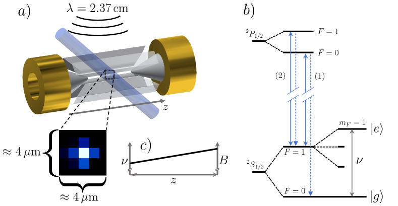
The spatial location of the ion is deduced from a measurement of the hyperfine resonance frequency, near 12.6 GHz corresponding to the magnetic dipole transition
in the elctronic ground state. Here, is the quantum number characterizing the total angular momentum and indicates the magnetic quantum number (Fig. 1).
The resonance frequency, is determined by the magnetic field at the location of the ion’s center of mass.
In order to implement RF-optical double-resonance spectroscopy [19], the ion is first Doppler cooled reaching a mean phonon number in the axial trapping potential. The ion is then initialized in state by applying laser radiation near 369 nm tuned to the resonance. Then, a single RF pulse of fixed duration and with variable frequency around the resonance of the transition is applied, generating a superposition state (). To measure the RF resonance frequency, the excitation probability of state has to be determined after the RF pulse is applied. This is achieved by applying a laser field near nm now resonant with the transition between states and . An ion in state scatters resonance fluorescence, an ion in state does not. The ion’s resonance fluorescence is collected and imaged onto an electron-multiplying charge coupled (EMCCD) camera. The ion’s internal state is projected on or depending on the outcome of this measurement [20]. This projective measurement is repeated typically 50 times to estimate .
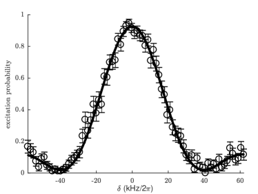
The excitation probability after an RF pulse with duration and frequency depends on the detuning from the resonance frequency. The duration of the RF pulse is chosen such that it corresponds to a pulse inverting the population of the states and when , that is, where is the Rabi frequency on resonance. An exemplary measurement of the hyperfine resonance is shown in Fig. 2. A fit of the experimental data allows for extracting the center frequency of the resonance line and thus the ion’s position in the magnetic gradient field.
A laser beam with beam waist of m is used to drive the optical resonance with a natural line width of MHz (Fig. 1). Imaging an ion’s resonance fluorescence onto the EMCCD camera allows for the reconstruction of the ion’s center-of-mass position with a spatial resolution of about nm [16, 17]. Here we demonstrate position measurements with a spatial resolution that is better by more than two orders of magnitude.
Lowering the Rabi frequency, by reducing the amplitude of the applied RF field, narrows down the resonance, thus enhancing the precision of determining and consequently of the position measurement.
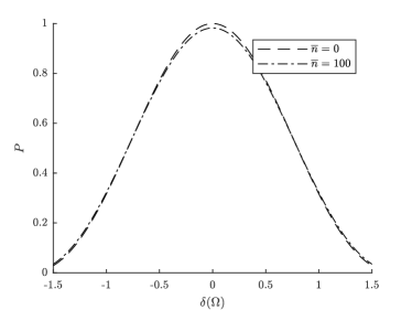
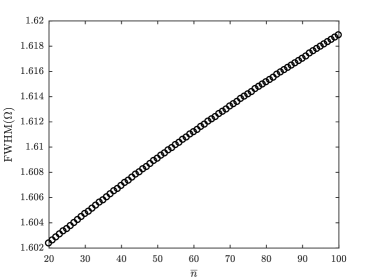
Excitation of the ion motion in the trapping potential will change the shape and width of the resonance, since the Rabi frequency depends on the ion’s vibrational excitation quantified by quantum number . This is taken account when fitting the resonance line in Fig. 2. Varying the mean phonon number of a thermal distribution in the range from 20 to 100 phonons yields a variation of the FWHM of the RF resonance by about 1 % making Doppler cooling sufficient for the precision of the position measurement desired in this work.
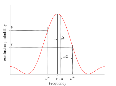
When tracking an ion’s position in real time, we determine its current resonance frequency from the measurement of the excitation probability for only two values of the detuning . Such a two-point frequency measurement reduces decisively the total measurement time required for determining the center frequency and is therefore more efficient as compared to the routinely employed technique of RF-optical double resonance spectroscopy [21] where the full resonance line is mapped out (Fig. 2).
These two measurements are carried out with the applied RF field symmetrically detuned such that . Here, is the estimated value for the current actual resonance frequency (except for the first measurement, is the result of the preceding determination of ). is chosen such as to separate the two measurement points by the FWHM of the hyperfine resonance as shown in Fig. 2.
We define to be the initially unknown offset of from the actual resonance frequency . The probabilities for detecting the ion in state when driving the resonance at frequency are . The function
| (1) |
maps the measured probabilities to the frequency offset , but is only injective as long as does not cross an extremal point of the resonance curve. Therefore, must fulfill . In this range, is monotonously increasing with . The calculation of therefore allows for extracting by searching for the closest match of the measured values of and . The standard deviation of determining (equal to the standard deviation of the ion’s resonance frequency) in the measurements reported here is (SM).
With a spatially constant magnetic field gradient [22], a shift in position can be deduced from a change in resonance frequency as
| (2) |
In the present setup, corresponds to a change in resonance frequency . Repeated measurements of the resonance frequency, employing the method described above, enable the experimenter to follow changes of an ion’s position by using the last measured frequency as a reference for the succeeding measurement.
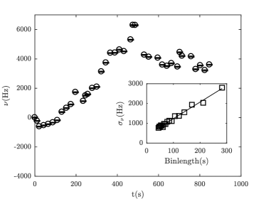
First, we measure the drift of an ion’s resonance frequency as a function of time (Fig. 4), without applying an additional static electric field that would deterministically shift the ion’s position. The observed drift could be caused by changes of an (uncontrolled) ambient electric field by shifting the ion’s position in the magnetic gradient field, and/or by an (uncontrolled) change of the ambient magnetic field at the ion’s position. The drift rate of Hz/s during this experiment is calculated using a fit to the Allan variance (Inset of Fig. 4) based on the measured frequencies shown in Fig. 4. The drift during the total time of 2 s needed to measure ion’s resonance frequency then amounts to Hz which translates into an uncertainty in determining the ion’s position of nm. This limits the spatial resolution of the current setup. Applying shielding for electric and magnetic fields [23], which is not present in the current experimental setup, will further increase the precision in determining an ion’s position.
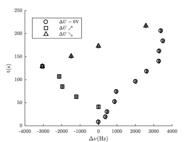
To demonstrate the capability of tracking an ion’s position, an imbalanced voltage, of varying magnitude is applied to the DC trapping electrodes shifting the ion’s equilibrium position along the z-axis (Fig. 1). Measurements of the ion’s resonance frequency, while applying V are alternated with measurements where V to correct the electric field-induced change in position for an unwanted drift. Fig. 5 shows the change of the ion’s resonance as a function of time. The measurements with in Fig. 5 indicate the unintended drift due to magnetic field drifts and possible voltage drifts during the experiment (the data points shown here are the same as in Fig. 4, corresponding to the time between s and s.) The change of the resonance frequency during the measurements with applied voltage, is interpolated between consecutive measurements with and subtracted from the absolute change in frequency. The resulting change in the ion’s position as a function of is shown in Fig. 5. In addition, Fig. 5 shows the change in the ion’s position calculated as a function of (dashed line) that matches well the measurements of the voltage-induced drift.
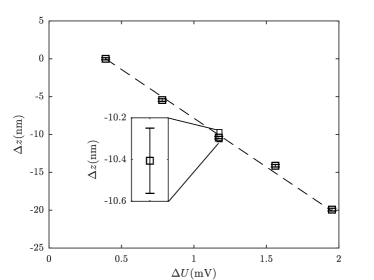
The standard deviation in determining the center of the resonance line in each measurement shown in Fig. 5 translates into a standard deviation of the ion’s position (SM, Eq. 1 and error propagation) as shown in Fig. 5. The mean standard deviation of all measurements of the ion’s position is 0.12 nm, and therefore yields a sub-wavelength resolution of .
From this position measurement, having characterized the trapping potential independently, a force displacing the ion can be derived. For the effective harmonic trapping potential used here, the constant of proportionality between displacement and force, is given by . This gives a force resolution of . Thus, for a measurement duration of 2 s we achieve a sensitivity of this static force measurement of . This force resolution would allow, for example, to detect a single elementary charge at a distance of .
Current limitations in the measurement time and the resolution of the position measurement can be overcome by continuous sympathetic cooling of the ion to be tracked by a second ion species. This will remove the necessity for Doppler cooling between measurements. Application of magnetic shielding will remove the necessity for maintaining a fixed phase relation of the measurement cycles with respect to the power line, thus further shortening the measurement time. A reduction of the uncontrolled ion drift by shielding against electric and magnetic fields will make it possible to carry out measurements at lower Rabi frequencies. We estimate that, using the method introduced here, the precision of position and force measurements could be enhanced further by several orders of magnitude (see SM).
We believe that the technique presented in this Letter can be adapted to other atomic and molecular ion systems with modest experimental effort. For example, this technique could be applied in the context of precision frequency metrology in order to detect, characterize and compensate for small shifts in the spatial position of single atomic [24] and molecular [25, 26, 27] ions. One may speculate about applying this technique to the detection of charges in particle physics. [28, 29].
While direct application of the demonstrated method in microscopy is beyond the capability of our current trap design, possible future devices can employ novel trap designs, for example a stylus trap [30], as a scanning probe with wavelength-relative spatial resolution orders of magnitude better than any state-of-the-art device known to us.
Acknowledgements.
The authors acknowledge funding from Deutsche Forschungsgemeinschaft and from the Bundesministerium für Bildung und Forschung (FK 16KIS0128). G. S. G. was supported by the European Commission’s Horizon 2020 research and innovation program under the Marie Skłodowska-Curie grant agreement number 657261.References
- Pohl et al. [1984] D. W. Pohl, W. Denk, and M. Lanz, Appl. Phys. Lett. 44, 651 (1984).
- Trautman et al. [1994] J. K. Trautman, J. J. Macklin, L. E. Brus, and E. Betzig, Nature 369, 40 (1994).
- Keilmann et al. [1996] F. Keilmann, D. van der Weide, T. Eickelkamp, R. Merz, and D. Stöckle, Opt. Commun. 129, 15 (1996).
- Kramer et al. [1996] A. Kramer, F. Keilmann, B. Knoll, and R. Guckenberger, Micron 27, 413 (1996).
- Zhang et al. [2017] H. Zhang, K. Arai, C. Belthangady, J.-C. Jaskula, and R. L. Walsworth, npj Quantum Information 3, 31 (2017).
- Jakobi et al. [2016] I. Jakobi, P. Neumann, Y. Wang, D. B. R. Dasari, F. E. Hallak, M. A. Bashir, M. Markham, A. Edmonds, D. Twitchen, and J. Wrachtrup, Nat. Nanotechnol. 12, 67 (2016).
- Sidles [1991] J. A. Sidles, Applied Physics Letters 58, 2854 (1991).
- Rugar et al. [1992] D. Rugar, C. S. Yannoni, and J. A. Sidles, Nature 360, 563 (1992).
- Degen et al. [2009] C. L. Degen, M. Poggio, H. J. Mamin, C. T. Rettner, and D. Rugar, Proceedings of the National Academy of Sciences 106, 1313 (2009).
- Kotler et al. [2011] S. Kotler, N. Akerman, Y. Glickman, A. Keselman, and R. Ozeri, Nature 473 (2011).
- Baumgart et al. [2016] I. Baumgart, J.-M. Cai, A. Retzker, M. B. Plenio, and C. Wunderlich, Phys. Rev. Lett. 116, 240801 (2016).
- Ruster et al. [2017] T. Ruster, H. Kaufmann, M. A. Luda, V. Kaushal, C. T. Schmiegelow, F. Schmidt-Kaler, and U. G. Poschinger, Phys. Rev. X 7, 031050 (2017).
- Knünz et al. [2010] S. Knünz, M. Herrmann, V. Batteiger, G. Saathoff, T. W. Hänsch, K. Vahala, and T. Udem, Phys. Rev. Lett. 105, 013004 (2010).
- Biercuk et al. [2010] M. J. Biercuk, H. Uys, J. W. Britton, A. P. VanDevender, and J. J. Bollinger, Nature Nanotechnology 5, 646 (2010).
- Maiwald et al. [2012] R. Maiwald, A. Golla, M. Fischer, M. Bader, S. Heugel, B. Chalopin, M. Sondermann, and G. Leuchs, Phys. Rev. A 86, 043431 (2012).
- Gloger et al. [2015] T. F. Gloger, P. Kaufmann, D. Kaufmann, M. T. Baig, T. Collath, M. Johanning, and C. Wunderlich, Phys. Rev. A 92, 043421 (2015).
- Blums et al. [2018] V. Blums, M. Piotrowski, M. I. Hussain, B. G. Norton, S. C. Connell, S. Gensemer, M. Lobino, and E. W. Streed, Science Advances 4, 10.1126/sciadv.aao4453 (2018).
- Khromova et al. [2012] A. Khromova, C. Piltz, B. Scharfenberger, T. F. Gloger, M. Johanning, A. F. Varón, and C. Wunderlich, Phys. Rev. Lett. 108, 220502 (2012).
- Brossel and Kastler [1949] J. Brossel and A. Kastler, Compt. Rend. 229, 1213 (1949).
- Wölk et al. [2015] S. Wölk, C. Piltz, T. Sriarunothai, and C. Wunderlich, Journal of Physics B: Atomic, Molecular and Optical Physics 48, 075101 (2015).
- Ludlow et al. [2015] A. D. Ludlow, M. M. Boyd, J. Ye, E. Peik, and P. O. Schmidt, Rev. Mod. Phys. 87, 637 (2015).
- Piltz et al. [2016] C. Piltz, T. Sriarunothai, S. S. Ivanov, S. Wölk, and C. Wunderlich, Sci. Adv. 2, e1600093 (2016).
- Ruster et al. [2016] T. Ruster, C. T. Schmiegelow, H. Kaufmann, C. Warschburger, F. Schmidt-Kaler, and U. G. Poschinger, Applied Physics B 122, 254 (2016).
- Schmidt et al. [2005] P. O. Schmidt, T. Rosenband, C. Langer, W. M. Itano, J. C. Bergquist, and D. J. Wineland, Science 309, 749 (2005).
- Wolf et al. [2016] F. Wolf, Y. Wan, J. C. Heip, F. Gebert, C. Shi, and P. O. Schmidt, Nature 530, 457 (2016).
- wen Chou et al. [2017] C. wen Chou, C. Kurz, D. B. Hume, P. N. Plessow, D. R. Leibrandt, and D. Leibfried, Nature 545, 203 (2017).
- Sinhal et al. [2020] M. Sinhal, Z. Meir, K. Najafian, G. Hegi, and S. Willitsch, Science 367, 1213 (2020).
- Carney et al. [2021] D. Carney, H. Häffner, D. C. Moore, and J. M. Taylor, Phys. Rev. Lett. 127, 061804 (2021).
- Budker et al. [2021] D. Budker, P. W. Graham, H. Ramani, F. Schmidt-Kaler, C. Smorra, and S. Ulmer, Millicharged dark matter detection with ion traps (2021), arXiv:2108.05283 .
- Maiwald et al. [2009] R. Maiwald, D. Leibfried, J. Britton, J. C. Bergquist, G. Leuchs, and D. J. Wineland, Nature Physics 5, 551 (2009).