Overlapping substitutions and tilings

Abstract.

Inspired by [17], we generalize the notion of (geometric) substitution rule to obtain overlapping substitutions. For such a substitution, the substitution matrix may have non-integer entries. We give the meaning of such a matrix by showing that the right Perron–Frobenius eigenvector gives the patch frequency of the resulting tiling. We also show that the expansion constant is an algebraic integer under mild conditions. In general, overlapping substitutions may yield a patch with contradictory overlaps of tiles, even if it is locally consistent. We give a sufficient condition for an overlapping substitution to be consistent, that is, no such contradiction will emerge. We also give many one-dimensional examples of overlapping substitution. We finish by mentioning a construction of overlapping substitutions from Delone multi-sets with inflation symmetry.

1. Introduction

Given a finite set of symbols ${\mathcal{A}}$, we denote by ${\mathcal{A}}^{*}$ the semi-group generated by concatenation of letters in ${\mathcal{A}}$ equipped with an empty word $\lambda$ as an identity. A substitution $\sigma$ is a rule to replace each letter by a word in ${\mathcal{A}}^{+}={\mathcal{A}}\setminus\{\lambda\}$, which naturally extends to a morphism on ${\mathcal{A}}^{*}$ by homeomorphy $\sigma(xy)=\sigma(x)\sigma(y)$ for $x,y\in{\mathcal{A}}^{*}$. Substitutions give a tool and a toy model to describe the self-inducing structure of dynamical systems. For $w\in{\mathcal{A}}^{*}$ and $i\in{\mathcal{A}}$, let $|w|_{i}$ be the number of letter $i$ in $w$. The substitution matrix $M_{\sigma}=(|\sigma(j)|_{i})$ gives a basic statistical information of $\sigma$. A substitution $\sigma$ is called primitive if $M_{\sigma}$ is primitive, i.e., there exists a positive integer $n$ such that $(M_{\sigma})^{n}$ is a positive matrix. By Perron–Frobenius theory, if $\sigma$ is primitive, then there exists a unique positive dominant eigenvalue $\beta$ of $M_{\sigma}$, called Perron–Frobenius root, which represents the growth rate of the associated dynamical system (c.f.[2, Chapter 4]). Given a primitive substitution $\sigma$, and fix a left eigenvector $(\ell_{1},\dots,\ell_{\kappa})$ corresponds to the Perron–Frobenius root $\beta$. Then the substitution has a nice geometric realization into a $1$-dimensional self-similar tiling. Each tile is the interval $A_{i}=[0,\ell_{i}]\ (i=1,\dots,{\kappa})$. Then we obtain

(1.1) $$\beta A_{j}=\bigcup_{i=1}^{\kappa}(A_{i}+D_{ij})=\bigcup_{i=1}^{\kappa}\bigcup_{d\in D_{ij}}(A_{i}+d)$$

where $D_{ij}$ is a finite set of translation vectors in ${\mathbb{R}}$ with $M_{\sigma}=(\text{Card}(D_{ij}))_{1\leq i,j\leq{\kappa}}$ and the union appears in the right side are disjoint in measure, i,e., two tiles do not share an inner point. Iterating this process indefinitely, we obtain a tiling of ${\mathbb{R}}$ by the intervals $A_{i}$ and their translations.

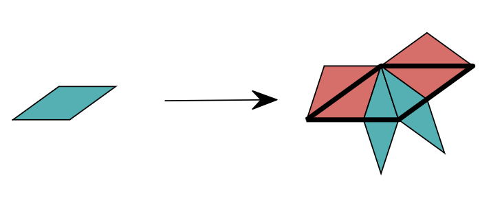
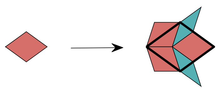
Figure 1. Penrose tiling substitution

Figure 2. Ammann-Beenker tiling substitution

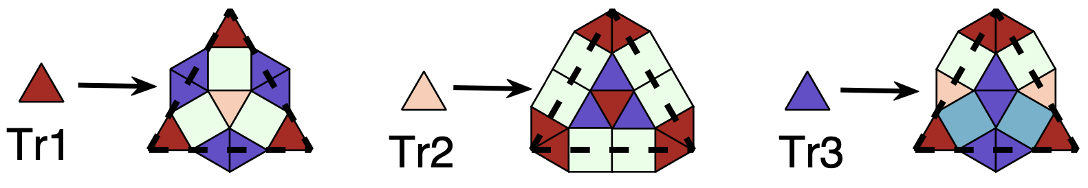
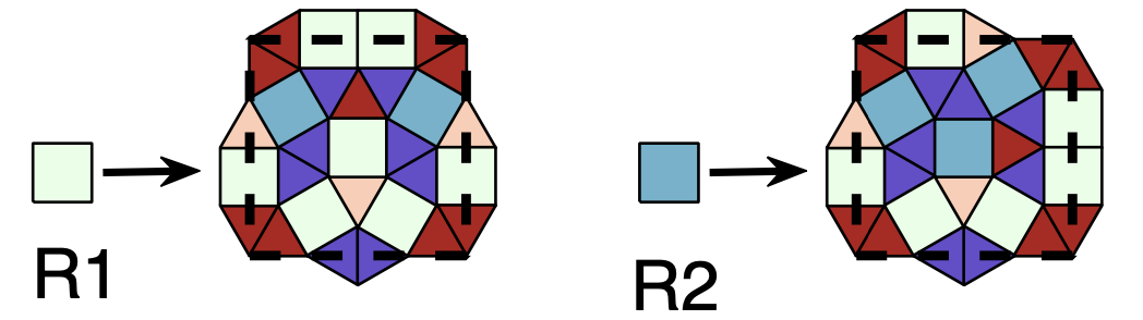
Figure 3. Square Triangle tiling substitution

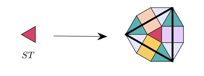
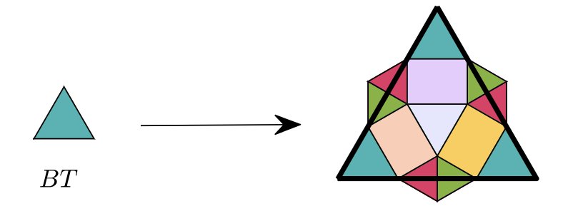
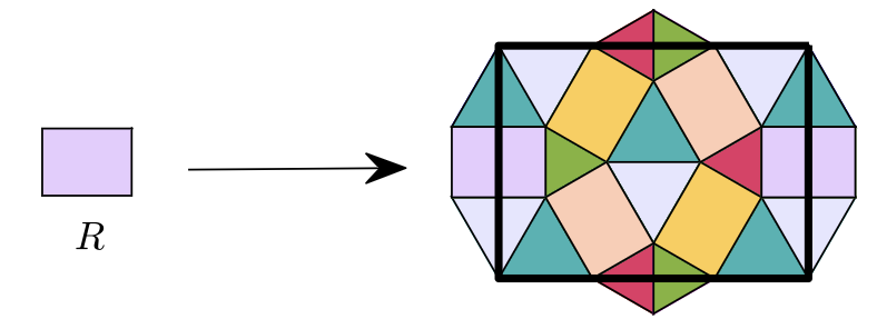
Figure 4. Bronze-mean tiling substitution

Self-similar tiling in ${\mathbb{R}}^{d}$ is a natural generalization of this construction (c.f. [15]). Given non-empty compact sets $A_{i}\ (i=1,\dots,{\kappa})$ which coincide with the closure of its interior, i.e., $A_{i}=\overline{A_{i}^{\circ}}$. We assume that they satisfy the same equation (1.1) in ${\mathbb{R}}^{d}$ and assume that the union is disjoint in measure. If $(\text{Card}(D_{ij}))$ is primitive, then successive inflation $\times\beta$ of each tile and subdivision to the corresponding tiles, we get larger and larger patches. Assuming finite local complexity of patches, that is, finiteness of local configurations up to translation, we obtain a tiling of ${\mathbb{R}}^{d}$ by $A_{i}\ (i=1,\dots,{\kappa})$ and its translations by standard argument. Every patch is a sub-patch of some inflation of a single tile $A_{1}$, say. By endowing labels to tiles if necessary, many historical non-periodic tilings fall into this flame work and serve as a nice model of self-inducing structure and quasi-crystals, the real matter that possesses long-range order with no translational period.

In this article, we wish to study a generalization of the concept, by allowing the overlap of pieces, in the sense that the tile does not exactly satisfy the equation like (1.1). In fact, the polygonal substitutions of Penrose tiling (see Figure 1) and that of Ammann-Beenker tiling (see Figure 2) had the same problem, but they are finally reduced to the tiles satisfying (1.1) by suitable sub-tiles or considering its limit shapes which usually have fractal boundaries.

Our motivating examples are the substitution depicted in Figures 3 and 4. Figure 3 is found by Schlottman, whose descriptions are studied in [2] and [7]. It is not known to be mutually locally derivable from a tiling satisfying (1.1). Therefore the situation around this tiling is not crystalline clear yet. The substitution in Figure 4 was introduced by Dotera-Bekku-Ziher [17]. The expanded tiles are expressed by bold lines in the figure. We can iterate this substitution seemingly without problem. Identifying rotated tiles, the figure suggests its associated substitution matrix

$$\begin{pmatrix}1&3&4\\ 3&4&8\\ 3/2&3&5\end{pmatrix}$$

contains, astonishingly, a non-integer entry $3/2$. Here the 1-st column means the inflation of ST tile by bronze mean contains 1 ST tile, 3 BT tiles and 3/2 R tiles, as we count the tiles within the bold line triangle in Figure 4. It is seemingly “irrational” and we see no easy way to reduce it to the usual substitution setting. Moreover, there is no justification for whether this substitution could be indefinitely iterated without partial overlaps of tiles, i.e., it is globally well-defined. We notice that the same question in Figure 3 exists as well.

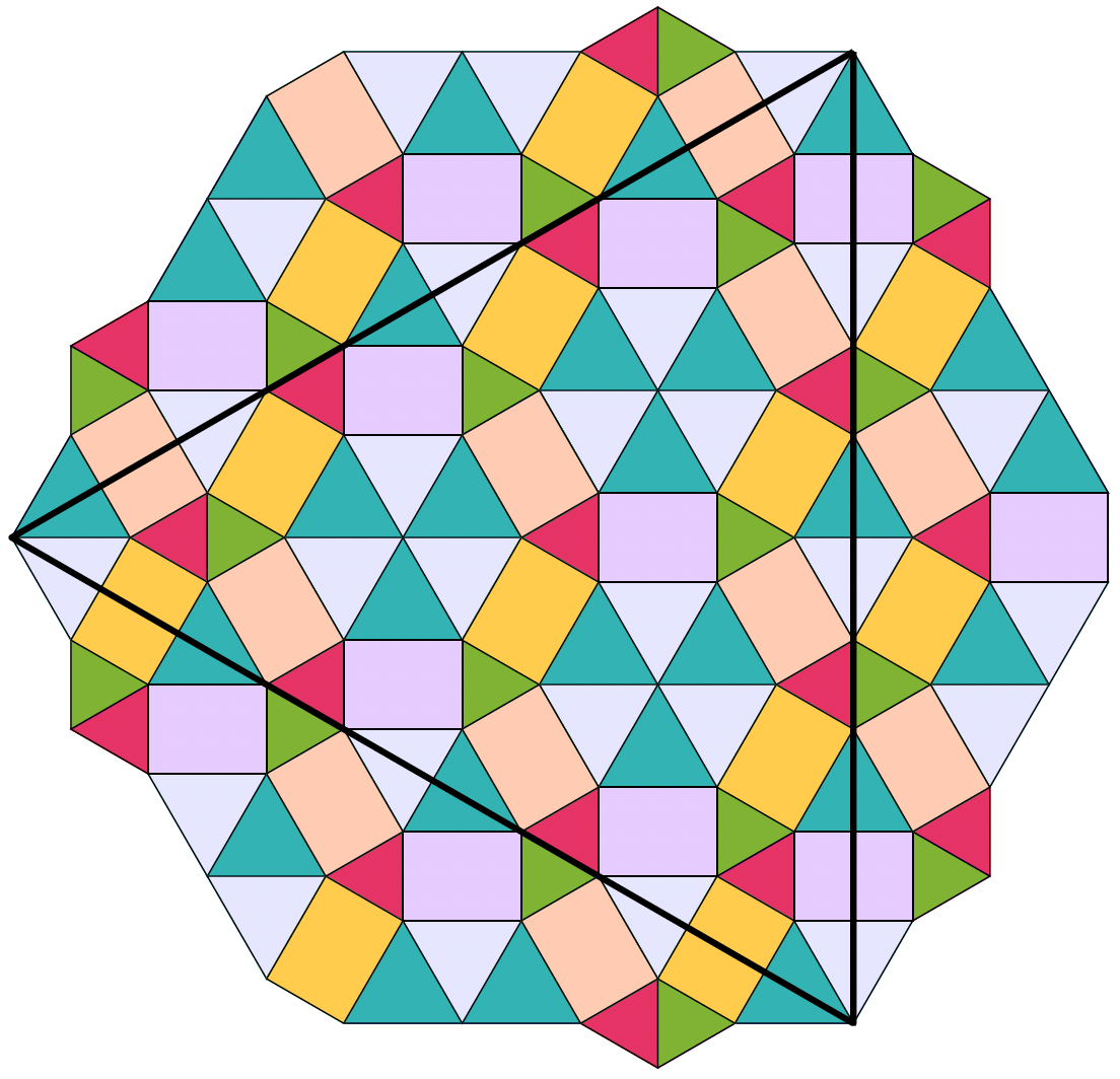
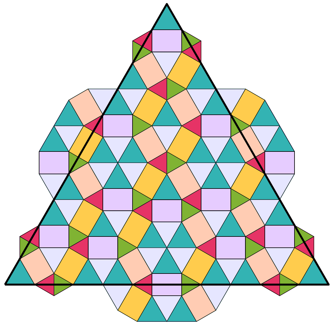
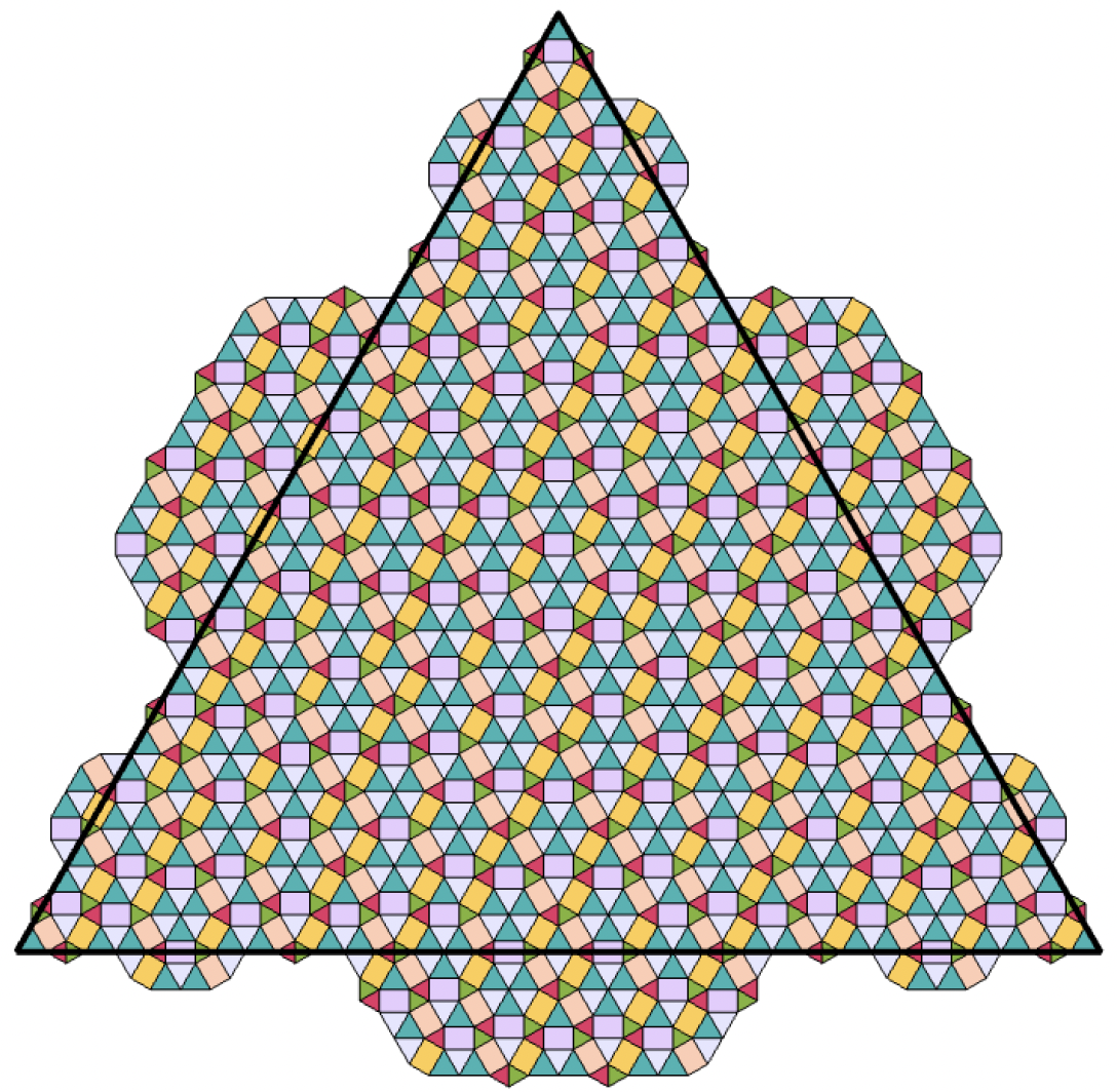
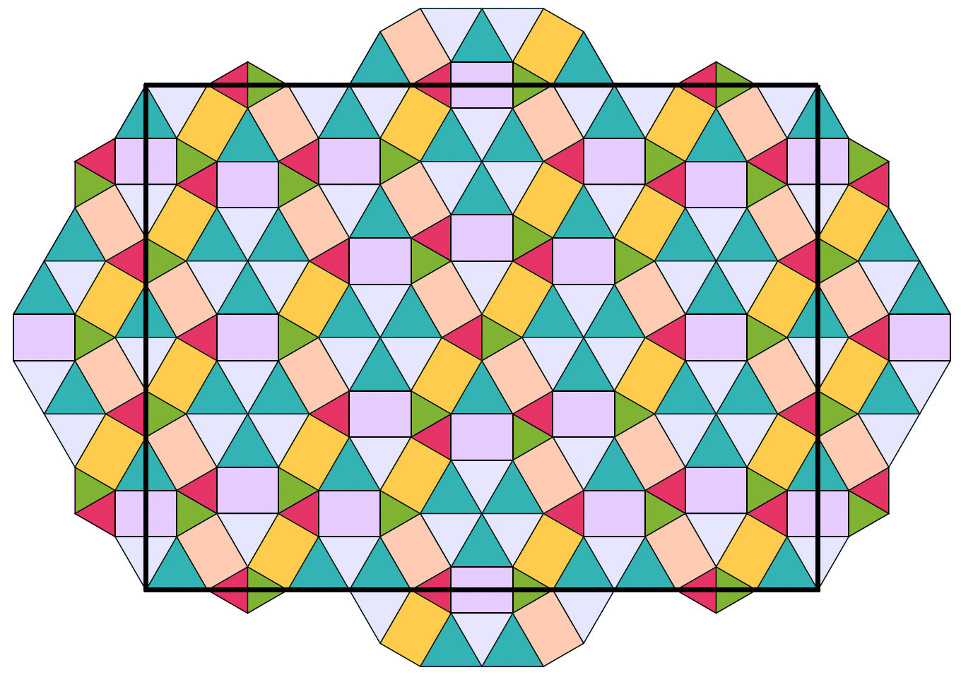
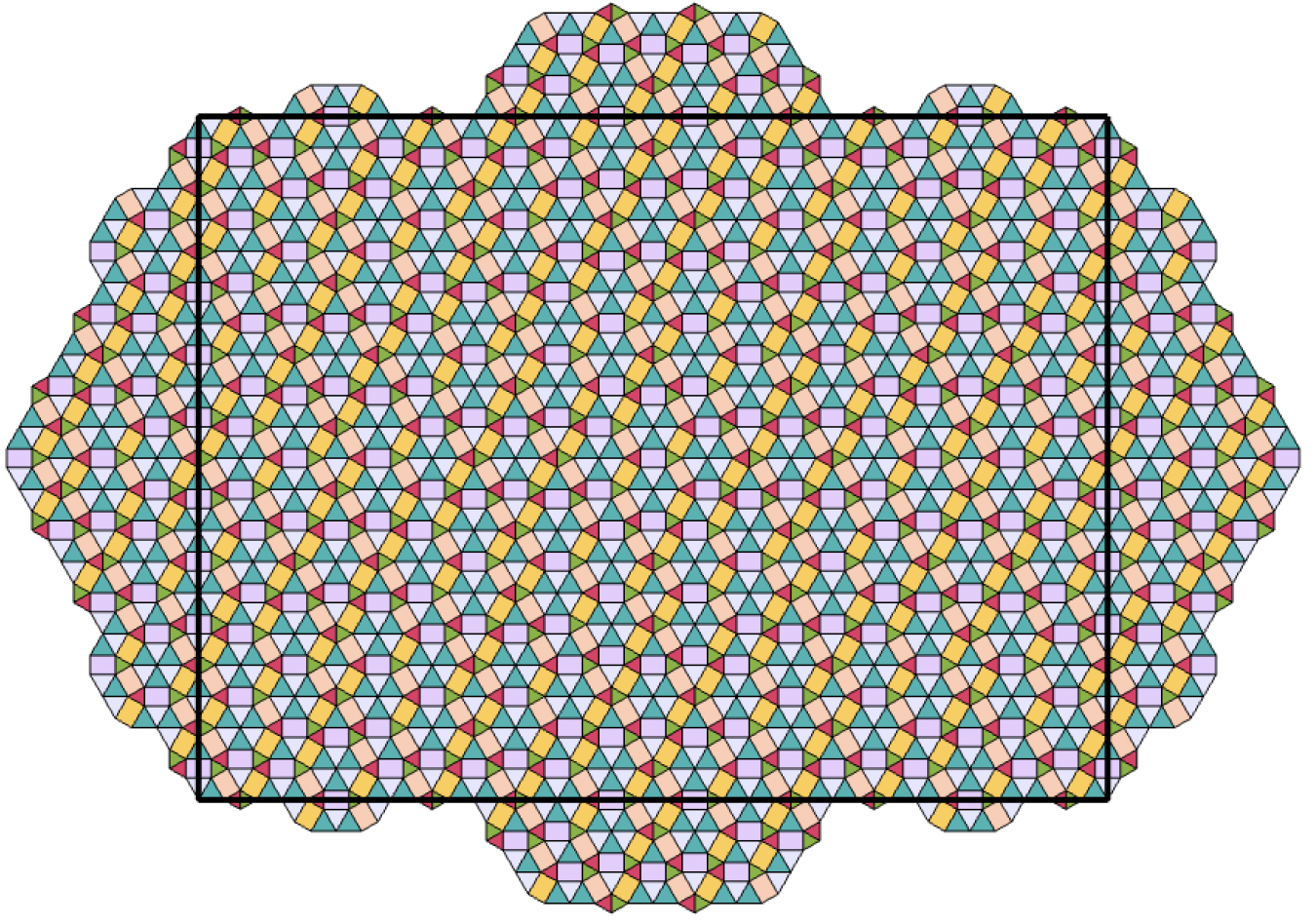
Figure 5. The second and third iteration of Bronze-means ’tiles’ starting with ‘ST’, ‘BT’ and ‘R’.

There exists another motivating example in one dimension.

Example 1.1 (One dimensional overlapping substitution).

Let $\sigma$ be a substitution over $\{a,b,c\}$ as follows.

$$\sigma:\left\{\begin{aligned} a&\longrightarrow\frac{a}{2}ba\\ b&\longrightarrow c\frac{a}{2}\\ c&\longrightarrow b\frac{a}{2}\end{aligned}\right.$$

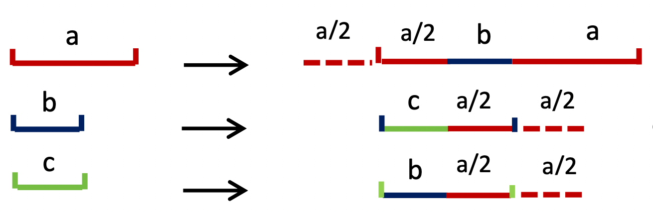
Figure 6. Substitution of Example 1.1

The notation $a/2$ is understood similarly as in Figure 4, telling us that half of the tile $a$ is outside of the enlarged original tile (see dotted line in Figure 6). The substitution matrix of this $\sigma$ is

$$\begin{pmatrix}3/2&1/2&1/2\\ 1&0&1\\ 0&1&0\end{pmatrix},$$

having non-integer entries again. We can iterate this substitution naturally because the overlapping symbols match without causing problems. For example, if we start from a patch $ba$

$$\sigma(ba)=c\frac{a}{2}\frac{a}{2}ba=caba$$

$$\sigma^{2}(ba)=b\frac{a}{2}\frac{a}{2}bac\frac{a}{2}\frac{a}{2}ba=babacaba$$

$$\sigma^{3}(ba)=c\frac{a}{2}\frac{a}{2}bac\frac{a}{2}\frac{a}{2}bab\frac{a}{2}\frac{a}{2}bac\frac{a}{2}\frac{a}{2}ba=cabacabababacaba$$

Here we consider concatenating two $\frac{a}{2}$ by $a$.

We think it is a good time to initiate a systematic study of such “overlapping” substitutions with mathematical rigor and to deliver answers to the above questions. This article is the first attempt to give possible definitions of overlapping substitution and explore their basic properties.

The rest of the paper is organized as follows. As we introduce the overlap of tiles, the most suitable way to describe the tile substitution is found in the function setting. Therefore in Section 2 we give the basic theory of weighted substitutions and the definition of overlapping substitutions. Our goal is to apply the Perron–Frobenius theory to an appropriate function space and apply it to our tilings. In Section 3, we show that the expansion constant of the overlapping substitution must be an algebraic integer under mild conditions. In Section 4, we discuss the global consistency problem of the two-dimensional overlapping substitutions. We show that the known overlapping substitutions are well-defined using fractal geometry. In Section 5, we construct overlapping substitution in one dimension. We find several parametric families of overlapping substitutions whose tile sizes vary according to the parameters. Finally, we construct overlapping substitutions from Delone set with inflation symmetry, in arbitrary dimension.

2. The theory of weighted substitutions and overlapping substitutions

2.1. Definitions of tiles, patches and tilings

Let $L$ be a finite set. An $L$-labeled tile is a pair $T=(S,l)$ where $l\in L$, $S\subset\mathbb{R}^{d}$ is compact non-empty and $S=\overline{S^{\circ}}$, that is, the closure of the interior of $S$ coincides with $S$. If we do not specify the set $L$ of labels, the $L$-labeled tiles are just called labeled tiles. There are also unlabeled tiles, that are by definition a compact and non-empty $S\subset\mathbb{R}^{d}$ such that $S=\overline{S^{\circ}}$. Both labeled tiles and unlabeled tiles are called tiles. For a labeled tile $T=(S,l)$, we use a notation $\operatorname{supp}T=S$ and $\operatorname{int}T=S^{\circ}$. We define the translate of $T$ by $x\in\mathbb{R}^{d}$ via $T+x=(S+x,l)$. For an unlabeled tile $S$, we use a notation $\operatorname{supp}S=S$ and $\operatorname{int}S=S^{\circ}$. We give a presentation that deals with both labeled and unlabeled tiles by these notations.

A set consisting of tiles is called a pattern. A pattern $\mathcal{P}$ such that $S,T\in\mathcal{P}$ and $\operatorname{int}S\cap\operatorname{int}T\neq\emptyset$ imply $S=T$ is called a patch. We say two tiles $S,T$ in a pattern are an illegal overlap if $S\neq T$ and $\operatorname{int}S\cap\operatorname{int}T\neq\emptyset$. A patch is a pattern without any illegal overlaps. For a patch $\mathcal{T}$, we define its support $\operatorname{supp}\mathcal{T}$ via

$$\operatorname{supp}\mathcal{T}=\bigcup_{T\in\mathcal{T}}\operatorname{supp}T.$$

A patch $\mathcal{T}$ such that $\operatorname{supp}\mathcal{T}=\mathbb{R}^{d}$ is called a tiling. A translate of a pattern $\mathcal{P}$ by a vector $x\in\mathbb{R}^{d}$ is defined via

$$\mathcal{P}+x=\{T+x\mid T\in\mathcal{P}\}.$$

2.2. The theory of weighted substitutions

Let $\mathcal{B}$ be a finite set of tiles. We use notation $\mathcal{B}+\mathbb{R}^{d}$ for the set of all the translates of the tiles in $\mathcal{B}$, that is, the set of all tiles $T+x$ where $T\in\mathcal{B}$ and $x\in\mathbb{R}^{d}$. In this section, we consider weights on the tiles in patches. For example, we start with two patches $\mathcal{P}_{1}=\{[0,1],[1,2]\}$ and $\mathcal{P}_{2}=\{[1,2],[2,3]\}$ whose elements are intervals, and we consider weights on each tile, for example

1. the weight of $[0,1]$ in $\mathcal{P}_{1}$ is $2/3$ and one of $[1,2]$ in $\mathcal{P}_{1}$ is $3/4$, and

2. the weight of $[1,2]$ in $\mathcal{P}_{2}$ is $1/2$ and one of $[2,3]$ in $\mathcal{P}_{2}$ is $1$.

(The choice of numbers can be arbitrary.) Without weights, the union $\mathcal{P}_{1}\cup\mathcal{P}_{2}$ is $\{[0,1],[1,2],[2,3]\}$, but with weights, if we take the union, the weights of the overlapping tiles add up, and so the result is a patch $\{[0,1],[1,2],[2,3]\}$ with a weight $2/3$ on $[0,1]$, $5/4$ on $[1,2]$ and $1$ on $[2,3]$. The readers may notice that this is exactly what functions on patches are. However, we do not deal with functions $v_{1}\colon\mathcal{P}_{1}\rightarrow\mathbb{R}$ and $v_{2}\colon\mathcal{P}_{2}\rightarrow\mathbb{R}$, because these cannot be added since the domains are different. Instead, we should consider maps $v_{1}$ and $v_{2}$ to which we can plug in arbitrary tiles in $\mathbb{R}$. The values for $v_{1}$ should be

$$v_{1}(T)=\begin{cases}2/3&\text{if $T=[0,1]$}\\ 3/4&\text{if $T=[1,2]$}\\ 0&\text{otherwise.}\end{cases}$$

We endow values for $v_{2}$ in an appropriate way. In what follows, we study such functions on $v\colon\mathcal{B}+\mathbb{R}^{d}\rightarrow\mathbb{R}$, where $\mathcal{B}$ is a given finite set of tiles.

Let us enumerate the tile in $\mathcal{B}$ so that we have $\mathcal{B}=\{T_{1},T_{2},\ldots T_{\kappa}\}$. A map $v\colon\mathcal{B}+\mathbb{R}^{d}\rightarrow\mathbb{R}$ is called a weighted pattern with alphabet $\mathcal{B}$. The set of all weighted patterns with alphabet $\mathcal{B}$ is denoted by $\mathcal{W}\mathcal{P}_{\mathcal{B}}$. This is a vector space over $\mathbb{R}$.

On $\mathcal{W}\mathcal{P}_{\mathcal{B}}$, we define the weak topology. Consider all the maps

$$\tau_{T}\colon\mathcal{W}\mathcal{P}_{\mathcal{B}}\ni v\mapsto v(T)\in\mathbb{R},$$

where $T$’s are arbitrary elements of $\mathcal{B}+\mathbb{R}^{d}$. The weak topology is the weakest topology which makes all these maps continuous.

For a weighted pattern $v$ with alphabet $\mathcal{B}$, its support pattern is

$$\operatorname{SP}(v)=\{T\in\mathcal{B}+\mathbb{R}^{d}\mid v(T)\neq 0\}$$

Its support region is

$$\operatorname{SR}(v)=\overline{\bigcup_{v(T)\neq 0}\operatorname{supp}T}.$$

Next, we define a weighted substitution. Consider a linear and expanding map $\phi\colon\mathbb{R}^{d}\rightarrow\mathbb{R}^{d}$. Consider also a map $\xi\colon\mathcal{B}\rightarrow\mathcal{W}\mathcal{P}_{\mathcal{B}}$ such that, for each $T\in\mathcal{B}$,

1. $\operatorname{SP}(\xi(T))$ is a finite set, and

2. $\xi(T)$ is a positive map, that is, for any $S\in\mathcal{B}+\mathbb{R}^{d}$, we have $\xi(T)(S)\geqq 0$.

We call the triple $(\mathcal{B},\phi,\xi)$ a pre-weighted substitution, or we just simply say $\xi$ a pre-weighted substitution with alphabet $\mathcal{B}$. At this stage we do not assume any relations between $\xi$ and $\phi$. In what follows, we will define iterates of $\xi$, and we call $\xi$ a weighted substitution if, after applying arbitrary iterates of $\xi$ to any tile $T\in\mathcal{B}$, the support pattern is a patch, that is, no partial overlaps (Definition 1).

We extend the domain of pre-weighted substitution as for the usual substitution rules. For $T\in\mathcal{B}$ and $x\in\mathbb{R}^{d}$, set

$$\xi(T+x)(S)=\xi(T)(S-\phi(x)),$$

where $S$ is an arbitrary element of $\mathcal{B}+\mathbb{R}^{d}$. In this way, we obtain a map

$$\xi\colon\mathcal{B}+\mathbb{R}^{d}\rightarrow\mathcal{W}\mathcal{P}_{\mathcal{B}}.$$

It is easy to prove that

$$\operatorname{SP}(\xi(T+x))=\operatorname{SP}(\xi(T))+\phi(x).$$

Given a weighted substitution $\xi$, we define a substitution matrix for it. For a $v\in\mathcal{W}\mathcal{P}_{\mathcal{B}}$ with finite $\operatorname{SP}(v)$ and $T\in\mathcal{B}$, we set

$$\tau_{T}(v)=\sum_{x\in\mathbb{R}^{d}}v(T+x).$$

Note that the sum is finite, i.e., there are only finitely many positive terms. The substitution matrix for $\xi$ is the $\kappa\times\kappa$ matrix whose $(i,j)$ element is $\tau_{T_{i}}(\xi(T_{j}))$. A weighted substitution $\xi$ is said to be primitive if its substitution matrix is primitive.

Next, we will further “extend” the domain for $\xi$ to $\mathcal{W}\mathcal{P}_{\mathcal{B}}$.

Lemma 2.1.

For any $T\in\mathcal{B}+\mathbb{R}^{d}$, there are only finitely many $S\in\mathcal{B}+\mathbb{R}^{d}$ such that $\xi(S)(T)\neq 0$.

Proof.

If $S\in\mathcal{B}+\mathbb{R}^{d}$ and $\xi(S)(T)\neq 0$, there are $P\in\mathcal{B}$ and $x\in\mathbb{R}^{d}$ such that $S=P+x$, and $\xi(P)(T-\phi(x))\neq 0$. We have an injection

$$\{S\mid\xi(S)(T)\neq 0\}\ni S\mapsto(P,T-\phi(x))\in\{(P,U)\mid P\in\mathcal{B},U\in\operatorname{SP}(\xi(P))\}.$$

∎

Lemma 2.2.

For any $v\in\mathcal{W}\mathcal{P}_{\mathcal{B}}$, the sum

$$\sum_{T\in\operatorname{SP}(v)}v(T)\xi(T)$$

is convergent with respect to the weak topology, that is, for any $S\in\mathcal{B}+\mathbb{R}^{d}$, there is a real number $\alpha$ such that, for any $\varepsilon>0$, there is a finite set $F\subset\operatorname{SP}(v)$ with

$$\left|\sum_{T\in F^{\prime}}v(T)\xi(T)(S)-\alpha\right|<\varepsilon$$

for any finite $F^{\prime}$ with $F\subset F^{\prime}\subset\operatorname{SP}(v)$.

Proof.

For each $S\in\mathcal{B}+\mathbb{R}^{d}$, by Lemma 2.1, the set

$$\{T\in\operatorname{SP}(v)\mid\xi(T)(S)\neq 0\}$$

is finite, and so

$$\sum_{T\in\operatorname{SP}(v)}v(T)\xi(T)(S)$$

is a finite sum. ∎

We set

$$\xi(v)=\sum_{T\in\operatorname{SP}(v)}v(T)\xi(T)=\sum_{T\in\mathcal{B}+\mathbb{R}^{d}}v(T)\xi(T),$$

and so we have a map

$$\xi\colon\mathcal{W}\mathcal{P}_{\mathcal{B}}\rightarrow\mathcal{W}\mathcal{P}_{\mathcal{B}}.$$

Definition 1.

The pre-weighted substitution is said to be consistent if the support pattern for $\xi^{n}(\delta_{T})$ is a patch (that is, no illegal overlaps) for any $n>0$ and $T\in\mathcal{B}$, where $\delta_{T}$ is defined via

$$\delta_{T}(S)=\begin{cases}1&\text{ if $T=S$}\\ 0&\text{ otherwise.}\end{cases}$$

Lemma 2.3.

The map

$$\xi\colon\mathcal{W}\mathcal{P}_{\mathcal{B}}\ni v\mapsto\xi(v)\in\mathcal{W}\mathcal{P}_{\mathcal{B}}$$

is linear and continuous with respect to the weak topology.

Proof.

That the map is linear is easy to be proved. To prove the continuity, take an arbitrary $S\in\mathcal{B}+\mathbb{R}^{d}$. By Lemma 2.1, the set

$$\mathcal{F}=\{T\in\mathcal{B}+\mathbb{R}^{d}\mid\xi(T)(S)\neq 0\}$$

is a finite set. If $v,v^{\prime}\in\mathcal{W}\mathcal{P}_{\mathcal{B}}$ are close enough in the sense that

$$v(T)\approx v^{\prime}(T)$$

for any $T\in\mathcal{F}$, then

$$\sum_{T\in\mathcal{B}+\mathbb{R}^{d}}v(T)\xi(T)(S)\approx\sum_{T\in\mathcal{B}+\mathbb{R}^{d}}v^{\prime}(T)\xi(T)(S)$$

and so $\xi(v)(S)\approx\xi(v^{\prime})(S)$. ∎

Corollary 2.4.

$$\xi^{n}(v)=\sum_{T\in\mathcal{B}+\mathbb{R}^{d}}v(T)\xi^{n}(T).$$

For the usual theory for tilings, the cutting-off operation is important. We define the cutting-off operation for weighted patches. For a $v\in\mathcal{W}\mathcal{P}_{\mathcal{B}}$ and a $K\subset\mathbb{R}^{d}$ we define the cut-off $v\wedge K$ of $v$ by $K$ via

$$v\wedge K(T)=\begin{cases}v(T)&\text{ if $\operatorname{supp}T\subset K$}\\ 0&\text{ otherwise.}\end{cases}$$

Lemma 2.5.

For any $K\subset\mathbb{R}^{d}$, the map

$$\mathcal{W}\mathcal{P}_{\mathcal{B}}\ni v\mapsto v\wedge K\in\mathcal{W}\mathcal{P}_{\mathcal{B}}$$

is linear and continuous with respect to the weak topology.

Proof.

Take a $T\in\mathcal{B}+\mathbb{R}^{d}$ and fix it. If $\operatorname{supp}T\not\subset K$ then $v\wedge K(T)=0$ for any $v$. Otherwise, if $v(T)\approx v^{\prime}(T)$, then $v\wedge K(T)=v(T)\approx v^{\prime}(T)=v^{\prime}\wedge K(T)$. ∎

Finally in this section, we prove that the right Perron–Frobenius eigenvector gives the frequency for the fixed point for $\xi$.

Proposition 2.6.

Let $v$ be such that

1. $\operatorname{SP}(v)$ is a tiling in $\mathbb{R}^{d}$,

2. $v(T)=1$ for any $T\in\operatorname{SP}(v)$,

3. $\xi^{k}(v)=v$ for some $k>0$, and

4. the substitution matrix for $v$ is primitive.

Take a left Perron–Frobenius left eigenvector $l=(l_{1},l_{2},\ldots,l_{\kappa})$ and right eigenvector

$$r=\begin{pmatrix}r_{1}\\ r_{2}\\ \vdots\\ r_{\kappa}\end{pmatrix}$$

for the substitution matrix for $\xi$, and assume $l_{i}$ coincides with the Lebesgue measure $\operatorname{vol}(\operatorname{supp}T_{i})$ for $\operatorname{supp}T_{i}$ for each $i$, and $l$ and $r$ are normalized in the sense that $\sum_{i=1}^{\kappa}l_{i}r_{i}=1$.

Then $r$ describes the frequency for $v$, which is regarded as a tiling: for any van Hove sequence $(A_{n})_{n=1,2,\ldots}$ and $x_{1},x_{2},\ldots\in\mathbb{R}^{d}$, we have a convergence

$$\lim_{n\rightarrow\infty}\frac{1}{\operatorname{vol}(A_{n})}\tau_{T_{i}}(v\wedge(A_{n}+x_{n}))=r_{i},$$

which is uniform for $(x_{n})$.

The proof will be given in the appendix.

2.3. The theory of overlapping substitutions

A pre-overlapping substitution is a triple $(\mathcal{B},\phi,\rho)$ where

• $\mathcal{B}=\{T_{1},T_{2},\ldots,T_{\kappa}\}$ is a finite set of tiles in $\mathbb{R}^{d}$,

• $\phi\colon\mathbb{R}^{d}\rightarrow\mathbb{R}^{d}$ is a linear map of which eigenvalues are all greater than 1 in modulus, and

• $\rho$ is a map defined on $\mathcal{B}$ such that $\rho(T_{i})$ is a finite patch consisting of translates of elements of $\mathcal{B}$.

The set $\mathcal{B}$ is called the alphabet for the pre-overlapping substitution and each $T_{i}$ in $\mathcal{B}$ is called a proto-tile. For a proto-tile $T_{i}$ and $x\in\mathbb{R}^{d}$, we set

$$\rho(T_{i}+x)=\rho(T_{i})+\phi(x).$$

For a pattern $\mathcal{P}$ consisting of translates of proto-tiles, we set

$$\rho(\mathcal{P})=\bigcup_{T\in\mathcal{P}}\rho(T).$$

Note that each $\rho(T)$ is already defined and $\rho(\mathcal{P})$ is a new pattern consisting of translates of proto-tiles. We use the same symbol $\rho$ for an pre-overlapping substitution and a map that sends a pattern to another pattern. For a pattern $\mathcal{P}$ consisting of translates of proto-tiles, we can apply $\rho$ multiple times and obtain $\rho^{n}(\mathcal{P})$ for $n=1,2,\ldots$. If, for any $n>0$ and proto-tile $T$, the pattern $\rho^{n}(T)$ is a patch (no illegal overlaps), then we say $\rho$ is consistent and call $\rho$ an overlapping substitution.

To an overlapping substitution $\rho$, we can often take a patch $\mathcal{P}$ consisting of translates of proto-tiles such that for each $n=1,2,\ldots$, the set $\rho^{n}(\mathcal{P})$ is a patch, that is, no illegal overlaps. Moreover, we often have that, for some $k>0$,

$$\lim_{n\rightarrow\infty}\rho^{kn}(\mathcal{P})$$

converges to a tiling and so we have a fixed point for an overlapping substitution $\rho^{k}$.

For an expanging overlapping substitution, the above process is almost always possible, given a primitivity condition is satisfied. We say an overlapping substitution $(\mathcal{B},\phi,\rho)$ is expanding if for each $P\in\mathcal{B}$, we have

$$\operatorname{supp}\rho(P)\supset\phi(\operatorname{supp}P).$$

For an expanding overlapping substitution $\rho$, if we can find a $P\in\mathcal{B}$ and an $x\in\mathbb{R}^{d}$ such that

$$P+x\in\rho^{k}(P+x),$$

and $P+x$ is in the “interior” of the right-hand side, then by an standard argument, we can construct a tiling

$$\mathcal{T}=\lim_{n\rightarrow\infty}\rho^{kn}(P+x),$$

which is a fixed point for $\rho$: we have $\rho^{k}(\mathcal{T})=\mathcal{T}$.

To an overlapping substitution $(\mathcal{B},\phi,\rho)$, we can associate a weighted substitution $(\mathcal{B},\phi,\tilde{\rho})$, as follows. The alphabet and the expansion map are the same. For $T_{i}\in\mathcal{A}$, the weighted patch $\tilde{\rho}(T_{i})$ is a map whose support is $\rho(T_{i})$ and the weights are defined via

$$\tilde{\rho}(T_{i})(S)=\frac{\operatorname{vol}(\phi(\operatorname{supp}T_{i})\cap\operatorname{supp}S)}{\operatorname{vol}(\operatorname{supp}S)},$$

where $\operatorname{vol}$ denotes the Lebesgue measure and $S\in\rho(T_{i})$. Note that this computation of substitution matrix coincides one in [17]. For an overlapping substitution $\rho$, its substitution matrix is defined as the one for the associated substitution $\tilde{\rho}$. We will prove that the tile frequencies for the tilings generated by an overlapping substitution is given by the Perron–Frobenius eigenvector for the associated weighted substitutoin.

We prove two results on the meaning of left and right Perron–Frobenius eigenvector for the substitution matrix associated to an overlapping substitution, given that the matrix is primitive. The result for left Perron–Frobenius eigenvector is easier.

Proposition 2.7.

Let $\rho$ be an expanding overlapping substitution with a primitive substitution matrix. Then the left eigenvector for the Perron–Frobenius eigenvalue $\beta$ is a multiple of the vector consisting of Lebesgue measures of proto-tiles

$$(\operatorname{vol}(T_{1}),\operatorname{vol}(T_{2}),\ldots,\operatorname{vol}(T_{\kappa})),$$

and, moreover, we have

$$\beta=\det\phi.$$

Proof.

The $(i,j)$-element of the substitution matrix is

$$\sum_{\begin{subarray}{c}x\in\mathbb{R}^{d},\\ T_{i}+x\in\rho(T_{j})\end{subarray}}\frac{\operatorname{vol}(\operatorname{supp}(P_{i}+x)\cap\phi(\operatorname{supp}T_{j}))}{\operatorname{vol}(\operatorname{supp}T_{i})}.$$

The claim follows from the Perron–Frobenius theory. ∎

Given an overlapping substitution $\rho$ and its fixed point $\mathcal{T}$ (that is, for some $k>0$ we have $\rho^{k}(\mathcal{T})=\mathcal{T}$), we define an weighted pattern $v$ via

$$v(T)=\begin{cases}1&\text{ if $T\in\mathcal{T}$}\\ 0&\text{ otherwise}.\end{cases}$$

Then we can prove that $\tilde{\rho^{k}}(v)=v$. By Proposition 2.6 and Proposition 2.7, we have proved the following:

Theorem 2.8.

Let $\rho$ be an expanding overlapping subsitutiion and $r=(r_{1},r_{2},\ldots,r_{\kappa})$ be a right Perron–Frobenius eigenvector which is normalized in the sense of Proposition 2.6. Then $r$ gives the frequency for any fixed points for $\rho$. In particular, for any van Hove sequence $(A_{n})$ and elements $x_{n}\in\mathbb{R}^{d}$, we have a convergence

$$\lim_{n\rightarrow\infty}\frac{\operatorname{card}\{x\in A_{n}\mid T_{i}+x\in\mathcal{T}\}}{\operatorname{vol}{A_{n}}}=r_{i},$$

which is uniform for $(x_{n})$.

It should be noted here that there might be different ways to define overlapping substitution. In examples of 1-dim cases we see later, we do not know an apriori expansion map $\phi$ at the beginning. We just know how to possibly expand locally the tiles across their boundaries allowing overlaps. From Lagarias-Wang restriction on the dominant eigenvalue of the substitution matrix, we indirectly obtain the expansion factor (the map $\phi$ for this case) in such examples, see [13]. So far, all the examples we treated can be described in the above way with $\phi$. Therefore to make our presentation simple, we assumed the existence of $\phi$.

3. The expanding constant is an algebraic integer

Let ${\mathcal{T}}$ be a tiling in ${\mathbb{R}}^{d}$ which is a fixed point for an overlapping substitution $\rho$ with an expansion constant $\beta$, that is , $\rho(\mathcal{T})=\mathcal{T}$.

Since we obtain a weak Delone set from overlapping substitution, by Lagarias-Wang criterion (see [13]), we see that $\beta^{d}$ is equal to the Perron–Frobenius root of the substitution matrix of ${\mathcal{T}}$. We see this fact in Proposition 2.7 as well.

As we described in the introduction, the entries of the substitution matrix are not necessarily integers. Therefore the Perron–Frobenius eigenvalue may not be an algebraic integer. In this section, we show that under a mild assumption of FLC and repetitivity, $\beta$ is an algebraic integer.

In general, a tiling $\mathcal{S}$ has finite local complexity (FLC, in short), if for any given positive $R$ there are only finitely many patches $P$ in any ball $B(x,R)$ of radius $R$ up to translation. A tiling $\mathcal{S}$ is repetitive if for any patch $P$ of $\mathcal{S}$, a positive $R$ exists that any ball $B(x,R)$ contains $P$.

Theorem 3.1.

If ${\mathcal{T}}$ satisfies FLC and is repetitive, the expansion constant $\beta$ must be an algebraic integer.

Proof.

Let $T_{i}\ (i=1,\dots,\kappa)$ be the proto-tiles of ${\mathcal{T}}$. We define $\Lambda_{i}=\{x-y\in{\mathbb{R}}^{d}\ |\ x+T_{i}\in{\mathcal{T}}\text{ and }y+T_{i}\in{\mathcal{T}}\}$ and $\langle\Lambda_{i}\rangle$ is the ${\mathbb{Z}}$-module generated by $\Lambda_{i}$. By FLC and repetitivity, $\langle\Lambda_{i}\rangle$ is finitely generated. Therefore we have

$$\left\langle\bigcup_{i=1}^{\kappa}\Lambda_{i}\right\rangle=v_{1}{\mathbb{Z}}+\dots+v_{k}{\mathbb{Z}}$$

where $k\geq d$. Applying the overlap substitution, we have

$$\beta v_{i}=\sum_{j=1}^{k}a_{ij}v_{j}$$

with $a_{ij}\in{\mathbb{Z}}$. Thus $\beta$ is an eigenvalue of the $k\times k$ matrix $(a_{ij})$ with integer entries. ∎

4. Consistency of pre-overlapping substitution: open set condition

We first claim that the description in this section is based on several $2$ dimensional overlap substitutions. We are anticipating a more general framework to settle this type of problem.

The example of Dotera-Bekku-Ziher [17] poses another problem. Can we iterate this substitution rule infinitely many times for sure?

By the definition of the inflation rule, every time we iterate, every inflated edge is shared by several tiles exactly in the same way, and it does not produce a contradictory configuration. Thus we see that the problem does not occur locally. However globally, the boundary of $n$-th iterates might intersect with itself and produce an impossible configuration. This is the problem we address in this section.

If the boundary never meets itself, then the above inconsistency does not happen for good and we gain patches whose supports contain balls of arbitrary radius. Consequently, there exists a tiling by a usual argument (c.f. [9, Theorem 3.8.1]). We show that this safe situation is achieved by the technique in fractal geometry.

A map $f:{\mathbb{R}}^{2}\to{\mathbb{R}}^{2}$ is contractive if there exists $0<r<1$ that $\|f(x)-f(y)\|\leq r\|x-y\|$. Given a strongly connected graph $(V,E)$ with vertex set $V=\{1,\dots,\kappa\}$ and edge set $E\subset V\times V$. For each edge $e\in E$, we associate a contractive map $f_{e}$ whose contraction ratio may depend on $e$. Let us denote by $E_{i,j}$ the set of edges from vertex $i$ to vertex $j$ in $(V,E)$. Then there exist unique non-empty compact sets $K_{i}$’s which satisfy

(4.1) $$\bigcup_{j=1}^{\kappa}\bigcup_{e\in E_{i,j}}f_{e}(K_{j})=K_{i}$$

which are called the attractors of the graph-directed iterated function system $\{f_{e}\ |\ e\in E\}$ (GIFS for short). We write $i(e)$ (resp. $t(e)$) the initial vertex (resp. terminal vertex). The GIFS is satisfied the open set condition (OSC for short) if there exist bounded non-empty open sets $U_{j}\ (j\in V)$ such that

$$\bigcup_{j=1}^{\kappa}\bigcup_{e\in E_{i,j}}f_{e}(U_{j})\subset U_{i}$$

and the left union is disjoint. See [5]. For a walk $\i=(e_{1},\dots,e_{n})$ in $(V,E)$, we write $K_{\i}=f_{e_{1}}f_{e_{2}}\dots f_{e_{n}}(K_{t(e_{n})})$. The open set condition guarantees that $K_{\i}$ and $K_{\j}$ do not share an inner point if and only if $\i$ and $\j$ are not comparable, i.e., $\i$ is not a prefix of $\j$, and $\j$ is not a prefix of $\i$. Given a GIFS, the open sets $U_{j}$ for OSC are called feasible open sets. Note that feasible open sets are not unique for a given GIFS.

For a GIFS, for each $i\in V$, we shall define a graph with the vertex set $G_{i}=\bigcup_{j=1}^{\kappa}E_{i,j}$. Draw an edge from vertex $e\in G_{i}$ to $e^{\prime}\in G_{i}$ if and only if $f_{e}(K_{t(e)})\cap f_{e^{\prime}}(K_{t(e^{\prime})})\neq\emptyset$ in (4.1). All $K_{i}$ are connected if $G_{i}$ are connected graphs (c.f. [12, 14]). If every graph $G_{i}$ is a line graph and for each $(e,e^{\prime})\in G_{i}$ we have $\overline{f_{e}(U_{t(e)})}\cap\overline{f_{e^{\prime}}(U_{t(e^{\prime})})}=\{a_{e,e^{\prime}}\}$ with a single point $a_{e,e^{\prime}}\in{\mathbb{R}}^{2}$, we say the feasible open sets satisfy linear GIFS condition. Linear GIFS condition implies that $K_{i}$ is homeomorphic to a proper segment and the homeomorphism between $[0,1]$ and $K_{i}$ is naturally constructed from this graph. Similar construction appeared in many articles, e.g. [3, 1].

To apply this we consider the limit tile

$$\mathcal{T}_{i}=\lim_{n\to\infty}\beta^{-n}\sigma^{n}(T_{i})$$

by the Hausdorff metric. The non-overlapping situation is guaranteed when the boundary of $\mathcal{T}_{i}$ satisfies a feasible open set with linear GIFS condition. We shall find a GIFS of some pieces $J_{j}\ (j=1,\dots,\ell)$ of the boundary $\partial(\mathcal{T}_{i})$ of the limit tile and find feasible open sets having linear IFS condition. From this, we see that these pieces are the Hausdorff limit of sequences of broken lines. Clearly by this construction, self-intersection of the boundary piece can not occur at any level for any pieces. We can also check from the feasible open sets appeared in the boundary, that the boundary pieces $J_{i}\ (i=1,\dots,\ell)$ form a closed curve by showing that two adjacent pieces $J_{i}\cap J_{i+1}$ is a singleton and $J_{i}\cap J_{j}=\emptyset$ if $i,j$ are not adjacent. Here the index of $J$ are treated modulo $\ell$. After this confirmation we see that no self-intersection occurs even if we iterate infinitely many times the substitution. Consequently $\partial(\mathcal{T}_{i})$ is a Jordan closed curve and we see that $\mathcal{T}_{i}$ is a topological closed disk in view of Jordan’s curve theorem.

Once we finish this task, the consistency holds for all level of the patch and thus the tiling itself.

Linear IFS condition guarantees that boundary does not cause self-intersection and the consistency can be checked locally. This restriction is of course not necessary in general. There may be an overlapping substitution that the boundary intersects but does not cause contradiction.

Example 4.1 (Feasible open sets for boundaries Bronze-mean ’tiles’).

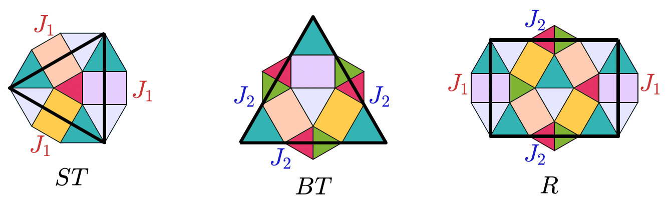
Figure 7. Two different types $J_{1},J_{2}$ of the boundaries of Bronze-means tiles

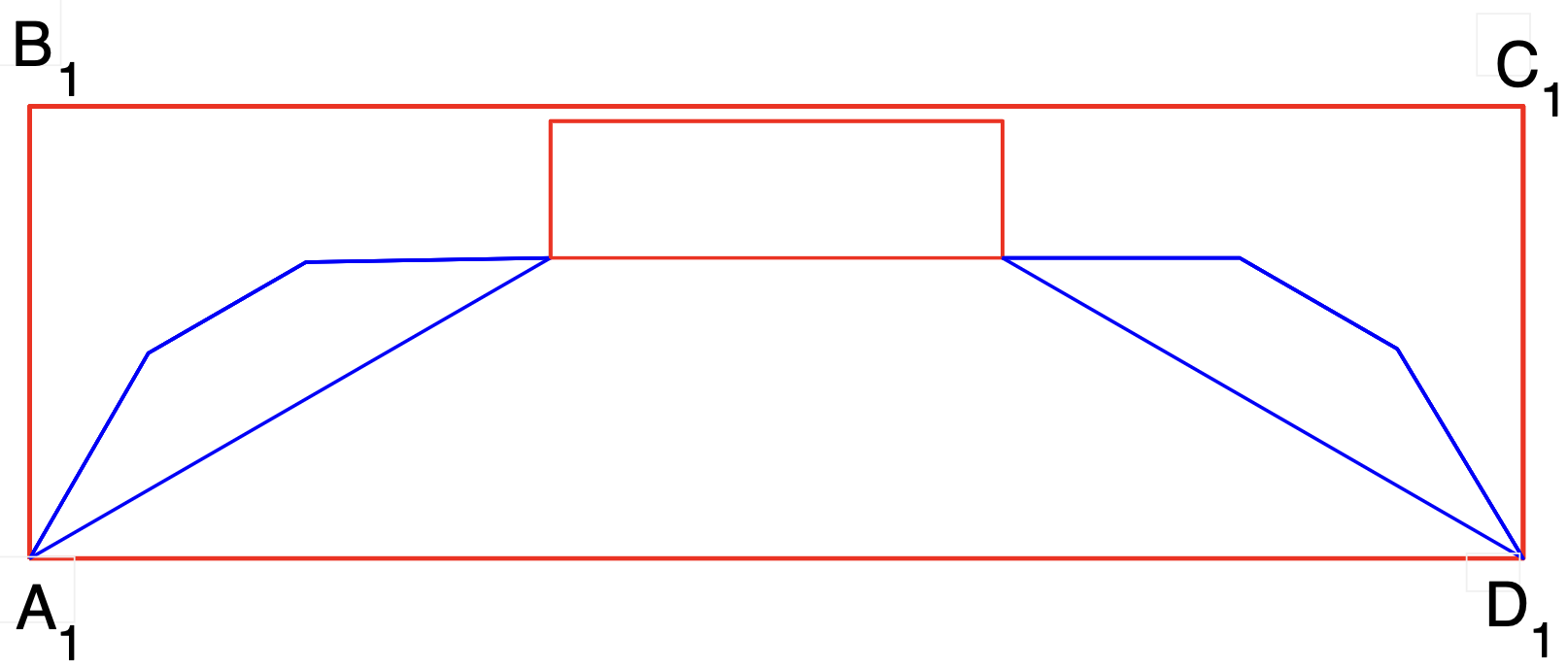
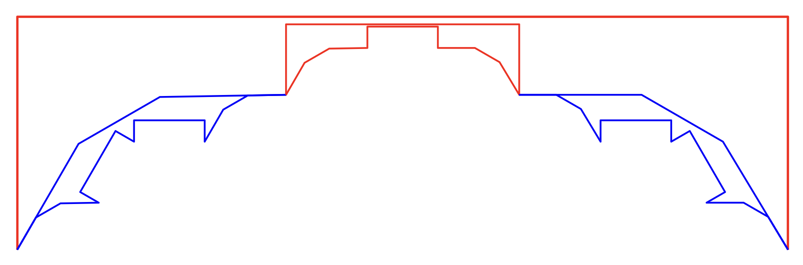
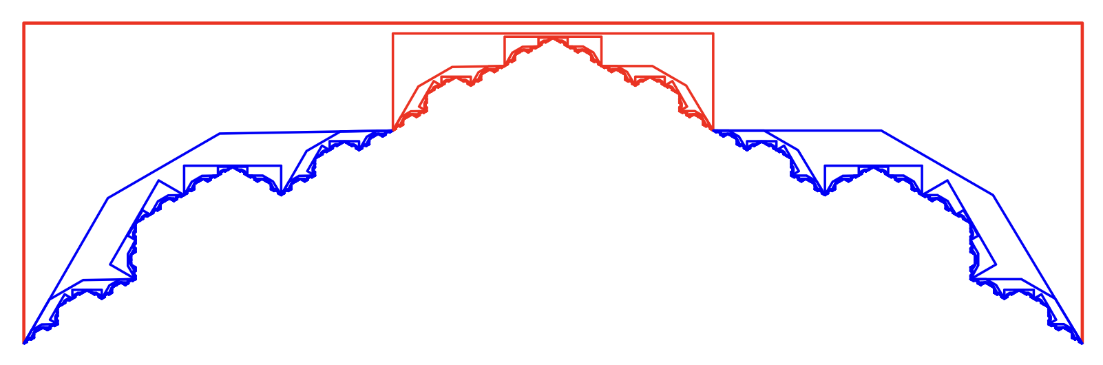
Figure 8. Feasible open sets for $J_{1}$: the interior of rectangle $A_{1}B_{1}C_{1}D_{1}$. To be safe, we show the coordinates which are $A_{1}=(0,0),B_{1}=(0,r),C_{1}=(1,r),D_{1}=(1,0)$, where $r=\frac{\sqrt{13}-3}{2}.$

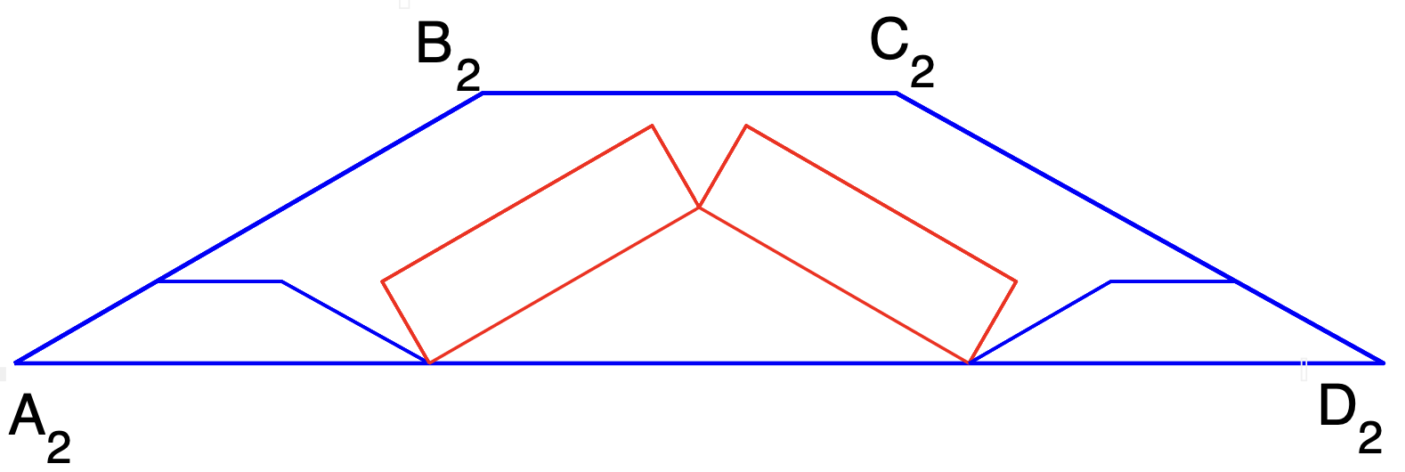
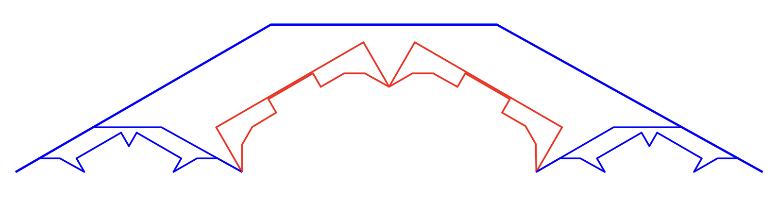
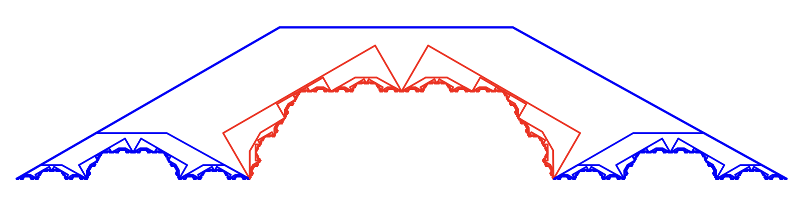
Figure 9. Feasible open sets for $J_{2}$: the interior of the isosceles trapezoid $A_{2}B_{2}C_{2}D_{2}$ with the coordinates $A_{2}=(0,0),B_{2}=(\frac{3}{2},\frac{\sqrt{3}}{2})r,C_{2}=(\frac{3}{2}+s,\frac{\sqrt{3}}{2})r,D_{2}=(s,0)$, here $s=\frac{r+2}{\sqrt{3}}$.

For the Bronze-mean tiles we introduced at beginning (See Figure 4), we will show here that the boundaries of tiles satisfy the open set condition and the feasible sets satisfy linear IFS condition.

Denote the Bronze-means tiles by $T_{1}$ (produced by $ST$), $T_{2}$ (produced by $BT$) and $T_{3}$ (produced by $R$). By the construction of $T_{1},T_{2}$ and $T_{3}$ , the boundaries of them are distinguished by two different types, say $J_{1}$ and $J_{2}$ (see Figure 7). And $J_{1}$, $J_{2}$ satisfy the following set equations

$$J_{1} =f_{12}(J_{2})\cup f_{11}(J_{1})\cup f_{12}^{\prime}(J_{2})$$

$$J_{2} =f_{22}(J_{2})\cup f_{21}(J_{1})\cup f_{21}^{\prime}(J_{1})\cup f_{22}^{\prime}(J_{2})$$

(Here $f_{ij}$ and $f_{ij}^{\prime}$ could be written through Figure 7.) Let $U_{1}$ be the rectangle $A_{1}B_{1}C_{1}D_{1}$ without the boundary in Figure 8 and $U_{2}$ be the trapezoid $A_{2}B_{2}C_{2}D_{2}$ without the boundary in Figure 9. Then we know $U_{1}$ and $U_{2}$ satisfy

$$f_{12}(U_{2})\cup f_{11}(U_{1})\cup f_{12}^{\prime}(U_{2}) \subset U_{1}$$

$$f_{22}(U_{2})\cup f_{21}(U_{1})\cup f_{21}^{\prime}(U_{1})\cup f_{22}^{\prime}(U_{2}) \subset U_{2}$$

To check the feasible open sets satisfying the linear GIFS condition, we take $U_{1}$ as an example, it is easy to see from Figure 8 and 9 that $\overline{f_{12}(U_{2})}\cap\overline{f_{11}(U_{1})}$ and $\overline{f_{11}(U_{1})}\cap\overline{f_{12}^{\prime}(U_{2})}$ are both singletons.

Example 4.2 (Feasible open sets for boundaries square triangle ’tiles’).

The square triangle is showing in Figure 3 and it is easy to know that they have fractal boundaries. We will present that the boundaries satisfy the open set condition and the feasible sets satisfy linear IFS condition.

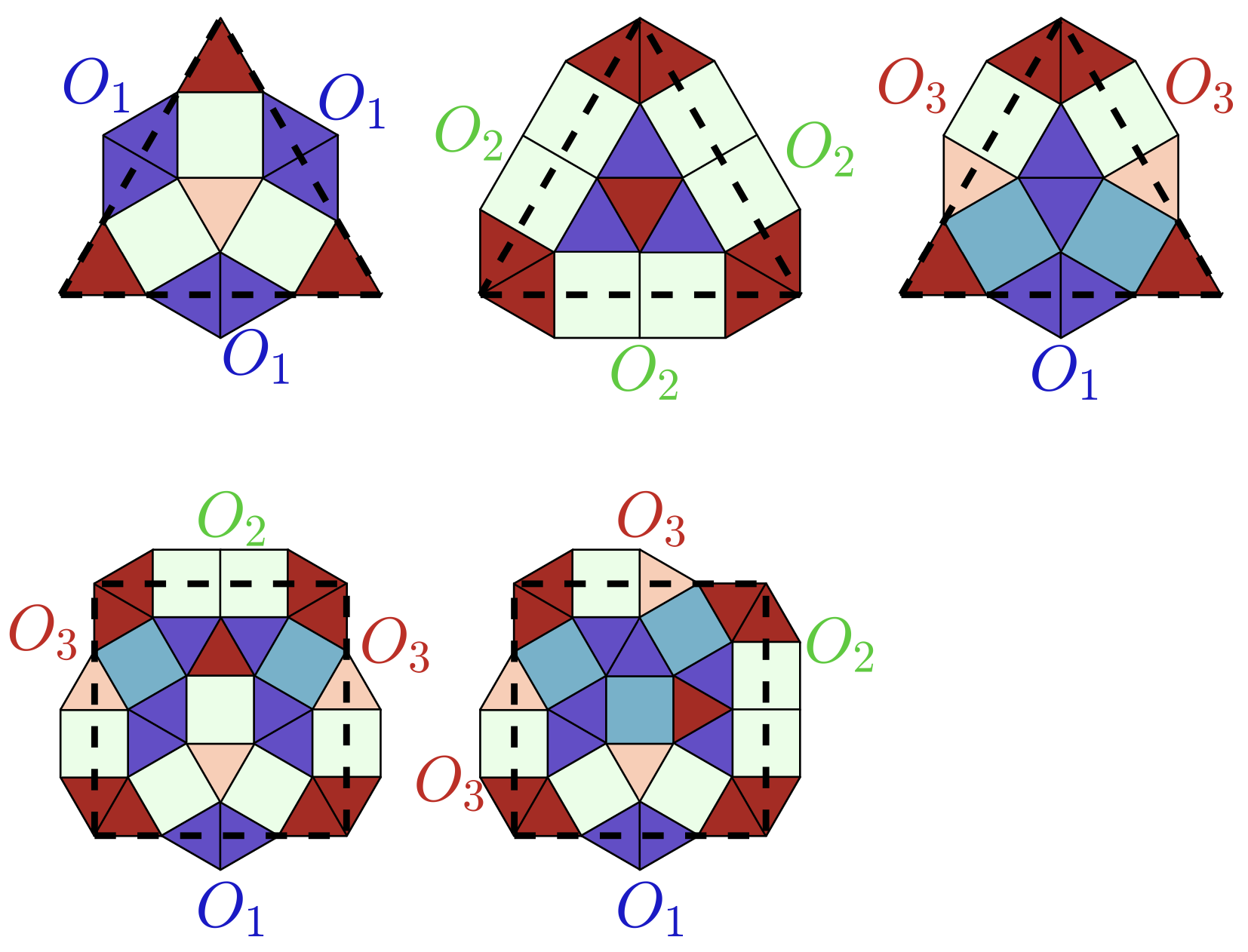
Figure 10. Three different types $O_{1},O_{2}$ and $O_{3}$ of the boundaries of square triangle tiles

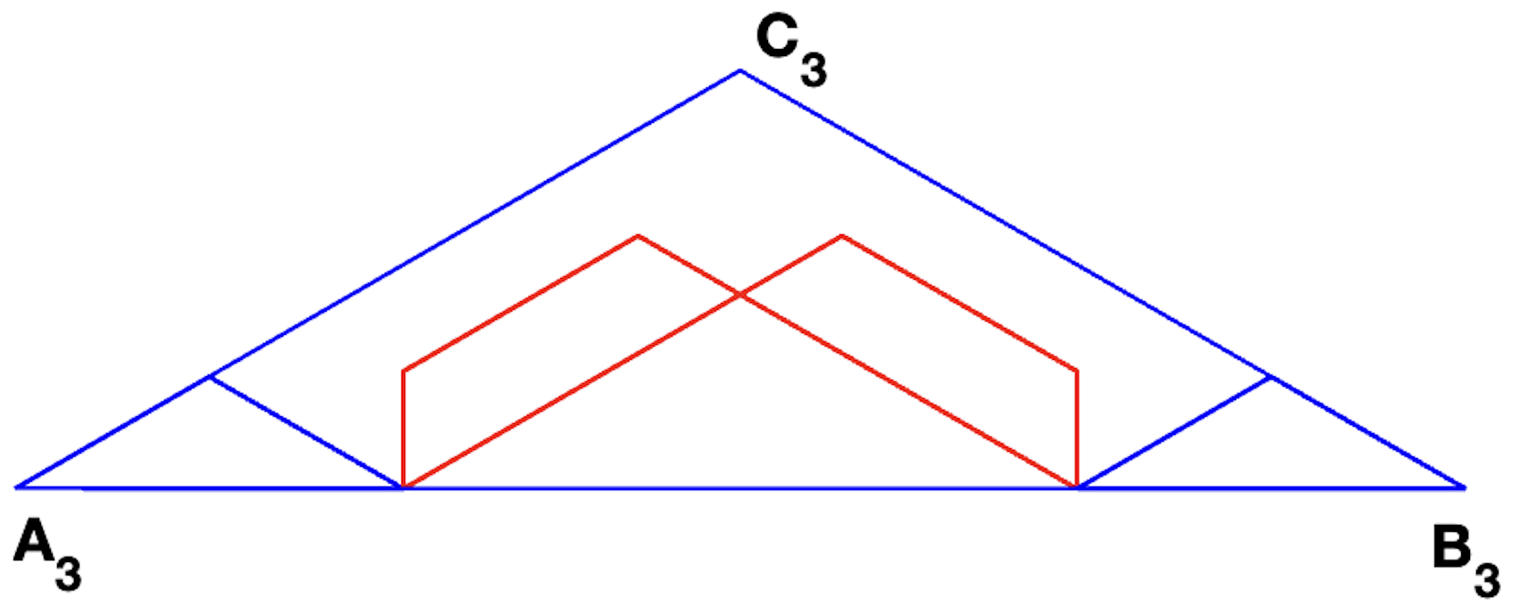
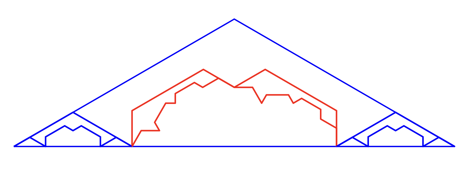
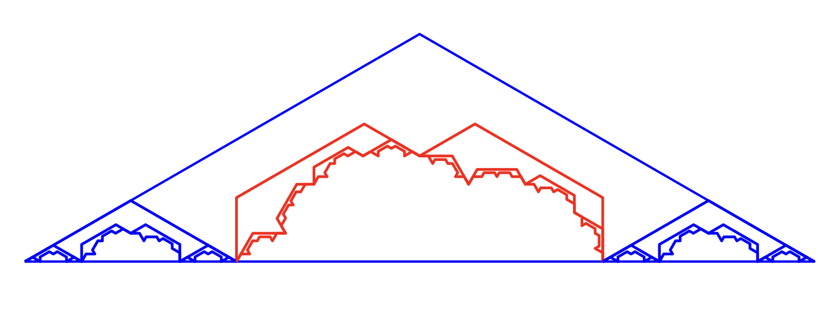
Figure 11. Feasible open set for $K_{1}$: the interior of the triangle which is an isosceles triangle with base angle is $\frac{\pi}{6}$ and length of base edge $1$.

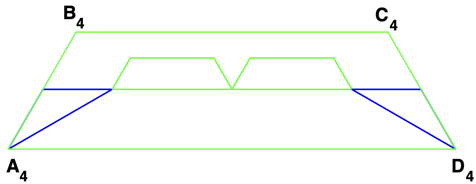
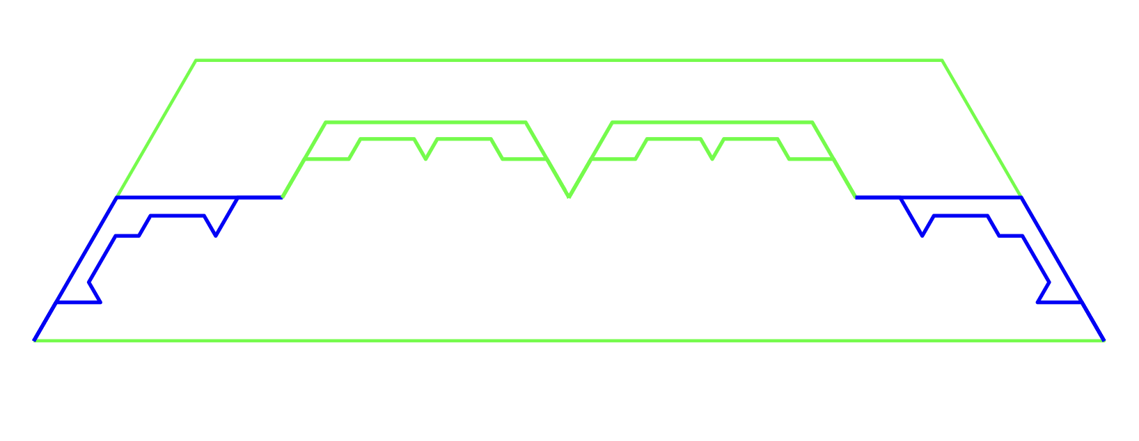
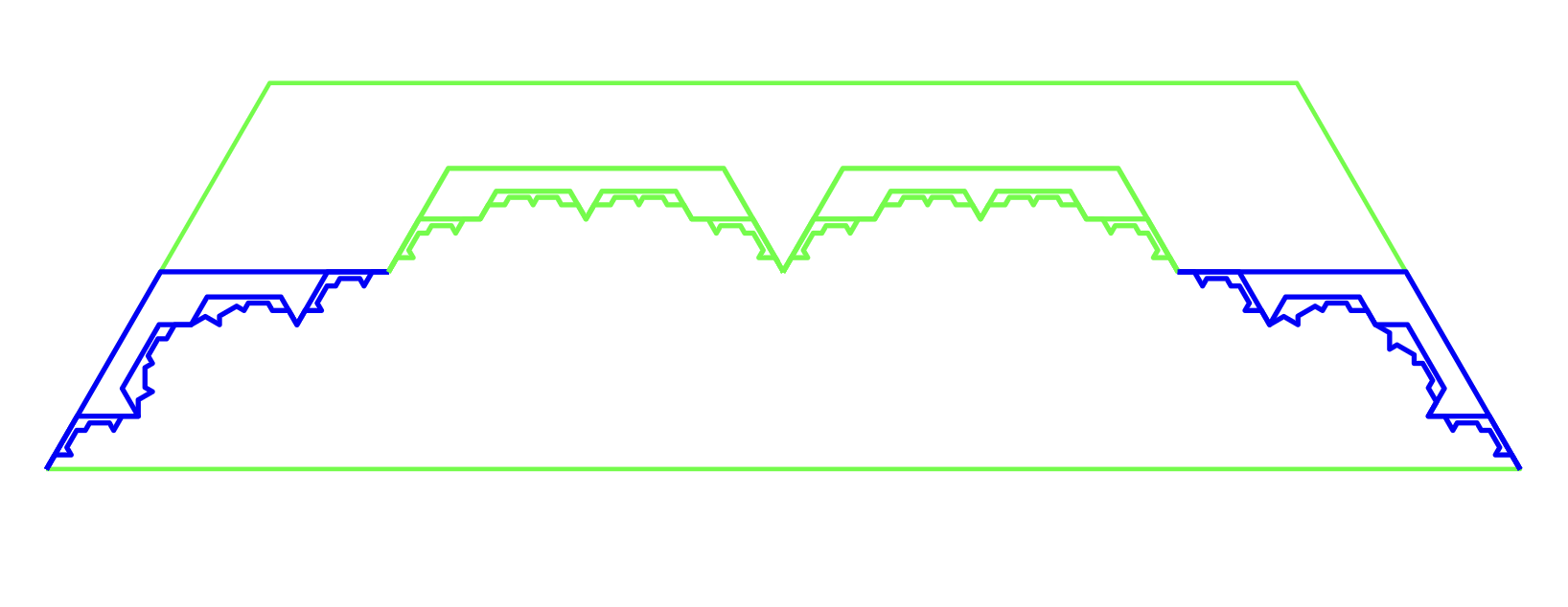
Figure 12. Feasible open set for $K_{2}$: the interior of an isosceles trapezoid with base angle $\frac{\pi}{3}$, base edge with length $1$ and equal edges with length $r=\frac{\sqrt{13}-3}{2}$.

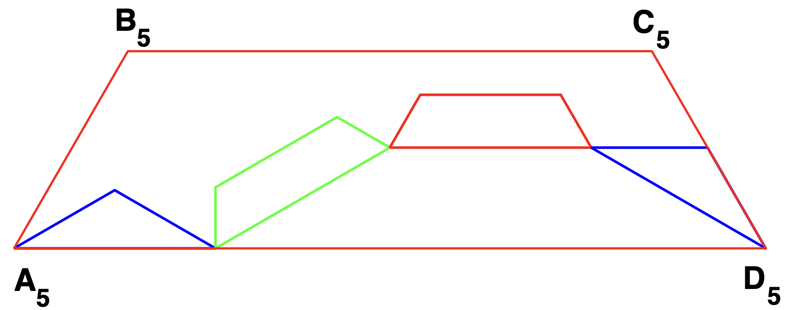
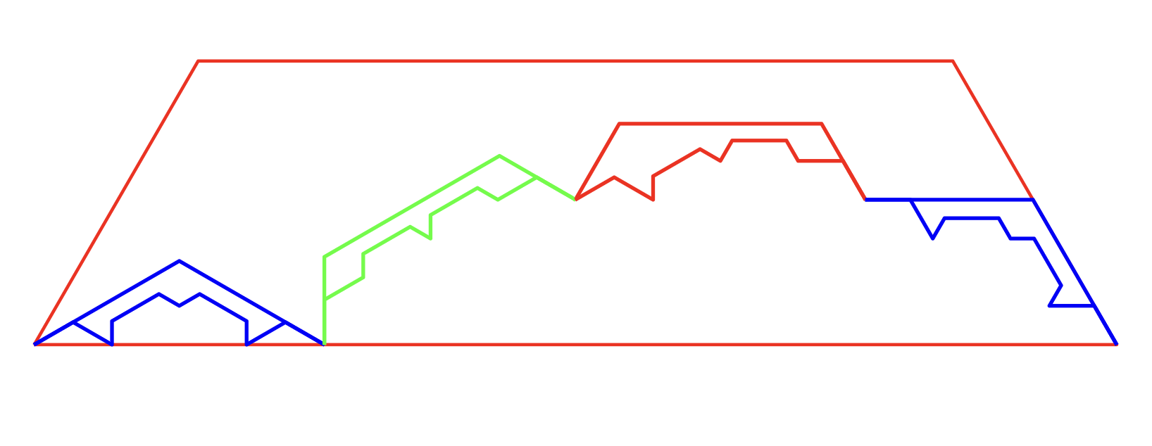
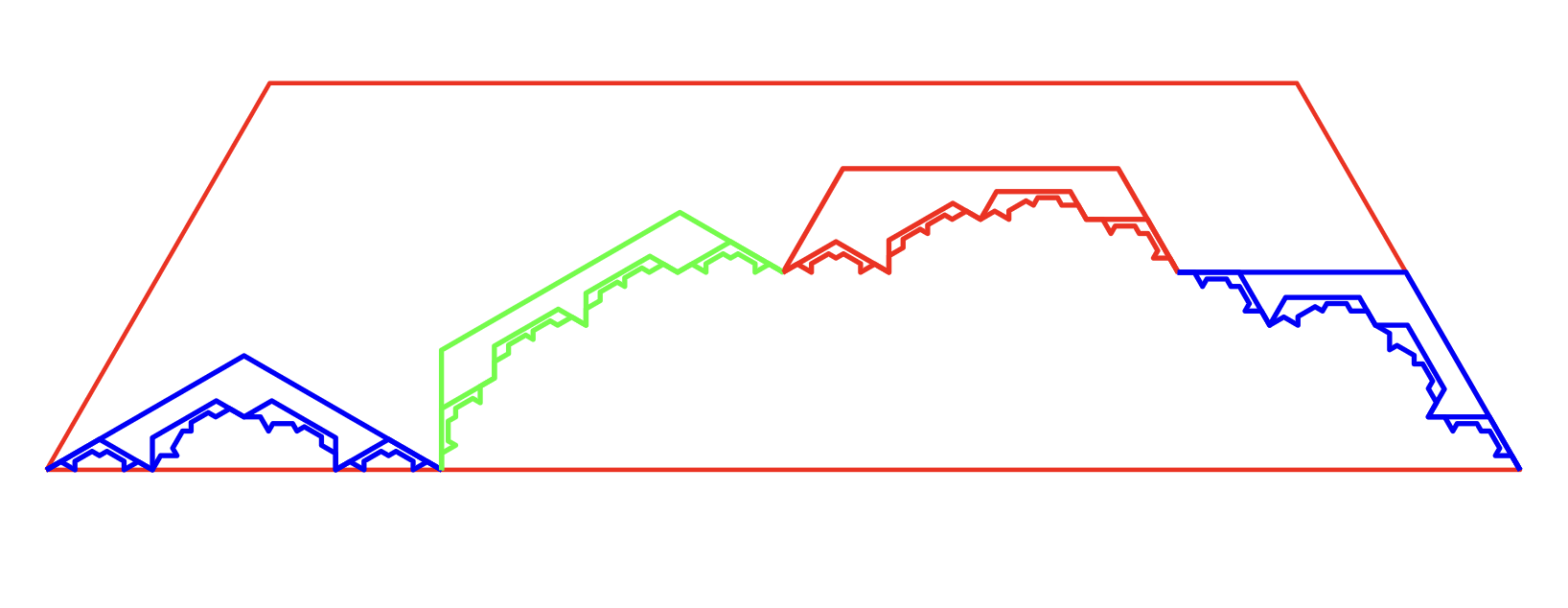
Figure 13. Feasible open set for $K_{3}$: the interior of the isosceles trapezoid same as above Figure 12.

Set the tiles related to square triangle tiling substitution by $T_{1},T_{2},T_{3}$ (produced by $Tr1,Tr2,Tr3$, respectively) and $T_{4},T_{5}$ (produced by $R1,R2$ respectively.) By the same idea with Bronze-mean tiles we know that the boundaries of $T_{i}$ could be classified by three different types $K_{1},K_{2}$ and $K_{3}$. And there exist set equations on $K_{i}$ for $i=1,2,3$ as follows.

$$K_{1} =g_{11}(K_{1})\cup g_{13}(K_{3})\cup g_{13}^{\prime}(K_{2})\cup g_{11}^{\prime}(K_{1}),$$

$$K_{2} =g_{21}(K_{1})\cup g_{22}(K_{2})\cup g_{22}^{\prime}(K_{2})\cup g_{21}^{\prime}(K_{1}),$$

$$K_{3} =g_{31}(K_{1})\cup g_{32}(K_{2})\cup g_{33}(K_{3})\cup g_{31}^{\prime}(K_{1}).$$

Let $O_{1}$ be the interior of triangle $A_{3}B_{3}C_{3}$ in Figure 11 and $O_{2}$ (and $O_{3}$) be the interior of the trapezoid $A_{4}B_{4}C_{4}D_{4}$ (and $A_{5}B_{5}C_{5}D_{5}$) in Figure 12 and 13. Thus $O_{1},O_{2}$ and $O_{3}$ have the following inclusion relations which show the open set condition and satisfy the linear IFS condition.

$$g_{11}(O_{1})\cup g_{13}(O_{3})\cup g_{13}^{\prime}(O_{2})\cup g_{11}^{\prime}(O_{1}) \subset O_{1},$$

$$g_{21}(O_{1})\cup g_{22}(O_{2})\cup g_{22}^{\prime}(O_{2})\cup g_{21}^{\prime}(O_{1}) \subset O_{2},$$

$$g_{31}(O_{1})\cup g_{32}(O_{2})\cup g_{33}(O_{3})\cup g_{31}^{\prime}(O_{1}) \subset O_{3}.$$

5. Construction of overlapping substitutions

5.1. A construction of one-dimensional overlapping substitutions

In this section, we show a way to construct interesting one-dimensional overlapping substitutions. The outline of the method consists of

1. find a “symbolic overlapping substitution” $\sigma$ with an alphabet $\mathcal{A}=\{1,2,\ldots,\kappa\}$, for which we draw graphs called adjacency graphs.

2. define the substitution matrix for the symbolic overlapping substitution $\sigma$.

3. assuming the substitution matrix is primitive, we compute the Perron–Frobenius eigenvalue $\beta$ and a Perron–Frobenius left eigenvector $(l_{1},l_{2},\ldots,l_{\kappa})$. Then consider a tile $T_{i}=([0,l_{i}],i)$. The set $\{T_{1},T_{2},\ldots,T_{\kappa}\}$ of these tiles becomes the alphabet for (geometric) overlapping substitution, which is obtained by juxtaposing these $T_{i}$’s in the same manner as the original symbolic overlapping substitution.

Step 1. A symbolic overlapping substitution $\sigma$ is a (symbolic) weighted substitution with an additional condition (c.f. [11]). A weighted substitution on an alphabet $\mathcal{A}$ is a rule which maps $a\in\mathcal{A}$ to a string

$$[a_{1}]_{r_{1}}[a_{2}]_{r_{2}}\cdots[a_{m}]_{r_{m}},$$

where $\kappa>0,a_{i}\in\mathcal{A}$ and $0<r_{i}\leqq 1$. We call such a map $\sigma$ a symbolic overlapping substitution if it satisfies conditions

1. if $m=1$, then $r_{1}=1$.

2. if $m>1$, then $r_{i}=1$ for any $1<i<m$.

We omit the corresponding bracket if $r_{i}$ is 1.

Example 5.1.

Let the alphabet $\mathcal{A}$ be $\{a,b,c\}$. Consider a rule $\sigma$ defined as

$$a\rightarrow[a]_{1/2}ba$$

$$b\rightarrow c[a]_{1/2}$$

$$c\rightarrow b[a]_{1/2}$$

We will draw adjacency graphs $G_{k}$, $k=1,2,\ldots$, as follows. They have the common vertex set $\mathcal{A}$. The edges are defined as follows. First, we draw an edge $e\rightarrow f$ for $e,f\in\mathcal{A}$ if $[e]_{r}[f]_{s}$ is a subword of the image of a letter by $\sigma$. The graph thus obtained is denoted by $G_{1}$.

Next, when we obtained $G_{k}$, we define $G_{k+1}$. In addition to edges in $G_{k}$, we draw an edge $e\rightarrow f$ if there is an edge $h\rightarrow g$ in $G_{k}$ such that $\sigma(h)$ ends with $[e]_{1}$ and $\sigma(g)$ starts with $[f]_{1}$.

The growing graphs $G_{1},G_{2}\ldots$ eventually stabilize and the final graph is called the adjacency graph $G$ for $\sigma$. This $G$ is said to be consistent if whenever $e\rightarrow f$ is an edge in $G$, we have either

• The last weight of $\sigma(e)$ and the first weight of $\sigma(f)$ are both 1, or

• The word $\sigma(e)$ ends with $[h]_{r}$ and $\sigma(f)$ starts with $[h]_{1-r}$, for some $h\in\mathcal{A}$ and $r\in(0,1)$.

We only consider symbolic overlapping substitutions with consistent adjacency graphs, since this is necessary for the consistency for the resulting geometric overlapping substitutions.

In practice, when we try to construct an example of geometric overlapping substitution by this way, we usually first construct a graph $G$ and then find a symbolic overlapping substitution with $G$ as a consistent adjacency graph.

Adjacency graphs for Example 5.1. By the definition of $G_{k}$, we have the $G_{1}$ and $G_{2}$ as in the following Figure 14. And $G_{3}=G_{2}$, then we have $G_{k}=G_{2}$ for all $k\geq 3$.

Figure 14. $G_{1},G_{2}$ and $G_{k}$ for $k\geq 3$.

Step 2. Given a symbolic overlapping substitution $\sigma$ with alphabet $\mathcal{A}=\{1,2,\ldots,\kappa\}$, we define its substitution matrix. It is a $\kappa\times\kappa$ matrix $M$ such that

$$M_{i,j}=\sum_{i\colon a_{i}=j}r_{i}$$

where the image of $j$ is written as

$$\sigma(j)=[a_{1}]_{r_{1}}[a_{2}]_{r_{2}}\cdots[a_{k}]_{r_{k}}.$$

In other words, we count the number of appearances of $i$ in the image of $j$, while regarding the appearance at the beginning or the end is counted by their weights.

The symbolic overlapping substitution is said to be primitive if its substitution matrix is primitive.

Substitution matrix for Example 5.1. The substitution matrix is given by

$$M=\begin{pmatrix}3/2&1/2&1/2\\ 1&0&1\\ 0&1&0\end{pmatrix}.$$

Step 3. Assume the substitution matrix $M$ for a symbolic overlapping substitution $\sigma$ is primitive. Let $\beta$ be the Perron–Frobenius eigenvalue and $(l_{1},l_{2},\ldots,l_{\kappa})$ be a Perron–Frobenius left eigenvector with positive entries. We construct a set of tiles $\{T_{1},T_{2},\ldots,T_{\kappa}\}$ by $T_{i}=([0,l_{i}],i)$. By definition, we have

$$\sum_{j=1}^{\kappa}\sum_{i\colon a_{i}=j}r_{i}l_{j}=\beta l_{k},$$

if

$$\sigma(k)=[a_{1}]_{r_{1}}[a_{2}]_{r_{2}}\cdots[a_{k}]_{r_{k}}.$$

We then define a (geometric) overlapping substitution $\rho$ by

$$\rho(T_{i})=\left\{T_{a_{1}},T_{a_{2}}+l_{a_{1}},\ldots,T_{a_{k}}+\sum_{j=1}^{k-1}l_{a_{j}}\right\}-(1-r)l_{a_{1}},$$

where

$$\sigma(i)=[a_{1}]_{r}a_{2}a_{3}\cdots a_{k-1}[a_{k}]_{s}.$$

In other words, we juxtapose the copies of alphabet by the order of $\sigma$ and translate every tile by $(1-r)l_{a_{1}}$, so that a part of the initial $T_{a_{1}}$ “sticks out” from the enlarged original tile $[0,\beta l_{i}]$ by the ratio $1-r$. We see a part of the final tile $T_{a_{k}}$ also “sticks out” from the enlarged tile $[0,\beta l_{i}]$ by the ratio $1-s$ (if $s<1$), by the computation

$$\beta l_{i}=rl_{a_{1}}+l_{a_{2}}+l_{a_{3}}+\cdots+l_{a_{k-1}}+sl_{a_{k}}.$$

The (geometric) overlapping substitution for Example 5.1. It is easy to know that the Perron–Frobenius eigenvalue of $M$ in Example 5.1 is $2$ and the corresponding left eigenvector is $(l_{a},l_{b},l_{c})=(2,1,1)$. Then we have

$$T_{a}=([0,l_{a}],1),T_{b}=([0,l_{b}],2)\text{ and }T_{c}=([0,l_{c}],3).$$

And the (geometric) overlapping substitution $\rho$ (see Figure 15) by

$$\left\{\begin{aligned} \rho(T_{a})&=\{[0,2],[0,1]+l_{a},[0,2]+l_{a}+l_{b}\}-(1-1/2)l_{a}=\{[-1,1],[1,2],[2,4]\}\\ \rho(T_{b})&=\{[0,1],[0,2]+l_{c}\}-(1-1)l_{c}=\{[0,1],[1,3]\}\\ \rho(T_{c})&=\{[0,1],[0,2]+l_{b}\}-(1-1)l_{b}=\{[0,1],[1,3]\}\end{aligned}\right.$$

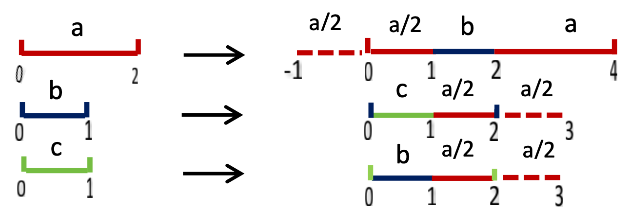
Figure 15. Geometric overlapping substitution

by

$$\left\{\begin{aligned} \sigma(a)&=[a]_{\frac{1}{2}}[b]_{1}[a]_{1}\\ \sigma(b)&=[c]_{1}[a]_{\frac{1}{2}}\\ \sigma(c)&=[b]_{1}[a]_{\frac{1}{2}}\end{aligned}\right.,$$

In the next proposition, we show that the (geometric) pre-overlapping substitution $\rho$ constructed in this way is consistent.

Proposition 5.2.

The pre-overlapping substitution $\rho$ is consistent.

Proof.

Define another graph $G^{\prime}_{k}$, $k=1,2,\ldots,$ as follows. The set of vertices for $G_{k}^{\prime}$ is $\mathcal{A}$. If for some $\nu=1,2,\ldots,k$ and $a\in\mathcal{A}$, a translate of the patch $\{T_{i},T_{j}+l_{i}\}$ appears in $\rho^{\nu}(T_{a})$, we draw an edge $i\rightarrow j$ for $G_{k}^{\prime}$. We see $G_{1}=G_{1}^{\prime}$. Let $k$ be an integer greater than 0. If $G_{k}=G_{k}^{\prime}$ and $\rho^{k}(T_{a})$ is consistent (that is, no illegal overlaps) for each $a\in\mathcal{A}$, then we can show that $G_{k+1}=G^{\prime}_{k+1}$ and $\rho^{k+1}(T_{a})$ is consistent for each $a\in\mathcal{A}.$ ∎

Example 5.3.

Let the alphabet $\mathcal{A}$ be $\{a,b,c,d\}$. Consider a rule $\sigma$ defined as  
$\sigma:\left\{\begin{aligned} a&\longrightarrow[a]_{r}bca\\ b&\longrightarrow bc\\ c&\longrightarrow d[a]_{1-r}\\ d&\longrightarrow[a]_{r}bc[a]_{1-r}\\ \end{aligned}\right.$ for any $0<r<1$.

Then the adjacent graphs determined by the above rule are drawn in Figure 16. By the definition, we know that $G_{k}=G_{2}$ for $k\geq 3$.

Figure 16. $G_{1},G_{2}$ and $G_{k}$ for $k\geq 3$.

The substitution matrix is

$$M=\left(\begin{matrix}1+r&0&1-r&1\\ 1&1&0&1\\ 1&1&0&1\\ 0&0&1&0\\ \end{matrix}\right).$$

And the characteristic polynomial is $P_{M}(x)=x^{4}-(2+r)x^{3}+(2r-1)x^{2}+rx$.
The Perron–Frobenius eigenvalue is $\beta=1+\sqrt{2}$ and the right eigenvector for $\beta$ is $(1-\frac{\sqrt{2}}{2},1-\frac{\sqrt{2}}{2},1-\frac{\sqrt{2}}{2},\frac{3\sqrt{2}}{2}-2)$ but the left eigenvector

$$(l_{a},l_{b},l_{c},l_{d})=\left(\frac{\beta}{\beta-r},\frac{\beta-r-1}{\beta-r},\sqrt{2}\frac{\beta-r-1}{\beta-r},1\right)$$

which varies by the parameter $r$. We take $r=\sqrt{2}/2$ as an example then the left eigenvector for $\beta$ is $(l_{a},l_{b},l_{c},l_{d})=(\sqrt{2},\sqrt{2}-1,2-\sqrt{2},1)$. Then we have

$$T_{a}=([0,l_{a}],1),T_{b}=([0,l_{b}],2),T_{c}=([0,l_{c}],3),T_{d}=([0,l_{d}],4).$$

So the (geometric) overlapping substitution $\rho$ by

$$\left\{\begin{aligned} \rho(T_{a})&=\{[0,l_{a}],[0,l_{b}]+l_{a},[0,l_{c}]+l_{a}+l_{b},[0,l_{a}]+l_{a}+l_{b}+l_{c}\}-(1-r)l_{a}\\ &=\{[1-\sqrt{2},1],[1,\sqrt{2}],[\sqrt{2},2],[2,2+\sqrt{2}]\}\\ \rho(T_{b})&=\{[0,l_{b}],[0,l_{c}]+l_{b}\}-(1-1)l_{b}=\{[0,\sqrt{2}-1],[\sqrt{2}-1,1]\}\\ \rho(T_{c})&=\{[0,l_{d}],[0,l_{a}]+l_{d}\}-(1-1)l_{d}=\{[0,1],[1,1+\sqrt{2}]\}\\ \rho(T_{d})&=\{[0,l_{a}],[0.l_{b}]+l_{a},[0,l_{c}]+l_{a}+l_{b},[0,l_{a}]+l_{a}+l_{b}+l_{c}\}-(1-r)l_{a}\\ &=\{[1-\sqrt{2},1],[1,\sqrt{2}],[\sqrt{2},2],[2,2+\sqrt{2}]\}\end{aligned}\right.$$

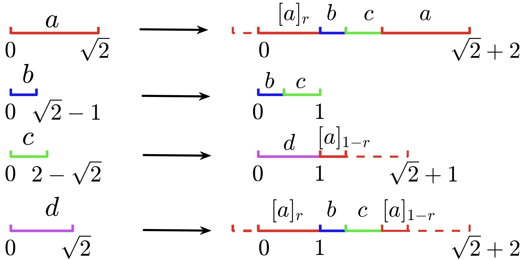
Figure 17. Geometric overlapping substitution for Example 5.3 when $r=\sqrt{2}/2$.

by

$$\left\{\begin{aligned} \sigma(a)&=[a]_{r}[b]_{1}[c]_{1}[a]_{1}\\ \sigma(b)&=[b]_{1}[c]_{1}\\ \sigma(c)&=[d]_{1}[a]_{1-r}\\ \sigma(d)&=[a]_{r}[b]_{1}[c]_{1}[a]_{1-r}\end{aligned}\right.,$$

here $r=\sqrt{2}/2$.

Example 5.4 (An example with two parameters).

Let the alphabet $\mathcal{A}$ be $\{a,b,c,d,e\}$. Consider a rule $\sigma$ defined as

$\sigma:\left\{\begin{aligned} a&\longrightarrow[c]_{1-s}abcade[a]_{r}\\ b&\longrightarrow[a]_{1-r}de[c]_{s}\\ c&\longrightarrow[c]_{1-s}ab[c]_{s}\\ d&\longrightarrow[a]_{1-r}d\\ e&\longrightarrow eab[c]_{s}\\ \end{aligned}\right.$ for any $0<r,s<1$.

By the above rule we have the adjacent graphs showing in Figure 18.

Figure 18. $G_{1}$ and $G_{k}$ for $k\geq 2$.

The substitution matrix is

$$M=\left(\begin{matrix}2+r&1-r&1&1-r&1\\ 1&0&1&0&1\\ 2-s&s&1&0&s\\ 1&1&0&1&0\\ 1&1&0&0&1\\ \end{matrix}\right).$$

So the characteristic polynomial with respect to $M$ is

$$P_{M}(x)=(r-x)(x-1)(x^{3}-4x^{2}-x+2),$$

and $\beta$ is the positive root $\approx 4.12$ of $x^{3}-4x^{2}-x+2=0$. A right eigenvector for $\beta$ is

$$(p,p-2,p^{2}-3p-2,2,2)$$

here we use $p=PF_{M}$ for simplicity. A left Perron–Frobenius eigenvector

$$(p^{2}(7-s)+ps-3,(p-1)\left(p^{2}(1-r)+p(r+s)-1\right),(p-1)p(p-r),$$

$$(1-r)\left(2p^{2}-ps+p-1\right),p(p-r)(p+s-1))$$

is a function on $r$ and $s$. Taking $r=s=1/2$ as an example, we have a left eigenvector

$$(l_{a},l_{b},l_{c},l_{d},l_{e})=(2\left(13p^{2}+p-6\right),2p(5p-3),2p(5p+3)-8,4p^{2}+p-2,p(12p+5)-8).$$

Then we have $T_{a}=([0,l_{a}],1),T_{b}=([0,l_{b}],2),T_{c}=([0,l_{c}],3),T_{d}=([0,l_{d}],4),T_{e}=([0,l_{e}],5).$ So we have the geometric overlapping substitution $\rho$ by $\sigma$ in the following way

$$\left\{\begin{aligned} \rho(T_{a})&=\{[0,l_{c}],[0,l_{a}]+l_{c},[0,l_{b}]+l_{a}+l_{c},[0,l_{c}]+l_{a}+l_{b}+l_{c},[0,l_{a}]+l_{c}+l_{a}+l_{b}+l_{c},\\ &[0,l_{d}]+2l_{c}+2l_{a}+l_{b},[0,l_{e}]+2l_{c}+2l_{a}+l_{b}+l_{d},[0,l_{a}]+2l_{c}+2l_{a}+l_{b}+l_{d}+l_{e}\}-sl_{c}\\ &=\{[-\frac{l_{c}}{2},\frac{l_{c}}{2}],[\frac{l_{c}}{2},l_{a}+\frac{l_{c}}{2}],[l_{a}+\frac{l_{c}}{2},l_{a}+l_{b}+\frac{l_{c}}{2}],[l_{a}+l_{b}+\frac{l_{c}}{2},l_{a}+l_{b}+\frac{3l_{c}}{2}],\\ &[l_{a}+l_{b}+\frac{3l_{c}}{2},2l_{a}+l_{b}+\frac{3l_{c}}{2}],[2l_{a}+l_{b}+\frac{3l_{c}}{2},2l_{a}+l_{b}+\frac{3l_{c}}{2}+l_{d}],\\ &[2l_{a}+l_{b}+\frac{3l_{c}}{2}+l_{d},2l_{a}+l_{b}+\frac{3l_{c}}{2}+l_{d}+l_{e}],[2l_{a}+l_{b}+\frac{3l_{c}}{2}+l_{d}+l_{e},3l_{a}+l_{b}+\frac{3l_{c}}{2}+l_{d}+l_{e}]\}\\ \rho(T_{b})&=\{[0,l_{a}],[0,l_{d}]+l_{a},[0,l_{e}]+l_{a}+l_{d},[0,l_{c}]+l_{a}+l_{d}+l_{e}\}-(1-(1-r))l_{a}\\ &=\{[-\frac{l_{a}}{2},\frac{l_{a}}{2}],[\frac{l_{a}}{2},\frac{l_{a}}{2}+l_{d}],[\frac{l_{a}}{2}+l_{d},\frac{l_{a}}{2}+l_{d}+l_{e}],[\frac{l_{a}}{2}+l_{d}+l_{e},\frac{l_{a}}{2}+l_{d}+l_{e}+l_{c}]\}\\ \rho(T_{c})&=\{[0,l_{c}],[0,l_{a}]+l_{c},[0,l_{b}]+l_{c}+l_{a},[0,l_{c}]+l_{c}+l_{a}+l_{b}\}-(1-(1-s))l_{c}\\ &=\{[-\frac{l_{c}}{2},\frac{l_{c}}{2}],[\frac{l_{c}}{2},\frac{l_{c}}{2}+l_{a}],[\frac{l_{c}}{2}+l_{a},\frac{l_{c}}{2}+l_{a}+l_{b}],[\frac{l_{c}}{2}+l_{a}+l_{b},\frac{3l_{c}}{2}+l_{a}+l_{b}]\}\\ \rho(T_{d})&=\{[0,l_{a}],[0,l_{d}]+l_{a},\}-(1-(1-r))l_{a}=\{[-\frac{l_{a}}{2},\frac{l_{a}}{2}],[\frac{l_{a}}{2},\frac{l_{a}}{2}+l_{d}]\}\\ \rho(T_{e})&=\{[0,l_{e}],[0,l_{a}]+l_{e},[0,l_{b}]+l_{e}+l_{a},[0,l_{c}]+l_{e}+l_{a}+l_{b}\}-(1-1)l_{a}\\ &=\{[0,l_{e}],[l_{e},l_{a}+l_{e}],[l_{a}+l_{e},l_{a}+l_{b}+l_{e}],[l_{a}+l_{b}+l_{e},l_{a}+l_{b}+l_{c}+l_{e}]\}\end{aligned}\right.$$

here $\left\{\begin{aligned} \sigma(a)&=[c]_{\frac{1}{2}}abcade[a]_{\frac{1}{2}}\\ \sigma(b)&=[a]_{\frac{1}{2}}de[c]_{\frac{1}{2}}\\ \sigma(c)&=[c]_{\frac{1}{2}}ab[c]_{\frac{1}{2}}\\ \sigma(d)&=[a]_{\frac{1}{2}}d\\ \sigma(e)&=eab[c]_{\frac{1}{2}}\\ \end{aligned}\right.$

5.2. Construction from Delone sets with inflation symmetry

In this section, we construct overlapping substitutions from Delone (multi)sets with inflation symmetry. The idea is that, if a Delone (multi)set $X$ has inflation symmetry, then the corresponding Voronoi tiling must also have one and yields an overlapping substitution. A similar idea to construct a self-similar tiling from a point set satisfying a set equation is found in [6] in one-dimensional setting. Note also that [16] gave a construction of substitution from a tiling with inflation symmetry. Our construction is weaker in the sense that the substitutions constructed are overlapping, but stronger in the sense that the tiles are polygonal. (In [16], tiles are not necessarily connected.) The main theorem is Theorem 5.9 and the reader can omit the technical proofs for the first reading.

We fix a positive integer $d>0$ and an invertible linear map $A\colon\mathbb{R}^{d}\rightarrow\mathbb{R}^{d}$. We assume that for any $a,b\in\mathbb{R}$, there exists $L$ such that $A(B_{L+a})\supset B_{L+b}$ holds. We also set

$$H_{x,y}=\{z\in\mathbb{R}^{d}\mid\|x-z\|\leqq\|y-z\|\}$$

for each $x,y\in\mathbb{R}^{d}$.

For a function $f$ on $\mathbb{R}^{d}$ and $K\subset\mathbb{R}^{d}$, we define a cutting-off operation via

$$(f\wedge K)(x)=\begin{cases}f(x)&\text{ if $x\in K$}\\ 0&\text{ otherwise}.\end{cases}$$

We also define $Af$ via $(Af)(x)=f(A^{-1}x)$.

A cutting-off operation for patches is defined as follows:

$$\mathcal{P}\wedge K=\{T\in\mathcal{P}\mid\operatorname{supp}T\cap K\neq\emptyset\},$$

where $\mathcal{P}$ is a patch in $\mathbb{R}^{d}$ and $K\subset\mathbb{R}^{d}$.

We take a non-empty convex subset $\Omega\subset\mathbb{R}^{d}$ such that $A\Omega=\Omega$. We also take a Delone multiset $(X_{i})_{i=1}^{n}$ in $\Omega$. This means that each $X_{i}$ is a discrete subset with multiplicity, that is, there is a map $m_{i}\colon\mathbb{R}^{d}\rightarrow\mathbb{Z}_{\geqq 0}$ such that $\operatorname{supp}m_{i}=\underline{X_{i}}$ is a locally finite subset of $\Omega$, and $X=\bigcup_{i=1}^{n}\underline{X_{i}}$ is relatively dense with respect to an $R_{0}>0$ in $\Omega$. We assume $(X_{i})_{i}$ is locally derivable from $(AX_{i})_{i}$, which means that there is an $R_{D}>0$ such that if $x,y\in\mathbb{R}^{d}$ and

$$(Am_{i}-x)\wedge B_{R_{D}}=(Am_{i}-y)\wedge B_{R_{D}}$$

for each $i$, then we have $m_{i}(x)=m_{i}(y)$ for each $i$. For example, if there exist a family of finite sets $D_{ij}\subset\mathbb{R}^{d}$ and we have

$$X_{j}=\bigcup_{i=1}^{n}\bigcup_{d\in D_{ij}}AX_{i}+d,$$

with multiplicity, in other words, we have

$$m_{j}(x)=\sum_{i=1}^{n}\sum_{d\in D_{ij}}m_{i}(A^{-1}(x-d))$$

for each $j$ and $x$, then we have the local derivability. We set $M=(m_{i})_{i=1}^{n}$.

We construct an overlapping substitution from such a Delone multiset. For this purpose, we take three constants $R_{1},R_{2},R_{3}$ as follows: $R_{1}>0$ is such that $B_{R_{1}}\supset AB_{R_{0}+1}$; $R_{2}>0$ is such that $AB_{R_{2}}\supset B_{R_{1}+2R_{0}+2}$ and $AB_{R_{2}}\supset B_{R_{0}+R_{1}+R_{2}+1}$; $R_{3}=\max\{2R_{0}+2,R_{0}+R_{2}+1\}$.

For each $x\in X$, we set the Voronoi cell by

$$V_{x}=\{y\in\Omega\mid\text{$\|x-y\|\leqq\|y-z\|$ for any $z\in X\setminus\{x\}$}\}.$$

Take an $L>0$ and $x\in X$, and define a labeled tile $T_{x,L}$ via

$$T_{x,L}=(V_{x},((m_{i}-x)\wedge B_{L})_{i},V_{x}-x,(\Omega-x)\cap B_{R_{2}}).$$

Here, $V_{x}$ is the support of the tile and the rest are labels.

We set Voronoi tiling $\mathcal{T}_{L}$ via

$$\mathcal{T}_{L}=\{T_{x,L}\mid x\in X\}.$$

Lemma 5.5.

For each $x\in X$, we have

$$V_{x}=\bigcap_{y\in X\cap B(2R_{0}+2)}H_{x,y}\cap\Omega$$

and

$$V_{x}\subset B(x,R_{0}+1).$$

Proof.

We note that for each $y$, the set $H_{x,y}$ is convex. If we take an arbitrary

$$z\in U_{x}=\bigcap_{y\in X\cap B(x,2R_{0}+2)}H_{x,y}\cap\Omega,$$

we must have $\|x-z\|\leqq R_{0}+1$. Indeed, if we have $\|x-z\|>R_{0}+1$, we can take an appropriate $t\geqq 0$ such that $w=x+t(z-x)$ satisfies $\|x-w\|=R_{0}+1$. There is a $u\in B(w,R_{0})\cap X$ and we necessarily have $\|w-u\|<\|x-w\|$, and so $w\notin U_{x}$, contradicting the fact that $U_{x}$ is convex. Therefore, $U_{x}\subset B(x,R_{0}+1)$.

Take a $z\in U_{x}$. If $v\in X$ and $\|v-x\|>2R_{0}+2$, then we must have $\|z-u\|>\|x-z\|$, and so the claim follows. ∎

We set $R_{L}=\max\{3R_{0}+3,L+R_{0}+1\}$.

We have several lemmas on local derivability, as follows.

Lemma 5.6.

For each $L$, the tiling $\mathcal{T}_{L}$ is locally derivable from $(M,\Omega)$. In particular, if $x,y\in\mathbb{R}^{d}$,

$$(\Omega-x)\cap B_{R_{3}}=(\Omega-y)\cap B_{R_{3}},$$

and

$$(M-x)\wedge B_{R_{L}}=(M-y)\wedge B_{R_{L}},$$

then we have

$$(\mathcal{T}_{L}-x)\wedge\{0\}=(\mathcal{T}_{L}-y)\wedge\{0\}.$$

Proof.

If $z\in X$ and $T_{z,L}-x$ contains $0$, then by Lemma 5.5, we have $\|z-x\|\leqq R_{0}+1$, and so $z-x+y\in X$. We have

$$V_{z}-x =\left(\bigcap_{w\in X\cap B(z,2R_{0}+2)}H_{z,w}\cap\Omega\cap B(z,R_{0}+1)\right)-x$$

$$=\bigcap_{w\in(X-x)\cap B(z-x,2R_{0}+2)}H_{z-x,w}\cap(\Omega-x)\cap B(z-x,R_{0}+1)$$

By the assumption of the lemma, we have

$$(X-x)\cap B(z-x,2R_{0}+2) =(X-x)\cap B(0,R_{L})\cap B(z-x,2R_{0}+2)$$

$$=(X-y)\cap B(0,R_{L})\cap B(z-x,2R_{0}+2)$$

$$=(X-y)\cap B(z-x,2R_{0}+2),$$

and

$$(\Omega-x)\cap B(z-x,R_{0}+1) =(\Omega-x)\cap B(0,2R_{0}+2)\cap B(z-x,R_{0}+1)$$

$$=(\Omega-y)\cap B(0,2R_{0}+2)\cap B(z-x,R_{0}+1)$$

$$=(\Omega-y)\cap B(z-x,R_{0}+1),$$

and so

$$V_{z}-x=\left(\bigcap_{w\in X\cap B(y+z-x,2R_{0}+2)}H_{y+z-x,w}\cap\Omega\cap B(y+z-x,R_{0}+1)\right)-y=V_{y+z-x}-y.$$

Moreover, we have

$$(m_{i}-z)\wedge B_{L}=(m_{i}+x-y-z)\wedge B_{L},$$

and

$$(\Omega-z)\cap B_{R_{2}}=(\Omega+x-y-z)\cap B_{R_{2}}.$$

We have proved

$$T_{z,L}-x=T_{y+z-x}-y,$$

and so $(\mathcal{T}_{L}-x)\wedge\{0\}\subset(\mathcal{T}_{L}-y)\wedge\{0\}$. By symmetry, the converse inclusion also follows. ∎

Corollary 5.7.

If $R^{\prime}>0$, $x,y\in\mathbb{R}^{d}$,

$$(\Omega-x)\cap B_{R^{\prime}+R_{3}}=(\Omega-y)\cap B_{R^{\prime}+R_{3}},$$

and

$$(M-x)\wedge B_{R^{\prime}+R_{L}}=(M-y)\wedge B_{R^{\prime}+R_{L}},$$

then we have

$$(\mathcal{T}_{L}-x)\wedge B_{R^{\prime}}=(\mathcal{T}_{L}-y)\wedge B_{R^{\prime}}.$$

Lemma 5.8.

For each $L>0$, if $x,y\in\mathbb{R}^{d}$ and

$$(\mathcal{T}_{L}-x)\wedge\{0\}=(\mathcal{T}_{L}-y)\wedge\{0\},$$

then we have

$$(M-x)\wedge B_{L-R_{0}-1}=(M-y)\wedge B_{L-R_{0}-1}.$$

Consequently,if $x,y\in\mathbb{R}^{d}$, $R^{\prime}>0$ and

$$(\mathcal{T}_{L}-x)\wedge B_{R^{\prime}}=(\mathcal{T}_{L}-y)\wedge B_{R^{\prime}},$$

then we have

$$(M-x)\wedge B_{R^{\prime}+L-R_{0}-1}=(M-y)\wedge B_{R^{\prime}+L-R_{0}-1}.$$

Proof.

Take a tile $T_{z,L}-x=T_{w,L}-y$ from the set $(\mathcal{T}_{L}-x)\wedge\{0\}=(\mathcal{T}_{L}-y)\wedge\{0\}$. We have $V_{z}-z=V_{w}-w$ and $V_{z}-x=V_{w}-y$. This means $x-y=z-w$. Combined with the fact that

$$(m_{i}-z)\wedge B_{L}=(m_{i}-w)\wedge B_{L},$$

for each $i$, we have

$$(m_{i}-x)\wedge B_{L-R_{0}-1} =(((m_{i}-z)\wedge B_{L})-x+z)\wedge B_{L-R_{0}-1}$$

$$=(((m_{i}-w)\wedge B_{L})-y+w)\wedge B_{L-R_{0}-1}$$

$$=(m_{i}-y)\wedge B_{L-R_{0}-1}.(m_{i}-y)\wedge B_{L-R_{0}-1}$$

for each $i$. ∎

Theorem 5.9.

If $L$ is large enough so that

$$AB_{L-R_{0}-1}\supset B_{R_{1}+R_{L}+R_{D}},$$

let us define an alphabet $\mathcal{A}$ via

$$\mathcal{A}=\{T_{x,L}-x\mid x\in X\}.$$

Then a map

$$\rho(T_{x,L}-x)=\mathcal{T}_{L}\wedge A(\operatorname{supp}T_{x,L})-A(x)$$

is well-defined and $(\mathcal{A},A,\rho)$ is a consistent overlapping substitution (with possibly an infinite alphabet).

Moreover

$$\rho(\mathcal{T}_{X,L})=\mathcal{T}_{X,L}.$$

Proof.

If $T_{x,L}-x=T_{y,L}-y$, then we have

$$(\mathcal{T}_{L}-x)\wedge\{0\}=(\mathcal{T}_{L}-y)\wedge\{0\},$$

and by Lemma 5.8,

$$(M-x)\wedge B_{L-R_{0}-1}=(M-y)\wedge B_{L-R_{0}-1}.$$

This means that

$$(AM-Ax)\wedge AB_{L-R_{0}-1}=(AM-Ay)\wedge AB_{L-R_{0}-1},$$

and so

$$(M-Ax)\wedge B_{R_{1}+R_{L}}=(M-Ay)\wedge B_{R_{1}+R_{L}},$$

by the inflation symmetry for $M$. Moreover, we have $(\Omega-Ax)\wedge B_{R_{1}+R_{3}}=(\Omega-Ay)\wedge B_{R_{1}+R_{3}}$. By Corollary 5.7, we have

$$(\mathcal{T}_{L}-x)\wedge B_{R_{1}}=(\mathcal{T}_{L}-y)\wedge B_{R_{1}},$$

from which the claim follows. ∎

Remark 5.1.

The tiles have many labels, but the last one can be removed by considering only $x\in X$ that is “inside” $\Omega$. After such a removal, if $X$ has finite local complexity, then $\mathcal{A}$ is finite.

Remark 5.2.

The construction in Theorem 5.9 is intended to be for Delone multi-sets with inflation symmetry and finite local complexity (FLC). If $\lambda$ is a Pisot number and $m$ is an integer with $m\geqq\lambda-1$, then the spectrum

$$X=\left.\left\{\sum_{j=0}^{n}\varepsilon_{j}\lambda^{j}\right|n\in\mathbb{Z}_{\geqq 0},\varepsilon_{j}\in\{-m,-m+1,\ldots,m-1,m\}\right\}$$

is an example of substitution (non-multi) Delone set in $\mathbb{R}$ with one color for $A(x)=\lambda x$.

6. Further problems

Self-similar tiling gives an associated IFS. Our definition of overlapping substitution is pretty restricted to the cases where the overlap happens only around the boundary of expanded pieces. Considering the associated IFS problems with overlaps, we discussed only the lucky cases. The problem of Bernoulli convolution deals with heavy overlaps (c.f. [18]), and it is challenging to extend our method.

P. Gummelt [10] gave a single decagon with special markings, which covers the plane but only in non-periodic ways. This covering encodes a version of Penrose tiling by Robinson’s triangle. This covering uses overlaps of pieces but it does not fall into our framework. It is interesting to have a possible generalization of overlap tiling, which includes such an example.

The construction in Theorem 5.9 is valid for Delone (multi) sets with inflation symmetry for $Ax=\lambda x$, where $\lambda$ is a Pisot number. However, it is not only for such cases and similar construction is possible for arbitrary real number $\lambda>1$. For the one-dimension case ($d=1$), we set $\Omega=[0,\infty)$, in order to avoid getting a non-discrete subset of $\mathbb{R}$. Fix an integer $m\geqq\lambda-1$. We set

$$X=\left.\left\{\sum_{j=0}^{n}\varepsilon_{j}\lambda^{j}\right|n\in\mathbb{Z}_{\geqq 0},\varepsilon_{j}\in\{0,1,\ldots,m-1,m\}\right\}$$

$X$ is a discrete subset of $\Omega$ that satisfies an equation

$$X=\bigcup_{i=0}^{m}\lambda X+i.$$

By the construction in Theorem 5.9, we can get an overlapping substitution $\rho$. In the case of non-Pisot $\lambda$, the set $X$ does not have finite local complexity and the alphabet forms an infinite set. However, $\rho$ have “continuity”, in the sense that if $P,Q$ in the alphabet are “close” (the supports and labels are close with respect to Hausdorff metric), then the resulting patches are “close” (each tile in one patch has a counterpart in the other which is “close”). Recently, substitutions with infinite alphabet has been paid attention. For example, [8] constructed substitutionis with compact infinite alphabet for arbitrary real number $\lambda>2$ as the inflation factor. Our method is significantly different from [8] but also enable us to construct substitutions with arbitrary $\lambda>1$ as the inflation factor.

We conjecture that, for an appropriate choice of a finite subset $F$ of $\mathbb{R}^{d}$, an expansive linear map $A$ on $\mathbb{R}^{d}$, and $\Omega=\{\sum_{f\in F}t_{f}f\mid t_{f}>0\}$,

$$\left\{\sum_{n=1}^{N}A^{n}a_{n}\mid N=1,2,\ldots,a_{n}\in F\right\}$$

is a Delone set of $\Omega$ with inflation symmetry and we will have a corresponding overlapping substitution. In high dimensions, few examples of substitutions are known, but this may give us many overlapping substitutions in such dimensions.

The family of overlapping substitutions with one or two parameters in Section 5.1 are examples of deformation of substitutions. Deformations of tilings are discussed in [4] and some of the deformations of a fixed point of a substitution are fixed points of deformed substitutions. It is interesting to investigate the nature of such special deformations.

7. Appendix

Here, we prove Proposition 2.6.

7.1. Notation

First, we fix notation. Let $v$ be a weighted pattern such that $\operatorname{SP}(v)$ is a tilig and $v(T)=1$ for each $T\in\operatorname{SP}(v)$. We assume $v$ is a fixed point for an iterate of a weighted substitution $\xi$, so that there is a $k>0$ such that $\xi^{k}(v)=v$. Let $\mathcal{B}=\{T_{1},T_{2},\ldots,T_{\kappa}\}$ be the alphabet for $\xi$ and $\phi$ be its expansion map. The substitution matrix for $\xi$ is denoted by $M$. We take a left Perron–Frobenius left eigenvector $\mathbf{l}=(l_{1},l_{2},\ldots,l_{\kappa})$ and right eigenvector $\mathbf{r}={}^{t}(r_{1},r_{2},\ldots,r_{\kappa})$ which are normalized in the sense that

$$\sum_{i=1}^{n_{1}}l_{i}r_{i}=\sum_{i=1}^{\kappa}r_{i}=1.$$

By taking similitude of proto-tiles if necessary, we may assume that

$$l_{i}=\operatorname{vol}(T_{i})$$

holds for each $i$.

For a weighted pattern $u$ with finite support patch, we set

$$\operatorname{vol}(u)=\sum_{T\in\operatorname{SP}(u)}u(T)\operatorname{vol}(T).$$

In what follows, we consider averaging over van Hove sequences in $\mathbb{R}^{d}$, and it is important to divide an element $A$ of a van Hove sequence into “interior” and “boundary”. For each $L>0$, we set

$$A^{-L} =\{t\in\mathbb{R}^{d}\mid B(t,L)\subset A\},$$

$$\partial^{L}A =\{t\in\mathbb{R}^{d}\mid B(t,L)\cap A\neq\emptyset,B(t,L)\cap A^{c}\neq\emptyset\}.$$

We also consider subsets of a patch $\operatorname{SP}(v)$, as follows, depending on whether the inflation of a tile in $\operatorname{SP}(v)$ is inside or not in side of $A$, and on the “boundary” of $A$:

$$\mathcal{P}(m,\subset A)=\{T\in\operatorname{SP}(v)\mid\operatorname{SR}(\xi^{km}(T))\subset A\},$$

$$\mathcal{P}(m,\not\subset A)=\{T\in\operatorname{SP}(v)\mid\operatorname{SR}(\xi^{km}(T))\not\subset A\},$$

$$\mathcal{P}(m,\partial A)=\{T\in\operatorname{SP}(v)\mid\operatorname{SR}(\xi^{km}(T))\not\subset A,\operatorname{SR}(\xi^{km}(T))\cap A\neq\emptyset\}.$$

Finally, for each natural number $m$, let $L_{m}$ be the maximal diameter for the region $\operatorname{SR}(\xi^{km}(T_{i}))$, $i=1,2,\ldots,\kappa$.

7.2. Proof

Lemma 7.1.

We have

$$\sum_{T\in\mathcal{P}(m,\subset A)}\tau_{T_{i}}(\xi^{km}(T))\leqq\tau_{T_{i}}(v\wedge A).$$

Proof.

For $T\in\mathcal{P}(m,\subset A)$, we have $\xi^{km}(T)=\xi^{km}(T)\wedge A$, and so

$$\tau_{T_{i}}\left(\sum_{T\in\mathcal{P}(m,\subset A)}\xi^{km}(T)\right)=\tau_{T_{i}}\left(\sum_{T\in\mathcal{P}(m,\subset A)}\xi^{km}(T)\wedge A\right)\leqq\tau_{T_{i}}(v\wedge A),$$

where the last inequality is due to $v\geqq\sum_{T\in\mathcal{P}(m,\subset A)}\xi^{km}(T)$. ∎

Lemma 7.2.

For a subset $A$ of $\mathbb{R}^{d}$, a natural number $m$ and $i=1,2,\ldots,\kappa$, we have

$$\sum_{T\in\mathcal{P}(m,\not\subset A)}\tau_{T_{i}}(\xi^{km}(T)\wedge A)\leqq\tau_{T_{i}}(v\wedge\partial^{L_{m}}A).$$

Proof.

If $T\in\mathcal{P}(m,\not\subset A)$ and $\xi^{km}(T)\wedge A\neq 0$, we have $T\in\mathcal{P}(m,\partial A)$. We have

$$\sum_{T\in\mathcal{P}(m,\not\subset A)}\tau_{T_{i}}(\xi^{km}(T)\wedge A) \leqq\sum_{T\in\mathcal{P}(m,\partial A)}\tau_{T_{i}}(\xi^{km}(T)\wedge\partial^{L_{m}}A)$$

$$=\tau_{T_{i}}\left(\sum\xi^{km}(T)\wedge\partial^{L_{m}}A\right)$$

$$\leqq\tau_{T_{i}}\left(\sum_{T\in\operatorname{SP}(v)}\xi^{km}(T)\wedge\partial^{L_{m}}A\right)$$

$$=\tau_{T_{i}}(\xi^{km}(v)\wedge\partial^{L_{m}}A)$$

$$=\tau_{T_{i}}(v\wedge\partial^{L_{m}}A).$$

∎

Lemma 7.3.

For a set $A\subset\mathbb{R}^{d}$ and a natural number $m$, we have

$$0\leqq\operatorname{vol}(A)-\sum_{T\in\mathcal{P}(m,A)}\operatorname{vol}(\xi^{km}(T))\leqq\operatorname{vol}(\partial^{km}A),$$

and

$$\left|\frac{1}{\operatorname{vol}(A)}-\frac{1}{\sum_{T\in\mathcal{P}(m,A)}\operatorname{vol}(\xi^{km}(T))}\right|\leqq\frac{\operatorname{vol}\partial^{L_{m}}A}{\operatorname{vol}(A)\operatorname{vol}(A^{-L_{m}})}.$$

Proof.

Since $\sum_{S\in\operatorname{SP}(v)}\xi^{km}(S)(T)=v(T)=1$ for each $T\in\operatorname{SP}(v)$, we have

$$\operatorname{vol}(A) =\sum_{T\in\operatorname{SP}(v)}\operatorname{vol}(T\cap A)$$

$$=\sum_{S,T\in\operatorname{SP}(v)}\xi^{km}(S)(T)\operatorname{vol}(T\cap A)$$

$$\geqq\sum_{S\in\mathcal{P}(m,A)}\sum_{T\in\operatorname{SP}(v)}\xi^{km}(S)(T)\operatorname{vol}(T\cap A)$$

$$\geqq\sum_{S\in\mathcal{P}(m,A)}\sum_{T\in\operatorname{SP}(v)}\xi^{km}(S)(T)\operatorname{vol}(T)$$

$$=\sum_{S\in\mathcal{P}(m,A)}\operatorname{vol}(\xi^{km}(S)),$$

where the second inequality follows from the fact that if $S\in\mathcal{P}(m,A)$ and $\xi^{km}(S)(T)\neq 0$, then we have $T\subset A$.

We also have

$$\sum_{S\in\mathcal{P}(m,A)}\sum_{T\in\operatorname{SP}(v)}\xi^{km}(S)(T)\operatorname{vol}(T) \geqq\sum_{\begin{subarray}{c}T\in\operatorname{SP}(v),\\ \operatorname{supp}T\cap A^{-L_{m}}\neq\emptyset\end{subarray}}\sum_{S\in\mathcal{P}(m,A)}\xi^{km}(S)(T)\operatorname{vol}(T)$$

$$\geqq\sum_{\begin{subarray}{c}T\in\operatorname{SP}(v),\\ \operatorname{supp}T\cap A^{-L_{m}}\neq\emptyset\end{subarray}}\sum_{S\in\operatorname{SP}(v)}\xi^{km}(S)(T)\operatorname{vol}(T)$$

$$\geqq\sum_{\begin{subarray}{c}T\in\operatorname{SP}(v),\\ \operatorname{supp}T\cap A^{-L_{m}}\neq\emptyset\end{subarray}}\operatorname{vol}(T)$$

$$\geqq\operatorname{vol}(A^{-L_{m}}),$$

by which the first two inequalities are proved. The third inequality is an easy consequence of the first two and an inequality

$$\sum_{T\in\mathcal{P}(m,A)}\operatorname{vol}(\xi^{km}(T))\geqq\operatorname{vol}(A^{-L_{m}}),$$

which was proved above. ∎

Proposition 7.4.

Let $(A_{n})$ be a van Hove sequence in $\mathbb{R}^{d}$ and $i=1,2,\ldots,\kappa$. Then we have a convergence

$$\lim_{n\rightarrow\infty}\frac{1}{\operatorname{vol}(A_{n})}\tau_{T_{i}}(v\wedge(A_{n}+x_{n}))=r_{i},$$

for arbitrary $x_{n}\in\mathbb{R}^{d}$, and the convergence is uniform for the choice of $(x_{n})_{n=1,2,\ldots}$.

Proof.

We first observe that

$$v\wedge(A_{n}+x_{n}) =\sum_{T\in\operatorname{SP}(v)}\xi^{km}(T)\wedge(A_{n}+x_{n})$$

$$=\sum_{T\in\mathcal{P}(m,\subset A_{n}+x_{n})}\xi^{km}(T)\wedge(A_{n}+x_{n})+\sum_{T\in\mathcal{P}(m,\not\subset A_{n}+x_{n})}\xi^{km}(T)\wedge(A_{n}+x_{n}).$$

(I) We have a convergence

$$\frac{1}{\operatorname{vol}(A_{n})}\tau_{T_{i}}\left(\sum_{T\in\mathcal{P}(m,\not\subset(A_{n}+x_{n}))}\xi^{km}(T)\wedge(A_{n}+x_{n})\right)$$

$$\leqq\frac{1}{\operatorname{vol}(A_{n})}\tau_{T_{i}}(v\wedge\partial^{L_{m}}(A_{n}+x_{n}))$$

$$\leqq\frac{1}{\operatorname{vol}(A_{n})}\frac{\operatorname{vol}(\partial^{L_{m}}(A_{n}+x_{n}))}{\operatorname{vol}(T_{i})}$$

$$\rightarrow 0,$$

as $n\rightarrow\infty$, where the first inequality is due to Lemmma 7.2. Here, the convergence is uniform for $(x_{n})_{n}$.

(II) We also have a convergence

$$\left|\frac{1}{\operatorname{vol}(A_{n})}-\frac{1}{\sum_{S\in\mathcal{P}(m,\subset A_{n}+x_{n})}\operatorname{vol}(\xi^{km}(S))}\right|\sum_{T\in\mathcal{P}(m,\subset A_{n}+x_{n})}\tau_{T_{i}}(\xi^{km}(T))$$

$$\leqq\frac{\operatorname{vol}(\partial^{L_{m}}(A_{n}+x_{n}))}{\operatorname{vol}(A_{n})\operatorname{vol}(A_{n}+x_{n})^{-L_{m}}}\frac{\operatorname{vol}(A_{n}+x_{n})}{\operatorname{vol}T_{i}}$$

$$\leqq\frac{\operatorname{vol}\partial^{L_{m}}A_{n}}{\operatorname{vol}(T_{i})\operatorname{vol}(A_{n}^{-L_{m}})}$$

$$\rightarrow 0,$$

as $n\rightarrow\infty$, where the first inequality is due to Lemma 7.3. Here, the convergence is uniform for $(x_{n})_{n}$.

(III) We have

$$\frac{\sum_{T\in\mathcal{P}(m,\subset A_{n}+x_{n})}\operatorname{vol}(\tau_{T_{i}}(\xi^{km}(T)))}{\sum_{S\in\mathcal{P}(m,\subset A_{n}+x_{n})}\operatorname{vol}(\xi^{km}(S))}-r_{i}$$

(7.1) $$= \sum_{T\in\mathcal{P}(m,\subset A_{n}+x_{n})}\frac{\operatorname{vol}(\xi^{km}(T))}{\sum_{S\in\mathcal{P}(m,\subset(A_{n}+x_{n}))}\operatorname{vol}(\xi^{km}(S))}\left(\frac{\tau_{T_{i}}(\xi^{km}(T))}{\operatorname{vol}(\xi^{km}(T))}-r_{i}\right).$$

If $T$ is a translate of $T_{j}$, we have

$$\left|\frac{\tau_{T_{i}}(\xi^{km}(T))}{\operatorname{vol}(\xi^{km}(T))}-r_{i}\right| =\left|\frac{(M^{km})_{ij}}{\sum_{l=1}^{\kappa}\operatorname{vol}(T_{l})(M^{km})_{lj}}-r_{i}\right|$$

$$=\left|\frac{(M^{km})_{ij}}{\lambda^{km}\operatorname{vol}(T_{j})}-r_{i}\right|$$

and since $\operatorname{vol}(T_{j})=l_{j}$, for any $\varepsilon>0$ this is smaller than $\varepsilon$ if $m$ is large enough. The absolute value of (7.1) is smaller than arbitrary $\varepsilon>0$ if $m$ is large enough.

By (I),(II) and (III), for any $\varepsilon$, if $m$ is large enough and $n$ is also large enough (depending on the value of $m$), we have

$$\left|\frac{1}{\operatorname{vol}(A_{n})}\tau_{T_{i}}(v\wedge(A_{n}+x_{n}))-r_{i}\right|$$

$$\leqq\left|\frac{1}{\operatorname{vol}(A_{n})}\tau_{T_{i}}\left(\sum_{T\in\mathcal{P}(m,\not\subset A_{n}+x_{n})}\xi^{km}(T)\wedge(A_{n}+x_{n})\right)\right|$$

$$+\left|\frac{1}{\operatorname{vol}(A_{n})}-\frac{1}{\sum_{S\in\mathcal{P}(m,A_{n}+x_{n})}\operatorname{vol}(\xi^{km}(S))}\right|\tau_{T_{i}}\left(\sum_{T\in\mathcal{P}(m,\subset A_{n}+x_{n})}\xi^{km}(T)\right)$$

$$+\left|\frac{\sum_{T\in\mathcal{P}(m,\subset A_{n}+x_{n})}\tau_{T_{i}}(\xi^{km}(T))}{\sum_{S\in\mathcal{P}(m,A_{n}+x_{n})}\operatorname{vol}(\xi^{km}(S))}-r_{i}\right|$$

$$<3\varepsilon$$

∎

References

- [1] S. Akiyama and B. Loridant, Boundary parametrization of self-affine tiles, J. Math. Soc. Japan 63 (2011), no. 2, 525–579.
- [2] M. Baake and U. Grimm, Aperiodic Order. Vol. 1, Encyclopedia of Mathematics and its Applications, vol. 149, Cambridge University Press, Cambridge, 2013.
- [3] C. Bandt, D. Mekhontsev, and A. Tetenov, A single fractal pinwheel tile, Proc. Amer. Math. Soc. 146 (2018), no. 3, 1271–1285.
- [4] A. Clark, L. Sadun, When size matters: subshifts and their related tiling spaces, Ergod. Th. & Dynam. Sys. 23 (2003), 1043–1057.
- [5] K. J. Falconer, Techniques in fractal geometry, John Wiley and Sons, Chichester, New York, Weinheim, Brisbane, Singapore, Toronto, 1997.
- [6] D. J. Feng and Z.Y.Wen, A property of Pisot numbers, J. Number Theory, 97 (2002), no.2, 305–316.
- [7] D. Frettlöh, A fractal fundamental domain with 12-fold symmetry, Symmetry: Culture and Science 22 (2011) 237-246.
- [8] D. Frettlöh, A. Garber and N. Mañibo, Substitution tilings with transcendental inflation factor, arXiv:2208.01327
- [9] B. Grünbaum and G. C. Shephard, Tilings and patterns, W. H. Freeman and Company, New York, 1987.
- [10] P. Gummelt, Penrose Tilings as Coverings of Congruent Decagons, Geometriae Dedicata 62 volume 1 (1996) 1–17.
- [11] T. Kamae, Numeration systems, fractals and stochastic processes, Israel J. Math. 149 (2005), 87–135.
- [12] M. Hata, On the Structure of Self-Similar Sets, Japan J. Appl. Math. 2 (1985), 381–414.
- [13] J. C. Lagarias and Y. Wang, Substitution Delone Sets, Discrete Comput. Geom. 29 (2003), 175–209.
- [14] J. Luo, S. Akiyama and J. M. Thuswaldner, On the boundary connectedness of connected tiles, Math. Proc. Cambridge Phil. Soc. 137 (2004), no. 2, 397–410.
- [15] B. Solomyak, Dynamics of self-similar tilings, Ergodic Theory Dynam. Systems 17 (1997), no. 3, 695–738.
- [16] B. Solomyak, Pseudo-self-affine tilings in , J. Mathematical Sciences, 140 (2007), 452–460.
- [17] P. Ziherl T. Dotera, S. Bekku, Bronze-mean hexagonal quasicrystal, Nature Materials 16 (2017), 987–992.
- [18] Y. Peres, W. Schlag, B. Solomyak, Sixty Years of Bernoulli Convolutions, Progress in Probability, Vol. 46 (2000) Birkhäuser Verlag Basel/Swizerland.