Optimizing Design and Control Methods
for Using Collaborative Robots
in Upper-Limb Rehabilitation

Abstract

In this paper, we address the development of a robotic rehabilitation system for the upper limbs based on collaborative end-effector solutions. The use of commercial collaborative robots offers significant advantages for this task, as they are optimized from an engineering perspective and ensure safe physical interaction with humans. However, they also come with noticeable drawbacks, such as the limited range of sizes available on the market and the standard control modes, which are primarily oriented towards industrial or service applications. To address these limitations, we propose an optimization-based design method to fully exploit the capability of the cobot in performing rehabilitation tasks. Additionally, we introduce a novel control architecture based on an admittance-type Virtual Fixture method, which constrains the motion of the robot along a prescribed path. This approach allows for an intuitive definition of the task to be performed via Programming by Demonstration and enables the system to operate both passively and actively. In passive mode, the system supports the patient during task execution with additional force, while in active mode, it opposes the motion with a braking force. Experimental results demonstrate the effectiveness of the proposed method.

I Introduction

In recent years, the use of robotic devices for post-operative rehabilitation has become increasingly common due to their numerous benefits. These devices are generally classified into two main categories: end-effector devices and exoskeletons [1]. The latter category is particularly advantageous because it enables rehabilitation exercises to be performed with an exceptionally high level of repeatability by precisely controlling each individual joint of the limb. Exoskeleton devices such as ARMIN [2], Rupert [3], and NESM [4] serve as excellent examples of this. However, these devices are hindered by their highly complex structure, which can be challenging to design effectively, and their limited adaptability to various exercise routines. For these reasons, in this paper, we propose a solution based on collaborative robot manipulators (cobots) [5], which falls under the end-effector category. End-effector solutions, such as MIT-MANUS [6], GENTLE/S [7], REHAROB [8], PUParm [9], and EULRR [10], offer several notable advantages. In occupational therapy contexts, the manipulators can guide the patient’s limb along predetermined paths, replicating specific activities of daily living (ADL) [11, 12]. More in general, these systems allow for the free definition of the exercise path, providing multiple options for therapists to choose from while using the same device. Additionally, these solutions offer the opportunity to adjust the level of effort required during rehabilitation, allowing for exercise adaptation based on the patient’s progress [13].
The integration of cobots in such types of systems can significantly simplify their implementation, thus reducing the time required for clinical applications; however, it poses novel challenges. In particular, the design process must account for the kinematic architecture of commercial cobots, which has been developed for general-purpose applications, and their limited payload. Additionally, to fully utilize the flexibility offered by these robotic solutions, a suitable control architecture is required to regulate the physical interaction between the robot and the human. Impedance control is one of the most commonly implemented solutions for guiding patients during task execution. This type of control sets the behavior of the robot to be compliant along the trajectory set by the therapist while remaining rigid in directions outside it [14, 15, 16]. This approach offers the advantage of reducing the patient’s spatial degrees of freedom to the path defined by the therapist within the robot’s workspace. To simplify the robot’s programming process, even for non-experts in robotics, the patient’s trajectory can be defined using a Learning by Demonstration (LbD) approach [17, 18]. Under this paradigm, the therapist guides the robot’s end-effector to record the exercise path that the patient will perform. Next, the recorded trajectory is encoded using tools like parametric functions (B-spline curves, Nurbs, etc. [19]) or Dynamic Movement Primitives (DMPs) [20] to obtain a compact and smooth representation of the user’s motion.

We propose an end-effector rehabilitation system that utilizes a collaborative robot connected to the human limb through a simple mechanical interface. A key contribution lies in the systematic approach to integrating the robot, maximizing its ability to support and guide the user’s movements. However, the most significant contribution is the design of a specific control architecture for rehabilitation robots. This architecture allows for various working modalities (standard, assistive, resistive) within a unified framework, enabling smooth transitions between them.
It is well-known that rehabilitation tools are classified based on the level of assistance they provide [12], ranging from passive to active devices depending on whether they only offer resistant forces or can apply active forces to the patient. With a robotic device, it is possible to adjust the resistance felt by the user during the rehabilitation exercise and also incorporate an assist-as-needed (AAN) mechanism to aid the patient in completing the exercises [10, 21]. In the context of rehabilitative robots, passive therapy can be easily implemented because there is no need for feedback by the patient, whose limb is simply moved along predefined trajectories without the patient having to exert any effort. Accordingly, from a control perspective, this application involves simple trajectory tracking of a time-dependent trajectory, possibly with different stiffness gains along the free and constrained directions [22]. On the contrary, active therapy requires the robot end-effector to constrain the motion of the user’s limb along specific directions while leaving movement free in other directions. In any case, it is the patient, possibly aided by the system, who must apply the force necessary to move the limb. In this scenario, the control must implement a so-called guiding virtual fixture, which does not depend on time but only on the geometric characteristics of the constraints [23, 24]. With respect to this issue, as mentioned in [25], the time dependency is a major limitation of DMPs, which are commonly used to encode the motions demonstrated by a user and easily adaptable to different situations/users. For this reason, in [22], a control architecture for orthopaedic robot-aided rehabilitation mixing DMPs with a geometric description of the constraints has been proposed. In general, in a co-manipulation task, such as the one considered in this application, the virtual fixture (VF) can be implemented in two complementary ways:

1. The user interacts with the robot, which is subject to a force/velocity field that tends to maintain it on the desired path.

2. The user interacts with a virtual point, called proxy, that is constrained to move on the desired path, and then the robot, possibly connected through a virtual spring, tracks this point.

Both approaches have their pros and cons. Consider the scheme of Fig. 1, where a generic guiding VF is defined by the parametric curve $\boldsymbol{\varphi}(s)$.

\psfrag{x}[c][c][1][0]{ $x$}\psfrag{s}[c][c][1][0]{ $s^{\star}$}\psfrag{A}[c][c][1][0]{ $s=0$}\psfrag{B}[c][c][1][0]{ $s=l$}\psfrag{f}[c][c][1][0]{ $\boldsymbol{\varphi}(s)$}\psfrag{F}[c][c][1][0]{ $F_{\parallel}$}\psfrag{H}[c][c][1][0]{ $F_{h}$}\includegraphics[scale={0.55}]{img/ConstrainedDynamics4.eps}

Figure 1: Guiding virtual fixture on a generic curve $\boldsymbol{\varphi}(s)$.

According to the former technique, described e.g. in [26, 27, 28], it is necessary to compute at each time-stamp the value of parameter $s$, that minimize the distance between the curve $\boldsymbol{\varphi}(s)$ and the end-effector position $\mbox{\boldmath$x$}(t)$:

$$s^{\star}=\arg\min_{s\in[0,l]}\|\mbox{\boldmath$x$}(t)-\boldsymbol{\varphi}(s)\|.$$ (1)

The solution of (1) based on iterative methods can be computationally expensive, thus limiting the maximum sampling rate of the digital control implementing the VF, with repercussions on the stability of the system itself [29]. Furthermore, the search for the nearest point on the path may yield more than one solution [27] and, in general, will require the imposition of geometric constraints on the reference curve, such as its curvature [30].
The latter method is more efficient from a computational point of view and is not subject to singularity conditions due to the specific parameterization of the curve $\boldsymbol{\varphi}(s)$. However, it introduces into the system a new dynamics that may cause instability and unwanted effects, such as additional elasticities.
In this paper, the latter approach is preferred, and a complete framework is designed in which all elements are optimized for a rehabilitation task. The final solution is an Admittance-type Virtual Fixture control that transforms the overall system into a passive mechanical tool, whose behavior can be easily programmed by the therapist using a Learning by Demonstration (LbD) approach [17]. Moreover, the same architecture allows for the straightforward introduction of a force that can assist or resist the patient during the exercise.
The paper is organized as follows. In Sec. II, a procedure for the optimization of the robot’s pose is illustrated. Then, in Sec. III, the novel control architecture of the robot for the execution of the task demonstrated by the therapist is described and experimentally validated in Sec. IV. Finally, the conclusions of this research work are drawn in Sec. V.

II Robot-trajectory relative pose optimizations

A methodology for designing cobot-assisted rehabilitation solutions is proposed. Starting from the physiotherapist’s recommendations, it is possible to design the layout of the rehabilitation exercises by selecting the appropriate cobot and end-effector, and optimizing the placement of motion trajectories within the workspace. With a change of perspective, we aim to find the robot pose that maximizes a given design criterion, starting from a specific type of exercise. In our previous conference work [5], the optimization of the robot pose was based on the manipulability index:

$$m(\mbox{\boldmath$q$})=\sqrt{\det\!\big{(}\mbox{\boldmath$J$}(\mbox{\boldmath$q$})\mbox{\boldmath$J$}^{T}(\mbox{\boldmath$q$})\big{)}}$$

where $\mbox{\boldmath$J$}(\mbox{\boldmath$q$})$ denotes the Jacobian Matrix of the manipulator. Based on the index $m(\mathbf{q})$, the cobot workspace is divided into regions that guarantee a minimum value, identifying those zones where the robot is capable of exerting forces in all Cartesian directions without causing excessive values of the joint torques. However, considering that the primary limitation for the cobots available on the market is represented by the payload they can sustain, and that in the early stages of the rehabilitation process, the patient can barely support the weight of their arm, thus resulting in the main component of the force acting on the cobot when they grasp the end effector being in the vertical direction, a different index has been preferred. Based on the above considerations, this index is based on the maximum net force that the robot is able to exert along the $z$ direction of the task-space.
Let’s consider the Euler-Lagrange model of a robot manipulator interacting with a human:

$$\mbox{\boldmath$M$}(\mbox{\boldmath$q$})\ddot{\mbox{\boldmath$q$}}+\mbox{\boldmath$C$}(\mbox{\boldmath$q$},\dot{\mbox{\boldmath$q$}})\dot{\mbox{\boldmath$q$}}+\boldsymbol{g}(\mbox{\boldmath$q$})=\boldsymbol{\tau}+\mbox{\boldmath$J$}^{T}(\mbox{\boldmath$q$})\mbox{\boldmath$F$}_{h}$$ (2)

where $\mathbf{q}\in\mathbb{R}^{n}$ is the vector of the joint variables, $\mathbf{M}(\mathbf{q})$ is the inertia matrix, $\mathbf{C}(\mathbf{q},\dot{\mathbf{q}})\dot{\mathbf{q}}$ is the vector of Coriolis/centrifugal torques, $\mathbf{g}(\mathbf{q})$ is the gravitational torques vector, $\boldsymbol{\tau}$ is the actuator torque vector, and $\boldsymbol{\tau}_{h}=\mathbf{J}^{T}(\mathbf{q})\mbox{\boldmath$F$}_{h}$ are the joint torques resulting from the external wrench $\mbox{\boldmath$F$}_{h}$ applied by the patient to the end-effector.
In static conditions, i.e., when $\ddot{\mbox{\boldmath$q$}}=\dot{\mbox{\boldmath$q$}}=0$, and considering that the force generated by humans is oriented along the $-z$ direction, $\mbox{\boldmath$F$}_{h}=[0,\,0,\,-\!F_{z},\,0,\,0,\,0]^{T}$, the actuator torques required to statically balance the robot at the configuration $q$ are given by

$$\tau_{i}=\mbox{\boldmath$J$}_{3,i}(q)F_{z}+\mbox{\boldmath$g$}_{i}(q),\hskip 17.07164pti=1,\ldots,n$$

where $\mbox{\boldmath$J$}_{3,i}(q)$ is the element in position $(3,i)$ of the robot Jacobian, and $\mbox{\boldmath$g$}_{i}(q)$ is the $i$-th component of the gravitational torques vector. By imposing the actuation limits $\left|\tau_{i}\right|\leq\tau_{lim,i},,i=1,...,n$, a bound on the maximum vertical force $F_{z}$ that the robot can resist is deduced as follows:

$$F_{z,\max}=\min_{i}\left\{\frac{\tau_{lim,i}-|\mbox{\boldmath$g$}_{i}(q)|}{|\mbox{\boldmath$J$}_{3,i}(q)|}\right\}.$$ (3)

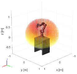
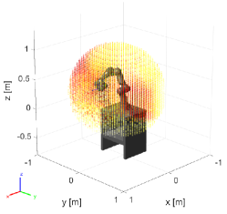
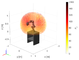
(a)                        (b)                     (c)

Figure 2: Workspace maps based on the index $P_{z}(\mbox{\boldmath$x$}_{i})$ with fixed orientations: Flange Down (a), Flange Horizontal (b) and Flange Up (c).

The force $F_{z,\max}$ is a scalar function of the robot configuration. By considering the inverse kinematic function $\mbox{\boldmath$q$}=\mbox{IK}(\mbox{\boldmath$p$})$ of the manipulator, it can be used as an index for mapping the robot workspace. The pose of the manipulator $\mbox{\boldmath$p$}=[\mbox{\boldmath$x$}^{T},\boldsymbol{\gamma}^{T}]^{T}$ is described by the position $x$ and a minimal representation $\boldsymbol{\gamma}$ of the orientation of the robot end-effector. The 3D space is discretized with a finite number of points $\mbox{\boldmath$x$}_{i}$, and for a given constant orientation $\bar{\boldsymbol{\gamma}}$, each pose $\mbox{\boldmath$p$}_{i}$ is mapped into the corresponding robot configuration $\mbox{\boldmath$q$}_{i}$, and finally to the maximum force that the robot can apply at this point:

$$P_{z}(\mbox{\boldmath$x$}_{i}):\,\,\,\mbox{\boldmath$p$}_{i}=\left[\!\begin{array}[]{c}\mbox{\boldmath$x$}_{i}\\ \bar{\boldsymbol{\gamma}}\end{array}\!\right]\,\,\,\longrightarrow\,\,\,\mbox{\boldmath$q$}_{i}\,\,\,\longrightarrow\,\,\,{F_{z,\max}}_{i}$$

The function $P_{z}(\cdot)$ is called payload index. A four-dimensional dataset $(\mathbf{x}_{i},P_{z}(\mathbf{x}_{i}))$ is obtained. In Fig. 2, a color scale is associated with the payload values to create a 3D representation of the map for a given orientation of the flange. This procedure can be repeated for multiple flange orientations to obtain the desired maps. In the examples depicted in Fig.2, three flange orientations have been considered: Flange Down (a), Flange Horizontal (b), and Flange Up (c). They illustrate the significant variation in payload capability resulting from the different orientations within various regions of the robot’s workspace.

Workspace optimization involves determining the optimal placement of the desired trajectory relative to the cobot’s base reference frame. For a given position $j$, the trajectory, discretized by considering an ordered set of points $\boldsymbol{\varphi}_{k}$, $k=1,\ldots,n$, is ranked based on the minimum value of the payload index, denoted as $\pi_{j}=\min_{k}{P_{z}(\boldsymbol{\varphi}_{k})}$. By iteratively exploring various locations within the robot’s workspace (the trajectory is translated in the $x$ and $y$ directions and rotated around its “center of gravity”) and for different orientations of the end-effector, the optimal configuration is identified as

$$\pi_{\mbox{\small opt}}=\max_{j}\{\pi_{j}\}.$$

The design methodology is summarized in Fig. 3.

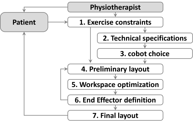
Figure 3: Design methodology for collaborative rehabilitation solutions.

Following the steps in the diagram enables the design of an optimized layout for cobot-assisted rehabilitation solutions, starting from a specific exercise or a set of desired exercises.

Once the layout is defined, and the cobot is installed with the end-effectors in place, ensuring that the system is user-friendly for the therapist and easily customizable becomes crucial. To adjust exercises according to specific requirements or tailor movements to the patient’s anthropometric dimensions, a LbD methodology has been devised. This involves the physiotherapist guiding the cobot’s end-effector via kinesthetic interaction along the desired trajectory.

III Control Architecture for Human-Robot Interaction

A novel control architecture that mixes admittance control and guidance virtual fixtures is developed to constrain the motion of the cobot’s end-effector along a 3D path specified by the therapist without imposing a specific time law. In this way, it is the patient connected to the robot’s end-effector who has to impose the movement along the curve by applying forces with the rehabilitated limb.

\psfrag{m}[c][c][1][0]{ $m,b$}\psfrag{s}[c][c][1][0]{ $s^{\star}$}\psfrag{A}[c][c][1][0]{ $s=0$}\psfrag{B}[c][c][1][0]{ $s=l$}\psfrag{f}[c][c][1][0]{ $\boldsymbol{\varphi}(s)$}\psfrag{F}[c][c][1][0]{ $F_{\parallel}$}\psfrag{H}[c][c][1][0]{ $F_{h}$}\includegraphics[scale={0.55}]{img/ConstrainedDynamics3.eps}

(a)
\psfrag{m}[c][c][1][0]{ $m,b$}\psfrag{s}[c][c][1][0]{ $s^{\star}$}\psfrag{A}[c][c][1][0]{ $s=0$}\psfrag{B}[c][c][1][0]{ $s=l$}\psfrag{f}[c][c][1][0]{ $\boldsymbol{\varphi}(s)$}\psfrag{F}[c][c][1][0]{ $F_{\parallel}$}\psfrag{H}[c][c][1][0]{ $F_{h}$}\psfrag{F}[c][c][1][0]{ ${\color[rgb]{1,0,0}\boldsymbol{F_{h}}}$}\psfrag{X}[c][c][1][0]{ ${\color[rgb]{1,0,0}\boldsymbol{\dot{x}}}$}\psfrag{H}[c][c][1][0]{ Human}\psfrag{R}[c][c][1][0]{ Robot}\psfrag{V}[c][c][1][0]{ \parbox{56.9055pt}{\centering Admittance Guiding Virtual Fixture\@add@centering}}\psfrag{C}[c][c][1][0]{ \parbox{56.9055pt}{\centering Cartesian Impedance Control\@add@centering}}\psfrag{u}[c][c][1][0]{ $\boldsymbol{\hat{F}_{h}}$}\psfrag{d}[c][c][1][0]{ $\mbox{\boldmath$x$}_{d}$}\psfrag{e}[c][c][1][0]{ $\dot{\mbox{\boldmath$x$}}_{d}$}\psfrag{f}[c][c][1][0]{ $\ddot{\mbox{\boldmath$x$}}_{d}$}\psfrag{T}[c][c][1][0]{ $\boldsymbol{\tau}$}\includegraphics[width=433.62pt]{img/Modello_schema_blocchi.eps} (b)

Figure 4: Working principle of the proposed control architecture based on a constrained point-wise mass (a), and related block scheme representation (b).

As mentioned in the introduction, the basic idea, which relies on a virtual proxy [31, 23] affected by the force exchanged with the user, is quite common in haptic and human-robot interaction applications. However, the implementation we propose is novel and presents several advantages, which will be discussed in the following.
Let us assume that the reference path, denoted as $\boldsymbol{x_{d}}$, has been settled by the therapist using a LbD procedure, and is defined by a parametric function:

$$\boldsymbol{x_{d}}=\boldsymbol{\varphi}(u).$$ (4)

Function $\boldsymbol{\varphi}(\cdot)$ represents any curve with a proper degree of continuity, i.e. at least of class $\mathcal{C}^{1}$. In the experiments, we consider cubic B-spline functions, obtained by interpolating the points registered when the user executes the robotic rehabilitation task according to a LbD approach.
In kinesthetic teaching, the independent variable $u$ is typically time (or some related function), ensuring that the trajectory $\mbox{\boldmath$x$}_{d}$ precisely replicates the demonstrated motion. However, since the proposed application aims to enforce a prescribed geometric path without specifying how the path is tracked, an arc-length parameterization should be considered. This can be achieved by composing the function $\boldsymbol{\varphi}(u)$ in (4) with the function $u=u(s)$, which defines how the independent variable $u$ changes with arc length $s$. The function $u(s)$ can be obtained by inverting the function

$$s(u)=\int_{u_{0}}^{u}\left\|\frac{d\boldsymbol{\varphi}(\tau)}{d\tau}\right\|d\tau$$

which can be easily computed numerically during the interpolation procedure of the data points recorded from the demonstrated trajectory [32, 33]. With a slight abuse of notation, we denote $\boldsymbol{\varphi}(s)=\boldsymbol{\varphi}(u(s))$.

As shown in Fig. 4(a), a point-wise mass $m$ is constrained to follow the $\boldsymbol{\varphi}(s)$ and moves subject to the force applied by the user to the robot end-effector. Simultaneously, the cobot needs to accurately track the position of the mass. In Fig. 4(b), a block-scheme representation of the overall control architecture is depicted. The Admittance Guiding Virtual Fixture is obtained by computing the forward dynamics of the virtual mass, considering the measured force $\hat{}\mbox{\boldmath$F$}_{h}$. This approach allows us to obtain the instantaneous value of the reference position, given by

$$\ x_{d}(t)=\boldsymbol{\varphi}(s(t)).$$ (5)

Note that, given $x_{d}(t)$, its derivative can be easily computed analytically as follows:

$$\dot{\mbox{\boldmath$x$}}_{d}(t) = \boldsymbol{\varphi}^{\prime}(s)\dot{s}(t)$$

$$\ddot{\mbox{\boldmath$x$}}_{d}(t) = \boldsymbol{\varphi}^{\prime\prime}(s)\dot{s}^{2}(t)+\boldsymbol{\varphi}^{\prime}(s)\ddot{s}(t)$$

where $\boldsymbol{\varphi}^{\prime}(s)=\frac{d\boldsymbol{\varphi}(s)}{ds}$ and $\boldsymbol{\varphi}^{\prime\prime}(s)=\frac{d^{2}\boldsymbol{\varphi}(s)}{ds^{2}}$. In the following the dynamic behavior of the proxy and the position control of the robot are detailed.
Dynamic equation of the virtual mass
The dynamic model of the point mass $m$ is deduced by applying the standard procedure based on Lagrange equations. With the basic assumption that the mass constrained to the curve $\boldsymbol{\varphi}(s)$ is not affected by gravity, the Lagrangian function equals the kinetic energy

$$\mathcal{L}=\mathcal{K}=\frac{1}{2}m\dot{\mbox{\boldmath$x$}}_{d}^{T}\dot{\mbox{\boldmath$x$}}_{d}=\frac{1}{2}m\dot{s}^{2},$$ (6)

where the fact that, for the arc-length parameterization, $\|\boldsymbol{\varphi}^{\prime}(s)\|=1$ has been exploited. The Lagrange equation for (6) with respect to $s$ yields

$$m\ddot{s}+b\dot{s}=F_{\parallel}$$ (7)

where the $b\dot{s}$ is a non-conservative term taking into account the friction and $F_{\parallel}$ is the component of force $\boldsymbol{\hat{F}}_{h}$ applied by the user to the robot tool (and detected by a force sensor) which is tangent to the curve, i.e.

$$F_{\parallel}=\boldsymbol{\varphi}^{\prime}(s)^{T}\cdot\boldsymbol{\hat{F}}_{h}$$ (8)

where, because of the use of arc-length parameterization, $\boldsymbol{\varphi}^{\prime}(s)$ represents the unit tangent vector to $\boldsymbol{\varphi}(s)$, at a generic point $s$.
The other components of the force $\boldsymbol{\hat{F}}_{h}$, that do not contribute to accelerating the mass, are compensated by the constraints.
Note that if $m\approx 0$ a proportional relationship between the tangent force and the velocity along the curve, which is the most common solution for Admittance-type VF [23], is obtained.
Cartesian impedance control of the robot
Consider the dynamic model of a robot manipulator interacting with a human in (2). The control law

$$\boldsymbol{\tau}=\mathbf{M}(\mathbf{q})\mbox{\boldmath$y$}+\mathbf{C}(\mathbf{q},\dot{\mathbf{q}})\dot{\mathbf{q}}+\mathbf{g}(\mathbf{q})$$ (9)

with the auxiliary input

$$\mbox{\boldmath$y$}=\mathbf{J}^{-1}(\mathbf{q})\left(\ddot{}\mbox{\boldmath$x$}_{d}-\boldsymbol{\dot{J}}(\mbox{\boldmath$q$})\dot{}\mbox{\boldmath$q$}+\mathbf{K}_{D}^{\prime}\dot{\tilde{\mathbf{x}}}+\mathbf{F}_{el}^{\prime}(\tilde{\mathbf{x}})+\mathbf{C_{A}^{\prime}}(\mathbf{q},\dot{\mathbf{q}})\dot{\mathbf{\tilde{\mbox{\boldmath$x$}}}}\right)$$ (10)

leads to the closed loop dynamics:

$$\ddot{\tilde{\mathbf{x}}}+\left(\mathbf{K}_{D}^{\prime}+\mathbf{C_{A}^{\prime}}(\mathbf{q},\dot{\mathbf{q}})\right)\dot{\mathbf{\tilde{\mbox{\boldmath$x$}}}}+\mathbf{F}_{el}^{\prime}(\tilde{\mathbf{x}})=\mathbf{M}_{A}^{-1}(\mathbf{q})\mathbf{F_{h}}$$ (11)

where $\tilde{\mathbf{x}}=\mathbf{x}-\mathbf{x_{d}}$ represents the Cartesian error with respect to the desired pose $\mathbf{x_{d}}$. Finally, assuming:

$$\mathbf{K}_{D}^{\prime} = \mathbf{M}_{A}^{-1}\mathbf{K}_{D}$$ (12)

$$\mathbf{C_{A}^{\prime}}(\mathbf{q},\dot{\mathbf{q}}) = \mathbf{M}_{A}^{-1}\mathbf{C_{A}}(\mathbf{q},\dot{\mathbf{q}})$$ (13)

$$\mathbf{F}_{el}^{\prime}(\tilde{\mathbf{x}}) = \mathbf{M}_{A}^{-1}\mathbf{F}_{el}(\tilde{\mathbf{x}})$$ (14)

the impedance model of the robot in the Cartesian space becomes:

$$\mathbf{M}_{A}(\mathbf{q})\ddot{\tilde{\mathbf{x}}}+\Big{(}\mathbf{K}_{D}+\mathbf{C}_{A}(\mathbf{q},\dot{\mathbf{q}})\Big{)}\dot{\tilde{\mathbf{x}}}+\mathbf{F}_{el}(\tilde{\mathbf{x}})=\mathbf{F}_{h}$$ (15)

The matrices $\mathbf{M}_{A}(\mbox{\boldmath$q$})=\mathbf{J}_{A}^{-T}(\mathbf{q})\mathbf{M}(\mathbf{q})\mathbf{J}_{A}^{-1}(\mathbf{q})$ and $\mathbf{C}_{A}(\mathbf{q},\dot{\mathbf{q}})$ are the robot inertia matrix and the Coriolis and centrifugal matrix in the Cartesian space, respectively. Note that for the matrix $\mathbf{C}_{A}(\mathbf{q},\dot{\mathbf{q}})$ the skew symmetry of $\dot{\mathbf{M}}_{A}(\mbox{\boldmath$q$})-2\mathbf{C}_{A}(\mathbf{q},\dot{\mathbf{q}})$ must hold, i.e. $\mathbf{C}_{A}(\mathbf{q},\dot{\mathbf{q}})=1/2\dot{\mathbf{M}}_{A}(\mbox{\boldmath$q$})$. Matrix $\mathbf{K}_{D}>0$ is the desired damping matrix and, finally, $\mathbf{F}_{el}(\tilde{\mathbf{x}})$ is a generic elastic force, obtained by differentiating a scalar (potential) function $U_{el}(\tilde{\mathbf{x}})\geq 0$, where $U_{el}(\tilde{\mathbf{x}})=0$ if and only if $\tilde{\mathbf{x}}=0$:

$$\mathbf{F}_{el}(\tilde{\mathbf{x}})=\left(\frac{\partial U_{el}(\tilde{\mathbf{x}})}{\partial\tilde{\mathbf{x}}}\right)^{T}.$$ (16)

As highlighted in [34], (15) represents a passive mapping from the external force $\mathbf{F}_{h}$ to the velocity error $\dot{\tilde{\mathbf{x}}}$, ensuring the stability of the system in feedback interconnection with a passive environment.
Finally, note that the inclusion of the acceleration $\ddot{}\mbox{\boldmath$x$}_{d}(t)$ in the control signal (10) justifies the adoption of second-order dynamics in (7) to model the evolution of $s(t)$, that otherwise could lead to infinite values for this variable.

III-A Stability Analysis

As illustrated in Fig. 4(b), the overall control scheme is composed of three subsystems, namely Patient, Admittance Guidance VF and Controlled Robot. Its stability relies on the basic assumption that humans behave in a passive manner, at least when the position of their limbs is kept constant [35, 36, 37]. We assume accordingly that the human operator defines a passive velocity ($\dot{}\mbox{\boldmath$x$}$) to force ($-\mbox{\boldmath$F$}_{h}$) map. Therefore, to assure the stability of the overall system that forms a negative feedback interconnection with the user, it is sufficient to prove that the map from the force applied to the robot $\mbox{\boldmath$F$}_{h}$ and its velocity $\dot{}\mbox{\boldmath$x$}$ is passive as well. This can be done, by considering for the dynamical system composed by (7) and (15), and characterized by the state vector $\xi=[\dot{s},\,\tilde{}\mbox{\boldmath$x$},\dot{\tilde{}\mbox{\boldmath$x$}}]^{T}$, the storage function

$$S_{r}(\xi)=\frac{1}{2}m\dot{s}^{2}+\frac{1}{2}\boldsymbol{\dot{\tilde{x}}}^{T}\mbox{\boldmath$M$}_{A}(\boldsymbol{q})\boldsymbol{\dot{\tilde{x}}}+U_{el}(\tilde{\mbox{\boldmath$x$}}).$$ (17)

The time derivative of (17) yields

$$\dot{S}_{r}(\xi)=m\dot{s}\ddot{s}+\dot{\tilde{\mathbf{x}}}^{T}\mathbf{M}_{A}(\mathbf{q})\ddot{\tilde{\mathbf{x}}}+\frac{1}{2}\dot{\tilde{\mathbf{x}}}^{T}\dot{\mathbf{M}}_{A}(\mathbf{q})\dot{\tilde{\mathbf{x}}}+\frac{\partial U_{el}(\tilde{\mathbf{x}})}{\partial\tilde{\mathbf{x}}}\dot{\tilde{\mathbf{x}}}$$ (18)

which, evaluated along the system trajectories, becomes

$$\dot{S}_{r}(\xi)=-b\dot{s}^{2}+\dot{s}\boldsymbol{\varphi}^{\prime}(s)^{T}\hat{\mbox{\boldmath$F$}}_{h}-\dot{{\tilde{\mbox{\boldmath$x$}}}}^{T}\mbox{\boldmath$K$}_{D}\dot{\tilde{\mbox{\boldmath$x$}}}+\dot{\tilde{\mbox{\boldmath$x$}}}^{T}\boldsymbol{F}_{h}$$ (19)

Finally, by considering that $\boldsymbol{\dot{\mbox{\boldmath$x$}}}_{d}=\boldsymbol{\varphi}^{\prime}(s)\dot{s}$, $\dot{\tilde{\mbox{\boldmath$x$}}}=\dot{\mbox{\boldmath$x$}}-\dot{\mbox{\boldmath$x$}}_{d}$, and that the measured force equals the actual value, i.e. $\hat{}\mbox{\boldmath$F$}_{h}=\mbox{\boldmath$F$}_{h}$, (19) becomes

$$\dot{S}_{r}(\xi)=-b\dot{s}^{2}-\dot{{\tilde{\mbox{\boldmath$x$}}}}^{T}\mbox{\boldmath$K$}_{D}\dot{\tilde{\mbox{\boldmath$x$}}}+\dot{{\mbox{\boldmath$x$}}}^{T}\boldsymbol{F}_{h}.$$ (20)

Being $b>0$ and $\mbox{\boldmath$K$}_{D}>0$,

$$\dot{S}_{r}(\xi)\leq\dot{{\mbox{\boldmath$x$}}}^{T}\boldsymbol{F}_{h}.$$

Thus, the system is passive w.r.t. the pair $\langle\dot{}\mbox{\boldmath$x$},\,\mbox{\boldmath$F$}_{h}\rangle$.

III-B Quasi-static behavior

Once it has been proven that the robotic system connected to the user is stable, it becomes of interest to consider the achievable performance in terms of position error and exchanged forces while the human is interacting with it. Assuming that velocities and accelerations involved in a typical rehabilitation task are very small, we want to analyze the behaviour of the controlled robot, when $\dot{}\mbox{\boldmath$x$}\approx 0$ and $\ddot{}\mbox{\boldmath$x$}\approx 0$, that is close to an equilibrium state. Considering that the user is exerting a constant force $\bar{\mathbf{F}}_{h}$, equations (7) and (15) imply that at equilibrium:

$$F_{\parallel}=\boldsymbol{\varphi}^{\prime}(\bar{s})^{T}\cdot\bar{\boldsymbol{F}}_{h} = 0$$ (21)

$$\mbox{\boldmath$F$}_{el}(\tilde{\mathbf{x}}) = \bar{\boldsymbol{F}}_{h}.$$ (22)

Equation (21) shows that the force applied by the user at the equilibrium must be orthogonal to the tangent vector to the desired curve $\bar{\mathbf{x}}_{d}=\boldsymbol{\varphi}(\bar{s})$, while equation (22) indicates that it must be counteracted by the elastic force acting on the robot, which is caused by the deviation $\bar{\mathbf{x}}$ from $\bar{\mathbf{x}}_{d}$.
From an intuitive user perspective, the system’s displacement, denoted by $\tilde{}\mbox{\boldmath$x$}$, should ideally align with the force causing it, similar to a standard mechanical spring. To achieve this, we can impose a specific structure on the elastic force function, $\mathbf{F}_{el}(\tilde{\mathbf{x}})$, as follows:

$$\mbox{\boldmath$F$}_{el}(\tilde{\mbox{\boldmath$x$}})=f_{el}(\|\tilde{\mbox{\boldmath$x$}}\|)\,\frac{\tilde{}\mbox{\boldmath$x$}}{\|\tilde{\mbox{\boldmath$x$}}\|}$$ (23)

where $f_{el}(\cdot)\geq 0$ is a scalar function, such that $f_{el}(0)=0$. In this way, the elastic force is always directed along $\tilde{\mbox{\boldmath$x$}}$ and its intensity is determined by $f_{el}(\cdot)$. However, the elastic connection plays different roles along the tangent and orthogonal directions to the curve. It needs to ensure minimal tracking error along the curve while still allowing patients to deviate from the planned path without encountering excessive forces. To achieve this, the elastic force has been decomposed into two complementary components:

$$\mbox{\boldmath$F$}_{el}(\tilde{\mbox{\boldmath$x$}})=\mbox{\boldmath$F$}_{el,\parallel}(\tilde{\mbox{\boldmath$x$}}_{\parallel})+\mbox{\boldmath$F$}_{el,\bot}(\tilde{\mbox{\boldmath$x$}}_{\bot})$$ (24)

where

$$\tilde{\mbox{\boldmath$x$}}_{\parallel} = \boldsymbol{\varphi}^{\prime}(\bar{s})\boldsymbol{\varphi}^{\prime}(\bar{s})^{T}\,\tilde{\mbox{\boldmath$x$}}$$

$$\tilde{\mbox{\boldmath$x$}}_{\bot} = \left(\mbox{\boldmath$I$}_{3}-\boldsymbol{\varphi}^{\prime}(\bar{s})\boldsymbol{\varphi}^{\prime}(\bar{s})^{T}\right)\,\tilde{\mbox{\boldmath$x$}}$$

represent the tangent and orthogonal displacements to the curve at point $\boldsymbol{\varphi}(\bar{s})$, respectively. Functions $\mbox{\boldmath$F$}_{el,\parallel}(\cdot)$ and $\mbox{\boldmath$F$}_{el,\bot}(\cdot)$ maintan the structure described in (23). From (24) and (23), the potential function that defines $\mathbf{F}_{el}(\tilde{\mathbf{x}})$ according to (16) can be easily derived as:

$$U_{el}(\tilde{\mbox{\boldmath$x$}})=u_{el,\parallel}(\|\tilde{\mbox{\boldmath$x$}}_{\parallel}\|)+u_{el,\bot}(\|\tilde{\mbox{\boldmath$x$}}_{\bot}\|)$$

where $\displaystyle u_{el,\ast}(z)=\int\,f_{el,\ast}(z)dz$ is the primitive of $f_{el,\ast}(\cdot)$ such that $u_{el,\ast}(0)=0$.
If, for instance, it is assumed $f_{el,\ast}(z)=\kappa\,z$ where $\kappa$ is a positive constant, the constitutive equation of a standard linear spring is obtained, i.e.

$$\mbox{\boldmath$F$}_{el,\ast}(\tilde{\mbox{\boldmath$x$}}_{\ast})=\kappa\,\tilde{\mbox{\boldmath$x$}}_{\ast}.$$ (25)

This expression is used along the tangent direction, where a large value of $\kappa$ helps ensure minimal tracking error. However, due to equations (21) and (22), this component is not perceived by the user when moving slowly along the curve.

A more effective way to define a fixture for rehabilitation applications in the normal plane to the desired path is based on the function:

$$f_{el,\ast}(z)=\displaystyle\chi\frac{\delta^{2}z}{\delta^{2}-z^{2}}\,\,\,\Rightarrow\,\,\,\mbox{\boldmath$F$}_{el,\ast}(\tilde{\mbox{\boldmath$x$}}_{\ast})=\displaystyle\chi\frac{\delta^{2}}{\delta^{2}-\|\tilde{\mbox{\boldmath$x$}}_{\ast}\|^{2}}\tilde{\mbox{\boldmath$x$}}_{\ast}$$ (26)

where $\chi$ and $\delta$ are free parameters that respectively define the stiffness for small deformations ($z\approx 0$) and the maximum allowable displacement, as shown in Fig. 5. When $z$ approaches $\delta$, the magnitude of the elastic force tends to infinity. In this way, the motion of the patient during the exercise is restricted to a maximum distance $\delta$ in the normal direction to the desired geometric path.
Interestingly enough, the potential function derived from (26), i.e.

$$U_{el,\ast}(\tilde{\mbox{\boldmath$x$}}_{\ast})=\frac{\chi\delta^{2}}{2}\log\biggl{(}\frac{\delta^{2}}{\delta^{2}-\|\tilde{\mbox{\boldmath$x$}}_{\ast}\|^{2}}\biggr{)},$$ (27)

has the same form as standard Barrier Lyapunov Functions [38], used for preventing constraint violation in dynamic systems, as they grow to infinity when their argument approaches the given limit $\delta$.

\psfrag{F}[c][c][1][0]{$f_{el}(\|\boldsymbol{\tilde{x}_{\bot}}\|)$ {\small[N]}}\psfrag{x}[c][c][1][0]{$\|\boldsymbol{\tilde{x}_{\bot}}\|$ {\small[mm]}}\psfrag{aaaaaaaaa}[l][l][0.6][0]{$\chi=1$ \small{[N/mm]}}\psfrag{bbbbbb}[l][l][0.6][0]{$\chi=2$ \small{[N/mm]}}\psfrag{cccccc}[l][l][0.6][0]{$\chi=4$ \small{[N/mm]}}\includegraphics[width=346.89731pt]{img/f_el.eps}

Figure 5: Nonlinear elastic function $f_{el}(\|\boldsymbol{\tilde{x}_{\bot}}\|)=\chi\frac{\delta^{2}\|\boldsymbol{\tilde{x}_{\bot}}\|}{\delta^{2}-\|\boldsymbol{\tilde{x}_{\bot}}\|^{2}}$ for different values of parameter $\chi$ ($\delta=5$ [mm]).

\psfrag{f}[c][c][1][0]{ ${\color[rgb]{1,0,0}\mbox{\boldmath$F$}_{h}}$}\psfrag{F}[c][c][1][0]{ ${\color[rgb]{1,0,0}\mbox{\boldmath$F$}_{\bot}}$}\psfrag{P}[c][c][1][0]{ $\boldsymbol{\varphi}(s)$}\psfrag{S}[c][c][1.25][0]{ $\bar{s}$}\psfrag{T}[c][c][1][0]{ ${\color[rgb]{1,0,0}F_{\parallel}}$}\psfrag{p}[c][c][0.8][0]{ $\mbox{\boldmath$F$}_{el}(\tilde{\mathbf{x}})$}\psfrag{d}[c][c][1][0.8]{ $\mbox{\boldmath$K$}_{D}$}\includegraphics[width=303.53267pt]{img/FrankaTrj2.eps}

Figure 6: Equivalent mechanical system of the proposed controller in an equilibrium configuration.

In Fig. 6, the behavior of the overall system is illustrated by means of an equivalent mechanical representation: while the human force $\mathbf{F}_{h}$ affects the robot, only its tangent component moves the mass along the desired path. At equilibrium, when this component is equal to zero, the normal component $F_{\bot}$ causes a deviation from the desired geometric path along the normal direction. The control scheme obtained with the elastic function defined by

$$\mbox{\boldmath$F$}_{el}(\tilde{\mbox{\boldmath$x$}})=\kappa\,\tilde{\mbox{\boldmath$x$}}_{\parallel}\,+\,\chi\frac{\delta^{2}}{\delta^{2}-\|\tilde{\mbox{\boldmath$x$}}_{\bot}\|^{2}}\tilde{\mbox{\boldmath$x$}}_{\bot}$$

is a specific instance of a band-type controller. This type of controller defines the boundaries of a virtual channel, where the motion of the human limb is constrained by forces applied in the normal direction [10, 39]. In the proposed architecture, within the channel, there exists a residual elastic force towards the reference trajectory whose intensity can be freely chosen by adjusting $\chi$.
In this way, the movement of the human limb is not restricted to a specific trajectory [40] or a velocity profile [41, 42], but is determined by the interaction between the user and the robot/virtual mass. The absence of a time constraint in the execution of the exercise makes the duration of the motion a useful parameter for estimating the functional ability of the subjects.

Moreover, the proposed scheme, based on Admittance Guiding Virtual Fixture, offers additional advantages, namely:

• The implementation, based on force-to-position causality, does not require knowledge of the normal direction to the desired reference path [43], whose estimation can be computationally expensive and, in some cases, even impossible since multiple solutions may exist, e.g., when a path has an intersection.

• Help-as-needed mechanisms or, conversely, resisting forces can be easily integrated into the control scheme by adding an appropriate virtual force in Equation (7) governing the mass dynamics.

IV Experimental Results

The proposed methodology, which involves selecting the optimal robot configuration, programming the rehabilitative task through demonstration, and executing it via human-robot interaction, has been tested using a Franka Emika Panda, a collaborative robot with 7 degrees of freedom equipped with an Axia80-M20 force-torque sensor mounted on its terminal flange. It is important to note that the robot is redundant, and as a result, it is necessary to consider its null space dynamics. The resolution of the redundancy problem stemming from the robot’s structure is elaborated in Sec. IV-B.

The goal of the experiments is to simulate a training session in which the user (i.e., the patient) performs a motion that the therapist specifically defines. The objective is to evaluate the impact of control parameters, particularly the stiffness level $\chi$, the radius of the channel $\delta$, and the implementation of additional assisting/opposing mechanisms on the execution of the task. Moreover, a further aspect to be investigated is the user’s perception through the evaluation of physical and psychological aspects. To achieve this, we conducted the following types of tests:

• Simulate a standard execution in various conditions of control parameters.

• Perform a qualitative investigation of user perceptions.

IV-A Path Generation via LbD

In order to define the geometric path for an exercise, the therapist guides the robot’s end-effector, which in this case is a simple handle, within its operational range and the sequence of points, sampled with period $T_{s}$, are recorded. These points are then interpolated with a B-spline curve, i.e. a parametric curve $\boldsymbol{\varphi}(u):[u_{\min},u_{\max}]\rightarrow\mathbb{R}^{3}$ defined as linear combinations of control points $\mbox{\boldmath$p$}_{j}\in\mathbb{R}^{3}$ weighted by B-spline basis functions of degree $p$, $B_{j}^{p}(u)$:

$$\boldsymbol{\varphi}(u)=\sum_{j=0}^{N}\mbox{\boldmath$p$}_{j}B_{j}^{p}(u),~{}~{}~{}~{}~{}~{}~{}u_{\min}\leq u\leq u_{\max}.$$ (28)

The vectorial coefficients $\mbox{\boldmath$p$}_{j},\,j=0,\ldots,\,N$, determine the shape of the curve and are computed by imposing approximation conditions on the samples ${\bf q}_{j}$, $j=0,\ldots,n$ of the recorded trajectory. In particular, to suppress unwanted movements that affect the user’s motion, smoothing B-splines [19] are considered since they minimize the cost function:

$$J:=\sum_{j=0}^{n}w_{j}\|\boldsymbol{\varphi}(u^{\star}_{j})-{\bf q}_{j}\|^{2}+\lambda\int_{u_{\min}}^{u_{\max}}\left\|\frac{d^{2}\boldsymbol{\varphi}(\tau)}{d\tau^{2}}\right\|^{2}d\tau.$$ (29)

Therefore, they represent a trade-off between the squared approximation error with respect to the demonstrated trajectory and the smoothness of the resulting curve. The parameter $\lambda\geq 0$ can be freely chosen to govern this trade-off, while $w_{j}>0$ is a parameter used to selectively weight the contribution of the squared error at a particular point ${\bf q}_{j}$.

The resulting path is depicted in Fig. 7. For the sake of clarity, a planar motion has been defined.

\psfrag{X}[c][c][0.9][0]{ $x$ {\small[m]}}\psfrag{Z}[c][c][0.9][0]{ $z$ {\small[m]}}\includegraphics[width=260.17464pt]{img/path.eps}

Figure 7: B-spline reference path defined via kinesthetic teaching.

It is worth noting that the path exhibits an intersection at a certain point. Consequently, while there is no uncertainty regarding the position along the path, the normal direction at this point is not uniquely defined. This characteristic is particularly advantageous when the virtual constraint is active during the exercise, as it ensures that the patient is consistently returned to the correct point on the path in case of deviation. Consequently, this approach effectively addresses the geometric challenge of maintaining the desired distance between the patient’s actual position and the position defined by the therapist, offering a viable solution in any condition.
As a final note, it is worth highlighting that in these experiments, the orientation of the end-effector has been kept constant, aligned with the axes of the base reference frame. However, despite the mechanism for Human-Robot interaction being solely based on position, being the variable $s$ the arc-lenth along the spatial curve $\boldsymbol{\varphi}$, It is possible to define a function $\boldsymbol{\varphi}_{o}(s)$ that provides a minimal representation of the orientation as a function of progress along the path. This curve can be obtained by interpolating the orientations imposed by the therapist during the demonstration, just like the position.

IV-B Overcoming Redundancy: Strategies for Resolution

The use of a collaborative robot with a redundant kinematic structure is not strictly necessary for the proposed application. However, in a Human-Robot Interaction task, the additional degree of freedom can be profitably exploited to address practical concerns, such as joint limits reaching. For this reason, in addition to the primary control strategy that restricts the motion of the robot’s end-effector along the desired path, as described in Section III, a secondary task has been incorporated into the null space of the end effector task. This is accomplished by adding the additional control input to the control torque in (11):

$$\boldsymbol{{\tau}_{r}}=(\mbox{\boldmath$I$}_{7}-\mbox{\boldmath$J$}^{T}\mbox{\boldmath$J$}^{\dagger^{T}})\boldsymbol{{\tau}_{0}}$$ (30)

where the matrix ${\mbox{\boldmath$J$}}^{\dagger}$ denotes the generalized inverse of Jacobian matrix $J$, as defined by [44]. The matrix $\mbox{\boldmath$I$}_{7}-\mbox{\boldmath$J$}^{\dagger}\mbox{\boldmath$J$}$ is a projection operator that maps the additional arbitrary torques $\boldsymbol{\tau_{0}}$ into the null space of the end effector. It is important to emphasize that the dynamics described by equation (15) only account for the dynamics of the manipulator in the workspace and do not incorporate the dynamics of the null space. For this reason, since the control (30) operates in the null space of the manipulator end-effector, it has been excluded from the passivity analysis in Section III-A.

The torque vector $\tau_{0}$ is then computed as:

$$\boldsymbol{\tau_{0}}=-k_{0}\Bigg{(}\frac{\partial w(\mbox{\boldmath$q$})}{\partial\mbox{\boldmath$q$}}\Bigg{)}^{T}$$ (31)

where $k_{0}$ is a positive constant, and $w(\mbox{\boldmath$q$})$ is is an objective function of the joint variable that must be minimized. In particular, we consider the function:

$$w(\mbox{\boldmath$q$})=\frac{1}{2n}\sum_{i=1}^{n}\Bigg{(}\frac{q_{i}-\bar{q_{i}}}{q_{iM}-q_{im}}\Bigg{)}$$ (32)

where $q_{iM}$ ($q_{im}$) is the maximum (minimum) allowable excursion for the joint variable $q_{i}$, and $\bar{q_{i}}$ is the middle value of the joint range [45]. By minimizing this function, the joint variables are kept as close as possible to their central value and, consequently, as far as possible from their limits.

IV-C Experimental Validation

To evaluate the proposed methodology’s performance, we conducted several tests under various conditions. These tests mimicked a rehabilitation exercise along the predefined path shown in Fig. 7. We recorded relevant metrics, including the forces exchanged during Human-Robot Interaction and the deviation of the patient’s actual position from the reference position.
During the first phase, a healthy user with experience conducted a series of experiments to analyze the impact of various control parameters on the system’s performance. Initially, the focus was on the influence of parameters $\chi\in\{100,\,500,\,2500\}$ [N/m] and $\delta\in\{0.01,\,0.02,\,0.03\}$ [m]. This resulted in the $3\times 3$ different scenarios in Fig. 8. In these tests, the parmeters defining the mass dynamics were fixed at $m=5$ [kg] and $b=15$ [Ns/m], respectively. As $\chi$ increases, users experience a stronger guiding force towards the center of the channel when they deviate from the planned path. This feedback mechanism encourages users to stay centered. In contrast, increasing $\delta$ while keeping $\chi$ constant results in a weaker force, creating a sort of ”wall” effect. Users can move freely within the channel until reaching its boundaries, where they encounter significant resistance. This condition causes them to perceive a subtle guiding force along the reference path, typically leading to less accurate exercise execution. However, the limit set by $\delta$ is never exceeded, as shown in Fig. 8.

$\delta=0.01[m]$

$\delta=0.02[m]$

$\delta=0.03[m]$

\psfrag{X}[c][c][0.8][0]{X [m]}\psfrag{Y}[c][c][0.8][0]{Y [m]}\psfrag{Z}[c][c][0.8][0]{Z [m]}\includegraphics[width=433.62pt]{img/New_img/3D_K100_d001.eps}

$\chi=100[N/m]$

\psfrag{X}[c][c][0.8][0]{X [m]}\psfrag{Y}[c][c][0.8][0]{Y [m]}\psfrag{Z}[c][c][0.8][0]{Z [m]}\includegraphics[width=433.62pt]{img/New_img/3D_K100_d002.eps}

\psfrag{X}[c][c][0.8][0]{X [m]}\psfrag{Y}[c][c][0.8][0]{Y [m]}\psfrag{Z}[c][c][0.8][0]{Z [m]}\includegraphics[width=433.62pt]{img/New_img/3D_K100_d003.eps}

\psfrag{X}[c][c][0.8][0]{X [m]}\psfrag{Y}[c][c][0.8][0]{Y [m]}\psfrag{Z}[c][c][0.8][0]{Z [m]}\includegraphics[width=433.62pt]{img/New_img/3D_K500_d001.eps}

$\chi=500[N/m]$

\psfrag{X}[c][c][0.8][0]{X [m]}\psfrag{Y}[c][c][0.8][0]{Y [m]}\psfrag{Z}[c][c][0.8][0]{Z [m]}\includegraphics[width=433.62pt]{img/New_img/3D_K500_d002.eps}

\psfrag{X}[c][c][0.8][0]{X [m]}\psfrag{Y}[c][c][0.8][0]{Y [m]}\psfrag{Z}[c][c][0.8][0]{Z [m]}\includegraphics[width=433.62pt]{img/New_img/3D_K500_d003.eps}

\psfrag{X}[c][c][0.8][0]{X [m]}\psfrag{Y}[c][c][0.8][0]{Y [m]}\psfrag{Z}[c][c][0.8][0]{Z [m]}\includegraphics[width=433.62pt]{img/New_img/3D_K2500_d001.eps}

$\chi=2500[N/m]$

\psfrag{X}[c][c][0.8][0]{X [m]}\psfrag{Y}[c][c][0.8][0]{Y [m]}\psfrag{Z}[c][c][0.8][0]{Z [m]}\includegraphics[width=433.62pt]{img/New_img/3D_K2500_d002.eps}

\psfrag{X}[c][c][0.8][0]{X [m]}\psfrag{Y}[c][c][0.8][0]{Y [m]}\psfrag{Z}[c][c][0.8][0]{Z [m]}\includegraphics[width=433.62pt]{img/New_img/3D_K2500_d003.eps}

Figure 8: Executions of the rehabilitation task defined in Fig. 7 recorded under different values for $\chi$ and $\delta$.

The qualitative observations regarding the influence of control parameters are corroborated by the numerical evaluation of the tests. To ensure statistically significant results, each experiment was repeated ten times. The results are then gathered in a single boxplot.

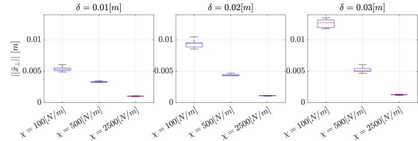
Figure 9: Deviation with respect to the reference path in the orthogonal direction, obtained in the expriments shown in Fig. 8 for different values of parameters $\chi$ and $\delta$.

Figure 9 shows the magnitude of the deviation with respect to the reference path in the orthogonal direction, denoted by $\|\tilde{\mbox{\boldmath$x$}}_{\bot}\|$, experienced by the user in the tests performed for each pair of parameters ($\chi$,$\delta$). It is evident that parameter $\chi$ strongly influences the deviation from the path. As $\chi$ increases, the precision of the execution improves. In contrast, $\delta$ primarily ensures compliance with the maximum allowed displacement, but, for high value of $\chi$, it has no significant effect on the average deviation.
Analyzing the normal forces exchanged between the robot and the user to keep them along the desired path, which are reported in norm in Fig. 10, it is found that these remain practically constant as the parameters vary: in particular, the parameter $\delta$ seems to have no influence, while the parameter $\chi$ tends to slightly increase the average value of the forces.

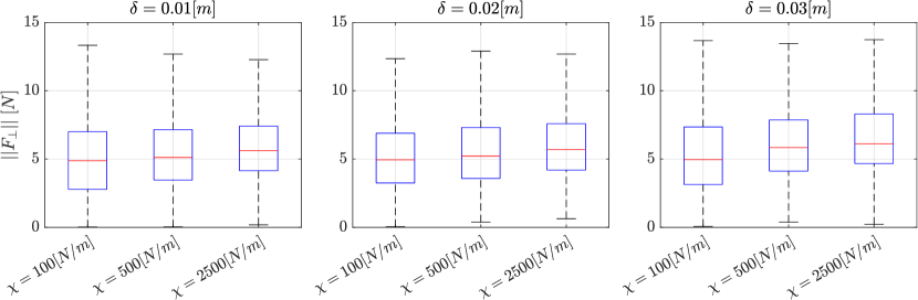
Figure 10: Magnitude of the forces exchanged in the experiments shown in Fig. 8 for different values of parameters $\chi$ and $\delta$.

If we only consider the peak value of the force for each experiment, shown in Fig. 11, the situation changes dramatically. In this case, small values of $\chi$ tend to produce high peak forces. This can be explained by the fact that small values of $\chi$ leave the user with very little guidance, essentially free to move around the desired path. Only when the user approaches the maximum allowed distance does the force suddenly increase, resulting in high peak forces. This phenomenon is particularly evident for the smallest value of $\delta$, where the user tends to bounce between the walls of the virtual tube. Based on the analysis of these numerical results, we can conclude that high values of $\chi$ are desirable. The level of $\delta$ is simply related to the desired precision required by the task and has minimal impact on the exchanged forces.

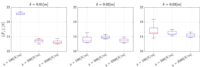
Figure 11: Magnitude of the peak forces exchanged in the experiments shown in Fig. 8 for different values of parameters $\chi$ and $\delta$.

To complete our analysis of the effect of the parameters on control performance and interaction between the robot and user, we also considered $m$ and $b$, which define the dynamics of the virtual mass. We found a correlation between these parameters and the tangential component of the forces exerted by the user, while $\chi$ and $\delta$ have a negligible impact on them.

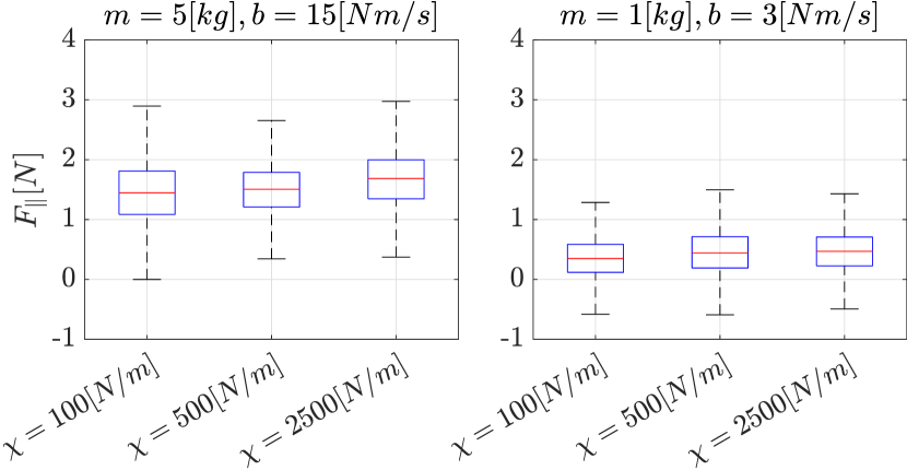
Figure 12: Tangential forces exerted by the user with different values of $m$ and $b$ ($\delta=0.03\;\text{m}$).

As illustrated in Fig. 12, reducing the values to $m=1$ [kg] and $b=3$ [Ns/m] substantially decreases the force component applied by the user, compared to the previously examined scenario. This results in an overall reduction in the physical effort required for task execution. Additionally, besides modifying the parameters $m$ and $b$, the dynamics of the virtual mass in (7) can be tailored to the specific needs of the patient by introducing a virtual force that can be easily adjusted to either assist or hinder the execution of the task.

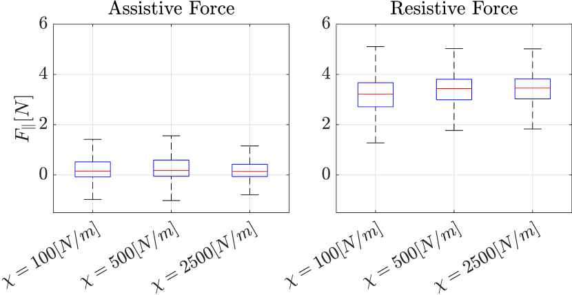
Figure 13: Tangential forces exerted by the user with the application of $1$ N assistive or resistive force.

In Fig. 13, the effects of applying a $\pm 1$ N virtual force are shown. Positive forces are considered assistive, while negative forces are considered resistive. Compared to the standard case in Fig. 12 (left), applying a virtual force modifies the tangetial force required by the user to complete the task by the same amount. While more complex assistive mechanisms can certainly be implemented, this serves as a proof of concept. It demonstrates the benefit of an architecture based on a virtual mass that decouples the dynamics along the desired path from the dynamics in the orthogonal directions, which ideally should be zero.
Recognizing that quality performance is influenced by user behaviour, the second phase of the validation procedure focused on evaluating users’ perceptions during task execution in relation to their interaction with the robot. To explore this relationship, we recruited 10 healthy participants, all of whom provided informed consent prior to participation. The cohort comprised 7 males and 3 females, aged 24 to 65 years with a mean age of 32 years. Importantly, none of the participants had prior experience with robots.
Subjective data were collected through a concise questionnaire. Participants rated their agreement with statements about the controlled system’s performance on a 6-point scale (1 being low, 6 being high). The questions presented to the participants were adapted from the nasa-tlx (task load index), proposed in [46], focusing on Physical Demand, Performance, Effort, and Frustration in task accomplishment. The same questionnaire was administered to users under six different conditions, that represent a subset of the test reported in Fig. 8. Starting from the initial condition $\chi=100$ [N/m] and $\delta=0.01$ [m], first the stiffness $\chi$ is increased and then the radius $\delta$ of the tube is augmented. The aggregated results are reported in Fig. 14.

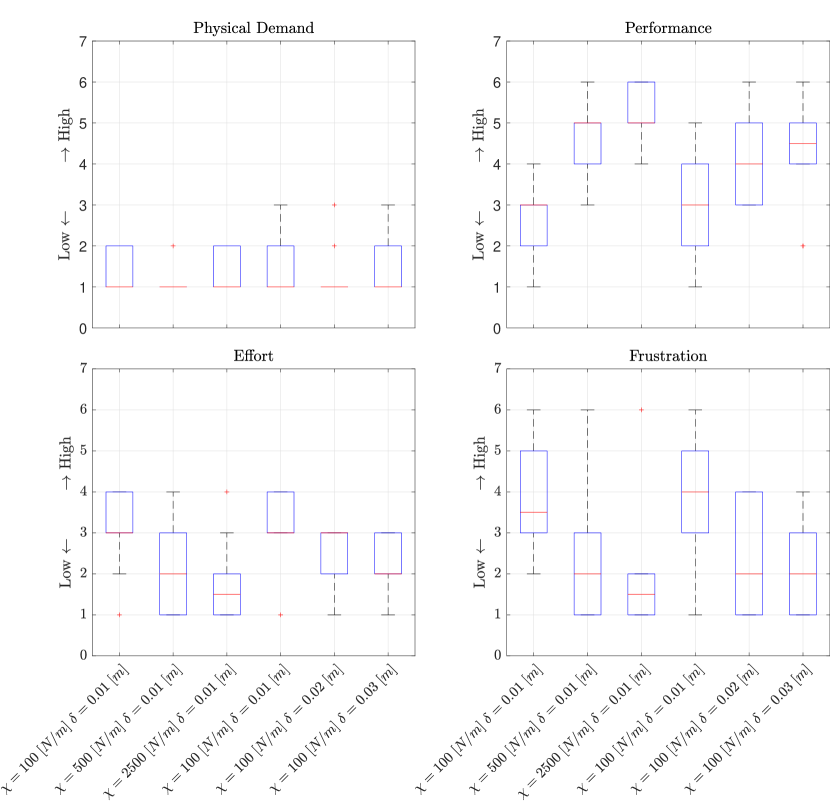
Figure 14: Users’ opinions about Physical Demand, Performance, Effort, and Frustration related to some of the tests are reported in Fig. 8.

The combination of parameters defining the stiffness function (Eq. 26) significantly impacts user perception. Specifically, increasing both $\chi$ and $\delta$ leads to a perceived improvement in performance quality.

• Higher stiffness (increased $\chi$) enhances perceived performance quality. This is because the steeper slope of the stiffness function near the virtual channel’s center reduces execution errors, making users feel more efficient in following the path. Higher values of $\chi$ also reduce the perception of effort. The stronger guidance towards the reference path decreases the effort users feel they need to exert.

• An enlarged virtual channel (increased $\delta$) also improves perceived performance and simplifies task execution. Users experience greater freedom in task execution without feeling like they’re deviating from the intended path. This reduces frustration as users have more space to maneuver within the channel boundaries (especially with higher $\chi$ values).

In each reported condition, physical demand remains very low, making the solution equally suitable for users of all genders.

V Conclusions

This paper presents a layout optimization method and a novel control architecture for collaborative robots applied to upper limb rehabilitation. The system offers therapist-friendly programmability through programming by demonstration (PbD) and incorporates an admittance-type Virtual Fixture control. This control strategy allows the robot to act as a supportive guide for the patient’s movements.

The introduction of assistive and opposing mechanisms within the control architecture allows for tailored resistance or support during task execution. This adaptability is crucial in adjusting the complexity of exercises based on the patient’s needs, potentially enhancing the rehabilitation process.

Experimental validation demonstrated the efficiency and robustness of our solution under various conditions, highlighting the potential benefits for both therapists and patients. The user studies involving healthy participants provided insights into the subjective experience and perceived performance of the control system. Results indicate that appropriate tuning of control parameters significantly improves user interaction and task execution accuracy, confirming the practical applicability of the proposed system in real-world rehabilitation scenarios.

Future work will focus on methods for further enhancing the usability and effectiveness of the collaborative robotic system in tailoring rehabilitation programs to individual patient needs. In particular, the use of EMG signals will be analyzed to determine the optimal level of assistance and evaluate the patient’s state of recovery.

Dario Onfiani received his B.Sc. and M.Sc. degrees in Mechanical Engineering from the University of Modena and Reggio Emilia, Italy, in 2019 and 2022, respectively. He is currently pursuing a Ph.D. degree in Information and Communication Technologies at the same university. His research interests include collaborative robotics, human-robot interaction, and the development of assistive robotic systems for rehabilitation.

Marco Caramaschi received his B.Sc. and M.Sc. degrees in Mechanical Engineering from the University of Modena and Reggio Emilia, Italy, in 2019 and 2022, respectively. He worked on the development of assistive robotic systems for rehabilitation along his research fellowship at Department of Engineering “Enzo Ferrari” of the University of Modena and Reggio Emilia.

Luigi Biagiotti (Member, IEEE) received the Ph.D. degree in automation engineering from the University of Bologna, Italy, in 2003. He is currently an Associate Professor with the Department of Engineering “Enzo Ferrari” of the University of Modena and Reggio Emilia. He is author or coauthor of more than 50 scientific papers presented at conferences or published in journals, and two books on motion planning and automatic control. His research interests include modelling and control of physical systems, trajectory planning and optimization, control of robotic systems, human-robot interaction.

Fabio Pini received the Ph.D. degree in simulation methods and mechanical design from the University of Modena and Reggio Emilia, Italy, in 2008. At the same university, he is currently a Tenure track Professor at the Department of Engineering “Enzo Ferrari”. He is author or coauthor of more than 40 scientific papers. His research interests include the definition of Computer Aided Design approaches for Product and Process Design, specifically oriented to the Development of Collaborative and Industrial robotics solutions and devices.

References

- [1] R. Gassert and V. Dietz, “Rehabilitation robots for the treatment of sensorimotor deficits: a neurophysiological perspective,” Journal of neuroengineering and rehabilitation, 2018.
- [2] T. Nef, M. Guidali, and R. Riener, “Armin iii–arm therapy exoskeleton with an ergonomic shoulder actuation,” Applied Bionics and Biomechanics, 2009.
- [3] T. G. Sugar, J. He, E. J. Koeneman, J. B. Koeneman, R. Herman, H. Huang, R. S. Schultz, D. Herring, J. Wanberg, S. Balasubramanian et al., “Design and control of rupert: a device for robotic upper extremity repetitive therapy,” IEEE transactions on neural systems and rehabilitation engineering, 2007.
- [4] S. Crea, M. Cempini, M. Moise, A. Baldoni, E. Trigili, D. Marconi, M. Cortese, F. Giovacchini, F. Posteraro, and N. Vitiello, “A novel shoulder-elbow exoskeleton with series elastic actuators,” in 2016 6th IEEE International Conference on Biomedical Robotics and Biomechatronics (BioRob). IEEE, 2016.
- [5] M. Caramaschi, D. Onfiani, F. Pini, L. Biagiotti, and F. Leali, “Workspace placement of motion trajectories by manipulability index for optimal design of cobot assisted rehabilitation solutions,” Computer-Aided Design and Applications, pp. 1–12, 2022.
- [6] H. Krebs, , and B. Volpe, “Rehabilitation robotics,” Handbook of clinical neurology, 2013.
- [7] R. Loureiro, F. Amirabdollahian, M. Topping, B. Driessen, and W. Harwin, “Upper limb robot mediated stroke therapy—gentle/s approach,” Autonomous Robots, 2003.
- [8] A. Toth, D. Nyitrai, M. Jurak, I. Merksz, G. Fazekas, and Z. Denes, “Safe robot therapy: Adaptation and usability test of a three-position enabling device for use in robot mediated physical therapy of stroke,” in 2009 IEEE International Conference on Rehabilitation Robotics. IEEE, 2009.
- [9] A. Bertomeu-Motos, A. Blanco, F. J. Badesa, J. A. Barios, L. Zollo, and N. Garcia-Aracil, “Human arm joints reconstruction algorithm in rehabilitation therapies assisted by end-effector robotic devices,” Journal of neuroengineering and rehabilitation, 2018.
- [10] L. Zhang, S. Guo, and Q. Sun, “Development and assist-as-needed control of an end-effector upper limb rehabilitation robot,” Applied Sciences, 2020.
- [11] J. Mehrholz, A. Hädrich, T. Platz, J. Kugler, and M. Pohl, “Electromechanical and robot-assisted arm training for improving generic activities of daily living, arm function, and arm muscle strength after stroke,” Cochrane database of systematic reviews, 2012.
- [12] P. Maciejasz, J. Eschweiler, K. Gerlach-Hahn, A. Jansen-Troy, and S. Leonhardt, “A survey on robotic devices for upper limb rehabilitation,” Journal of NeuroEngineering and Rehabilitation, 2014.
- [13] Z. Qian and Z. Bi, “Recent development of rehabilitation robots,” Advances in Mechanical Engineering, 2015.
- [14] F. Ficuciello, A. Romano, L. Villani, and B. Siciliano, “Cartesian impedance control of redundant manipulators for human-robot co-manipulation,” in IEEE/RSJ International Conference on Intelligent Robots and Systems, 2014.
- [15] A. Q. Keemink, H. van der Kooij, and A. H. Stienen, “Admittance control for physical human–robot interaction,” The International Journal of Robotics Research, 2018.
- [16] N. Hogan, “Impedance control: An approach to manipulation: Part ii—implementation,” Journal of Dynamic Systems, Measurement, and Control, 1985.
- [17] C. Lauretti, F. Cordella, E. Guglielmelli, and L. Zollo, “Learning by demonstration for planning activities of daily living in rehabilitation and assistive robotics,” IEEE Robotics and Automation Letters, 2017.
- [18] J. Aleotti and S. Caselli, “Robust trajectory learning and approximation for robot programming by demonstration,” Robotics and Autonomous Systems, 2006.
- [19] L. Biagiotti and C. Melchiorri, Trajectory Planning for Automatic Machines and Robots, 1st ed. Heidelberg, Germany: Springer, 2008.
- [20] A. J. Ijspeert, J. Nakanishi, H. Hoffmann, P. Pastor, and S. Schaal, “Dynamical movement primitives: learning attractor models for motor behaviors,” Neural computation, 2013.
- [21] H. J. Asl, M. Yamashita, T. Narikiyo, and M. Kawanishi, “Field-based assist-as-needed control schemes for rehabilitation robots,” IEEE/ASME Transactions on Mechatronics, 2020.
- [22] C. Tamantini, F. Cordella, C. Lauretti, F. S. di Luzio, M. Bravi, F. Bressi, F. Draicchio, S. Sterzi, and L. Zollo, “Patient-tailored adaptive control for robot-aided orthopaedic rehabilitation,” in International Conference on Robotics and Automation (ICRA). IEEE, 2022.
- [23] J. J. Abbott, P. Marayong, and A. M. Okamura, “Haptic virtual fixtures for robot-assisted manipulation,” in Robotics Research, S. Thrun, R. Brooks, and H. Durrant-Whyte, Eds. Berlin, Heidelberg: Springer Berlin Heidelberg, 2007, pp. 49–64.
- [24] S. A. Bowyer, B. L. Davies, and F. Rodriguez y Baena, “Active constraints/virtual fixtures: A survey,” IEEE Transactions on Robotics, vol. 30, no. 1, pp. 138–157, 2014.
- [25] M. Saveriano, F. J. Abu-Dakka, A. Kramberger, and L. Peternel, “Dynamic movement primitives in robotics: A tutorial survey,” arXiv preprint arXiv:2102.03861, 2021.
- [26] Z. Pezzementi, A. M. Okamura, and G. D. Hager, “Dynamic guidance with pseudoadmittance virtual fixtures,” in Proceedings 2007 IEEE International Conference on Robotics and Automation, 2007, pp. 1761–1767.
- [27] M. Selvaggio, G. A. Fontanelli, F. Ficuciello, L. Villani, and B. Siciliano, “Passive virtual fixtures adaptation in minimally invasive robotic surgery,” IEEE Robotics and Automation Letters, vol. 3, no. 4, pp. 3129–3136, 2018.
- [28] D. Papageorgiou, T. Kastritsi, Z. Doulgeri, and G. A. Rovithakis, “A passive phri controller for assisting the user in partially known tasks,” IEEE Transactions on Robotics, vol. 36, no. 3, pp. 802–815, 2020.
- [29] N. Diolaiti, G. Niemeyer, F. Barbagli, and J. Salisbury, “Stability of haptic rendering: Discretization, quantization, time delay, and coulomb effects,” IEEE Transactions on Robotics, vol. 22, no. 2, pp. 256–268, 2006.
- [30] L. Zhang, S. Guo, and Q. Sun, “An assist-as-needed controller for passive, assistant, active, and resistive robot-aided rehabilitation training of the upper extremity,” Applied Sciences, vol. 11, no. 1, 2021. [Online]. Available: https://www.mdpi.com/2076-3417/11/1/340
- [31] C. Zilles and J. Salisbury, “A constraint-based god-object method for haptic display,” in Proceedings 1995 IEEE/RSJ International Conference on Intelligent Robots and Systems. Human Robot Interaction and Cooperative Robots, vol. 3, 1995, pp. 146–151 vol.3.
- [32] T. Gašpar, B. Nemec, J. Morimoto, and A. Ude, “Skill learning and action recognition by arc-length dynamic movement primitives,” Robotics and Autonomous Systems, vol. 100, pp. 225–235, 2018. [Online]. Available: https://www.sciencedirect.com/science/article/pii/S0921889017302695
- [33] D. Onfiani, M. Caramaschi, L. Biagiotti, and F. Pini, “Path-constrained admittance control of human-robot interaction for upper limb rehabilitation,” in Social Robotics, F. Cavallo, J.-J. Cabibihan, L. Fiorini, A. Sorrentino, H. He, X. Liu, Y. Matsumoto, and S. S. Ge, Eds. Cham: Springer Nature Switzerland, 2022, pp. 143–153.
- [34] A. Albu-Schaffer, C. Ott, U. Frese, and G. Hirzinger, “Cartesian impedance control of redundant robots: recent results with the dlr-light-weight-arms,” in 2003 IEEE International Conference on Robotics and Automation (Cat. No.03CH37422), vol. 3, 2003, pp. 3704–3709 vol.3.
- [35] M. Dyck, A. Jazayeri, and M. Tavakoli, “Is the human operator in a teleoperation system passive?” in 2013 World Haptics Conference (WHC), 2013, pp. 683–688.
- [36] R. Anderson and M. Spong, “Asymptotic stability for force reflecting teleoperators with time delays.” IEEE, 2023.
- [37] S. Haykin, Active Network Theory, ser. Addison-Wesley series in electrical engineering. Addison-Wesley Publishing Company, 1970. [Online]. Available: https://books.google.it/books?id=8DqzAAAAIAAJ
- [38] K. P. Tee, S. S. Ge, and E. H. Tay, “Barrier lyapunov functions for the control of output-constrained nonlinear systems,” 2009.
- [39] C.-H. Lin, Y.-Y. Su, Y.-H. Lai, and C.-C. Lan, “A spatial-motion assist-as-needed controller for the passive, active, and resistive robot-aided rehabilitation of the wrist,” IEEE Access, 2020.
- [40] J. Zhang and C. C. Cheah, “Passivity and stability of human–robot interaction control for upper-limb rehabilitation robots,” IEEE Transactions on Robotics, 2015.
- [41] H. J. Asl, T. Narikiyo, and M. Kawanishi, “An assist-as-needed velocity field control scheme for rehabilitation robots,” in 2018 IEEE/RSJ International Conference on Intelligent Robots and Systems (IROS). IEEE, 2018.
- [42] M. Najafi, C. Rossa, K. Adams, and M. Tavakoli, “Using potential field function with a velocity field controller to learn and reproduce the therapist’s assistance in robot-assisted rehabilitation,” IEEE/ASME Transactions on Mechatronics, 2020.
- [43] H. R. Z. L. Q. W. D. Wu, “Guidance priority adaptation in human-robot shared control,” in 2022 IEEE International Conference on Mechatronics and Automation (ICMA) —. IEEE, 2022.
- [44] O. Khatib, “A unified approach for motion and force control of robot manipulators: The operational space formulation.” IEEE, 1987.
- [45] B. Siciliano, L. Sciavicco, L. Villani, and G. Oriolo, Robotics: Modelling, Planning and Control, 1st ed. Springer Publishing Company, Incorporated, 2008.
- [46] S. G. Hart and L. E. Staveland, “Development of nasa-tlx (task load index): Results of empirical and theoretical research,” in Advances in psychology. Elsevier, 1988, vol. 52, pp. 139–183.