Casimir-Lifshitz force with graphene: theory versus experiment, role of spatial non-locality and of losses

Abstract

We calculate the Casimir-Lifshitz force (CLF) between a metallic sphere and a graphene-coated SiO₂ plane and compare our finding with the experiment and theory by M. Liu et al., PRL 126, 206802 (2021), where a non-local and lossless model for the graphene conductivity (GC) has been used and shown to be compatible with the experimental results. Recently, that conductivity model has been shown to be not correctly regularized [arXiv:2403.02279], to predict nonphysical results in the non-local regime, and being correct only in its local limit, where its expression is identical to the local Kubo conductivity model (once also losses are introduced). To compare the experimental results with the correctly regularized Kubo theory and to clarify the effective role played by the graphene non-locality and losses in that experiment, we calculated the CLF using three different models for the GC: the correct general non-local Kubo model, the local Kubo model, and the non-regularized and lossless model used by M. Liu et al.. For the parameters of the experiment, the predictions for the Casimir-Lifshitz force using the three models are practically identical, implying that, for the experiment, both non-local and lossy effects in the GC are negligible. This explains why the GC model used in M. Liu et al. provides results in agreement with the experiment. We find that the experiment cannot distinguish between the Drude and Plasma prescriptions. Our findings are relevant for present and future comparisons with experimental measurement of the Casimir-Lifshitz force involving graphene structures. Indeed, we show that an extremely simple local Kubo model, explicitly depending on Dirac mass, chemical potential, losses and temperature, is largely enough for a totally comprehensive comparison with typical experimental configurations.

I Introduction

The Casimir-Lifshitz force (CLF) is an ubiquitous dispersion interaction acting between polarizable objects [1]. Originated by the quantum and thermal fluctuations of the electromagnetic field, it strongly depends on both the geometry and the dielectric properties of the involved bodies. In recent years, with the arrival and extended investigation of 2D materials in different contexts, particular attention has been devoted to the CLF in graphene-based systems[2, 3, 4, 5, 6, 7, 8, 9, 10, 11, 12]. Remarkably, it has been predicted that the CLF between two parallel graphene sheets has an extraordinary high thermal effect already at very short separation [4]. Recently, M. Liu et al. [13] measured the CLF gradient between a metallic sphere and a planar SiO₂ substrate coated with graphene at room temperature (see the scheme in Fig. 1) and compared their results with theory predictions using the standard Lifshitz theory.

A crucial ingredient of the Lifshitz theory is the knowledge of the graphene conductivity (as far as of the dielectric permittivity of all involved materials). Recently, it has been shown that the graphene conductivity model used in the theory analysis in M. Liu et al. [13] is not correct in general [14]. It is then interesting (i) to compare the experimental results with a theory using a correct conductivity model, and (ii) to explain why the theory used in [13] showed a good agreement with the experiment despite the use of a not-correct expression for the graphene conductivity.

To answer these questions, in this article we compare the experiment [13] with the CLF gradient theory predictions obtained by using three different models for the electric conductivity of graphene: (i) the general non-local Kubo (K) formula, derived from the microscopic Ohm law $J_{i}=\sigma_{ij}E^{j}$, the (ii) local limit (L) of the Kubo formula (which, in the zero mass-gap limit reduces to the known Falkovsky model [15]), and (iii) the non-regularized (NR) model derived from the direct relation $J_{i}=\Pi_{ij}A^{j}$ and used in [13].

It is worth stressing that these different conductivity models have been recently investigated in [14]. In particular it has been shown that the NR model not only does not include losses, but that independently on that, it predicts the appearance of a non-physical intrinsic plasma divergent behavior implying a permanent electric current in absence of electric field at room temperature for the transverse polarization coming from the interband conductivity term. The origin of the flows in the NR conductivity has been discussed in detail and the way how to correct it has been provided, showing that once corrected it becomes identical to the general Kubo conductivity.

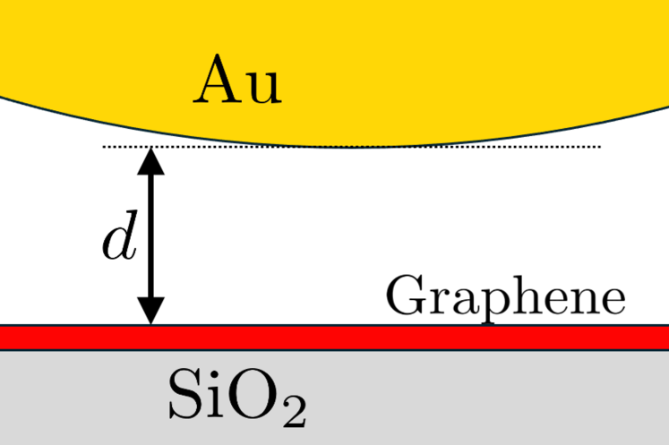
Figure 1: Scheme of the systems, as in the experiment [13]. An SiO₂ plate covered with a single sheet of graphene placed at a distance $d$ of a gold covered sphere of radius $R$.

In addition, our comparative study will elucidate the real role payed by graphene losses and by non-locality in this experiment, showing that both effects are completely negligible for this given experiment, and that the simple local conductivity model is largely enough. We will also investigate the sensitivity of the CLF gradient to the use of a Plasma or a Drude model for the involved metallic materials (gold and graphene) showing that a possible distinction between these two models cannot be explored with this experiment.

The article is organized as follows. In Sect. II and Sect. III we review the Lifshitz formula for calculating the CLF and Fresnel reflection matrices to be used. In Sect. IV, we review the three models for the electric conductivity of graphene we will compare. In Sect. V and Sect. VI, we review the experiment published in [13], check the Drude and Plasma prescriptions, the effect of losses and of non-locality. We finish with the conclusions in Sect. VII.

II Casimir-Lifshitz force

For the geometric configuration of the experiment [13] (see scheme in Fig. 1), the spatial gradient of the CLF $G(d)=\partial_{d}F(d)$ between a gold covered sphere of radius $R$ and a graphene covered SiO₂ plate separated by a distance $d$ can be safely expressed within the Proximity Force Approximation [16] ($d/R<0.012$):

$$G(d)=2k_{B}TR{\displaystyle\sum_{n=0}^{\infty}}^{\prime}\displaystyle\int_{0}^{\infty}\mathrm{d}k_{\parallel}\kappa_{z}k_{\parallel}\text{Tr}\left(\mathbb{N}_{12}\left(\mathbbm{1}-\mathbb{N}_{12}\right)^{-1}\right).$$ (1)

Here $\mathbb{N}_{12}=\mathbb{R}_{1}\mathbb{R}_{2}e^{-2d\kappa_{z}}$, $\mathbb{R}_{\alpha}=\mathbb{R}_{\alpha}(\kappa_{n},{k}_{\parallel})$ is the Fresnel reflection matrix of the $\alpha$-th body, $\kappa_{z}=\sqrt{\kappa_{n}^{2}+{k}_{\parallel}^{2}}$, with $\kappa_{n}=\xi_{n}/c=\frac{2\pi}{\beta\hbar c}n$, $\xi_{n}$ are the Matsubara frequencies, $\beta=(k_{B}T)^{-1}$, and ${k}_{\parallel}$ is the component of the EM wavevector parallel to the surface of the plate. The prime symbol indicates that the $n=0$ term has a $1/2$ weight.

In the following we will also use two limits of Eq. (1), and in particular the zero temperature (T=0) limit:

$$G_{0}(d)=\frac{\hbar cR}{\pi}\!\!\int_{0}^{\infty}\!\!\!\!\!\mathrm{d}\kappa\displaystyle\int_{0}^{\infty}\mathrm{d}k_{\parallel}\kappa_{z}k_{\parallel}\text{Tr}\left(\mathbb{N}_{12}\left(\mathbbm{1}-\mathbb{N}_{12}\right)^{-1}\right),$$ (2)

where $\kappa_{z}=\sqrt{\kappa^{2}+k_{\parallel}^{2}}$, and the high temperature/large distance classical limit, corresponding to the $n=0$ Matsubara term in (1):

$$G_{\rm{cl}}(d)=k_{B}TR\displaystyle\int_{0}^{\infty}\mathrm{d}k_{\parallel}k_{\parallel}^{2}\text{Tr}\left(\mathbb{N}_{12}\left(\mathbbm{1}-\mathbb{N}_{12}\right)^{-1}\right).$$ (3)

III Fresnel Reflection matrices

In this section we provide the expression for the Fresnel reflection matrices $\mathbb{R}_{1}$ and $\mathbb{R}_{2}$, corresponding to an SiO₂ plate coated with graphene and to a gold plate, respectively. These well be then used for the calculation of the CLF gradient $G(d)$.

III.1 SiO₂ plate coated with graphene

In general, the Fresnel matrix coefficients for a planar structure can be decomposed in four blocks:

$$\mathbb{R} = \left(\begin{array}[]{cc}R_{\rm{ss}}&R_{\rm{sp}}\\ R_{\rm{ps}}&R_{\rm{pp}}\end{array}\right).$$ (6)

We consider here the particular case of a structure made by an infinite half space having relative dielectric susceptibility $\epsilon_{1}(\kappa)$ (in this case $\epsilon_{1}(\kappa)$ is the SiO₂ dielectric function) and relative diamagnetic susceptibility $\mu_{1}=1$, coated with graphene sheet having longitudinal and transversal conductivity given by $\sigma_{L}(\kappa,k_{\parallel})$ and $\sigma_{T}(\kappa,k_{\parallel})$, respectively (in this case, we consider that the Hall conductivity is zero $\sigma_{H}(\kappa,k_{\parallel})=0$ because in our case there is no induced time reversal symmetry breaking). Here we consider the conductivity and the dielectric functions along the imaginary frequency axis $\omega=\mathrm{i}\xi=\mathrm{i}c\kappa$. The corresponding terms of the reflection matrix, for imaginary frequencies, are [2, 17, 13]

$$R_{\rm{ss}}^{\rm{Gr}} \equiv R_{TE}^{\rm{Gr}}= \dfrac{\kappa_{z}-\kappa_{1,z}-2\kappa\bar{\sigma}_{T}}{\kappa_{z}+\kappa_{1,z}+2\kappa\bar{\sigma}_{T}},$$ (7)

$$R_{\rm{pp}}^{\rm{Gr}} \equiv R_{TM}^{\rm{Gr}}= \dfrac{\epsilon_{1}\kappa_{z}-\kappa_{1,z}+2\frac{\kappa_{z}\kappa_{1,z}}{\kappa}\bar{\sigma}_{L}}{\epsilon_{1}\kappa_{z}+\kappa_{1,z}+2\frac{\kappa_{z}\kappa_{1,z}}{\kappa}\bar{\sigma}_{L}},$$ (8)

and $R_{\rm{sp}}^{\rm{Gr}}=R_{\rm{ps}}^{\rm{Gr}}=0$. Here $\bar{\sigma}_{L/T}=\frac{2\pi}{c}\sigma_{L/T}(\kappa,k_{\parallel})$, $\kappa_{z}=\sqrt{\kappa^{2}+k_{\parallel}^{2}}$ and $\kappa_{1,z}=\sqrt{\epsilon_{1}\kappa^{2}+k_{\parallel}^{2}}$.

III.2 Gold plate

In the case of the gold plate, one can still use (7)-(8) with $\bar{\sigma}_{L/T}=0$ and $\epsilon_{2}(\kappa)$ being the gold dielectric function:

$$R_{\text{ss}}^{\rm{Au}} = \dfrac{\kappa_{z}-\kappa_{2,z}}{\kappa_{z}+\kappa_{2,z}},$$ (9)

$$R_{\text{pp}}^{\rm{Au}} = \dfrac{\epsilon_{2}\kappa_{z}-\kappa_{2,z}}{\epsilon_{2}\kappa_{z}+\kappa_{2,z}},$$ (10)

with $\kappa_{2,z}=\sqrt{\epsilon_{2}\kappa^{2}+k_{\parallel}^{2}}$. Since in the following we will discuss the different predictions coming from using a Drude or a Plasma model at low frequencies, we derive below the corresponding zero frequency limit of the Fresnel reflection matrices of gold using the two different models.

III.2.1 Drude model for gold

If we take into account the effect of losses for gold at low frequencies (as one is supposed to do), the Drude model has to be used, hence including the effect of the mean life-time of the electronic quasiparticles with the parameter $\Gamma_{\rm{Au}}=\tau^{-1}$:

$$\epsilon_{2}(\mathrm{i}\xi)=1+\dfrac{\omega_{P}^{2}}{\xi(\xi+\Gamma_{\rm{Au}})},$$ (11)

where $\omega=\mathrm{i}\xi$. In this case, at low frequencies the Fresnel reflection matrix for gold becomes

$$\displaystyle\lim_{\xi\to 0}\mathbb{R}^{\rm{Au}}=\left(\begin{array}[]{cc}0&0\\ 0&1\end{array}\right).$$ (14)

III.2.2 Plasma model for gold

On the contrary, if one assumes that losses play no role at low frequencies ( $\Gamma_{\rm{Au}}=0$), the Plasma model has to be used:

$$\epsilon_{2}(\mathrm{i}\xi)=1+\dfrac{\omega_{P}^{2}}{\xi^{2}},$$ (15)

and in this case, at low frequencies, the Fresnel reflection matrix for gold becomes:

$$\displaystyle\lim_{\xi\to 0}\mathbb{R}^{\rm{Au}}=\left(\begin{array}[]{cc}\dfrac{ck_{\parallel}-\sqrt{c^{2}k_{\parallel}^{2}+\omega_{P}^{2}}}{ck_{\parallel}+\sqrt{c^{2}k_{\parallel}^{2}+\omega_{P}^{2}}}&0\\ 0&1\end{array}\right),$$ (18)

hence it explicitly depends on $k_{\parallel}$ and $\omega_{P}$.

IV Electromagnetic response of graphene

To calculate the Fresnel reflection matrices (7)-(8) for the graphene-coated plate, one needs to use a model for the graphene conductivity. In particular, the electronic current $J_{i}(\omega,\bm{k})$ is obtained from the application of the Kubo formalism [18] to the microscopic Ohm law

$$J_{i}(\omega,\bm{k})=\sigma_{ij}(\omega,\bm{k})E^{j}(\omega,\bm{k}),$$ (19)

where $\sigma_{ij}(\omega,\bm{k})$ is the electronic conductivity tensor, and $E^{j}(\omega,\bm{k})$ is the total electric field.

There are several different models for the electric conductivity of graphene (hydrodynamic-based models, Kubo formalism, tight-binding prescriptions, full ab-initio, QFT descriptions…). Here we focus on three models used in the framework of CLF due to their compromise between simplicity, extended use in the literature (for the first two) and generality for the relevant experiments: A general non-local Kubo model $\sigma^{\rm{K}}$ obtained by the direct use of the Kubo formula [19], its local limit $\sigma^{\rm{L}}$ (which, in the zero mass limit $\Delta=0$ is the Falkovsky model [15]), and the Non-Regularized (NR) and lossless one $\sigma^{\rm{NR}}$ [20] used in [13]. In [14] it was shown that the Local model is obtained as the local limit ($\bm{k}_{\parallel}\to\bm{0}$) of the other two non-local models, and that the NR model leads to transversal electric currents without losses that cannot be corrected by a simple addition of electronic dissipation. It needs to be correctly regularized, and in that case it reproduce the general non-local Kubo model.

In [19], it was proven that the spatial components of the conductivity tensor $\sigma_{ij}$ for 2D Dirac materials can be conveniently given by separating between longitudinal $\sigma_{L}$, transverse $\sigma_{T}$, and Hall $\sigma_{H}$, contributions [21, 22, 23, 14]

$$\sigma_{ij}(\omega,\bm{k}_{\parallel}) = \frac{k_{i}k_{j}}{k_{\parallel}^{2}}\sigma_{L}(\omega,k_{\parallel})+\left(\delta_{ij}-\frac{k_{i}k_{j}}{k_{\parallel}^{2}}\right)\sigma_{T}(\omega,k_{\parallel})$$ (20)

$$+\epsilon_{ij}\sigma_{H}(\omega,k_{\parallel}).$$

Here, $\bm{k}_{\parallel}=\left(k_{1},k_{2}\right)$, $k_{\parallel}^{2}=\sqrt{k_{1}^{2}+k_{2}^{2}}$, $\delta_{ij}$ is the Kronecker delta function, $\epsilon_{ij}$ is the 2D Levi-Civita symbol. The symbols for the dependence on temperature $T$, chemical potential $\mu$, and Dirac mass $\Delta$ have been omitted for brevity. All conductivity expressions in this paper explicitly depend on those parameters. In [14] it has been shown that the non-local Kubo model (simply called ”Kubo” conductivity $\sigma_{ij}^{\rm{K}}$) and the NR model are based on the same Polarization Operator $\Pi_{ij}(\omega,\bm{k}_{\parallel})$, their differences come from the incorporation of a dissipation term that accounts for the losses in the Kubo model $\Gamma=\tau^{-1}$, while the NR model is explicitly a dissipation-less model without any losses term. In addition to that, in the Kubo model, the Kubo formalism [18] is applied to the microscopic Ohm law (Eq. (19)), therefore, the conductivity is obtained from the Luttinger formula [24, 25] (see Eq. (52) in [14])

$$\sigma_{ij}^{{\rm K}}(\omega,\bm{k}_{\parallel},\Gamma)\!=\!\dfrac{\Pi_{ij}(\omega\!+\!\mathrm{i}\Gamma,\bm{k}_{\parallel})-\displaystyle\lim_{\omega\to 0}\Pi_{ij}(\omega\!+\!\mathrm{i}\Gamma,\bm{k}_{\parallel})}{-\mathrm{i}\omega}.$$ (21)

Taking the data for the mean life-time of the electronic quasiparticle as $\tau\backsim 6\times 10^{-13}\text{ s}$ [26][27], we represent the effect of losses in the electronic conductivity of graphene as $\hbar\Gamma_{\rm{Gr}}=10^{-3}\text{ eV}$.

It is worth stressing that the subtraction of the $\displaystyle\lim_{\omega\to 0}\Pi_{ij}(\omega+\mathrm{i}\Gamma,\bm{k}_{\parallel})$ term in (21) is not an ad-hoc prescription introduced by hands to cures the nonphysical plasma divergence at short frequencies. It is a necessary consequence of causality and of Ohm law, and its detailed analytical re-derivation can be found in Appendix D of [14]. This well known Luttinger subtraction is widely derived and used in classical papers in standard textbooks [24, 25].

The explicit analytical form of $\sigma_{ij}^{{\rm K}}$ for real and complex frequencies in the zero temperature limit can be found in [19][14]. The extension to finite temperature can be obtained by the Maldague formula [28, 29]

$$\sigma_{ij}(\omega,\bm{k}_{\parallel},\Gamma,\mu,T)=\int_{-\infty}^{\infty}\mathrm{d}\text{M}\dfrac{\sigma_{ij}(\omega,\bm{k}_{\parallel},\Gamma,\text{M},0)}{4k_{\rm B}T\cosh^{2}\left(\frac{\text{M}-\mu}{2k_{\rm B}T}\right)},$$ (22)

where $\sigma_{ij}(\omega,\bm{k}_{\parallel},\Gamma,\text{M},0)$ is the zero-temperature conductivity where the chemical potential is set to M.

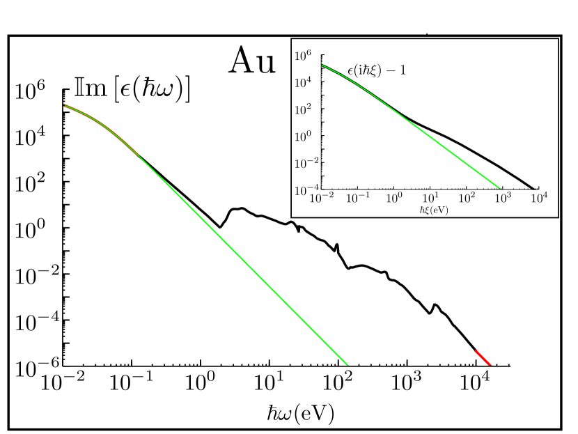
Figure 2: Log-log plot of the imaginary part of the dielectric susceptibility of gold(in black) on real frequencies take from [30]. The extrapolations at low and high frequencies are plotted in red, the Drude model for gold $\epsilon=1-{\omega_{P}^{2}}/{[\omega(\omega+\mathrm{i}\Gamma_{\rm{Au}})]}$ is plotted in green. In the insert, the dielectric susceptibility of gold for imaginary frequencies ($\epsilon(\mathrm{i}\hbar\xi)-1$) obtained from the application of the Kramers-Krönig formula to real data following [31] is plotted in black, while the Drude model of gold is plotted in green.

In the NR model, instead of the microscopic Ohm Law, the direct linear relationship of the electric conductivity with the vector potential is assumed $J_{i}(\omega,\bm{k})=\Pi_{ij}(\omega,\bm{k})A^{j}(\omega,\bm{k})$ [32]. As a consequence, a non-properly regularized conductivity, with the name of ”Non Regularized” conductivity $\sigma_{ij}^{\rm NR}$, is derived as [32][33] (see Eq. (56) in [14])

$$\sigma_{ij}^{{\rm NR}}(\omega,\bm{k}_{\parallel})=\dfrac{\Pi_{ij}(\omega,\bm{k}_{\parallel})}{-\mathrm{i}\omega}.$$ (23)

The explicit analytical form of $\sigma_{ij}^{{\rm NR}}$ can be found in [14], and, in terms of the Polarization Operator, in [20][13] and many others papers. This NR conductivity predicts a dissipation-less current coming from the inter-band contribution of $\sigma_{ij}^{\rm{NR}}(\omega,\bm{k}_{\parallel})$ which has a Plasma behavior (Eq. (A.2) of Appendix A.2) [14].

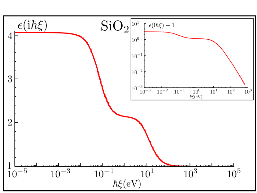
Figure 3: Log-Plot of the dielectric susceptibility of SiO₂ for imaginary frequencies, taken from [30]. In the insert, the dielectric susceptibility of SiO₂ ($\epsilon(\mathrm{i}\hbar\xi)-1$) for imaginary frequencies is represented in a double logarithmic plot.

However, both Kubo and NR conductivities converge to the same local limit. This local limit ($\bm{k}_{\parallel}\to\bm{0}$) of the conductivity for one massive Dirac cone can be analytically written in the $T\to 0$ limit as (see Eq. (93) of [19])

$$\sigma_{xx}^{\rm{L}}(\omega,\Gamma,\mu,T=0) = \mathrm{i}\frac{\sigma_{0}}{\pi}\Bigg{[}\frac{\mu^{2}-\Delta^{2}}{|\mu|}\frac{1}{\Omega}\Theta\left(|\mu|-|\Delta|\right)$$ (24)

$$\!\!\!\!\!\!\!\!\!\!\!\!\!\!\!\!\!\!\!\!\!\!\!\!\!\!\!\!\!+\frac{\Delta^{2}}{M\Omega}-\frac{\Omega^{2}+4\Delta^{2}}{2\mathrm{i}\Omega^{2}}\tan^{-1}\left(\frac{\mathrm{i}\Omega}{2M}\right)\Bigg{]},$$

$$\sigma_{xy}^{\rm{L}}(\omega,\Gamma,\mu,T=0) = \frac{2\sigma_{0}}{\pi}\frac{\eta\Delta}{\mathrm{i}\Omega}\tan^{-1}\left(\frac{\mathrm{i}\Omega}{2M}\right).$$

Note that $\sigma_{0}=\frac{\alpha c}{4}$ is the universal conductivity of graphene ($\alpha=\frac{e^{2}}{\hbar c}$ is the fine structure constant), $\Omega=\hbar\omega+\mathrm{i}\hbar\Gamma$ and $M=\text{Max}\left[|\Delta|,|\mu|\right]$. These results are per Dirac cone and they are consistent with the ones found in [34][35][36][37][38][6][39][40][41]. The first term in $\sigma_{xx}$ corresponds to intra-band transitions, and the last two terms to inter-band transitions. Note that, in the local limit $\bm{k}_{\parallel}=\bm{0}$ one obtains $\sigma_{xx}(\omega,\bm{0})=\sigma_{yy}(\omega,\bm{0})=\sigma_{L}(\omega,\bm{0})=\sigma_{T}(\omega,\bm{0})$, and $\sigma_{xy}(\omega,\bm{0})=-\sigma_{yx}(\omega,\bm{0})=\sigma_{H}(\omega,\bm{0})$. By using the Maldague formula Eq. (22), we can obtain the local conductivity for any temperature using the conductivity given in Eq. (24). From this result, in the $\Delta\to 0$ limit, the Falkovsky model [15] can be derived, as shown in [14].

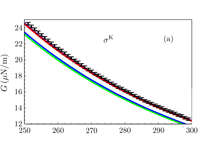
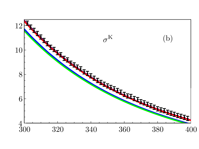
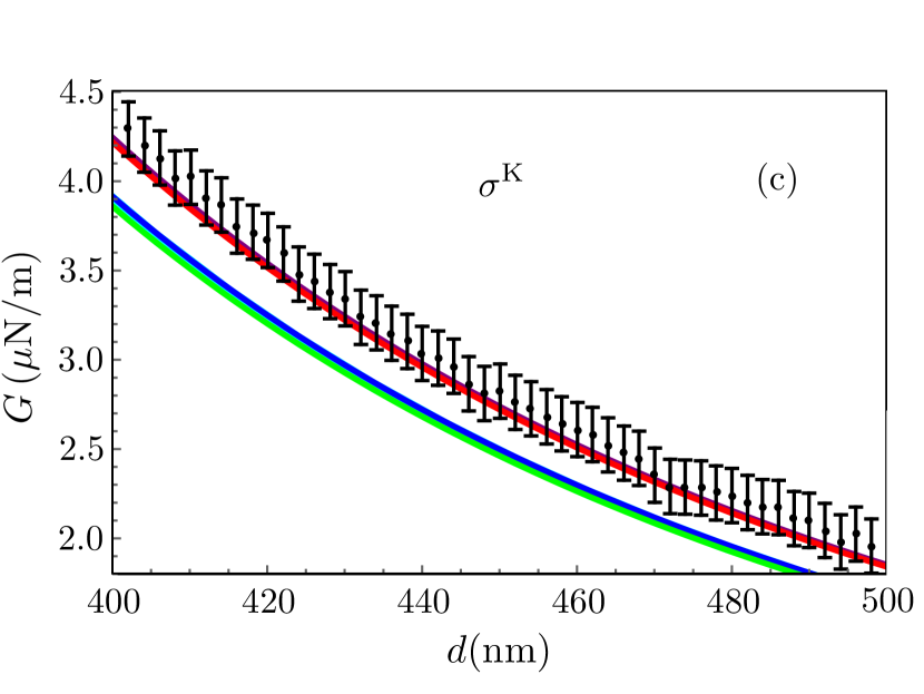
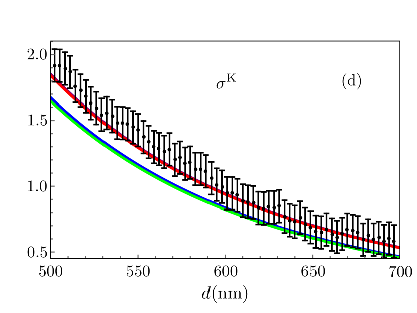
Figure 4: Plots of the CLF gradient $G_{\rm{r}}(d)$ of (25) and as a function of the distance $d$. The experimental data are represented with the black points, the numerical results at $T=294\text{ K}$ are in purple ($\Delta=0\text{ eV}$ and $\mu=0.25\text{ eV}$) and in red ($\Delta=0.1\text{ eV}$ and $\mu=0.23\text{ eV}$), while the results at $T=0\text{ K}$ are in blue ($\Delta=0\text{ eV}$ and $\mu=0.25\text{ eV}$) and green ($\Delta=0.1\text{ eV}$ and $\mu=0.23\text{ eV}$). For the numerical evaluation we used here the general non-local Kubo model $\sigma^{\rm{K}}$ for graphene [19][14] with losses $\hbar\Gamma_{\rm{Gr}}=10^{-3}\text{ eV}$. For the $n=0$ Matasubara term we used the Drude prescription for gold (11), with $\hbar\omega_{P}=9\text{ eV}$ and $\hbar\Gamma_{\rm{Au}}=35\times 10^{-3}\text{ eV}$.

V Numerical calculation of the CLF gradient and comparison with experiments

In this section, we compare the CLF gradient calculated using three different conductivity models (detailed in the previous section) with the experiment [13]. The system consists of an Au-coated microsphere and a graphene sheet deposited on a silica glass (SiO₂) plate, for which we will use exactly the same system parameters used in [13]. As done in [13], we will correct the CLF expressions to take into account the contribution of the roughness of the two surfaces:

$$G_{\rm{r}}(d)=\left[1+10\dfrac{\delta_{s}^{2}+\delta_{g}^{2}}{d^{2}}\right]G(d)$$ (25)

where we will use $\delta_{s}=0.9\text{ nm}$ and $\delta_{g}=1.5\text{nm}$ for the roughness of the metallic sphere and of the graphene, respectively. We note that the roughness correction in this experiment are of $\approx 0.05\%$ at $d=250\text{ nm}$ and of $\approx 0.006\%$ at $d=700\text{ nm}$. The microsphere of diameter $2R=120.7\pm 0.1\mu\text{m}$ is made of hollow glass, and it is coated with a layer of $L=120\pm 3\text{ nm}$ of thickness of Au. The experiment was carried out at $T=294\pm 0.5\text{ K}$, the chemical potential of graphene was measured as $\mu=0.24\pm 0.01\text{eV}$. The SiO₂ substrate induces a non-topological mass gap to the graphene in the interval $m_{G}=(0.01-0.2)\text{ eV}$, corresponding to a Dirac mass $\Delta=m_{G}/2=(0.005-0.1)\text{ eV}$. More experimental details are given in [13].

In our calculations, we use the dielectric permittivity of gold and SiO₂ tabulated in [30], and applied a Kramers-Krönig transformation to obtain the results for imaginary frequencies [31][42], obtaining the results shown in Fig. 2 for gold and in Fig. 3 for SiO₂. For very low frequencies ($n=0$ Matsubara frequency), we have used for gold the Drude model (11) with with $\hbar\omega_{P}=9\text{ eV}$ and $\hbar\Gamma_{\rm{Au}}=35\times 10^{-3}\text{ eV}$.

We compare the experimental results of [13] for the CLF gradient with calculations using three different conductivity models: $\sigma^{\rm{K}}$ [19], $\sigma^{\rm{L}}$ [19][15] and $\sigma^{\rm{NR}}$ [13][20]. See also [14] for a comparison between the 3 different models. Let us start discussing first the results obtained using $\sigma^{\rm{K}}$. In Fig. 4 the experimental results (extracted from the figures in [13]) are plotted together with the theory using the non-local Kubo model $\sigma^{\rm{K}}$ [19]. The experimental data, with its error bars are represented as black points and bars, respectively, and they are compared with the numerical results for four different cases at $T=294\text{ K}$ (purple ($\Delta=0\text{ eV}$ and $\mu=0.25\text{ eV}$) and red ($\Delta=0.1\text{ eV}$ and $\mu=0.23\text{ eV}$)) and at $T=0\text{ K}$ (blue ($\Delta=0\text{ eV}$ and $\mu=0.25\text{ eV}$) and green ($\Delta=0.1\text{ eV}$ and $\mu=0.23\text{ eV}$)).

We can see that the theory predictions at $T=294\text{ K}$ are qualitatively in good agreement with the experimental results. To be more quantitative we represent in Fig. 5 the relative difference

$$\mathcal{D}(Exp,Theo)=\left|\dfrac{Exp-Theo}{Exp}\right|$$ (26)

between the experimental result and each one of the four theory curves showed in Fig. 4, using the same color code. The black curve is the relative difference between the lower experimental error bar and the experimental result in Fig. 4.

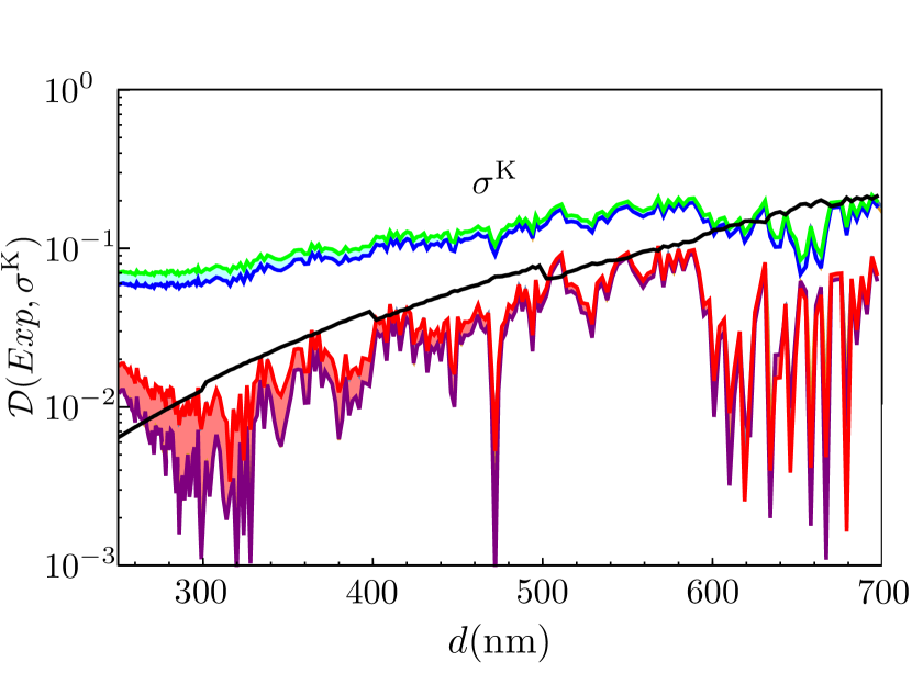
Figure 5: Logarithmic Plot of the relative difference $\mathcal{D}(Exp,\sigma^{\rm{K}})$ (Eq. (26)) of the theoretical predictions using the non-local Kubo model $\sigma^{\rm{K}}$ with the experimental result of [13]. The numerical results at $T=294\text{ K}$ are in purple ($\Delta=0\text{ eV}$) and in red ($\Delta=0.1\text{ eV}$), while the results at $T=0\text{ K}$ are in blue ($\Delta=0\text{ eV}$) and green ($\Delta=0.1\text{ eV}$), the same as in Fig. 4. The black curve is the error bar compared with the experimental value of each experimental point $\mathcal{D}(Exp,Exp\text{ lower bar})$. Theoretical values below this black curve show cases when the theoretical results are inside the experimental error-bars. We can observe a small discrepancy at short distances.

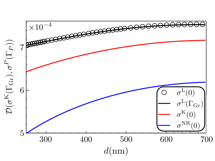
Figure 6: Relative difference $\mathcal{D}(\sigma^{\rm{K}}(\Gamma_{\rm{Gr}}),\sigma^{X}(\Gamma_{X}))$ Eq. (26) with $X=\{\rm{L,K,NR}\}$ of the CLF gradient $G(d)$ using: $\sigma^{\rm{L}}$ (with losses $\Gamma_{\rm{L}}=\Gamma_{\rm{Gr}}$, black full line, and without losses $\Gamma_{\rm{L}}=0$, black circles), $\sigma^{\rm{K}}$ without losses $\Gamma_{\rm{K}}=0$ (red line) and $\sigma^{\rm{NR}}$ (blue line) with $\Gamma_{\rm{NR}}=0$, all compared with the CLF gradient using the non-local Kubo model $\sigma^{\rm{K}}$ with losses $\Gamma_{\rm{K}}=\Gamma_{\rm{Gr}}$. Here $T=294\text{ K}$, $\Delta=0\text{ eV}$ and $\mu=0.25\text{ eV}$.

All points below the black curve are consistent numerical predictions for the experimentally measured derivative of the Force experienced between the gold sphere and the graphene-covered SiO₂ plate. We can observe that the effect of temperature is distinguished by the experiment, the blue and green curves (predictions performed in the $T\to 0$ limit, with Eq. (2)) do not fit the experimental results for distances $d<600\text{ nm}$, while the predictions performed taking into account the temperature of the experiment at $T=294\text{ K}$ (red and purple curves, with Eq. (1)) fit the experimental results.

Let us now analyze and compare, in Fig. 6, the CLF gradient theory prediction using the other conductivity models. We keep the same experimental conditions for the three cases ($T=294\text{ K}$, and graphene with $\Delta=0\text{ eV}$ and $\mu=0.25\text{ eV}$). For gold, we use the Drude prescription here, the losses of gold are set to $\hbar\Gamma_{\rm{Au}}=35\times 10^{-3}\text{ eV}$, and the losses of graphene are set to $\hbar\Gamma=10^{-3}\text{ eV}$. The results obtained with the Non-Local Kubo $\sigma^{\rm{K}}$ without losses, Local $\sigma^{\rm{L}}$ (with and without losses) and NR $\sigma^{\rm{NR}}$ conductivity models are practically identical, having a relative difference smaller than $10^{-3}$ with respect to predictions using $\sigma^{\rm{K}}$ with losses $\hbar\Gamma=10^{-3}\text{ eV}$. We can conclude that the experiment is performed in a region of parameters where the local model $\sigma^{\rm{L}}$ gives results very close to the one obtained with the non-local Kubo $\sigma^{\rm{K}}$, hence the experiment only test the graphene conductivity in the local regime. As reported in [14], the $\sigma^{\rm{NR}}$ is correct (only) in the local limit when the effect of losses is negligible, and this is confirmed in Fig. 6 where we see that $\sigma^{\rm{NR}}$ gives results practically identical to the ones of $\sigma^{\rm{K}}$ and $\sigma^{\rm{L}}$.

Due to the equivalence of the three conductivity models in this given (local) experimental regime, the corresponding figures on the theory-experiment comparison obtained using the $\sigma^{\rm{L}}$ and $\sigma^{\rm{NR}}$ models will be strictly indistinguishable from Fig. 4 and Fig. 5, as it is explicitly shown in the Appendices B.1 and B.2.

It is worth noticing that, in the theory-experiment comparison of Fig. 4, the theory curves are slightly lower than the theory curves published in [13], essentially at short distances ($d<280\text{ nm}$). Since we just shown that, for this experimental parameters, the graphene model $\sigma^{\rm{NR}}$ used [13] provides a CLF gradient prediction practically identical to the one obtained with $\sigma^{\rm{K}}$ (and $\sigma^{\rm{L}}$), this discrepancy cannot originate from to the model used for the graphene conductivity. It can only be due to possible differences in the numerical evaluation of the CLF gradient expression (different numerical accuracy in the wavevector integration and Matsubara sum Eq. (1), and/or differences in the numerical handling of the gold/SiO₂ dielectric functions).

V.1 Effect of the chemical potential

In figure Fig. 4 we see that the theory predictions are compatible with the experimental result almost everywhere. Nonetheless, in particular at short distances, the experimental results are systematically higher than the theory predictions. This systematic difference may be due to several experimental reasons which are beyond our control and that we cannot investigate systematically. We consider in this section just one of the possible origin for that difference, just to have an idea of the sensibility of the theory to different values used for the chemical potential. In Fig. 7, we study the CLF gradient as a function of the chemical potential $\mu$, for a fixed separation distance $d=251.1\text{ nm}$, and for two different values of the Dirac mass $\Delta$ used in [13] (green line for $\Delta=0\text{ eV}$ and the red line for $\Delta=0.1\text{ eV}$). The chemical potential used in [13] was $\mu=0.25\text{ eV}$ when $\Delta=0\text{ eV}$ and $\mu=0.23\text{ eV}$ when $\Delta=0.1\text{ eV}$. Fig. 7 shows that for values of the chemical potential around $\mu=0.395\text{ eV}$ the theory-experiment agreement largely improves.

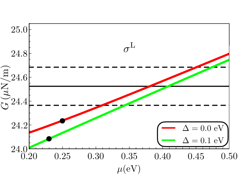
Figure 7: Linear plot of the CLF derivative $G$ as a function of the chemical potential $\mu$ for a fixed distance of $d=251.1\text{ nm}$ at $T=294\text{ K}$. The red curve is the case with $\Delta=0\text{ eV}$, while the green curve is the case with $\Delta=0.1\text{ eV}$. The black line is the experimental results of [13] at $d=(251.1\pm 0.6)\text{ nm}$, and the black dotted lines are the lower and upper limits of the error bars of this experimental value. We have indicated with black dots the numerical values obtained for $\mu=0.25\text{ eV}$ when $\Delta=0$ and for $\mu=0.23\text{ eV}$ when $\Delta=0.1\text{ eV}$ as the ones used in [13] and in the rest of the text.

V.2 Effect of losses

In this subsection we discuss the effect that losses in graphene [14] have in the experiment [13] keeping the losses of gold as $\hbar\Gamma_{\rm{Au}}=35\times 10^{-3}\text{ eV}$. Losses in graphene are a small non-zero quantity, and we assume that their effect on the electric conductivity can be well approached with the finite lifetime approximation by a constant imaginary dissipation rate $\Gamma=\tau^{-1}$ [26][43][44][45][46], where $\tau\backsim 6\times 10^{-13}\text{ s}$ is estimated in [26][27]. The model we have that can handle losses is the Kubo model [19], either in the local limit given in Eq. (24) or the general non-local case given in Eq. (A.1). Then we compare the experimental results with a dissipation time of $\tau\backsim 6\times 10^{-13}\text{ s}$ with the zero-dissipation result $\tau\to\infty$. The results are shown in Fig. 8, where we observe that, for the conditions of the experiment and considered distances, the relative error is lower than $10^{-3}$, and therefore, the effects of losses of graphene cannot be observed in the experiment.

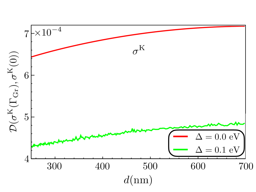
Figure 8: Relative difference $\mathcal{D}(\sigma^{\rm{K}}(\Gamma_{\rm{Gr}}),\sigma^{\rm{K}}(0))$ Eq. (26) of $\sigma^{\rm{K}}$ without losses ($\Gamma=0$ for graphene) compared with the case with losses ($\Gamma=\Gamma_{\rm{Gr}}$ for graphene). The red curve is the case with $T=294\text{ K}$, $\Delta=0\text{ eV}$ and $\mu=0.25\text{ eV}$, while the green curve is the case with $T=294\text{ K}$, $\Delta=0.1\text{ eV}$ and $\mu=0.23\text{ eV}$. For the $n=0$ Matsubara term we have used the Drude prescription for gold, with $\hbar\Gamma_{\rm{Au}}=35\times 10^{-3}\text{ eV}$.

VI Drude vs. Plasma

In this section we compare the results by using the Drude and Plasma prescriptions to calculate the Casimir effect. In experiments on the CLF, it has been shown that the use of a Plasma prescription in the Casimir-Lifshitz theory (use of the zero losses limit of the metallic objects of the systems in the zero frequency term) provides a better theory experimental agreement than with a Drude model (i.e. use of non-zero losses for metals in the zero frequency term) [47][48][49]. This contrasts with the natural choice of the Drude model for normal metals, where in the limit of zero frequency, losses are present if a DC electric field is applied, and some experiments fit better with this prescription [50].

As the use of a Plasma or Drude model could in principle modify the theoretical prediction of the results of the experiment, we apply a detailed study here of the classical limit ($n=0$ Matsubara term) of the CLF gradient $G_{\rm{cl}}$ Eq. (3), which is the term affected by the choice between the two prescriptions.

In the following we will need to calculate the $\xi\rightarrow 0$ of graphene conductivity, and we can have typically three behaviors:

$$\bar{\sigma}_{P}(\xi,\bm{k}_{\parallel}) \underset{\xi\to 0}{\approx} \dfrac{\bar{\sigma}_{P,-1}(\bm{k}_{\parallel})}{\xi}+\mathcal{O}\left[\xi^{0}\right]$$ (27)

$$\bar{\sigma}_{P}(\xi,\bm{k}_{\parallel}) \underset{\xi\to 0}{\approx} \bar{\sigma}_{P,0}(\bm{k}_{\parallel})+\mathcal{O}\left[\xi^{1}\right]$$ (28)

$$\bar{\sigma}_{P}(\xi,\bm{k}_{\parallel}) \underset{\xi\to 0}{\approx} \bar{\sigma}_{P,1}(\bm{k}_{\parallel})\xi+\mathcal{O}\left[\xi^{2}\right]$$ (29)

defining the constant $\bar{\sigma}_{P,0}$, $\bar{\sigma}_{P,-1}$ and $\bar{\sigma}_{P,1}$, where $P=\{\rm{L,T}\}$ are the two polarizations.

VI.1 Local model

VI.1.1 Drude metal model

When losses are considered in the local model for the conductivity of graphene (Eq. (24)), one can show that the $\xi\to 0$ behavior of $\sigma_{P}(\xi)$ is given by Eq. (28) as

$$\bar{\sigma}_{P,0}^{\rm{L}} = \frac{\alpha}{2}\Bigg{[}\frac{\mu^{2}-\Delta^{2}}{|\mu|}\frac{1}{\hbar\Gamma}\Theta\left(|\mu|-|\Delta|\right)$$ (30)

$$+\frac{\Delta^{2}}{M\hbar\Gamma}+\frac{4\Delta^{2}-\hbar^{2}\Gamma^{2}}{2\hbar^{2}\Gamma^{2}}\tan^{-1}\left(\frac{\hbar\Gamma}{2M}\right)\Bigg{]}.$$

for any polarization $P=\{\rm{L,T}\}$ at $T=0$. To obtain the result for any finite temperature we should use the Maldague formula Eq. (22). Therefore, the Fresnel reflection matrix for SiO₂ covered by graphene $\mathbb{R}^{\rm{Gr}}$ and for gold $\mathbb{R}^{\rm{Au}}$ with losses are equal to

$$\displaystyle\lim_{\xi\to 0}\mathbb{R}^{\rm{Gr}}=\displaystyle\lim_{\xi\to 0}\mathbb{R}^{\rm{Au}}=\left(\begin{array}[]{cc}0&0\\ 0&1\end{array}\right).$$ (33)

In this case, the $n=0$ Matsubara CLF gradient is exactly

$$G_{\rm{cl}}(d)=G_{\rm{cl},\rm{pp}} = k_{B}TR\displaystyle\int_{0}^{\infty}\mathrm{d}k_{\parallel}k_{\parallel}^{2}\dfrac{e^{-2dk_{\parallel}}}{1-e^{-2dk_{\parallel}}}$$ (34)

$$= -\frac{k_{B}TR\zeta(3)}{4d^{3}},$$

which is the Drude result for the thermal CLF gradient.

VI.1.2 Plasma model

If we artificially neglect losses in the local model for the conductivity of graphene Eq. (24), we obtain a Plasma model

$$\bar{\sigma}_{P}^{\rm{L}}(\xi)\underset{\xi\to 0}{\approx}\dfrac{\bar{\sigma}_{P,-1}^{\rm{L}}}{\xi}$$ (35)

with

$$\bar{\sigma}_{P,-1}^{\rm{L}}=\dfrac{\alpha c}{4\pi\hbar}\dfrac{\mu^{2}-\Delta^{2}}{|\mu|}\Theta\left(|\mu|-|\Delta|\right)$$ (36)

for any polarization $P=\{\rm{L,T}\}$ at $T=0$. To obtain the result for any finite temperature we should use the Maldague formula Eq. (22). Therefore, the Fresnel reflection matrix tends to

$$\displaystyle\lim_{\xi\to 0}\mathbb{R}^{\rm{Gr}}=\left(\begin{array}[]{cc}\dfrac{-\bar{\sigma}_{T,-1}}{ck_{\parallel}+\bar{\sigma}_{T,-1}}&0\\ 0&1\end{array}\right)$$ (39)

In the Plasma prescription, the zero frequency limit of the Fresnel matrix for gold $\mathbb{R}^{\rm{Au}}$ is given by Eq. (18). In this case, the CLF derivative is the sum of the contribution of the 2 unmixed polarizations

$$\!\!\!\!\!\!\!\!\!\!\!\!\!\!\!\!\!\!\!\!G_{\rm{cl}}(d) = G_{\rm{cl},\rm{ss}}+G_{\rm{cl},\rm{pp}}$$ (40)

$$\!\!\!\!\!\!\!\!\!\!\!\!\!\!\!=k_{B}TR\displaystyle\int_{0}^{\infty}\mathrm{d}k_{\parallel}k_{\parallel}^{2}\text{Tr}\left(\dfrac{\mathbb{R}^{\rm{Au}}\mathbb{R}^{\rm{Gr}}e^{-2dk_{\parallel}}}{\mathbbm{1}-\mathbb{R}^{\rm{Au}}\mathbb{R}^{\rm{Gr}}e^{-2dk_{\parallel}}}\right),$$

where the $\rm{pp}$ contribution equals to the Drude result given in Eq. (34)

$$G_{\rm{cl},\rm{pp}}(d)=-\frac{k_{B}TR\zeta(3)}{4d^{3}}.$$ (41)

For the $\rm{ss}$ polarization, we have

$$\!\!\!G_{\rm{cl},\rm{ss}}(d)=k_{B}TR\!\!\displaystyle\int_{0}^{\infty}\mathrm{d}k_{\parallel}k_{\parallel}^{2}\text{Tr}\left(\dfrac{R_{\rm{ss}}^{\rm{Au}}R_{\rm{ss}}^{\rm{Gr}}e^{-2dk_{\parallel}}}{1-R_{\rm{ss}}^{\rm{Au}}R_{\rm{ss}}^{\rm{Gr}}e^{-2dk_{\parallel}}}\right)\!\!,$$ (42)

for which one we can distinguishes three regions:

$$G_{\rm{cl},\rm{ss}}(d) \underset{d>d_{0}}{\approx} -\frac{k_{B}TR\zeta(3)}{4d^{3}},$$ (43)

$$G_{\rm{cl},\rm{ss}}(d) \underset{d\ll\frac{c}{\omega_{P}}}{\approx} -\frac{k_{B}TR\omega_{P}^{2}}{2c^{2}d_{0}}\log\left(\frac{\sqrt{2}e^{\gamma}\omega_{P}d}{c}\right)\!\!,$$ (44)

$$G_{\rm{cl},\rm{ss}}(d) \underset{\frac{c}{\omega_{P}}<d<d_{0}}{\approx} -\frac{k_{B}TRc^{2}}{8\pi d_{0}d^{2}}\left(1-\dfrac{2c}{d\omega_{P}}\right),$$ (45)

where

$$d_{0}=\dfrac{2\hbar c}{\alpha}\dfrac{|\mu|}{\mu^{2}-\Delta^{2}}=2.57\times 10^{-4}\text{ m}.$$ (46)

For gold, we have $c/\omega_{P}\approx 22\text{ nm}$, therefore, for the considered experiment, the $c/\omega_{P}<d<d_{0}$ is the relevant limit and the $\rm{ss}$ polarization has a negligible contribution that, in principle, will be very difficult to be measured, as can be observed in Fig. 9. We conclude that, for the considered distances, Drude and Plasma prescriptions practically coincide when the Local model $\sigma^{\rm{L}}$ is used.

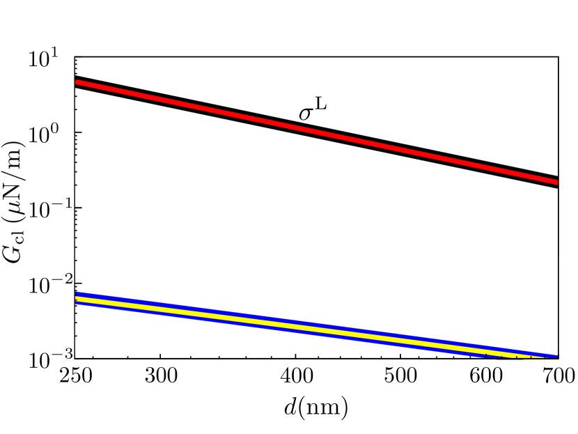
Figure 9: Double logarithmic plot of the $n=0$ Matsubara contribution of the CLF gradient $G_{\rm{cl}}$ calculated with the local model $\sigma^{\rm{L}}$ as a function of the distance $d$. The Black thick curve and the red curve are the results of the Plasma (Eq. (40), using Eqs. (41) and (42)) and Drude (Eq. (34)) prescriptions, respectively. The blue curve is the exact result for the $\rm{ss}$ component of the Plasma prescription defined in Eq. (42), and the yellow curve is the approximation of Eq. (42) for intermediate distances, when $c/\omega_{P}<d<d_{0}$.

VI.2 Non-Local Kubo model

VI.2.1 Drude metal model

When losses $\hbar\Gamma>0$ are considered in the non-local Kubo model, one can find that the $\xi\to 0$ limit of $\bar{\sigma}_{P}(\xi)$ tends to $\bar{\sigma}_{P,0}$ of Eq. (28) given by Eq. (A.1). It is easy to check that $0<\bar{\sigma}_{P,0}<\infty$ for any polarization $P=\{\rm{L,T}\}$ and temperature $T$. Therefore, the Fresnel reflection matrix for SiO₂ covered by graphene and for gold are given by Eq. (33). As a result, the zero Matsubara CLF gradient is the usual Drude result given in Eq. (34).

VI.2.2 Plasma model

If we artificially neglect the effect of losses in the non-local Kubo model for the conductivity of graphene making $\hbar\Gamma=0$, we obtain Eq. (A.1) in the $T=0$ limit, and we have to apply the Maldague formula (Eq. (22)) to those conductivities to obtain the corresponding finite $T$ result.

In this case, the longitudinal conductivity behaves like Eq. (29), while the transversal conductivity behaves like Eq. (28), as a consequence, the zero frequency limit of the Fresnel reflection matrix is

$$\displaystyle\lim_{\xi\to 0}\mathbb{R}^{\rm{Gr}}=\left(\begin{array}[]{cc}0&0\\ 0&\dfrac{\epsilon_{1}-1+2ck_{\parallel}\bar{\sigma}_{L,1}}{\epsilon_{1}+1+2ck_{\parallel}\bar{\sigma}_{L,1}}\end{array}\right)$$ (49)

where $\displaystyle\lim_{\xi\to 0}\epsilon_{SiO_{2}}(\xi)=\epsilon_{1}$, and we have used that $\bar{\sigma}_{L,1}>0$ and $0\leq\bar{\sigma}_{T,0}<\infty$ for all $k_{\parallel}>0$. It is worth noting that for $k_{\parallel}=0$, one has $\mathbb{R}_{ss}^{\rm{Gr}}(\xi\to 0,k_{\parallel}\to 0)\neq 0$ (given by Eq. (39)), but this anomalous term is irrelevant for the computation of the CLF, because: i) this result does not generate a pole in the integrand, and ii) it is only obtained in a set of zero measure, therefore, it cannot contribute to the calculation of the CLF gradient and we must use Eq. (49) in the Lifshitz formula. By considering the lowest order expansion in $k_{\parallel}\to 0$, we have

$$\bar{\sigma}_{L,1}(k_{\parallel}) \underset{k_{\parallel}\to 0}{\approx} \alpha\dfrac{4|\mu|-|\Delta|}{\hbar v_{F}^{2}k_{\parallel}^{2}}+\mathcal{O}\left[\dfrac{1}{k_{\parallel}}\right],$$ (50)

where we have assumed that $|\mu|>|\Delta|$. As a consequence, the classical limit of the CLF gradient with the plasma prescription is approached by

$$\!\!\!\!\!\!\!\!\!\!\!\!\!\!G_{\rm{cl}}(d)\approx$$ (51)

$$\!\!\!\!\!\!\!\!\!\!\!\!\!\!\!\!\!\!\!\!\!\!\!\!-\frac{k_{B}TR\zeta(3)}{4d^{3}}\left(1-\dfrac{6\hbar v_{F}^{2}}{\alpha c(4|\mu|-|\Delta|)d}+\mathcal{O}\left[\dfrac{1}{d^{2}}\right]\right).$$

This result is always strictly smaller, but very close to the one obtained with the non-local Drude model Eq. (34). So we conclude that also when we use the non-local Kubo model, the effect of Plasma prescription is irrelevant in this experiment, as can be observed in Fig. 10.

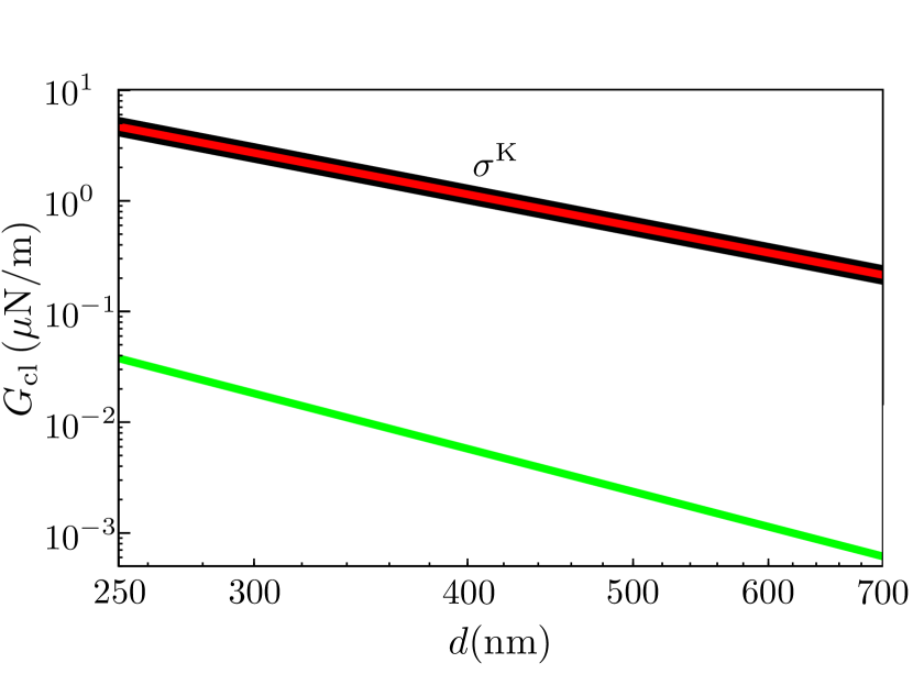
Figure 10: Double logarithmic plot of the $n=0$ Matsubara term of the CLF gradient $G_{\rm{cl}}$ calculated with the Kubo model $\sigma^{\rm{K}}$ as a function of the distance $d$. The Black thick curve is the numerical results using the Plasma prescription (Eq. (40) using Eq. (18) for $\mathbb{R}^{\rm{Au}}$ and Eq. (49) for $\mathbb{R}^{\rm{Gr}}$). The red curve is the numerical results using the Drude prescription, given by Eq. (34). The green curve is the difference between the Plasma (black) and Drude (red) results.

VI.3 Non-Regularized model

In the case of the NR model, one can find that the $\xi\to 0$ limit of the Longitudinal conductivity can be approached using Eq. (65), from where we obtain that

$$\bar{\sigma}_{L}^{\rm{NR}}(\xi)\underset{\xi\to 0}{\approx}\bar{\sigma}_{L,1}\xi,$$ (52)

with $\bar{\sigma}_{L}^{(1)}$ given in Eq. (66), and the Transversal conductivity, using Eq. (A.2) can be approached in the $\xi\to 0$ limit as

$$\bar{\sigma}_{T}^{\rm{NR}}(\xi)\underset{\xi\to 0}{\approx}\frac{\bar{\sigma}_{T,-1}}{\xi},$$ (53)

with $\sigma_{T,-1}$ given in Eq. (74). When $|\mu|>|\Delta|$, at room temperature, one can show that those results can be safely approximated by

$$\bar{\sigma}_{T,-1} \approx \alpha v_{F}k_{\parallel}\frac{\pi}{2}\Theta\left(k_{\parallel}-K\right),$$ (54)

$$\bar{\sigma}_{L,1} \underset{k_{\parallel}\to 0}{\approx} \alpha\dfrac{4|\mu|-|\Delta|}{\hbar v_{F}^{2}k_{\parallel}^{2}},$$ (55)

with $K=2\sqrt{\mu^{2}-\Delta^{2}}/(\hbar v_{F})$. Therefore, for SiO₂ covered by graphene, the zero frequency Fresnel coefficients are

$$\lim_{\xi\to 0}R_{\rm{ss}}^{\rm{Gr}} = \dfrac{-\bar{\sigma}_{T,-1}}{ck_{\parallel}+\bar{\sigma}_{T,-1}}\approx\dfrac{-\frac{\pi\alpha v_{F}}{2c}}{1+\frac{\pi\alpha v_{F}}{2c}}\Theta\left(k_{\parallel}-K\right)$$ (56)

$$\lim_{\xi\to 0}R_{\rm{pp}}^{\rm{Gr}} = \dfrac{\epsilon_{1}-1+2ck_{\parallel}\bar{\sigma}_{L,1}}{\epsilon_{1}+1+2ck_{\parallel}\bar{\sigma}_{L,1}}$$ (57)

where we have used that, in this model $\sigma_{T,-1}\neq 0$ only for $k_{\parallel}>K=2\sqrt{\mu^{2}-\Delta^{2}}/(\hbar v_{F})$. As a result, the integral contained in the $n=0$ Matsubara term of the CLF gradient only has contributions of those large wavevectors. For those cases, the Fresnel coefficients of gold can be approximated as

$$\lim_{\xi\to 0}R_{\rm{ss}}^{\rm{Au}} \underset{k_{\parallel}>K}{\approx} -\left(\frac{\omega_{P}}{2ck_{\parallel}}\right)^{2}$$ (58)

$$\lim_{\xi\to 0}R_{\rm{pp}}^{\rm{Au}} = 1$$ (59)

and the $n=0$ Matsubara term of the CLF gradient due to the $\rm{ss}$ Fresnel coefficients can be approximated by

$$G_{\rm{cl},\rm{ss}} \approx k_{B}TR\frac{\omega_{P}^{2}\pi\alpha v_{F}}{16c^{3}}\dfrac{e^{-2dK}}{d}.$$ (60)

In the experiment [13], $\Delta=0.1\text{ eV}$ and $\mu=0.23\text{ eV}$, therefore we have $K^{-1}=d_{0}=\dfrac{\hbar v_{F}}{2\sqrt{\mu^{2}-\Delta^{2}}}\approx 1.6\text{ nm}$ (and $K^{-1}\approx 1.3\text{ nm}$ for $\Delta=0$ and $\mu=0.25\text{ eV}$). In Fig. 11, the contribution of $G_{\rm{cl},\rm{ss}}$ to the experimental result for the conditions and distances of the experiment [13] can be observed. This $n=0$ Matsubara term is exponentially neglected for the experimentally relevant distances, therefore, even when there is a Plasma contribution to the $n=0$ Matsubara term, in practice it cannot contribute to the final result.

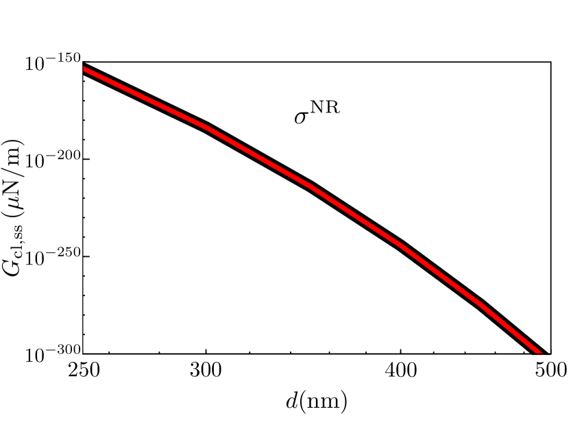
Figure 11: Double logarithmic plot of the $n=0$ Matsubara term of the CLF gradient $G_{\rm{cl},\rm{ss}}$ calculated with the NR model $\sigma^{\rm{NR}}$ as a function of the distance $d$. The black thick curve is the numerical result obtained using Eq. (40) with Eq. (18) for $\mathbb{R}^{\rm{Au}}$ and Eq. (56) and Eq. (57) for $\mathbb{R}^{\rm{Gr}}$, and the red curve is the approximation given in Eq. (60).

The $\rm{pp}$ term of the Fresnel reflection matrix is modified into

$$\displaystyle\lim_{\xi\to 0}\mathbb{R}_{\rm{pp}}^{\rm{Gr}}=\dfrac{\epsilon_{1}-1+2ck_{\parallel}\bar{\sigma}_{L,1}}{\epsilon_{1}+1+2ck_{\parallel}\bar{\sigma}_{L,1}}$$ (61)

We remark that this reflection coefficient is the same as the one obtained with the non-local Kubo model $\sigma^{\rm{K}}$ when the Plasma prescription is used and also the expression for $\bar{\sigma}_{L,1}$ is the same (compare Eq. (55) with Eq. (50)), then we obtain that $G_{\rm{cl},\rm{pp}}(d)$ is equal to Eq. (51).

This result cannot be distinguished in the experiment from the usual Drude $n=0$ Matsubara term of the CLF gradient, as shown in Fig. 10 when losses are considered. We conclude that, with the NR model, the Plasma and Drude prescriptions provides the same numerical result, to all practical extents.

In conclusion, for any of the three models used for the graphene conductivity, and for both Drude or Plasma prescriptions, the $n=0$ Matsubara term always provides a numerical result indistinguishable from the theoretical Drude result given in (34), i.e. the usual Drude result for the thermal CLF. Hence it is not possible, in this experiment, to distinguish the Drude from the Plasma prescription.

VII Conclusion

We have compared the CLF gradient experimental results [13] between a gold sphere and a graphene-coated plate with the Lifshitz theory using three different models for the electric conductivity of graphene. In particular, we have considered the general non-local Kubo model, the local limit of the Kubo model, and the non-regularized and lossless model used in [13], recently shown to be not correct [14] apart from the local limiting case, where it has been shown to exactly provide the local Kubo expression (once also losses are included). We show that the non-local Kubo and the local Kubo models provide practically identical predictions for the CLF gradient when calculated using the parameters of the experiment [13]. Hence that experiment is sensible only to local effects of graphene. The non-regularized model also produces results practically identical to the two other cases, and this is since it is applied in the only region where it is correct, i.e. the local regime. There, the three models provide results for the CLF gradient with a relative difference smaller than $10^{-3}$. Thanks to the natural presence of losses in the Kubo model, we have also tested the effect of losses in graphene conductivity, and we have shown that the CLF gradient is practically insensitive to graphene losses for the parameters used in experiment [13]. This also explains why, again, the non-regularized lossless model still provides results very similar to that of the Kubo model for the given experimental parameters. Finally, we have investigated the effect of using a Plasma model for both gold and graphene, in comparison with the correct Drude/Kubo models including losses at zero frequency. We find that, for the experimental parameters [13], the Plasma models provide results practically identical to the Drude ones.

In conclusion, we show that the extremely simple local Kubo model given by $\sigma_{L}(\omega,\bm{0})=\sigma_{T}(\omega,\bm{0})=\sigma_{xx}(\omega,\bm{0})$ of Eq. (24) together with Eq. (22), explicitly depending on Dirac mass, chemical potential, losses and temperature, is largely enough to fully describe the experimental results in [13], and can be safely and effectively used for future comparisons with all classical experimental configurations.

For the future, it would be interesting to compare the Kubo model with ab-initio ones [51], and to study the effects of graphene in NEMS/MEMS based experimental structures [52] where non-locality might possibly play some role in really extreme conditions.

Appendix A Low frequency limit of the Kubo and of the non-regularized graphene conductivity models.

In section VI we analyzed the difference between the Drude and Plasma prescription on the calculation of the CLF gradient. To this extent we need to apply such prescriptions to the $n=0$ Matsubara term, and hence we need to calculate the low frequency limit of the graphene non-local Kubo conductivity and of the NR conductivity. In this appendix we derive such limits.

A.1 Low frequency limit of non-local Kubo conductivity

Here we derive the low frequency limit of the graphene non-local Kubo conductivity [19][14]. For the Plasma prescription, we will also need to discard losses, hence we set $\xi\to 0$ with $\Gamma\to 0$ while for the Drude prescription we set $\xi\to 0$ with $\Gamma\neq 0$. In the $T=0$ limit we have:

$$\lim_{\Omega\to 0}\sigma_{T}^{\rm{K}}(\Omega,k_{\parallel}) = \frac{\alpha c}{\pi}\frac{\tilde{K}^{2}}{\tilde{k}_{\parallel}\sqrt{\tilde{K}^{2}-\tilde{k}_{\parallel}^{2}}}\Theta\left(\tilde{K}-\tilde{k}_{\parallel}\right)\Theta(|\mu|-|\Delta|)$$

$$\sigma_{L}^{\rm{K}}(\Omega,k_{\parallel}) \underset{\Omega\to 0}{\approx} 0+\Omega\sigma_{L,1}(k_{\parallel})$$

$$\lim_{\Omega\to 0}\sigma_{H}^{\rm{K}}(\Omega,k_{\parallel}) = -\frac{\alpha c}{2\pi}\frac{\eta\Delta}{\tilde{k}_{\parallel}}\left[\Theta(|\Delta|-|\mu|)\tan^{-1}\left(\frac{\tilde{k}_{\parallel}}{2|\Delta|}\right)+\Theta(|\mu|-|\Delta|)\cos^{-1}\left(\frac{2|\mu|}{\sqrt{\tilde{k}_{\parallel}^{2}+4\Delta^{2}}}\right)\right]$$

$$\sigma_{L,1}(k_{\parallel}) = \frac{\alpha c}{2\pi}\frac{\hbar}{2\tilde{k}_{\parallel}}\left[\frac{|\Delta|}{\tilde{k}_{\parallel}}+\frac{\tilde{k}_{\parallel}^{2}-4\Delta^{2}}{2\tilde{k}_{\parallel}^{2}}\tan^{-1}\left(\frac{\tilde{k}_{\parallel}}{2|\Delta|}\right)+\Theta(|\mu|-|\Delta|)\left(2\frac{|\mu|-|\Delta|}{\tilde{k}_{\parallel}}+\frac{4\Delta^{2}-\tilde{k}_{\parallel}^{2}}{4\tilde{k}_{\parallel}^{2}}X\right)\right]$$

$$X = \Theta\left(\tilde{k}_{\parallel}^{2}-\tilde{K}^{2}\right)\tan^{-1}\left(2\frac{|\mu|\tilde{k}_{\parallel}-|\Delta|\sqrt{\tilde{k}_{\parallel}^{2}-\tilde{K}^{2}}}{4|\Delta||\mu|+\tilde{k}_{\parallel}\sqrt{\tilde{k}_{\parallel}^{2}-\tilde{K}^{2}}}\right)+\Theta\left(\tilde{K}^{2}-\tilde{k}_{\parallel}^{2}\right)\tan^{-1}\left(\frac{\tilde{k}_{\parallel}}{2|\Delta|}\right)$$ (62)

where $\Omega=\omega+\mathrm{i}\Gamma$, $\tilde{k}_{\parallel}=\hbar v_{F}k_{\parallel}$ and $\tilde{K}=\hbar v_{F}K=2\sqrt{\mu^{2}-\Delta^{2}}$. We have to apply the Maldague formula, given in Eq. (22) to obtain the corresponding finite $T$ results.

A.2 Low frequency limit of non-regularized conductivity

Here we are derive the low frequency limit of the graphene conductivitites for the NR model [20]. We start with the definition of the auxiliary functions

$$\Psi(x,y)=2\left[y\sqrt{1+x^{2}-y^{2}}+\left(1-x^{2}\right)\tan^{-1}\left(\tfrac{\sqrt{1+x^{2}-y^{2}}}{y}\right)\right],$$ (63)

$$\Psi(x)=\displaystyle\lim_{y\to x}\Psi(x,y)=2\left[x+(1-x^{2})\tan^{-1}\left(\frac{1}{x}\right)\right],$$ (64)

From [14], the longitudinal conductivity is

$$\sigma_{L}^{\rm{NR}} = \frac{\alpha c\lambda\Psi\left(\delta\right)}{4\pi}+\frac{\alpha c\Xi\tilde{\theta}_{z}}{\pi\tilde{k}_{\parallel}^{2}}\int_{\delta}^{\infty}\mathrm{d}uN_{\mu}\left(\tfrac{\tilde{\theta}_{z}}{2}u\right)\left(1-\mathbb{R}\text{e}\left[\frac{1-u^{2}+2\mathrm{i}\lambda u}{\sqrt{1-u^{2}+2\mathrm{i}\lambda u+\left(1-\lambda^{2}\right)\delta^{2}}}\right]\right),$$ (65)

$$\sigma_{L}^{\rm{NR}} \underset{\xi\to 0}{\approx} \frac{\alpha c}{4\pi}\frac{\Xi}{\tilde{k}_{\parallel}}\left[\Psi(x)+4\int_{x}^{\infty}\mathrm{d}uN_{\mu}\left(\tfrac{\tilde{k}_{\parallel}}{2}u\right)\left(1-\mathbb{R}\text{e}\left[\frac{1-u^{2}}{\sqrt{1-u^{2}+x^{2}}}\right]\right)\right],$$ (66)

where $\Xi=\hbar\xi$, $\tilde{k}_{\parallel}=\hbar v_{F}k_{\parallel}$, $\tilde{\theta}_{z}=\sqrt{\Xi^{2}+\tilde{k}_{\parallel}^{2}}$, $\delta=\tfrac{2\Delta}{\tilde{\theta}_{z}}$, $\lambda=\frac{\Xi}{\tilde{\theta}_{z}}$, $x=\displaystyle\lim_{\hbar\xi\to 0}\delta=\tfrac{2\Delta}{\tilde{k}_{\parallel}}$, and

$$N_{\mu}(\epsilon)=\frac{1}{e^{\beta\left(\epsilon+\mu\right)}+1}+\frac{1}{e^{\beta\left(\epsilon-\mu\right)}+1}.$$ (67)

The relevant contribution of the conductivity to the Fresnel reflection coefficients in the $\xi\to 0$ limit is

$$\sigma_{L}^{\rm{NR}}(\xi) \underset{\xi\to 0}{\approx} \sigma_{L,1}^{\rm{NR}}\xi,$$ (68)

where, in the $T=0$ limit we have

$$\sigma_{L,1}^{\rm{NR}} = \frac{\alpha c}{4\pi}\frac{\hbar}{\tilde{k}_{\parallel}}\Bigg{[}\Psi(x)\Theta(x-y)+\Theta(y-x)\mathbb{R}\text{e}\left[4y\left(1-\sqrt{1+x^{2}-y^{2}}\right)+\Psi(x,y)\right]\Bigg{]}.$$ (69)

Following the same procedure, now we compute the transversal conductivity term [14]

$$\sigma_{T}^{\rm{NR}} = \frac{\alpha c\Psi(\delta)}{4\pi\lambda}-\frac{\alpha c\Xi\tilde{\theta}_{z}}{\pi\tilde{k}_{\parallel}^{2}}\int_{\delta}^{\infty}\mathrm{d}u\,N_{\mu}\left(\tfrac{\tilde{\theta}_{z}}{2}u\right)\left(1-\mathbb{R}\text{e}\left[\frac{\left(1+\mathrm{i}\lambda^{-1}u\right)^{2}+\left(\lambda^{-2}-1\right)\delta^{2}}{\sqrt{1-u^{2}+2\mathrm{i}\lambda u+\delta^{2}\left(1-\lambda^{2}\right)}}\right]\right)$$

$$\sigma_{T}^{\rm{NR}} \underset{\xi\to 0}{\approx} \frac{\alpha c}{4\pi}\left[\frac{\tilde{k}_{\parallel}}{\Xi}\Psi(x)+4\int_{x}^{\infty}\mathrm{d}u\,N_{\mu}\left(\tfrac{\tilde{k}_{\parallel}}{2}u\right)\left(\frac{\tilde{k}_{\parallel}}{\Xi}\mathbb{R}\text{e}\left[\frac{x^{2}-u^{2}}{\sqrt{1-u^{2}+x^{2}}}\right]+\mathbb{I}\text{m}\left[\frac{u\left(2-u^{2}+x^{2}\right)}{\left(1-u^{2}+x^{2}\right)^{3/2}}\right]\right)\right].$$ (70)

We can obtain closed formulas for the different integrals in the $T\to 0$ limit as

$$\displaystyle\lim_{T\to 0}I_{T,1} = \displaystyle\lim_{T\to 0}\int_{x}^{\infty}\mathrm{d}u\,N_{\mu}\left(\tfrac{\tilde{k}_{\parallel}}{2}u\right)\mathbb{R}\text{e}\left[\frac{x^{2}-u^{2}}{\sqrt{1-u^{2}+x^{2}}}\right]$$ (71)

$$= \Theta(y-x)\frac{1}{4}\left[\Theta\left(1+x^{2}-y^{2}\right)\Psi(x,y)-\Psi(x)\right],$$

$$\displaystyle\lim_{T\to 0}I_{T,2} = \displaystyle\lim_{T\to 0}\int_{x}^{\infty}\mathrm{d}u\,N_{\mu}\left(\tfrac{\tilde{k}_{\parallel}}{2}u\right)\mathbb{I}\text{m}\left[\frac{u\left(2-u^{2}+x^{2}\right)}{\left(1-u^{2}+x^{2}\right)^{3/2}}\right]$$ (72)

$$= \frac{\tilde{K}^{2}}{\tilde{k}_{\parallel}\sqrt{\tilde{K}^{2}-\tilde{k}_{\parallel}^{2}}}\Theta\left(\tilde{K}-\tilde{k}_{\parallel}\right)\Theta(|\mu|-|\Delta|).$$

Expression $I_{T,2}$ coincides with the zero temperature zero frequency limit of the transversal conductivity derived from the Kubo formalism, while $I_{T,1}$ comes from the dissipation-less Plasma term that appears in the transversal conductivity of the NR model when the assumption $\sigma_{ij}(\omega,\bm{k}_{\parallel})=\Pi_{ij}(\omega,\bm{k}_{\parallel})/(-\mathrm{i}\omega)$ is used to obtain the conductivity of the system instead of the use of the correct Luttinger formula. This non-physical Plasma behavior term is

$$\sigma_{T}^{\rm{NR}}(\xi) \underset{\xi\to 0}{\approx} \frac{\sigma_{T,-1}^{\rm{NR}}}{\xi},$$ (73)

$$\sigma_{T,-1}^{\rm{NR}} = \frac{\alpha c\tilde{k}_{\parallel}}{4\pi\hbar}\left(\Psi(x)+4\int_{x}^{\infty}\mathrm{d}u\,N_{\mu}\left(\tfrac{\tilde{k}_{\parallel}}{2}u\right)\mathbb{R}\text{e}\left[\frac{x^{2}-u^{2}}{\sqrt{1-u^{2}+x^{2}}}\right]\right).$$ (74)

In the zero temperature limit, using $\tilde{k}_{\parallel}=\hbar v_{F}k_{\parallel}$ we obtain

$$\displaystyle\lim_{T\to 0}\sigma_{T,-1}^{\rm{NR}} = \frac{\alpha c\tilde{k}_{\parallel}}{4\pi\hbar}\left[\Theta(x-y)\Psi(x)+\Theta(y-x)\Theta\left(\sqrt{1+x^{2}}-y\right)\Psi(x,y)\right].$$ (75)

The direct consequence of this result is that the $n=0$ Matsubara frequency term of the Lifshitz formula applied to graphene is different by using this $\rm{NR}$ model and the Kubo model showed in App. A.1.

Appendix B Comparison of the experiment with the local Kubo and NR models

In this section we compare the experimental results with calculation of the CLF gradient using the local Kubo and NR conductivity models.

B.1 Comparison of the experiment using the with the local Kubo conductivity

By using the local Kubo model given in Eq. (24) [19] [14] in the CLF gradient $G(d)$ we find the results of figure Fig. 12 and Fig. 13. We can see the same agreement with the experiments as obtained using the non-local Kubo model shown in Fig. 4 and Fig. 5.

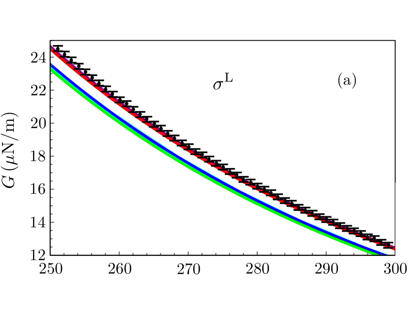
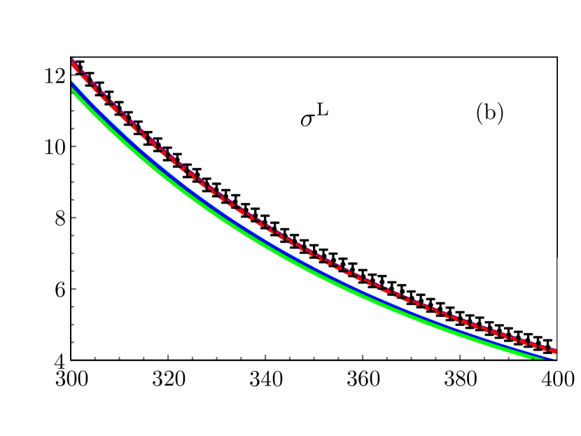
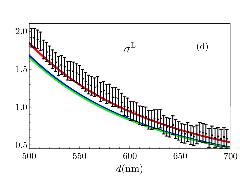
Figure 12: Same as for Fig. 4, where instead of $\sigma^{\rm{K}}$ we use here the Local Kubo conductivity model for graphene $\sigma^{\rm{L}}$ using Eq. (24) and Eq. (22) to obtain the finite $T$ results.

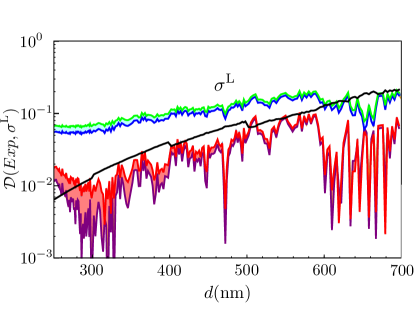
Figure 13: Same as for Fig. 5, where instead of $\sigma^{\rm{K}}$ we use here the Local Kubo conductivity model for graphene $\sigma^{\rm{L}}$ using Eq. (24) and Eq. (22) to obtain the finite $T$ results. Theoretical values below this black curve show cases when the theoretical results are inside the experimental error-bars. We can observe a small discrepancy at short distances.

B.2 Comparison of the experiment with the NR model

By using the NR model [20][13][14] in the CLF gradient $G(d)$ we find the results of figure Fig. 14 and Fig. 15. We can see the same agreement with the experiments as obtained using the non-local Kubo model shown in Fig. 4 and Fig. 5.

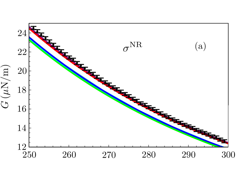
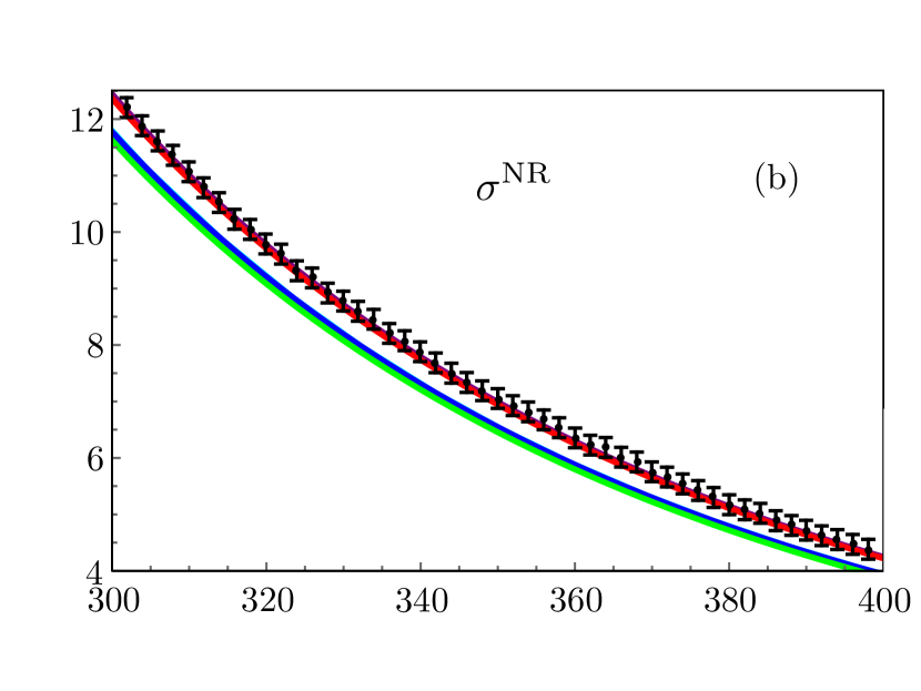
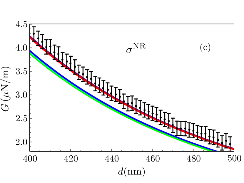
Figure 14: Same as for Fig. 4, where instead of $\sigma^{\rm{K}}$ we use here the the NR conductivity $\sigma^{\rm{NR}}$ of Eq. (23) [20][13][14].

Figure 15: Same as for Fig. 5, where instead of $\sigma^{\rm{K}}$ we use here the the NR conductivity model for graphene $\sigma^{\rm{NR}}$ of Eq. (23) [20][13][14]. Theoretical values below this black curve show cases when the theoretical results are inside the experimental error-bars. We can observe a small discrepancy at short distances.

References

- Dzyaloshinskii et al. [1961] I. E. Dzyaloshinskii, E. M. Lifshitz, and L. P. Pitaevskii, Soviet Physics Uspekhi 4, 153 (1961).
- Abbas et al. [2017] C. Abbas, B. Guizal, and M. Antezza, Phys. Rev. Lett. 118, 126101 (2017).
- Rodriguez-Lopez et al. [2017] P. Rodriguez-Lopez, W. J. M. Kort-Kamp, D. A. R. Dalvit, and L. M. Woods, Nature Communications 8, 14699 (2017).
- Gómez-Santos [2009] G. Gómez-Santos, Phys. Rev. B 80, 245424 (2009).
- Bimonte et al. [2017] G. Bimonte, G. L. Klimchitskaya, and V. M. Mostepanenko, Phys. Rev. B 96, 115430 (2017).
- Bordag et al. [2009a] M. Bordag, I. V. Fialkovsky, D. M. Gitman, and D. V. Vassilevich, Phys. Rev. B 80, 245406 (2009a).
- Drosdoff and Woods [2010] D. Drosdoff and L. M. Woods, Phys. Rev. B 82, 155459 (2010).
- Wang and Antezza [2024] J.-S. Wang and M. Antezza, Phys. Rev. B 109, 125105 (2024).
- Rodriguez-Lopez et al. [2024] P. Rodriguez-Lopez, D.-N. Le, I. V. Bondarev, M. Antezza, and L. M. Woods, Phys. Rev. B 109, 035422 (2024).
- Jeyar et al. [2023a] Y. Jeyar, M. Luo, K. Austry, B. Guizal, Y. Zheng, H. B. Chan, and M. Antezza, Phys. Rev. A 108, 062811 (2023a).
- Jeyar et al. [2023b] Y. Jeyar, K. Austry, M. Luo, B. Guizal, H. B. Chan, and M. Antezza, Phys. Rev. B 108, 115412 (2023b).
- Jeyar et al. [2024] Y. Jeyar, M. Luo, B. Guizal, , H. B. Chan, and M. Antezza, Casimir-lifshitz force for graphene-covered gratings (2024), arXiv:2405.14523 [cond-mat.mes-hall] .
- Liu et al. [2021] M. Liu, Y. Zhang, G. L. Klimchitskaya, V. M. Mostepanenko, and U. Mohideen, Phys. Rev. Lett. 126, 206802 (2021).
- Rodriguez-Lopez and Antezza [2024] P. Rodriguez-Lopez and M. Antezza, Graphene conductivity: Kubo model versus qft-based model (2024), arXiv:2403.02279 [cond-mat.mes-hall] .
- Falkovsky and Pershoguba [2007] L. A. Falkovsky and S. S. Pershoguba, Phys. Rev. B 76, 153410 (2007).
- Bordag et al. [2009b] M. Bordag, G. Klimchitskaya, U. Mohideen, and V. Mostepanenko, Advances in the Casimir Effect, International Series of Monographs on Physics (OUP Oxford, 2009).
- Rodriguez-Lopez et al. [2020] P. Rodriguez-Lopez, A. Popescu, I. Fialkovsky, N. Khusnutdinov, and L. M. Woods, Communications Materials 1, 14 (2020).
- Kubo [1957] R. Kubo, Journal of the Physical Society of Japan 12, 570 (1957), https://doi.org/10.1143/JPSJ.12.570 .
- Rodriguez-Lopez et al. [2018] P. Rodriguez-Lopez, W. J. M. Kort-Kamp, D. A. R. Dalvit, and L. M. Woods, Phys. Rev. Mater. 2, 014003 (2018).
- Bordag et al. [2015] M. Bordag, G. L. Klimchitskaya, V. M. Mostepanenko, and V. M. Petrov, Phys. Rev. D 91, 045037 (2015).
- Zeitlin [1995] V. Zeitlin, Physics Letters B 352, 422 (1995).
- Fialkovsky et al. [2011] I. V. Fialkovsky, V. N. Marachevsky, and D. V. Vassilevich, Phys. Rev. B 84, 035446 (2011).
- Dorey and Mavromatos [1992] N. Dorey and N. Mavromatos, Nuclear Physics B 386, 614 (1992).
- Luttinger [1968] J. M. Luttinger, Transport theory, in Mathematical Methods in Solid State and Superfluid Theory: Scottish Universities’ Summer School, edited by R. C. Clark and G. H. Derrick (Springer US, Boston, MA, 1968) pp. 157–193.
- Rammer [2007] J. Rammer, Quantum Field Theory of Non-equilibrium States (Cambridge University Press, 2007).
- Das Sarma et al. [2011] S. Das Sarma, S. Adam, E. H. Hwang, and E. Rossi, Rev. Mod. Phys. 83, 407 (2011).
- Jablan et al. [2009] M. Jablan, H. Buljan, and M. Soljačić, Phys. Rev. B 80, 245435 (2009).
- Giuliani and Vignale [2005] G. Giuliani and G. Vignale, Quantum Theory of the Electron Liquid (Cambridge University Press, 2005).
- Maldague [1978] P. F. Maldague, Surface Science 73, 296 (1978).
- Palik and Prucha [1997] E. D. Palik and E. J. Prucha, Handbook of optical constants of solids (Academic Press, Boston, MA, 1997).
- Svetovoy et al. [2008] V. B. Svetovoy, P. J. van Zwol, G. Palasantzas, and J. T. M. De Hosson, Phys. Rev. B 77, 035439 (2008).
- Fialkovsky and Vassilevich [2012] I. V. Fialkovsky and D. V. Vassilevich, International Journal of Modern Physics A 27, 1260007 (2012), https://doi.org/10.1142/S0217751X1260007X .
- Klimchitskaya and Mostepanenko [2016] G. L. Klimchitskaya and V. M. Mostepanenko, Phys. Rev. B 93, 245419 (2016).
- Ludwig et al. [1994] A. W. W. Ludwig, M. P. A. Fisher, R. Shankar, and G. Grinstein, Phys. Rev. B 50, 7526 (1994).
- Gusynin et al. [2006] V. P. Gusynin, S. G. Sharapov, and J. P. Carbotte, Phys. Rev. Lett. 96, 256802 (2006).
- Falkovsky and Varlamov [2007] L. A. Falkovsky and A. A. Varlamov, The European Physical Journal B 56, 281 (2007).
- Falkovsky [2008] L. A. Falkovsky, Journal of Experimental and Theoretical Physics 106, 575 (2008).
- Sinitsyn et al. [2006] N. A. Sinitsyn, J. E. Hill, H. Min, J. Sinova, and A. H. MacDonald, Phys. Rev. Lett. 97, 106804 (2006).
- Klimchitskaya and Mostepanenko [2018] G. L. Klimchitskaya and V. M. Mostepanenko, Phys. Rev. D 97, 085001 (2018).
- Xiao and Wen [2013] X. Xiao and W. Wen, Phys. Rev. B 88, 045442 (2013).
- Tse and MacDonald [2010] W.-K. Tse and A. H. MacDonald, Phys. Rev. Lett. 105, 057401 (2010).
- Bimonte [2010] G. Bimonte, Phys. Rev. A 81, 062501 (2010).
- Adam et al. [2007] S. Adam, E. H. Hwang, V. M. Galitski, and S. D. Sarma, Proceedings of the National Academy of Sciences 104, 18392 (2007), https://www.pnas.org/doi/pdf/10.1073/pnas.0704772104 .
- Abrikosov et al. [1975] A. A. Abrikosov, I. Dzyaloshinskii, L. P. Gorkov, and R. A. Silverman, Methods of quantum field theory in statistical physics (Dover, New York, NY, 1975).
- Szunyogh and Weinberger [1999] L. Szunyogh and P. Weinberger, Journal of Physics: Condensed Matter 11, 10451 (1999).
- Yanagisawa and Shibata [2004] T. Yanagisawa and H. Shibata, Optical properties of unconventional superconductors (2004), arXiv:cond-mat/0408054 .
- Bimonte et al. [2016] G. Bimonte, D. López, and R. S. Decca, Phys. Rev. B 93, 184434 (2016).
- Bimonte et al. [2021] G. Bimonte, B. Spreng, P. A. Maia Neto, G.-L. Ingold, G. L. Klimchitskaya, V. M. Mostepanenko, and R. S. Decca, Universe 7, 10.3390/universe7040093 (2021).
- Klimchitskaya and Mostepanenko [2022] G. L. Klimchitskaya and V. M. Mostepanenko, International Journal of Modern Physics A 37, 10.1142/s0217751x22410020 (2022).
- Sushkov et al. [2011] A. O. Sushkov, W. J. Kim, D. A. R. Dalvit, and S. K. Lamoreaux, Nature Physics 7, 230–233 (2011).
- Zhu et al. [2021] T. Zhu, M. Antezza, and J.-S. Wang, Phys. Rev. B 103, 125421 (2021).
- Wang et al. [2021] M. Wang, L. Tang, C. Y. Ng, R. Messina, B. Guizal, J. A. Crosse, M. Antezza, C. T. Chan, and H. B. Chan, Nature Communications 12, 600 (2021).