Tracking controllability for finite-dimensional linear systems

Abstract.

We introduce and analyze the concept of tracking controllability, where the objective is for the state of a control system, or some projection thereof, to follow a given trajectory within a specified time horizon. By leveraging duality, we characterize tracking controllability through a non-standard observability inequality for the adjoint system. This characterization facilitates the development of a systematic approach for constructing controls with minimal norm. However, achieving such an observability property is challenging. To address this, we utilize the classical Brunovský canonical form for control systems, specifically focusing on the case of scalar controls. Our findings reveal that tracking control inherently involves a loss of regularity in the controls. This phenomenon is highly sensitive to the system’s structure and the interaction between the projection to be tracked and the system.

1. Introduction, problem formulation and main results

Let us consider the following classical finite-dimensional linear system:

$$\begin{cases}x^{\prime}(t)=Ax(t)+Bu(t)&t\in(0,T),\\ x(0)=x_{0},\end{cases}$$ (1.1)

where $T>0$, $x:[0,T]\to\mathbb{R}^{n}$ represents the state, $u:[0,T]\to\mathbb{R}^{m}$ denotes the control function with $1\leq m\leq n$, $x_{0}\in\mathbb{R}^{n}$ is the initial condition, and $A\in\mathbb{R}^{n\times n}$ and $B\in\mathbb{R}^{n\times m}$ are time-independent matrices.

The classical concept of “state controllability” refers to the property that, for a given time horizon $T>0$, initial data $x_{0}$, and final state $x_{1}$, there exists a control function $u=u(t)\in L^{2}(0,T;\mathbb{R}^{m})$ such that the unique solution $x=x(t)\in C([0,T];\mathbb{R}^{n})$ of (1.1) satisfies $x(T)=x_{1}$. This property can be characterised through the classical Kalman rank condition, [7]:

$$\text{rank}\Big{[}A\ A^{2}B\ \ldots\ A^{n-1}B\Big{]}=n.$$ (1.2)

We will denote by $K(A,B)$ the extended Kalman matrix $\Big{[}A\ A^{2}B\ \ldots\ A^{n-1}B\Big{]}$.

In this work, inspired by the articles [9], [13] and [1] where the sidewise or tracking control for the wave and heat equations was considered, we introduce and analyze the notion of “tracking controllability” for the finite-dimensional system above.

Definition 1.1.

Let $T>0$ and $E\in\mathbb{R}^{p\times n}$ be the output matrix, for some $p\in\{1,\ldots,n\}$. System (1.1) is said to be $E$-tracking controllable if for any output target $f\in H^{1}(0,T;\mathbb{R}^{p})$ and initial conditions $x_{0}\in\mathbb{R}^{n}$, under the compatibility condition $f(0)=Ex_{0}$, there exists a control function $u\in L^{2}(0,T;\mathbb{R}^{m})$ such that the solution $x\in C([0,T];\mathbb{R}^{n})$ of (1.1) satisfies

$$Ex(t)=f(t),\quad\forall t\in[0,T].$$ (1.3)

When such a control $u\in L^{2}(0,T;\mathbb{R}^{m})$ exists the output target function $f$ is said to be $E$-reachable or $E$-trackable.

Remark 1.2.

Several remarks are in order:

• This new concept of controllability is more general and differs from the classical problem of exact controllability to trajectories. Unlike state controllability, which allows the system’s state to exactly follow a predetermined trajectory, our approach aims to track an arbitrary target function $f=f(t)$, not necessarily a trajectory of the controlled system itself (1.1). This is a demanding condition due to the limitations imposed by the system’s dynamics on its solution trajectories.

• The problem under consideration differs from the state-to-output control property introduced in [2]. System (1.1) is state-to-output controllable, if for any $x_{0}\in\mathbb{R}^{n}$ and $y_{1}\in\mathbb{R}^{p}$, $p\in\{1,\ldots,n\}$, there exists a time $T>0$ and a control $u$ such that the output $y(t)=Cx(t)+Du(t)$ satisfies $y(T)=y_{1}$, where $C\in\mathbb{R}^{p\times n}$ and $D\in\mathbb{R}^{p\times m}$. We refer to [6] for a comprehensive analysis of this type of controllability property. In contrast, our tracking control problem focuses on the entire trajectory over the interval $(0,T)$, not just the output at the final time $t=T$.

• We impose $H^{1}$-regularity on the trajectory $f=f(t)$ to be tracked, in contrast with the $L^{2}$-regularity of the control $u=u(t)$. This is due to intrinsic regularising properties of the system: $L^{2}(0,T)$ regularity of the control $u=u(t)$ implies the $H^{1}(0,T)$ regularity of the solution state $x=x(t)$ and, accordingly, of any of its projections $Ex(t)$. However, as analyzed through the Brunovský canonical form, the $H^{1}$ regularity of the trajectory to be tracked does not suffice, necessitating further regularity assumptions depending on the interactions between the matrices $A,B$ and $E$.

• Due to the linearity of the system, it is sufficient to consider the case where $x_{0}=0$ under the compatibility condition $f(0)=0$.

• Tracking controllability refers to the range of the control-to-output state operator, defined as

  $$\Lambda_{E}:L^{2}(0,T;\mathbb{R}^{m})\to H^{1}(0,T;\mathbb{R}^{p})$$

  $$\Lambda_{E}u(t)=\int_{0}^{t}Ee^{A(t-s)}Bu(s)ds,$$ (1.4)

  which maps into the infinite-dimensional space $H^{1}(0,T;\mathbb{R}^{p})$. This contrasts with the control-to-final state operator $\Gamma:L^{2}(0,T;\mathbb{R}^{m})\to\mathbb{R}^{n}$, defined by

  $$\Gamma u(t)=\int_{0}^{T}e^{A(T-s)}Bu(s)ds,$$

  which maps to $\mathbb{R}^{n}$.

  The infinite-dimensional nature of the range of the control-to-output state operator $\Lambda_{E}$ above introduces significant challenges that we address in this paper.

The main results of this paper are as follows:

• In Section 2, Theorem 2.1, we establish the characterization of the tracking controllability condition for linear systems (1.1) using the control-to-output state operator $\Lambda_{E}$ defined in (• ‣ 1.2) and the corresponding tracking Gramian operator (see (2.2) below). The important differences with respect to the classical state controllability problem will be discussed.

• Further on, in Section 3 we will adapt the classical Hilbert Uniqueness Method (HUM) in order to characterize the minimum norm control for the tracking control property, which is the content of Theorem 3.2. The corresponding adjoint minimization problem is defined on an infinite-dimensional Hilbert space $H^{-1}(0,T;\mathbb{R}^{p})$, with the associated adjoint system having source terms in $H^{-1}(0,T;\mathbb{R}^{p})$. This reflects the important differences with classical controllability problems.

• The approximate control version of tracking controllability will also be analyzed, which allows to avoid, at least in a first approach to the problem, the issues related to the regularity of the tracking target. This will lead to a non-standard unique continuation problem for the adjoint system.

• Our next main contribution, developed in Section 4, will be the analysis of tracking controllability for scalar controls $(m=1)$, with controls $u\in L^{2}(0,T;\mathbb{R})$ and an output matrix $E\in\mathbb{R}^{1\times n}$. Assuming that the system is state controllable, using the famous Brunovský canonical form (see [4]), which we will recall for the sake of completeness and clarity, we establish the tracking controllability of the system in Theorem 4.3.

  The tracking control will be built explicitly and this will allow us to develop a sharp analysis of regularity issues. As we shall see, in some cases the target $f=f(t)$ will need to belong to $H^{n}(0,T;\mathbb{R})$ to assure its tracking with controls in $L^{2}(0,T;\mathbb{R})$.

• In Section 6, we analyze the finite-dimensional models derived from the numerical discretization of wave and heat equations. Later, in Section 7, we present a non-exhaustive list of open problems related to our work, which we hope will lead to interesting developments in the future.

2. Tracking controllability: first results

As mentioned above, in the sequel, without loss of generality, we assume that $x_{0}=0$ and the function $f=f(t)$ will be assumed to satisfy the compatibility conditions $f(0)=0$. Then, the unique solution of (1.1) is given by

$$x(t)=\int_{0}^{t}e^{A(t-s)}Bu(s)ds.$$ (2.1)

Let $f\in H^{1}(0,T;\mathbb{R}^{p})$, $f(0)=0$, be a target function. Then, tracking controllability reduces to finding a control $u=u(t)$ such that

$$f(t)=\int_{0}^{t}Ee^{A(t-s)}Bu(s)ds.$$

The above identity motivates us to define the operator $\Lambda:L^{2}(0,T;\mathbb{R}^{m})\to H_{0}^{1}(0,T;\mathbb{R}^{p})$ as

$$\Lambda_{E}u(t)=\int_{0}^{t}Ee^{A(t-s)}Bu(s)ds.$$

Here and in what follows in this article, we will denote by $H_{0}^{m}(0,T;\mathbb{R}^{k})$, $k\in\mathbb{N}$, the space

$$H_{0}^{m}(0,T;\mathbb{R}^{k}):=\{h\in H^{m}(0,T;\mathbb{R}^{k}):\\ \ h^{(i)}(0)=0,\ i=0,1,\ldots,m-1\}.$$

Note that, in contrast with classical notations for Sobolev spaces, no trace conditions are imposed at $t=T$.

The tracking controllability condition is equivalent to the subjectivity of the operator $\Lambda_{E}$. Let us characterize this condition through its adjoint operator $\Lambda_{E}^{*}:H^{-1}(0,T;\mathbb{R}^{p})\to L^{2}(0,T;\mathbb{R}^{m})$:

$$\langle\psi,\Lambda_{E}u\rangle_{-1,1}=\langle\Lambda_{E}^{*}\psi,u\rangle_{L^{2}(0,T;\mathbb{R}^{m})},$$

for every $\psi\in H^{-1}(0,T;\mathbb{R}^{p}),\ u\in L^{2}(0,T;\mathbb{R}^{m})$. Here, $H^{-1}(0,T;\mathbb{R}^{p})$ stands for the dual of $H_{0}^{1}(0,T;\mathbb{R}^{p})$ which differs from the classical $H^{-1}(0,T;\mathbb{R}^{p})$ space, given that the elements in $H_{0}^{1}(0,T;\mathbb{R}^{p})$ may have a non-trivial trace at $t=T$. Furthermore, $\langle\cdot,\cdot\rangle_{-1,1}$ denotes the duality product between $H^{-1}(0,T;\mathbb{R}^{p})$ and $H_{0}^{1}(0,T;\mathbb{R}^{p})$, with respect to the pivot space $L^{2}(0,T;\mathbb{R}^{p})$.

Using the definition of the inner product in $L^{2}(0,T;\mathbb{R}^{k})$, $k\in\mathbb{N}$, given by

$$\langle\xi,\phi\rangle_{L^{2}(0,T;\mathbb{R}^{k})}=\int_{0}^{T}\xi(t)^{*}\phi(t)dt,\quad\forall\xi,\phi\in L^{2}(0,T;\mathbb{R}^{k}),$$

we have

$$\langle\psi,\Lambda_{E}u\rangle_{-1,1}=\int_{0}^{T}\psi^{*}(t)\left(\int_{0}^{t}Ee^{A(t-s)}Bu(s)ds\right)dt=\int_{0}^{T}\int_{0}^{t}\left(B^{*}e^{A^{*}(t-s)}E^{*}\psi(t)\right)^{*}u(s)dsdt.$$

Then, applying Fubini’s theorem, we get

$$\langle\psi,\Lambda_{E}u\rangle_{-1,1}=\int_{0}^{T}\left(\int_{s}^{T}B^{*}e^{A^{*}(t-s)}E^{*}\psi(t)dt\right)^{*}u(s)ds.$$

Namely, the adjoint operator $\Lambda_{E}^{*}$ of $\Lambda_{E}$ is given by

$$\Lambda_{E}^{*}\psi(t)=\int_{t}^{T}B^{*}e^{A^{*}(\tau-t)}E^{*}\psi(\tau)d\tau,$$

for every $\psi\in H^{-1}(0,T;\mathbb{R}^{p})$. Thus, tracking controllability is effectively equivalent to proving that $\Lambda_{E}^{*}$ is bounded by below, in a sense to be specified (see Theorem 2.1 below).

Moreover, note that

$$(\Lambda_{E}\circ\Lambda_{E}^{*})\psi(t) =\Lambda_{E}\left(\int_{t}^{T}B^{*}e^{A^{*}(\tau-t)}E^{*}\psi(\tau)d\tau\right)=\int_{0}^{t}Ee^{A(t-s)}B\left(\int_{s}^{T}B^{*}e^{A^{*}(\tau-s)}E^{*}\psi(\tau)d\tau\right)ds$$

$$=\int_{0}^{t}\left(\int_{s}^{T}Ee^{A(t-s)}BB^{*}e^{A^{*}(\tau-s)}E^{*}\psi(\tau)d\tau\right)ds.$$

This motivates us to define the tracking Gramian operator $G_{E}:H^{-1}(0,T;\mathbb{R}^{p})\to H_{0}^{1}(0,T;\mathbb{R}^{p})$ as follows

$$G_{E}\psi(t)=\int_{0}^{t}\left(\int_{s}^{T}Ee^{A(t-s)}BB^{*}e^{A^{*}(\tau-s)}E^{*}\psi(\tau)d\tau\right)ds,$$ (2.2)

which, contrarily to classical control problems, takes time-dependent values and will allow us to characterize tracking controllability.

The following characterization of the tracking controllability property holds.

Theorem 2.1.

The following assertions are all equivalent:

1. The system (1.1) is $E$-tracking controllable in the sense of Definition 1.1.

2. The operator $\Lambda_{E}:L^{2}(0,T;\mathbb{R}^{m})\to H_{0}^{1}(0,T;\mathbb{R}^{p})$, defined by

   $$\Lambda_{E}u(t)=\int_{0}^{t}Ee^{A(t-s)}Bu(s)ds,$$

   is surjective.

3. There exists a constant $C>0$ such that the operator $\Lambda_{E}^{*}:H^{-1}(0,T;\mathbb{R}^{p})\to L^{2}(0,T;\mathbb{R}^{m})$ given by

   $$\Lambda_{E}^{*}\psi(t)=\int_{t}^{T}B^{*}e^{A^{*}(\tau-t)}E^{*}\psi(\tau)d\tau,$$

   satisfies

   $$\|\psi\|_{H^{-1}(0,T;\mathbb{R}^{p})}\leq C\|\Lambda_{E}^{*}\psi\|_{L^{2}(0,T;\mathbb{R}^{m})},$$ (2.3)

   for every $\psi\in H^{-1}(0,T;\mathbb{R}^{p})$.

4. The tracking Gramian operator
   $G_{E}:H^{-1}(0,T;\mathbb{R}^{p})\to H_{0}^{1}(0,T;\mathbb{R}^{p})$ defined by

   $$G_{E}\psi(t)=\int_{0}^{t}\left(\int_{s}^{T}Ee^{A(t-s)}BB^{*}e^{A^{*}(\tau-s)}E^{*}\psi(\tau)d\tau\right)ds$$

   is invertible with continuous inverse.

We end this section with some comments.

Remark 2.2.

As described in the Introduction, tracking controllability differs significantly with respect to classical controllability notions. The tracking controllability changes drastically the functional setting, namely the Gramian matrix and the control-to-state operator take values in infinite-dimensional spaces. In this new scenario we no longer have a Gramian matrix, but rather a Gramian operator and the control-to-output state operator is now an operator between infinite-dimensional spaces. Therefore, even in the context of ordinary differential equations, the notion of tracking controllability is an infinite dimensional concept.

3. Tracking observability

Adapting the so-called Hilbert Uniqueness Method (HUM) ([8], [11]) the tracking control problem can be transformed into an observability one for the adjoint system. Doing this is the object of this section.

3.1. $E$-tracking observability

We start by introducing the adjoint system and the notion of solution by transposition. Let $g\in H^{-1}(0,T;\mathbb{R}^{p})$ and $\varphi\in L^{2}(0,T;\mathbb{R}^{n})$ be the unique weak solution in the sense of transposition of the adjoint problem

$$\begin{cases}-\varphi^{\prime}(t)=A^{*}\varphi(t)+E^{*}g(t)&t\in(0,T),\\ \varphi(T)=0.\end{cases}$$ (3.1)

Namely, $\varphi\in L^{2}(0,T;\mathbb{R}^{n})$ is characterised by the weak formulation:

$$\int_{0}^{T}\langle\varphi(t),\phi^{\prime}(t)\rangle_{\mathbb{R}^{n}}dt=\int_{0}^{T}\langle\varphi(t),A\phi(t)\rangle_{\mathbb{R}^{n}}dt+\langle E^{*}g,\phi\rangle_{-1,1},\quad\forall\phi\in H_{0}^{1}(0,T;\mathbb{R}^{n}).$$ (3.2)

We introduce the concept of tracking observability for the adjoint system.

Definition 3.1.

The system (3.1) is said to be tracking observable, if there exists a constant $C>0$ such that

$$\|g\|_{H^{-1}(0,T;\mathbb{R}^{p})}^{2}\leq C\|B^{*}\varphi\|_{L^{2}(0,T;\mathbb{R}^{m})}^{2}\\ =C\left\|\int_{t}^{T}B^{*}e^{A^{*}(s-t)}E^{*}g(s)ds\right\|_{L^{2}(0,T;\mathbb{R}^{m})}^{2},$$ (3.3)

for every $g\in H^{-1}(0,T;\mathbb{R}^{n})$ and $\varphi$ the unique weak solution by transposition of (3.1). We refer to (3.3) as the tracking observability inequality.

With this tracking observability, we are able to prove our second main result.

Theorem 3.2.

Let $A\in\mathbb{R}^{n\times n}$ and $B\in\mathbb{R}^{n\times m}$ be the matrices defining system (1.1), and let $E\in\mathbb{R}^{p\times n}$, $p\in\{1,\ldots,n\}$, be the output matrix. Suppose that the adjoint system (3.1) is tracking observable in the sense of (3.3). Then, for very $f\in H_{0}^{1}(0,T;\mathbb{R}^{p})$ the system (1.1) is $E$-tracking controllable.

Proof.

We proceed in several steps.

• First, using $x=x(t)$ solution of (1.1) with $x(0)=0$ as test function in (3.2), we get

  $$\langle E^{*}g,x\rangle_{-1,1}=\int_{0}^{T}\langle B^{*}\varphi(t),u(t)\rangle_{\mathbb{R}^{m}}dt.$$

  Therefore, the tracking controllability condition $Ex(t)=f(t)$ is equivalent to the following identity

  $$\langle g,f\rangle_{-1,1}=\int_{0}^{T}\langle B^{*}\varphi(t),u(t)\rangle_{\mathbb{R}^{m}}dt,$$ (3.4)

  for every $g\in H^{-1}(0,T;\mathbb{R}^{p})$ and $\varphi\in L^{2}(0,T;\mathbb{R}^{n})$ solution of (3.1).

• Secondly, we observe that (3.4) can be seen as the Euler-Lagrange equation of the critical points when minimizing the quadratic functional

  $$J(g):=\frac{1}{2}\int_{0}^{T}|B^{*}\varphi(t)|^{2}dt-\langle g,f\rangle_{-1,1}$$ (3.5)

  defined for $g\in H^{-1}(0,T;\mathbb{R}^{p})$. Indeed, we have

  $$J(\widehat{g}+hg)-J(\widehat{g}) =\frac{1}{2}\int_{0}^{T}|B^{*}(\widehat{\varphi}(t)+h\varphi(t))|^{2}dt-\langle\widehat{g}+hg,f\rangle_{-1,1}-\frac{1}{2}\int_{0}^{T}|B^{*}\widehat{\varphi}(t)|^{2}dt+\langle\widehat{g},f\rangle_{-1,1}$$

  $$=h\int_{0}^{T}\langle B^{*}\widehat{\varphi}(t),B^{*}\varphi(t)\rangle_{\mathbb{R}^{m}}dt+\frac{h^{2}}{2}\int_{0}^{T}|B^{*}\varphi(t)|^{2}dt-h\langle g,f\rangle_{-1,1}$$

  and the Gateaux derivative takes the form

  $$0=\lim_{t\to 0}\frac{J(\widehat{\varphi}_{1}+h\varphi_{1})-J(\widehat{\varphi}_{1})}{h}=\int_{0}^{T}\langle B^{*}\widehat{\varphi}(t),B^{*}\varphi(t)\rangle_{\mathbb{R}^{m}}dt-\langle g,f\rangle_{-1,1}.$$

  Therefore, if $\widehat{g}$ is the minimiser of $J$, $u(t)=B^{*}\widehat{\varphi}(t)$, where $\widehat{\varphi}$ is the adjont solution of (3.1), corresponding to the minimising source $\widehat{g}$, is the tracking control of minimal $L^{2}$-norm for (1.1).

• Thus, it suffices to prove that functional $J$ defined by (3.5) attains its minimum. The functional $J$ is convex and continuous in $H^{-1}(0,T;\mathbb{R}^{p})$. From the Direct Method of the Calculus of Variations, it suffices to show that $J$ is coercive, that is,

  $$\lim_{\|g\|_{H^{-1}(0,T;\mathbb{R}^{p})}\to\infty}J(g)=\infty.$$

  This coercivity property is an immediate consequence of the tracking observability inequality (3.3). Indeed,

  $$J(g)=\frac{1}{2}\int_{0}^{T}|B^{*}\varphi(t)|^{2}dt-\langle g,f\rangle_{-1,1}\geq\frac{C}{2}\|g\|_{H^{-1}(0,T;\mathbb{R}^{p})}^{2}-\|g\|_{H^{-1}(0,T;\mathbb{R}^{p})}\|f\|_{H_{0}^{1}(0,T;\mathbb{R}^{p})}.$$

∎

Remark 3.3.

Note that, unlike in classical control theory for ordinary differential equations, the following unique continuation property for the solution of the adjoint system is insufficient to achieve tracking observability/controllability:

$$B^{*}\varphi(t)=0\ \forall t\in[0,T]\ \text{ implies }\ g\equiv 0.$$ (3.6)

Indeed, while the observability inequality immediately implies this unique continuation property, the converse is not true, due to the infinite-dimensionality of the problem. By the contrary, in the finite-dimensional state control context the equivalence of these concepts stems from the equivalence of norms in finite-dimensional spaces. This phenomenon is analogous to the classical context of controllability of infinite-dimensional Partial Differential Equations (PDE) problems, where the unique continuation property does not suffice to obtain quantitative observability inequalities.

Actually, as we shall see below, there exist finite-dimensional systems $(A,B)$ and output operators $E$ for which the unique continuation property holds, but the observability inequality as stated above is not fulfilled. Instead, only a weaker version of the observability inequality, involving a loss of a finite number of Sobolev derivatives, is satisfied.

3.2. Approximate $E$-tracking controllability

Motivated by the previous remark and the intrinsic infinite-dimensional character of the observability inequality under consideration, we introduce the notion of approximate tracking controllable system.

Definition 3.4.

Let $T>0$ and $E\in\mathbb{R}^{p\times n}$ be the output matrix. We will say that system (1.1) is approximately $E$-tracking controllable if for any output target $f\in L^{2}(0,T;\mathbb{R}^{p})$, $p\in\{1,\ldots,n\}$, and for every $\varepsilon>0$, there exists a control function $u\in L^{2}(0,T;\mathbb{R}^{m})$ such that the solution $x\in C([0,T];\mathbb{R}^{n})$ of (1.1) satisfies

$$\|Ex(t)-f(t)\|_{L^{2}(0,T;\mathbb{R}^{p})}\leq\varepsilon.$$ (3.7)

Note that approximate tracking controllability is formulated in the $L^{2}(0,T;\mathbb{R}^{p})$-setting, for the sake of simplicity. Of course, as it is classical in the context of infinite-dimensional systems, approximate controllability is a much weaker control property, since it does not provide neither further information about the actual reachable targets and their regularity, nor any quantitative information on the size of the controls needed to assure the $\varepsilon$ proximity property.

The following dual characterization assures that it is equivalent to the unique continuation property mentioned above:

Theorem 3.5.

System (1.1) is approximately $E$-tracking controllable if and only if the adjoint system (3.1) satisfies the unique continuation property (3.6).

Proof.

We proceed in several steps.

• Step 1. Existence of the minimiser.

  Let us assume first that the unique continuation property (3.6) holds.

  Approximate controls can be obtained through the minimisation of the functional $J_{\epsilon}:L^{2}(0,T;\mathbb{R}^{p})\to\mathbb{R}$ given by

  $$J_{\epsilon}(g):=\frac{1}{2}\int_{0}^{T}|B^{*}\varphi(t)|^{2}dt-\langle g,f\rangle_{L^{2}(0,T;\mathbb{R}^{p})}+\varepsilon\|g\|_{L^{2}(0,T;\mathbb{R}^{p})}.$$

  It is immediate that $J_{\epsilon}$ is a continuous and convex functional.

  It is by now classical now the unique contribution property also ensures the coervicity of $J_{\epsilon}$. Indeed, let $\{g_{k}\}_{k\geq 1}\subset L^{2}(0,T;\mathbb{R}^{p})\setminus\{0\}$ be a sequence of source terms for the adjoint system (3.1) such that $\|g_{k}\|_{L^{2}(0,T;\mathbb{R}^{p})}\to\infty$ as $k\to\infty$. Let $\varphi_{k}$ be the corresponding solutions of (3.1) and $\widetilde{\varphi}_{k}\in C([0,T];\mathbb{R}^{n})$ be the normalised ones, with source term $\widetilde{g}_{k}=g_{k}/\|g_{k}\|_{L^{2}(0,T;\mathbb{R}^{p})}$. Then,

  $$\frac{J(g_{k})}{\|g_{k}\|_{L^{2}(0,T;\mathbb{R}^{p})}}=\frac{1}{2}\|g_{k}\|_{L^{2}(0,T;\mathbb{R}^{p})}\int_{0}^{T}|B^{*}\widetilde{\varphi_{k}}(t)|^{2}dt+\varepsilon-\langle\widetilde{g}_{k},f\rangle_{L^{2}(0,T;\mathbb{R}^{p})}.$$ (3.8)

  We observe that if

  $$\liminf_{k\to\infty}\int_{0}^{T}|B^{*}\widetilde{\varphi}(t)|^{2}dt>0,$$

  then the coercivity of the functional $J_{\epsilon}$ is immediately obtained. Therefore, let us consider the most delicate situation where we assume that $\int_{0}^{T}|B^{*}\widetilde{\varphi_{k}}(t)|^{2}dt\to 0$.

  Extracting subsequences we have $\widetilde{g}_{k_{j}}\rightharpoonup h$ weakly in $L^{2}(0,T;\mathbb{R}^{p})$ and the corresponding solutions satisfy $\widetilde{\varphi}_{k_{j}}\rightharpoonup\eta$ weakly in $H^{1}(0,T;\mathbb{R}^{p})$, where $\eta\in C([0,T];\mathbb{R}^{n})$ is the unique solution of

  $$\begin{cases}-\eta^{\prime}(t)=A^{*}\eta(t)+E^{*}h(t)&t\in(0,T),\\ \eta(T)=0.\end{cases}$$

  We also have

  $$\int_{0}^{T}|B^{*}\eta(t)|^{2}dt\leq\liminf_{j\to\infty}\int_{0}^{T}|B^{*}\widetilde{\varphi}_{k_{j}}(t)|^{2}dt=0.$$

  That is, $B^{*}\eta=0$ for every $t\in(0,T)$. By (3.6) we deduce that $h\equiv 0$. Accordingly, $\widetilde{g}_{k_{j}}\rightharpoonup 0$ and then $\langle\widetilde{g}_{k_{j}},f\rangle_{L^{2}(0,T;\mathbb{R}^{p})}\to 0$, as $j\to\infty$. From (3.8), we obtain

  $$\liminf_{j\to\infty}\frac{J(g_{k_{j}})}{\|g_{k_{j}}\|_{L^{2}(0,T;\mathbb{R}^{p})}}\geq\varepsilon$$

  which implies

  $$\lim_{\|g_{k}\|_{L^{2}(0,T;\mathbb{R}^{p})}\to\infty}J(g_{k})=\infty$$

  and the coercivity of $J$.

  Now, since the functional $J$ is continuous, convex and coercive, there exists $\overline{g}\in L^{2}(0,T;\mathbb{R}^{p})$ such that $J(\overline{g})=\min_{g\in L^{2}(0,T;\mathbb{R}^{p})}J(g)$.

• Step 2. Euler-Lagrange equations.

  The minimiser fulfils

  $$0 \leq J(\overline{g}+\delta g)-J(\overline{g})$$

  $$=\delta\int_{0}^{T}\langle B^{*}\overline{\varphi}(t),B^{*}\varphi(t)\rangle_{\mathbb{R}^{m}}dt+\frac{\delta^{2}}{2}\int_{0}^{T}|B^{*}\varphi(t)|^{2}dt-\delta\langle g,f\rangle_{L^{2}(0,T;\mathbb{R}^{p})}+\varepsilon|\delta|\|g\|_{L^{2}(0,T;\mathbb{R}^{p})},$$

  for every $g\in L^{2}(0,T;\mathbb{R}^{p})$, $\overline{\varphi}$ and $\varphi$ being the solutions of (3.1) associated to the optimal solution $\overline{g}$ and $g$, respectively.

  Dividing by $\delta$ and taking limit when $\delta\to 0^{+}$ and $\delta\to 0^{-}$, we obtain

  $$\left|\int_{0}^{T}\Big{(}\langle B^{*}\overline{\varphi}(t),B^{*}\varphi(t)\rangle_{\mathbb{R}^{m}}-\langle g(t),f(t)\rangle_{\mathbb{R}^{p}}\Big{)}dt\right|\leq\varepsilon\|g\|_{L^{2}(0,T;\mathbb{R}^{p})}.$$ (3.9)

  Taking $u=B^{*}\overline{\varphi}$ as a control in (1.1), multiplying (1.1) by $\varphi$ and integrating by parts we get

  $$\int_{0}^{T}\langle x(t),E^{*}g(t)\rangle_{\mathbb{R}^{n}}dt=\int_{0}^{T}\langle B^{*}\overline{\varphi}(t),B^{*}\varphi(t)\rangle_{\mathbb{R}^{m}}dt.$$ (3.10)

  Therefore, replacing this into (3.9), we finally obtain

  $$\left|\int_{0}^{T}\langle Ex(t)-f(t),g(t)\rangle_{\mathbb{R}^{p}}dt\right|\leq\varepsilon\|g\|_{L^{2}(0,T;\mathbb{R}^{p})},$$

  that is, the approximate tracking controllability property (3.7) holds.

• Step 3. Reciprocally, assume that system (1.1) is approximate tracking controllable and let $g\in L^{2}(0,T;\mathbb{R}^{p})\setminus\{0\}$ be such that $B^{*}\varphi(t)=0$ for every $t\in[0,T]$. Our aim is to show that, then, $g\equiv 0$. Given that $B^{*}\varphi(t)=0$, multiplying the controlled system by $\varphi$ and integrating by parts we get that

  $$\int_{0}^{T}\langle Ex(t),g(t)\rangle_{\mathbb{R}^{p}}dt=0,$$

  for every control $u\in L^{2}(0,T;\mathbb{R}^{m})$. However, given that the system fulfills the property of approximate controllability, it follows that the subspace of the projected trajectories of the form $Ex(t)$ is dense in $L^{2}(0,T;\mathbb{R}^{p})$. This implies that $g\equiv 0$.

∎

The following remarks are in order.

Remark 3.6.

• According to Theorem 3.5, the approximate tracking controllability property reduces to the unique continuation property (3.6). Note, however, that this is a non-standard unique continuation property that does not fit within the classical theory of Cauchy problems and requires an in-depth analysis that we will address in the sequel.

• As it occurs in the PDE setting for classical control problems, even when the unique continuation property (3.6) holds and consequently the approximate controllability is fulfilled, this property yields very little information about the actual class of controllable data, which, in the present case, refers to the targets that can be tracked. This issue also requires an in-depth analysis.

4. Tracking controllability: the scalar control case

In this section, we present a case where tracking controllability holds as a consequence of the state controllability of the system, explicitly obtaining the tracking control function.

We begin with some classical preliminaries.

First, it is important to mention that when the matrices $A$ and $B$ do not satisfy the Kalman rank condition (see (1.2)), that is, if $\text{rank}K(A,B)=r<n$, there exists an invertible matrix $T\in\mathbb{R}^{n\times n}$ such that

$$T^{-1}AT=\left[\begin{array}[]{cc}A_{1}&A_{2}\\ 0&A_{3}\end{array}\right],\quad T^{-1}B=\left[\begin{array}[]{c}B_{1}\\ 0\end{array}\right],$$ (4.1)

where $A_{1}\in\mathbb{R}^{r\times r}$, $B_{1}\in\mathbb{R}^{r\times m}$, and $(A_{1},B_{1})$ is controllable (see, for instance, [10, Lemma 3.3.3]). This classical result is known as the Kalman decomposition into the controllable and non-controllable components of the state.

The second one, based on the Kalman decomposition, is the classification of linear controllable systems given by Brunovský [4]. In order to introduce them, let us recall the definition of similar control system.

Definition 4.1.

The linear control systems $x_{1}^{\prime}=A_{1}x_{1}+B_{1}u_{1}$ and $x_{2}^{\prime}=A_{2}x_{2}+B_{2}u_{2}$ are said to be similar if there exists a nonsingular matrix $P\in\mathbb{R}^{n\times n}$ such that $A_{2}=PA_{1}P^{-1}$ and $B_{2}=PB_{1}$.

We now focus on the scalar control case $m=1$, so that $B$ is just a column vector $B=b$. The classical result by Brunovský on the canonical form of a control system assures that if $(A,b)$ is controllable, then there exists a similar system in the sense of Definition 4.1 with a very particular and easy to handle structure.

Theorem 4.2 ([4]).

Let $A\in\mathbb{R}^{n\times n}$ be given. If $b\in\mathbb{R}^{n}$ such that $(A,b)$ is controllable, then there exist an invertible matrix $P\in\mathbb{R}^{n\times n}$ such that $(A,b)$ is similar to $(\widetilde{A},\widetilde{B})$, where

$$A=P\widetilde{A}P^{-1}\quad\text{and}\quad b=P\widetilde{B}.$$ (4.2)

Here $\widetilde{B}=e_{n}$ is the canonical vector in $\mathbb{R}^{n}$ and the matrix $\widetilde{A}$ is the companion matrix given by

$$\widetilde{A}=\left[\begin{array}[]{ccccc}0&1&0&\ldots&0\\ 0&0&1&\ldots&\vdots\\ \vdots&\vdots&\ddots&\ddots&0\\ 0&0&0&\ldots&1\\ -\alpha_{n}&-\alpha_{n-1}&\ldots&\ldots&-\alpha_{1}\end{array}\right],$$ (4.3)

where $\{\alpha_{1},\ldots,\alpha_{n}\}$ are the coefficients of the characteristic polynomial of $A$. The columns $\{p_{1},\ldots,p_{n}\}$ of the matrix $P$ are given explicitly by

$$p_{k}=\begin{cases}b,&k=n,\\ \displaystyle\left(A^{n-k}+\sum_{j=1}^{n-1}\alpha_{j}A^{n-k-j}\right)b,&1\leq k\leq n-1.\end{cases}$$ (4.4)

Conversely, if there exists an invertible matrix $P\in\mathbb{R}^{n\times n}$ such that $A=P\widetilde{A}P^{-1}$, then $(A,b)$, with $b=Pe_{n}$, is controllable.

Using the Brunovský canonical form we are able to state and prove our next main result, which roughly speaking, ensures that every controllable system with scalar control is also tracking controllable, but under suitable regularity assumptions on target functions.

Theorem 4.3.

Let $A\in\mathbb{R}^{n\times n}$ and $b\in\mathbb{R}^{n}$ be given and such that system (1.1) is $(A,b)$-controllable. Let $E\in\mathbb{R}^{1\times n}$ be the output vector. Then, there exists $k^{*}\in\{1,\ldots,n\}$ such that for every scalar output target $f\in H_{0}^{n-k^{*}+1}(0,T;\mathbb{R})$, there exists a scalar control $u\in L^{2}(0,T;\mathbb{R})$ such that $\langle E,x(t)\rangle_{\mathbb{R}^{n}}=f(t)$, for very $t\in[0,T]$.

Before we get into the proof the following remarks are in order:

Remark 4.4.

• One of the most interesting aspects of this result is the regularity needed on the target to guarantee the tracking controllability property, namely, $H_{0}^{n-k^{*}+1}(0,T;\mathbb{R})$. The precise value of $k^{*}$ needed to determine this regularity class emerges naturally in the proof, as we shall see.

• The state controllability assumption in Theorem 4.3 allows the use of Brunovský’s Theorem 4.2. In the absence of the state controllability property, one could expect to apply the same ideas to the controllable component of the system. The above result could also be extended to the non-scalar case using the general Brunovský canonical form given by

  $$\widetilde{A}=\left[\begin{array}[]{cccc}\widetilde{A}_{1}&0&\ldots&0\\ 0&\widetilde{A}_{2}&\ldots&0\\ \vdots&\vdots&\ddots&\vdots\\ 0&0&\ldots&\widetilde{A}_{s}\end{array}\right],$$ (4.5)

  where each $\widetilde{A}_{i}$, $i=1,\ldots,s$, is a companion matrix and

  $$\widetilde{B}G=\left[\begin{array}[]{c}\widetilde{B}_{1}\\ \vdots\\ \widetilde{B}_{2}\end{array}\right],$$ (4.6)

  for some matrix $G\in\mathbb{R}^{m\times s}$, where all the coefficients of each matrix $\widetilde{B}_{i}$, $i=1,\ldots,s$, except for the one in last row and the $i$-th column, which is equal to $1$.

Proof.

Let assume that system (1.1) is $(A,b)$-controllable and let $f\in L^{2}(0,T;\mathbb{R})$ be a scalar output target. According to Theorem 4.2, there exists a non singular matrix $P\in\mathbb{R}^{n\times n}$ such that $(A,b)$ is similar to $(\widetilde{A},\widetilde{B})$, where $\widetilde{A}$ is the companion matrix given by (4.3) and $\widetilde{B}=e_{n}$, with $e_{n}\in\mathbb{R}^{n}$ the vector $e_{n}=(0,0,\ldots,0,1)$. Namely, we can rewrite system (1.1) as

$$\begin{cases}y^{\prime}(t)=\widetilde{A}y+e_{n}u(t),&t\in(0,T),\\ y(0)=0,\end{cases}$$ (4.7)

where $x=Py$ and $P$ is given by (4.4).

Given that the output matrix belongs to $\mathbb{R}^{1\times n}$, that is, $E=(\xi_{1},\ldots,\xi_{n})$, with $\xi_{i}\in\mathbb{R}$ for $i\in\{1,\ldots,n\}$, the tracking controllability property reads

$$f(t)=\sum_{k=1}^{n}\xi_{k}x_{k}(t).$$

Using the matrix $P$, the tracking control property on the new state $y$ of (4.7) can be written as $\widetilde{E}y(t)=EPy(t)=f(t)$ with $\widetilde{E}=EP$ and, in view of the definition of the matrix $P$ (see (4.4)), as

$$\langle\widetilde{E},y(t)\rangle_{\mathbb{R}^{n}}=\langle E,p_{1}\rangle_{\mathbb{R}^{n}}y_{1}(t)+\ldots+\langle E,p_{n}\rangle_{\mathbb{R}^{n}}y_{n}(t)\\ =f(t),\quad\forall t\in[0,T],$$ (4.8)

with $y(t)=(y_{1}(t),\ldots,y_{n}(t))$. All in all, the tracking controllability for system (4.7) reduces to finding a scalar control $u$ such that

$$f(t)=\sum_{j=1}^{n}\eta_{i}y_{i}(t),\quad\forall t\in[0,T],$$ (4.9)

with $\eta_{i}=\langle E,p_{i}\rangle_{\mathbb{R}^{n}}$, for $i=1,\ldots,n$.

Let $k^{*}\in\{1,\ldots,n\}$ now be the index characterized by the condition

$$\max_{k}\{\eta_{k}\}\neq 0.$$ (4.10)

We rewrite (4.9) as

$$\eta_{k^{*}}y_{k^{*}}(t)=f(t)-\sum_{j=1}^{k^{*}-1}\eta_{j}y_{j}(t).$$ (4.11)

From the definition of the companion matrix $\widetilde{A}$, and more specifically its $(k^{*}-1)$-th row, we get

$$y_{k^{*}-1}^{\prime}(t)=y_{k^{*}}(t)=\frac{1}{\eta_{k^{*}}}\left(f(t)-\sum_{j=1}^{k^{*}-1}\eta_{j}y_{j}(t)\right),$$

and then

$$y_{k^{*}-1}^{\prime}(t)+\frac{\eta_{k^{*}-1}}{\eta_{k^{*}}}y_{k^{*}-1}(t)=\frac{1}{\eta_{k^{*}}}\left(f(t)-\sum_{j=1}^{k^{*}-2}\eta_{j}y_{j}(t)\right).$$

Now, using that $y_{k^{*}-2}^{\prime}(t)=y_{k^{*}-1}$, we obtain

$$y_{k^{*}-2}^{\prime\prime}(t)+\frac{\eta_{k^{*}-1}}{\eta_{k^{*}}}y_{k^{*}-2}^{\prime}(t)+\frac{\eta_{k^{*}-2}}{\eta_{k^{*}}}y_{k^{*}-2}(t)=\frac{1}{\eta_{k^{*}}}\left(f(t)-\sum_{j=1}^{k^{*}-3}\eta_{j}y_{j}(t)\right).$$

Following the previous procedure, the first component of $y$ can be determined by solving the following ordinary differential equation of order $(k^{*}-1)$:

$$\begin{cases}\displaystyle y_{1}^{(k^{*}-1)}(t)+\frac{1}{\eta_{k^{*}}}\sum_{j=1}^{k^{*}-1}\eta_{j}y_{1}^{(j-1)}=\frac{1}{\eta_{k^{*}}}f(t),&t\in(0,T),\vspace*{0.2cm}\\ y_{1}(0)=\ldots=y_{1}^{(k^{*}-2)}(0)=0.\end{cases}$$

Note that the solution of the previous ODE depends only on $f$ and the coefficients $\eta_{i}$, $i=1,\ldots,k^{*}$.

Once this solution has been obtained, the structure of the canonical form allows to compute in cascade all the components of the vector function $y(t)$ up to the index $k^{*}$. They depend only on $f$ and the coefficients $\eta_{i}$, $i=1,\ldots,k^{*}$.

Using again the structure of the companion matrix, we have:

$$y_{k^{*}+1}(t)=y_{k^{*}}^{\prime}(t)=\frac{1}{\eta_{k^{*}}}\left(f^{\prime}(t)-\sum_{j=1}^{k^{*}-1}\eta_{j}y_{j}^{\prime}(t)\right),$$

up to the penultimate term, which reads,

$$y_{n-1}^{\prime}(t)=y_{n}(t)=\frac{1}{\eta_{k^{*}}}\left(f^{(n-k^{*})}(t)-\sum_{j=1}^{k^{*}-1}\eta_{j}y_{j}^{(n-k^{*})}(t)\right).$$

Furthermore, from the last row of the matrix $\widetilde{A}$, we get

$$y_{n}(t)+\alpha_{1}y_{n}(t)=u(t)-\sum_{j=1}^{n-1}\alpha_{n+j-1}y_{j}(t),$$

which leads to the expression of the needed control

$$u(t)=\frac{1}{\eta_{k^{*}}}\left(f^{(n-k^{*}+1)}(t)-\sum_{j=1}^{k^{*}-1}\eta_{j}y_{j}^{(n-k^{*}+1)}(t)\right)+\frac{\alpha_{1}}{\eta_{k^{*}}}\left(f^{(n-k^{*})}(t)-\sum_{j=1}^{k^{*}-1}\eta_{j}y_{j}^{(n-k^{*})}(t)\right)\\ +\sum_{j=1}^{n-1}\alpha_{n+j-1}y_{j}(t).$$ (4.12)

We conclude the existence of a control $u\in L^{2}(0,T;\mathbb{R})$, given by (4.12), such that the solution of (1.1) satisfies $\langle E,x(t)\rangle_{\mathbb{R}^{n}}=f(t)$, for every $t\in[0,T]$. This concludes the proof. ∎∎

In light of this proof, the following comments are warranted:

Remark 4.5.

• We have considered the case where the output is a scalar. Similar methods allow considering more general cases.

  Let us consider, for instance, a simple example, where the output matrix $\widetilde{E}$ has two components instead of one in the canonical form of the system: $\widetilde{E}y(t)=(y_{1}(t),y_{2}(t))^{*}=(f(t),g(t))^{*}$. We impose the natural compatibility conditions on the targets, that is $f(0)=g(0)=0$. The canonical form of the system, ensures $y_{1}^{\prime}(t)=y_{2}(t)$, and this imposes a second compatibility condition

  $$f^{\prime}(t)=g(t)\quad\text{or}\quad f(t)=\int_{0}^{t}g(\tau)d\tau.$$

  Under this condition the method of proof of Theorem 4.3, allows to build the needed control. We omit the details for brevity.

  However, it is important to emphasize that, when considering output operators $E\in\mathbb{R}^{p\times n}$ with multiple outputs $p\geq 2$, tracking controllability imposes compatibility conditions on the vector valued target functions.

  The condition $\max_{k}\{\eta_{k}\}\neq 0$ in the proof of Theorem 4.3, which gives us the critical index $k^{*}$, determines the necessary regularity needed for the target, namely, $H_{0}^{n-k^{*}+1}(0,T;\mathbb{R})$. Let us show with a simple example how this condition appears in practice.

  We consider the output matrix $\widetilde{E}y(t)=y_{1}(t)+y_{2}(t)=f(t)$. The first compatibility condition is $f(0)=0$. Using that $y_{2}(t)=f(t)-y_{1}(t)$ and by the definition of the companion matrix $\widetilde{A}$, we get

  $$y_{1}^{\prime}(t)=f(t)-y_{1}(t).$$

  And by Leibniz formula,

  $$y_{1}(t)=\int_{0}^{t}e^{-(t-s)}f(s)ds.$$

  Using once more time the companion matrix, the following explicit formula for the control is obtained

  $$u(t)=\displaystyle f^{(n-1)}(t)-\sum_{k=0}^{n-2}f^{(k)}(t)-y_{1}(t)+\alpha_{1}\left(f^{(n-2)}(t)-\sum_{k=0}^{n-3}f^{(k)}(t)+y_{1}(t)\right)\\ -\sum_{j=1}^{n-1}\alpha_{n+j-1}\left(\sum_{i=0}^{j-2}f^{(i)}(t)+y_{1}(t)\right).$$

  In this case $k^{*}=2$ and $H_{0}^{n-1}(0,T;\mathbb{R})$ is the needed regularity condition on the target function for the control to belong to $L^{2}(0,T;\mathbb{R})$.

5. Numerical examples

In this part of the article, we develop some numerical examples to validate our findings. For that, we will numerically solve the following optimal control problem

$$\min_{u}J(u)=\frac{1}{2}\int_{0}^{T}|u(t)|^{2}dt+\frac{\alpha}{2}\int_{0}^{T}|Ex(t)-f(t)|^{2}dt$$ (5.1)

subject to $x$ solves the systems

$$\begin{cases}x^{\prime}(t)=Ax(t)+Bu(t)&t\in(0,T),\\ x(0)=x_{0},\end{cases}$$ (5.2)

The cost function $J$ includes a term that penalizes the difference between the state $Ex$ and the desired trajectory $f$. That is, this is the penalized version (see, for instance, [3]) of the classical HUM approach which consists in finding the control with minimal $L^{2}$-norm. The penalty is weighted by a factor $\alpha$, which can be adjusted to give more or less weight to the tracking error compared to the control effort. The $\alpha$ parameter determines the relative weight of tracking error in the cost function. A higher value of $\alpha$ will give more importance to accurate tracking of the desired trajectory, while a lower value will give more importance to minimizing the control effort. This approach allows us to control the trade-off between minimizing control effort and tracking the desired trajectory more flexibly. In all the examples we fixed this parameter in $\alpha=10^{4}$.

Let us fix a time horizon $T=10$ and we introduce our first system

$$A=\left(\begin{array}[]{cc}0&1\\ -2&-3\end{array}\right),\ B=\left(\begin{array}[]{c}0\\ 1\end{array}\right).$$

We denote by $x=x(t)=(x_{1}(t),x_{2}(t))$ the state and by $u=u(t)$ the scalar control acting in the second component of the system. We set the initial condition $x_{0}=(1,1)$. In this case, the free solution, that is $u\equiv 0$, is plot in Figure 1.

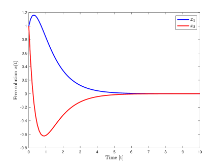
Figure 1. This plot depicts the state $x=(x_{1},x_{2})$ of the system without any control input over time. It serves as a baseline to compare the performance of the control strategy.

.

We compute the optimal pair $(u^{T},x^{T})$ of problem (5.1)-(5.2) by using CasADi open-source tool for nonlinear optimization and algorithmic differentiation. Specifically, we solve the optimal control problem with the IPOPT solver.

In our first numerical example, we consider the following output matrix $E=(1\ 0)$ and the output target $f(t)=\sin\left(\frac{1}{2}t+\frac{\pi}{2}\right)$. Let us observe that $f(0)=1=Ex(0)$. The Mean Squared Error (MSE) between the reference and output is $0.0002$. The result is plotted in Figure 2. We note that the control allows us to obtain the desired tracking control.

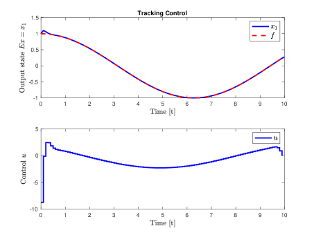
Figure 2. This plot shows the state $x_{1}$ of the system (blue line) and the desired tracking path $f$ (red dashed line) over time. The objective is for $Ex=x_{1}$ to follow the reference path $f$ as closely as possible. Also illustrates the optimal control input $u$ over time, which is computed to minimize the cost function and ensure that the system state tracks the desired path.

In the case we track the second component of the solution $E=(0\ 1)$, the MSE is $5.83e-06$ and the results are contained in Figure 3. Obviously, in the present case since the control function is in the second component of the state, we obtain better result than in the previous case.

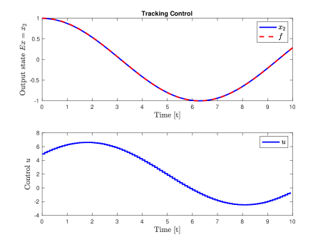
Figure 3. This plot shows the state $x_{2}$ of the system (blue line) and the desired tracking path $f$ (red dashed line) over time. The control is now smoother than in the previous case.

Different is the situation, as we have discussed in previous sections, when the output target function is not regular enough. For instance, in Figure 4 we can observe the case when $E=(1\ 0)$ and $f(t)=[t+1]$, where $[\cdot]$ denotes the floor function (or greatest integer function). The MSE in this case is $0.0178$.

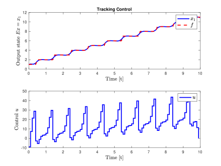
Figure 4. This plot shows the state $x_{1}$ of the system (blue line) and the desired tracking path $f$ not regular enough (red dashed line) over time. In addition, illustrates the optimal control input $u$ over time, which is computed to minimize the cost function and ensure that the system state tracks the desired path.

The last numerical example is for the semidiscrete heat equation with interior control. Namely, we analysis numerically the penalized HUM approach to solve

$$\min_{u}J(u)=\frac{\beta}{2}\int_{0}^{T}\int_{0}^{1}|u(x,t)|^{2}dxdt+\frac{\alpha}{2}\int_{0}^{T}|y_{x}(1,t)-f(t)|^{2}dt$$

subject to $y=y(x,t)$ solves the heat equation

$$\begin{cases}y_{t}-y_{xx}=u&(x,t)\in(0,1)\times(0,T),\\ y(0,t)=y(1,t)=0&t\in(0,T),\\ y(x,0)=0&x\in(0,1),\end{cases}$$

where here we consider a sufficiently regular target function $f(t)=\sin(2\pi t)$.

The following illustrates the application of the open-source tool CasADi to solve the optimal control problem for the heat equation .The scenario involves a rod of length $L=1$ over a time horizon $T=1$, discretized into $Nx=100$ spatial points and $Nt=200$ temporal points. The penalization parameters $\beta$ and $\alpha$ are set to $1\times 10^{-3}$ and $1\times 10^{3}$, respectively, emphasizing the tracking objective.

The state equations are discretized using the Crank-Nicolson scheme. Boundary conditions are enforced at both ends of the rod, with the left end fixed at zero temperature and the right end’s normal derivative matching $f(t)$. The constraints and objective function are formulated within the CasADi framework and solved using the Ipopt solver. The solution includes the optimal state and control variables.

Using the open-source tool CasADi, we find the optimal pair $(u^{T},y^{T})$. Since in this case the tracking controllability is related to the normal derivative, Figure 5 shows that the penalized optimal control problem successfully solves the desired problem. Specifically, the control function effectively modifies the state so that the normal derivative at the right end of the interval follows the given trajectory. In this case, the mean squared error (MSE) is $0.00054873$.

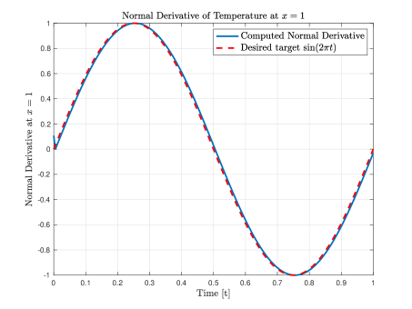
Figure 5. This figure shows the normal derivative of the temperature $y_{x}$ of the system at $x=1$ (blue line) and the desired tracking path $f$ regular enough (red dashed line) over time.

6. Examples: Semi-discrete wave and heat equations

As seen previously, the results of this paper are applicable to general linear finite-dimensional systems, including their application to the numerical discretization of PDE models. This section is devoted to a brief discussion of the finite-difference discretization of one-dimensional wave and heat equations.

Let us first consider the following $1-d$ wave equation with control at the left hand side of the interval $(0,L)$, that is,

$$\begin{cases}w_{tt}-w_{xx}=0&x\in(0,L),\ t\in(0,T),\\ w(0,t)=u(t),\ w(L,t)=0&t\in(0,T),\\ w(x,0)=w_{0}(x)&x\in(0,L),\\ w_{t}(x,0)=w_{1}(x)&x\in(0,L).\end{cases}$$ (6.1)

The tracking controllability property discussed in this article can also be considered in the PDE context of (6.1). Given a time horizon $T>0$, initial data $w_{0},w_{1}$, and a target $f=f(t)$ for the flux at $x=L$, the objective is to find a control function $u=u(t)$ such that the solution $w(x,t)$ of (6.1) satisfies $w_{x}(L,t)=f(t)$ for every $t\in[0,T]$. The results in [9], [13] provide a positive solution when $T>L$, for target functions in $L^{2}(L,T)$ and with boundary controls $u\in H^{1}(0,T)$. The fact that the time-horizon $T$ needs to satisfy $T>L$ for the tracking controllability to hold is a consequence of the finite velocity of propagation.

Consider now the finite-difference semi-discretization

$$\begin{cases}w_{j}^{\prime\prime}+\frac{2w_{j}-w_{j-1}-w_{j+1}}{h^{2}}=0&j=1,\ldots,M,\quad t\in(0,T),\\ w_{0}=u(t),\quad w_{M+1}=0&t\in(0,T),\\ w_{j}(0)=\varphi_{j},\quad w_{j}^{\prime}(0)=\phi_{j}&j=1,\ldots,M,\end{cases}$$ (6.2)

with $h=\frac{L}{M+1}>0$ with $M\in\mathbb{N}$, defining nodes $x_{j}=jh$ for $j=0,\ldots,M+1$. The initial conditions $(\varphi_{j},\phi_{j})_{j=1}^{M}$ typically approximate the initial data $(w_{0},w_{1})$ of the wave equation (6.1) on the mesh. System (6.2) consists of $M$ coupled second-order differential equations with $M$ unknowns. The state components $w_{1}(t),\ldots,w_{M}(t)$ provide approximations of the solution $w=w(x,t)$ of the wave equation at mesh points $x_{1},\ldots,x_{M}$.

In this context, the tracking controllability can be stated as finding a control $u=u(t)$ such that the solution of the semi-discrete system (6.2) satisfies

$$\frac{w_{M+1}-w_{M}}{h}=f(t),\quad\forall t\in[0,T]$$ (6.3)

since the left hand side term approximates the normal derivative. This tracking condition can be written equivalently as follows:

$$w_{M}=-hf(t),$$ (6.4)

because $w_{M+1}\equiv 0$. The state-controllability of this finite-dimensional system is well known. In fact, the Kalman rank condition is easy to check. Accordingly, the system also fulfills the tracking controllability property.

In fact, for this model the control can be computed explicitly out of the target. Indeed, substituting the tracking condition into the system with (6.2) for $j=M$, we obtain

$$w_{M-1}=-h^{3}p^{\prime\prime}(t)-2hp(t).$$

Repeating this process for $j=M-1$, we find

$$w_{M-2}=-h^{5}p^{(4)}(t)-4h^{3}p^{\prime\prime}(t)-3hp(t),$$

and so forth,

$$w_{M-3}=-h^{7}p^{(6)}(t)-6h^{5}p^{(4)}(t)-10h^{3}p^{\prime\prime}(t)-4hp(t),...$$

This leads to an explicit control function.

Thus, in agreement with the results obtained using Brunovský’s canonical form, the semi-discrete system fulfils the tracking controllability property with $L^{2}$-controls when the target to be tracked is in $H^{2M}(0,T)$. Importantly, in this semi-discrete setting, tracking controllability is achieved without any restrictions on the time horizon.

The same analysis can be done in the context of the heat equation, namely for the system

$$\begin{cases}z_{j}^{\prime}+\frac{2z_{j}-z_{j-1}-z_{j+1}}{h^{2}}=0&j=1,\ldots,M,\ t\in(0,T),\\ z_{0}=u(t),\ z_{M+1}=0&t\in(0,T),\\ z_{j}(0)=\varphi_{j}&j=1,\ldots,M.\end{cases}$$ (6.5)

In this case for the control to be in $L^{2}$ it suffices that the target lies in $H^{M}(0,T)$.

7. Further comments and open problems

In this final section, we present some open problems, perspectives and future research lines.

• We would like to emphasize the distinctions between our work and the existing literature on finite-dimensional control theory. The proof and implications of Theorem 4.3, along with the findings presented in Section 3, show the infinite-dimensional nature of tracking controllability. Much remains to be explored for both finite-dimensional and PDE models. Current understanding of the lateral or tracking controllability properties of wave and heat equations, primarily through energy estimates, microlocal analysis, and transmutation techniques, is still in its nascent stages.

• Moreover, as discussed in the previous section, the use of Brunovský’s canonical form in reformulating the tracking control problem proves highly relevant in the finite-dimensional setting. This approach not only simplifies the construction of explicit tracking controls but also provides valuable insights into the regularity of the target function $f$ necessary to achieve $L^{2}$-controls.

The following is a non-exhaustive list of open problems:

• Semi-discrete wave equation: The wave equation serves as a prototypical example where tracking or sidewise controllability is applicable, as previously explained. Consequently, it is natural to investigate whether tracking controls for numerical approximation schemes converge to the tracking control of the continuous wave equation as the mesh size tends to zero. It is well-documented that in scenarios requiring precise control to drive the solution exactly to a final target, convergent numerical schemes may yield unstable control approximations due to high-frequency spurious numerical solutions [12]. The procedure outlined above to explicitly find the control for the semi-discrete wave equation does shows clearly an unstable behaviour as $h\to 0$, demanding an increasing order of regularity of the target to be reachable as the dimension of the finite-dimensional system increases. It would be interesting to see if the filtering techniques developed in [12] and related works can clarify the limit process and the need of the minimal time $T>L$ at the PDE level.

  Similar questions can be formulated for the heat equation and its finite-dimensional approximations.

• Analytic output target function: In the finite-dimensional context of this paper, tracking controllability is equivalent to satisfying the equation

  $$f(t)=\int_{0}^{t}Ee^{A(t-s)}Bu(s)\,ds.$$ (7.1)

  If $f$ is an analytic function satisfying $f(0)=0$, assuming the control function $u$ is also analytic, and evaluating consecutive derivatives at $t=0$, the equation is equivalent to the following infinite-dimensional system:

  $$f^{\prime}(0) =EBu(0),$$

  $$f^{\prime\prime}(0) =EBu^{\prime}(0)+EABu(0),$$

  $$f^{\prime\prime\prime}(0) =EBu^{\prime\prime}(0)+EABu^{\prime}(0)+EA^{2}Bu(0),$$

  $$\dots$$

  The invertibility of the matrix $EB\in\mathbb{R}^{p\times m}$ is sufficient to compute consecutive derivatives of the control $u$ at $t=0$. Does this procedure lead to a convergent series determining an analytic control function $u(t)$? How is such a result related to Theorem 2.1 above?

• Moment problem formulation: Consider the case where $A$ admits a spectral decomposition. For instance, for a symmetric real matrix $A$ such that $A=A^{*}$ with spectrum $\lambda_{k}$, $Ae_{k}=\lambda_{k}e_{k}$ for all $k\leq n$. Multiplying (2.1) by $e_{k}$, we obtain

  $$\langle x(t),e_{k}\rangle_{\mathbb{R}^{n}}=\int_{0}^{t}e^{\lambda_{k}(t-s)}\langle u(s),B^{*}e_{k}\rangle_{\mathbb{R}^{m}}\,ds.$$

  Utilizing the orthonormality of normalized eigenvectors, we derive

  $$x(t)=\sum_{k}\left(\int_{0}^{t}e^{\lambda_{k}(t-s)}\langle u(s),B^{*}e_{k}\rangle_{\mathbb{R}^{m}}\,ds\right)e_{k}.$$

  The tracking controllability property reduces to

  $$Ex(t)=f(t)=\sum_{k}\left(\int_{0}^{t}e^{\lambda_{k}(t-s)}\langle u(s),B^{*}e_{k}\rangle_{\mathbb{R}^{m}}\,ds\right)Ee_{k}.$$

  Assuming $Ee_{k}$ forms an orthonormal (up to normalization constants) basis of $\mathbb{R}^{p}$, we decompose the target $f(t)$ as

  $$f(t)=\sum_{k}\langle f(t),Ee_{k}\rangle_{\mathbb{R}^{p}}Ee_{k}.$$

  This leads to the integral equations for the control $u=u(t)$:

  $$f_{k}(t)=\int_{0}^{t}e^{\lambda_{k}(t-s)}\langle u(s),B^{*}e_{k}\rangle_{\mathbb{R}^{m}}\,ds,\quad\forall k\leq n,$$ (7.2)

  where $f_{k}(t)=\langle f(t),Ee_{k}\rangle_{\mathbb{R}^{p}}$.

  In the specific case where the control function is scalar, $m=1$, system (7.2) becomes

  $$f_{k}(t)=c_{k}\int_{0}^{t}e^{\lambda_{k}(t-s)}u(s)\,ds,\quad\forall k\leq n,$$

  where $c_{k}:=B^{*}e_{k}\in\mathbb{R}$. Therefore, assuming $c_{k}\neq 0$ for all $k\leq n$, the control problem can be reduced to a type of moment problem: finding a control $u=u(t)\in L^{2}(0,T)$ such that

  $$\frac{f_{k}(t)}{c_{k}}=\int_{0}^{t}e^{\lambda_{k}(t-s)}u(s)\,ds,\quad\forall k\leq n.$$

  Now, with $f\in H_{0}^{1}(0,T;\mathbb{R}^{p})$ and a finite number of distinct eigenvalues $\lambda_{k}$, $k\in\{1,\ldots,N\}$, the tracking control can be explicitly determined by the formula

  $$u(t)=\frac{f_{k}^{\prime}(t)}{c_{k}}-\lambda_{k}\frac{f_{k}(t)}{c_{k}},\quad t\in(0,T),\ k\in\{1,\ldots,N\}.$$ (7.3)

  Hence, to ensure coherence, we impose the following strong compatibility condition on the output target function:

  $$\frac{f_{i}^{\prime}(t)}{c_{i}}-\lambda_{i}\frac{f_{i}(t)}{c_{i}}=\frac{f_{j}^{\prime}(t)}{c_{j}}-\lambda_{j}\frac{f_{j}(t)}{c_{j}},\quad\forall i\neq j.$$

  This represents an initial attempt to formulate a moment problem for tracking controllability, but further analysis is required in both the finite and infinite-dimensional settings.

• Tracking observability inequality: The analysis of the observability inequality presented in (3.3) deserves significant attention and meticulous study. Establishing this inequality within the context of ordinary differential equations may shed light on proving related inequalities, such as those involved in sidewise or tracking controllability for the heat equation, a problem recently proposed in [1]. The application of Carleman inequalities for ordinary differential equations, as demonstrated in [5], could be instrumental in addressing this issue and provide valuable insights into the methodology.

• Simultaneous state and tracking controllability: It is well-established that state controllability can be achieved for a wide range of control functions. Consequently, it is natural to seek controls within this family that also satisfy tracking controllability. This leads to the following problem: identifying controls that simultaneously drive the state to a specified target $x_{1}\in\mathbb{R}^{n}$ and ensure the tracking control property $Ex(t)=f(t)$. In other words, is it possible to achieve both state and tracking controllability simultaneously? Despite the apparent simplicity of this question, addressing it is far from trivial. Refer to [9].

References

- [1] J. A. Barcena-Petisco and E. Zuazua. Tracking controllability for the heat equation. https://arxiv.org/pdf/2310.00314v2, 2024.
- [2] J. Bertram and P. Sarachik. On optimal computer control. IFAC Proceedings Volumes, 1(1):429–432, 1960. 1st International IFAC Congress on Automatic and Remote Control, Moscow, USSR, 1960.
- [3] F. Boyer. On the penalised HUM approach and its applications to the numerical approximation of null-controls for parabolic problems. In CANUM 2012, 41e Congrès National d’Analyse Numérique, volume 41 of ESAIM Proc., pages 15–58. EDP Sci., Les Ulis, 2013.
- [4] P. Brunovský. A classification of linear controllable systems. Kybernetika (Prague), 6:173–188, 1970.
- [5] F. W. Chaves-Silva, L. Rosier, and E. Zuazua. Null controllability of a system of viscoelasticity with a moving control. J. Math. Pures Appl. (9), 101(2):198–222, 2014.
- [6] B. Danhane, J. Lohéac, and M. Jungers. Characterizations of output controllability for LTI systems. Automatica J. IFAC, 154:Paper No. 111104, 10, 2023.
- [7] R. E. Kalman. Contributions to the theory of optimal control. Bol. Soc. Mat. Mexicana (2), 5:102–119, 1960.
- [8] J. L. Lions. Contrôlabilité exacte perturbations et stabilisation de systèmes distribués. Tome 1, Contrôlabilité exacte., volume 8. Recherches en Mathematiques Appliquées, Masson, 1988.
- [9] Y. Saraç and E. Zuazua. Sidewise profile control of 1-D waves. J. Optim. Theory Appl., 193(1-3):931–949, 2022.
- [10] E. D. Sontag. Mathematical control theory, volume 6 of Texts in Applied Mathematics. Springer-Verlag, New York, second edition, 1998. Deterministic finite-dimensional systems.
- [11] E. Zuazua. Some problems and results on the controllability of partial differential equations. In European Congress of Mathematics, pages 276–311. Springer, 1998.
- [12] E. Zuazua. Propagation, observation, and control of waves approximated by finite difference methods. SIAM Rev., 47(2):197–243, 2005.
- [13] E. Zuazua. Fourier series and sidewise control of 1-d waves, volume 22. Documents Mathématiques of the French Mathematical Society (SMF), 2024.