Singularity formation of hydromagnetic waves in cold plasma
Abstract.
We study blow-up of the compressible fluid model introduced by Gardner and Morikawa, which describes the dynamics of a magnetized cold plasma. We propose sufficient conditions that lead to blow-up. In particular, we find that smooth solutions can break down in finite time even if the gradient of initial velocity is identically zero. The density and the gradient of the velocity become unbounded as time approaches the lifespan of the smooth solution. The Lagrangian formulation reduces the singularity formation problem to finding a zero of the associated second-order ODE.
Keywords: Cold plasma; Hydromagnetic waves; Singularities
1. Introduction
Under suitable assumptions, the motion of a magnetized cold plasma can be described by the the following simplified model [7]:
| (1.1a) | |||
| (1.1b) | |||
| (1.1c) | |||
| (1.1d) | |||
where represents the number density of ions, is the -component of the ion velocity, is the difference between the -components of the ion and electron velocities, and is the -component of the magnetic field. All unknowns in (1.1) are functions of . The system (1.1) can be formally derived from the two-species 3D Euler-Maxwell system [6] under the following assumptions: (i) all unknown functions are uniform in the and directions, (ii) the magnetic field is applied only in the direction, (iii) the densities of ions and electrons are the same (quasineutrality), (iv) slow motion (the displacement current is neglected), (v) cold plasma (the pressure effects are neglected), and (vi) (1.1d) holds at .
The system (1.1) was introduced in [7] to investigate hydromagnetic waves propagating across a magnetic field. Despite being one of the first examples from which the KdV equation was derived outside the context of water waves, the system (1.1) has not received much attention. We refer to [5, 8] for studies on the oblique propagation of hydromagnetic waves. In [10], the KdV limit of (1.1) is rigorously justified. The work of [1] formally derives some asymptotic models of (1.1) and investigates their properties. In particular, wave-breaking phenomena (derivative blow-up) can occur in these asymptotic models of (1.1); see [1, 11].
We show that the solution to (1.1) blows up in finite time for a certain class of initial data. Our result is particularly interesting since it implies that the solution may blow up even if the gradient of the initial velocity is identically zero.
1.1. Main result
We consider smooth solutions to (1.1) with the far-field state as . For initial data , the classical solution to the system (1.1) exists locally in time [2]. For given , we see that and are determined by (1.1c)–(1.1d): and . As long as the smooth solution to (1.1) exists, the energy
| (1.2) |
is conserved, i.e., for .
Now, we present our main theorem. Let .
Theorem 1.1.
If the initial data satisfies one of the following:
| (1.3a) | |||
| (1.3b) | |||
| (1.3c) | |||
then the maximal existence time of the classical solution to the system (1.1) is finite. Moreover, and as .
We notice that the condition (1.3a) does not require to have a negative gradient. We illustrate a class of the initial data satisfying and (1.3a). Using the identity (2.1b), we obtain
Hence, it is clear that one can choose the initial data such that and . In particular, one can choose and , where is a standard bump function supported on , with and being sufficiently small.
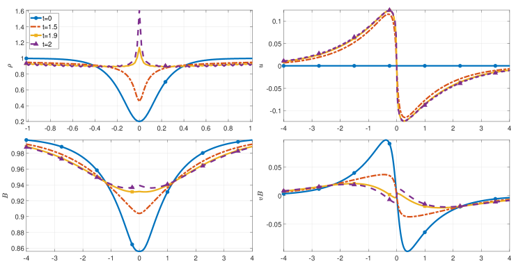
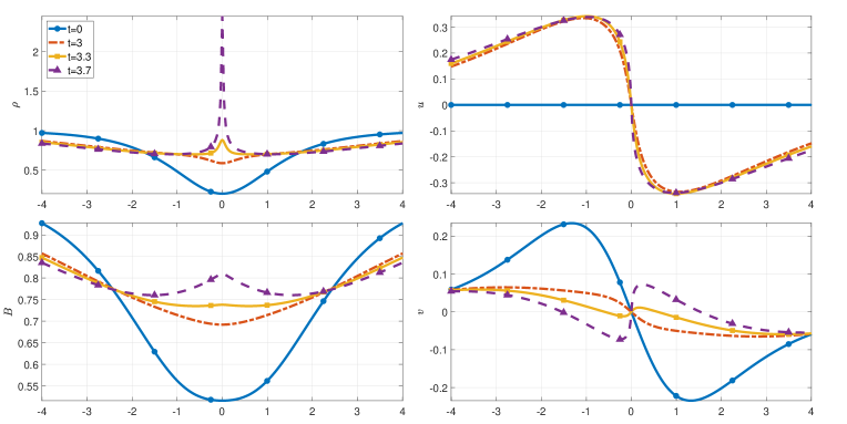
As approaches the blow-up time , diverges since remains uniformly bounded on (see (1.1d) and Lemma 2.1). On the other hand, our numerical simulations show that is also uniformly bounded on (see Figure 1 and 2) resulting in the blow-up of due to (1.1c). We also remark that various simulations suggest that sufficient conditions (1.3) are not optimal (see Figure 2).
The gradient of the velocity blows up due to the hyperbolic part (1.1b) of (1.1). On the other hand, due to the absence of pressure, the system (1.1) is weakly coupled and not hyperbolic, leading to the density blow-up. A natural question arises: what is the asymptotic behavior of solutions near (and at) the blow-up time and location? Specifically, at the blow-up time, (1) whether the density blow-up profile is the so-called delta shock, and (2) whether the blow-up profile for exhibits a jump discontinuity. In fact, the same question was posed in [3] for the pressureless Euler-Poisson system, and it was shown in [4] that, generically, the density is not a Dirac measure and the velocity exhibits regularity at the blow-up time. It would be interesting to investigate more precise structure of singularities in the solutions to (1.1).
To prove Theorem 1.1, we follow the strategy of [3] (see also Appendix 5.5 in [4]), which is two-fold: we derive a second-order ODE using the Lagrangian formulation and establish a uniform (in and ) bound of . More specifically, by defining where is the characteristic curve satisfying , , we derive the initial value problem for the second-order ODE for :
| (1.4) |
where and are evaluated at . If vanishes at some finite time , then the solution to (1.1) blows up in the topology. Hence, it boils down to finding sufficient conditions that guarantee vanishes in finite time.
2. Proof of Theorem 1.1
We first show the key lemma concerning with the uniform estimates for .
Lemma 2.1.
As long as the classical solution to (1.1) exists, it holds that for ,
| (2.1a) | |||
| (2.1b) | |||
Proof.
Now we derive the second-order ODE (1.4). For , let be the solution to the ODE
| (2.5) |
where . Here, we consider the initial position as a parameter. By taking of (2.5), we have
| (2.6) |
where . Integrating (2.6), we get
| (2.7) |
Using (1.1a) and (2.6), one can see that
| (2.8) |
By taking of (1.1b), we have
| (2.9) |
where we have used (1.1c) and (1.1d). Using (2.6), (2.9) and (2.8), we get (1.4). Indeed, we have
From (2.8), we see that since and that
| (2.10) |
Remark 1.
If is (uniformly) bounded as long as the solution exists (or if we have ), one can show that implies . Furthermore, one can also obtain the blow-up rate . We refer to the proof of Lemma 2.3 of [3].
In what follows, we prove Theorem 1.1. We first consider the case (i). For the initial data satisfying (1.3a), we let be the maximal existence time of the solution to (1.1). Then, using (2.1a) for (1.4), we have
| (2.11) |
We let and . Then, (2.11) can be put in the form of , and we have (recalling )
| (2.12) |
where we let for notational simplicity. Since (i.e., (1.3a) holds) and the integrand in (2.12) is nonpositive on , by putting into (2.12), we have . Hence, we conclude that must vanish at some point on the interval by the intermediate value theorem. From (2.10), this implies that the maximal existence time is finite.
Next, we consider the case (ii). Consider the solution to (1.1) with the initial data satisfying (1.3b). Using the trigonometric identity, (2.12) becomes
| (2.13) |
where
Since , . Hence, for , and the cosine function has the minimum value . We recall that the integrand of (2.13) is nonpositive on . Hence, from (2.13), we see that if and (i.e., (1.3b) holds), then vanishes at some point on .
Acknowledgments.
J.B. was supported by the National Research Foundation of Korea grant funded by the Ministry of Science and ICT (2022R1C1C2005658). J.C. was supported by the National Research Foundation of Korea grant funded by the Korean government (MSIT) (2021R1C1C2008763). B.K. was supported by Basic Science Research Program through the National Research Foundation of Korea (NRF) funded by the Ministry of science, ICT and future planning (NRF-2020R1A2C1A01009184).
References
- [1] D. Alonso-Orán, A. Durán, and R. Granero-Belinchón: Derivation and well-posedness for asymptotic models of cold plasmas, Nonlinear Anal., 244 (2024), 113539
- [2] D. Alonso-Orán, R. Granero-Belinchón: Well-posedness for an hyperbolic-hyperbolic-elliptic system describing cold plasmas, Appl. Math. Lett. 147 (2024) 108863
- [3] J. Bae, J. Choi, B. Kwon: Formation of singularities in plasma ion dynamics, Nonlinearity 37 (2024) 045011
- [4] J. Bae, Y. Kim, B. Kwon: Delta-shock for the pressureless Euler-Poisson system, preprint, arXiv:2407.15669
- [5] Y. A. Berezin, V. Karpman: Theory of nonstationary finite-amplitude waves in a low-density plasma, Sov. Phys. JETP 19 1265–1271 (1964).
- [6] F.F. Chen: Introduction to plasma physics and controlled fusion. 2nd edition, Springer (1984)
- [7] C. S. Gardner, G. K. Morikawa: Similarity in the asymptotic behavior of collision-free hydromagnetic waves and water waves. New York Univ., Courant Inst. Math. Sci., Res. Rep. NYO-9082 (1960)
- [8] T. Kakutani, H. Ono, T. Taniuti, C.-C. Wei: Reductive perturbation method in nonlinear wave propagation ii. application to hydromagnetic waves in cold plasma, Journal of the Physical Society of Japan, 24 (5) 1159–1166 (1968).
- [9] Y. Li, D. Sattinger: Soliton Collisions in the Ion Acoustic Plasma Equations. J. math. fluid mech. 1, 117-130 (1999)
- [10] X. Pu, M. Li: Kdv limit of the hydromagnetic waves in cold plasma, Z. Angew. Math. Phys. 70 (1) (2019) 32.
- [11] S. Yang, J. Chen: Wave breaking in the unidirectional non-local wave model, Journal of Differential Equations, Volume 377, 2023, Pages 849-858