“Twist Vectors” for Central Configuration Equations

Abstract.

A new coordinate system on the tangent space to planar configurations is introduced to simplify some calculations on central configurations and relative equilibria in the $N$-body problem with a homogeneous potential, which includes the case of Newtonian gravity. These coordinates are applied to some problems on four-body central configurations to illustrate their utility.

1. Introduction

In this paper we consider the generalization of relative equilibria to ‘central configurations’ for a homogeneous family of potentials that includes the Newtonian case. As the classical Newtonian $N$-body problems do not possess static equilibria, the relative equilibria (equilibria in a uniformly rotating coordinate system) are important anchors from which we can extend our understanding of the dynamics of these systems. We introduce some coordinates on the tangent space of configurations that we believe provides a simplifying context for some known equations and results, and which will hopefully allow further progress.

There is a large literature on central configurations, from which we recommend the book chapter by Moeckel [31] for a wide ranging summary and background.

Most of the natural questions concerning central configurations in the three-body problem have been answered, such as their existence, geometry, and number [13, 22], and their linear stability [15, 38, 37]. However for the four-body and higher $N$-body problems many open questions remain [1], including the most famous problem of the finiteness of planar central configurations [9, 42, 41].

2. Twist Vectors and Central Configurations

We define a (scale-normalized) central configuration by the conditions

(1) $$(q_{i}-c)-\sum_{j=1,j\neq i}^{n}\frac{m_{j}(q_{i}-q_{j})}{r_{i,j}^{A}}=0$$

where $q_{i}\in\mathbf{R}^{d}$ is the position of particle $i$, and $r_{i,j}=|q_{i}-q_{j}|$ are the mutual distances between the particles. $A>2$ is a real parameter. The vector $c$ is the center of mass,

$$c=\frac{1}{M}\sum_{i=1}^{n}m_{i}q_{i},$$

with $M=\sum_{i=1}^{n}m_{i}$ the total mass.

We will focus on the most studied case of planar configurations $(d=2)$. When considering the space of configurations we will use the flattened coordinates in $\mathbf{R}^{2n}$: $(x_{1},y_{1},x_{2},y_{2},\ldots,x_{n},y_{n})$.

An equivalent, sometimes more convenient version of the equations 1 is

(2) $$\sum_{k=1,j\neq i}^{n}m_{k}(q_{i}-q_{k})(r_{i,k}^{-A}-1)=0.$$

These equations can be viewed as critical point equations in several different ways; we choose to consider them as requiring the gradient of $f$ to be zero where

$$f=MI/2+U/(A-2)$$

in which $I=\sum_{i=1}^{n}m_{i}|q_{i}-c|^{2}$ is the moment of inertia around the center of mass, and $U=\sum_{i=1}^{n}m_{i}m_{j}r_{i,j}^{-A+2}$ is a homogeneous potential function. For the special case $A=2$, which is of some interest in the theory of fluid vorticity [19, 21, 4], we can instead use $U=\sum_{i=1}^{n}m_{i}m_{j}\ln(r_{i,j})$ (without the division by $(A-2)$).

At a critical point Euler’s relation for homogeneous functions implies that

$$U=MI.$$

In terms of mutual distances this condition can be written as

$$\sum_{i>j}m_{i}m_{j}r_{i,j}^{2}\left(r_{i,j}^{-A}-1\right)=0.$$

Our choice of definitions means we have set the scale for the overall size of the central configurations; because of the rotational and translation invariance of the Newtonian dynamics the main point of interest is the shape of the central configurations (i.e. modulo uniform rotation and translation). Therefore it is helpful to recast the equations (2) in terms of translation- and rotation-invariant geometric quantities such as the mutual distances $r_{i,j}$. One way to do that is to take the inner product of each (vector-valued) equation in (2) with the difference vector $q_{i}-q_{j}$ for some choice of $j\neq i$:

(3) $$b_{i,j}=\sum_{k=1,k\neq i}^{n}m_{k}(r_{i,k}^{-A}-1)(r_{i,j}^{2}+r_{i,k}^{2}-r_{j,k}^{2})=0,$$

which we call the ‘asymmetric Albouy-Chenciner equations’ (originally coined by Gareth Roberts). When summed in symmetric pairs, $g_{i,j}=b_{i,j}+b_{j,i}$, we obtain the (symmetric) Albouy-Chenciner equations [2, 18].

The fact that the Albouy-Chenciner equations involve only the mutual distances can be both an advantage or disadvantage. For the planar case, once $n>3$ the mutual distances are no longer independent, and it can be a major complicating factor to add in their constraints (e.g. using Cayley-Menger determinants).

We will focus on an alternative, which has been described many times before, sometimes called the Laura-Andoyer equations [23, 3, 26, 16], and extend them to a framework that also includes the Hessian of $f$ in order to exploit Morse theory [29, 8]. Morse theory can be used to obtain lower bounds on the number of central configurations, and the Hessian index is also related to the stability of the central configurations [20, 7, 32, 17].

In order to make our formulas more concise, we will use the notation $x_{i,k}=x_{i}-x_{k}$, $y_{i,j}=y_{i}-y_{j}$, $q_{i,j}=(x_{i,j},y_{i,j})$, $R_{i,k}=r_{i,k}^{-A}$, $S_{i,k}=r_{i,k}^{-A}-1$, $T_{i,k}=r_{i,k}^{-A-2}$, $A_{i,j,k}=r_{i,j}^{2}+r_{i,k}^{2}-r_{j,k}^{2}$, and

$$\Lambda_{i,j,k}=q_{i,j}\wedge q_{i,k}=(x_{i,j}y_{i,k}-x_{i,k}y_{i,j}),$$

which is twice the signed area of the points $q_{i}$, $q_{j}$, and $q_{k}$.

The $\Lambda_{i,j,k}$ change sign under odd permutations of the indices, also note $A_{i,j,k}=A_{i,k,j}$ and $A_{i,j,j}=2r_{i,j}^{2}$.

With this notation the equations (3) become simply

$$b_{i,j}=\sum_{k=1,k\neq i}^{n}m_{k}S_{i,k}A_{i,j,k}=0.$$

Note that in the sum for $b_{i,j}$, the term with $k=j$ plays a somewhat special role, so it can be convenient to separate it out:

$$b_{i,j}=2m_{j}S_{i,j}+\sum_{k\notin\{i,j\}}m_{k}S_{i,k}A_{i,j,k}=0.$$

Our main new tool is to introduce what we will call ‘twist vectors’. These configuration space tangent vectors rotate a pair of points around their center of mass. The nonzero components of the twist vectors at a configuration of points with coordinate $q_{i}=(x_{i},y_{i})$ are

$$\left(v_{i,j}\right)_{x_{i}}=m_{j}y_{i,j},\ \ \ \ \left(v_{i,j}\right)_{y_{i}}=-m_{j}x_{i,j},$$

$$\left(v_{i,j}\right)_{x_{j}}=-m_{i}y_{i,j},\ \ \ \ \left(v_{i,j}\right)_{y_{j}}=m_{i}x_{i,j}.$$

The vectors $v_{i,j}$ are all perpendicular to the vectors $\nabla c_{x}=(m_{1},0,m_{2},0,\ldots,m_{n},0)/M$ and $\nabla c_{y}=(0,m_{1},0,m_{2},\ldots,0,m_{n})/M$, so the orbit of a configuration under the flow generated by any linear combination of the $v_{i,j}$ will have a constant center of mass $c=(c_{x},c_{y})$.

The $v_{i,j}$ are also all tangent to the level surfaces of the moment of inertia, $I$, since $\nabla I=2(m_{1}x_{1},m_{1}y_{1},\ldots,m_{n}x_{n},m_{n}y_{n})$ and thus

$$\nabla I\cdot v_{i,j}=2m_{i}m_{j}(y_{i,j}x_{i}-x_{i,j}y_{i}-y_{i,j}x_{j}+x_{i,j}y_{j})=0.$$

An example of one of these vectors is shown in Figure (1).

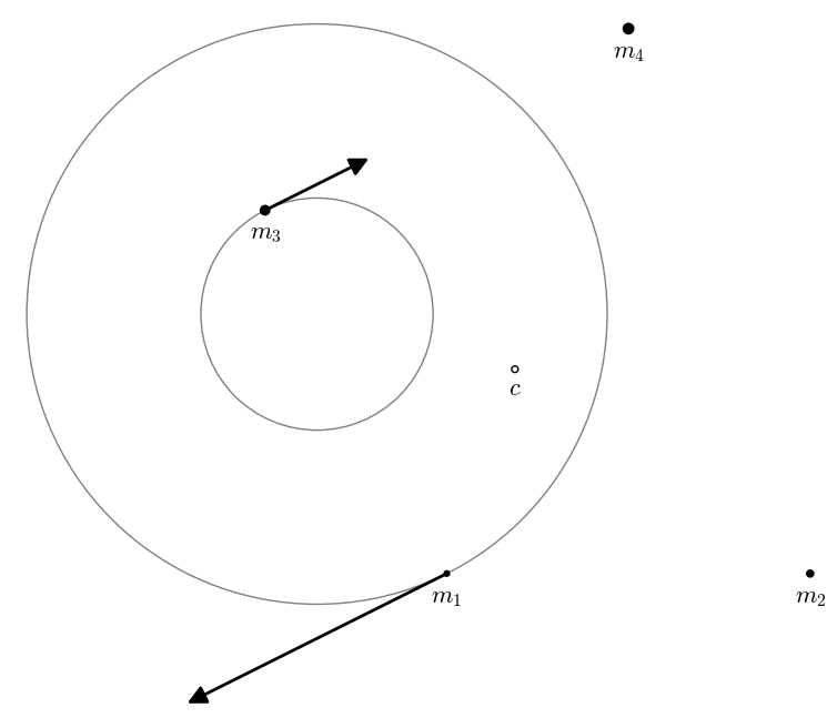
Figure 1. A twist vector $v_{1,3}$ in a configuration of four masses, with $m_{1}=2$, $m_{2}=3$, $m_{3}=5$, and $m_{4}=6$. The system’s center of mass $c$ is shown as an open circle.

Theorem 2.1.

The dimension of the subspace spanned by the (planar) $v_{i,j}$ is $2n-3$, unless all $n$ points are collinear, in which case the dimension is $n-1$.

Proof.

If all $N$ points are collinear, we can pick coordinates so that $x_{i}=0$ for each $1\leq i\leq n$. Then the $y_{i}$ components of the $v_{i,j}$ are all zero, and the $v_{i,j}$ are perpendicular to $\nabla c_{x}$, so the dimension of the span of the $v_{i,j}$ is at most $n-1$. It is easy to see that $v_{1,j}$ are independent for $j>1$, so this subset is a basis for the span.

If the points are not all collinear, assume without loss of generality that $q_{1}$, $q_{2}$, and $q_{3}$ are not collinear. By computing the determinant of the first few 3 by 3 minors of the matrix with rows $v_{1,2}$, $v_{1,3}$, $v_{2,3}$ it can be seen that these three vectors are independent. Now we proceed by induction, assuming that we have a set $S_{k}$ of $2k-3$ independent vectors $v_{i,j}$ with $i<k+1$ and $j<k+1$. We choose the next two vectors to be $v_{1,k+1}$ and one of $\{v_{2,k+1},v_{3,k+1}\}$. If the points $q_{1}$, $q_{2}$, and $q_{k+1}$ are not collinear then we can choose $v_{2,k+1}$, otherwise we choose $v_{3,k+1}$. These two new vectors are independent even in the projection onto the $x_{k+1}$ and $y_{k+1}$ coordinates, and thus are independent of the previous basis as well. This process yields an independent subset of the $\{v_{i,j}\}$ whose span is dimension $2n-3$. Since the $v_{i,j}$ are perpendicular to the three independent vectors $\nabla c_{x}$, $\nabla c_{y}$, and $\nabla I$, this is the maximum possible dimension of the span of any subset of the $\{v_{i,j}\}$. ∎

Applying the vector field $v_{i,j}$ to the function $f$ gives the well-known Laura-Andoyer equations for central configurations [23, 3]:

(4) $$\frac{\partial f}{\partial v_{i,j}}=\frac{\partial(U/(A-2))}{\partial v_{i,j}}=-m_{i}m_{j}\sum_{k}m_{k}(R_{i,k}-R_{j,k})\Lambda_{i,j,k}=0,$$

with the minor difference that our equations have an overall factor of $m_{i}m_{j}$, which is irrelevant if we assume the masses are nonzero.

2.1. Use of twist vectors for numerical computations

The vectors $v_{i,j}$ can be helpful in constructing numerical methods for finding central configurations and computing the Hessian of $f$. As one example, we can use them in a gradient descent restricted to a constant value of the moment of inertia. Choosing a linearly independent set of the $v_{i,j}$, $V=\{V_{1},V_{2},\ldots V_{m}\}$, the flow generated by $\nabla_{V}(f)$ will usually converge to a local minimum of $f$ (after rescaling to a configuration with $MI=U$). We have found that in some cases it can converge to a collinear configuration because of the lack of independence of the $V_{i}$ at such configurations.

Figure 2 shows a picture of the orbit of a square configuration with masses $m_{1}=1$,$m_{2}=1$,$m_{3}=2$, and $m_{4}=3$ using the fixed linear combination $v_{1,2}+v_{1,3}+v_{1,4}$.

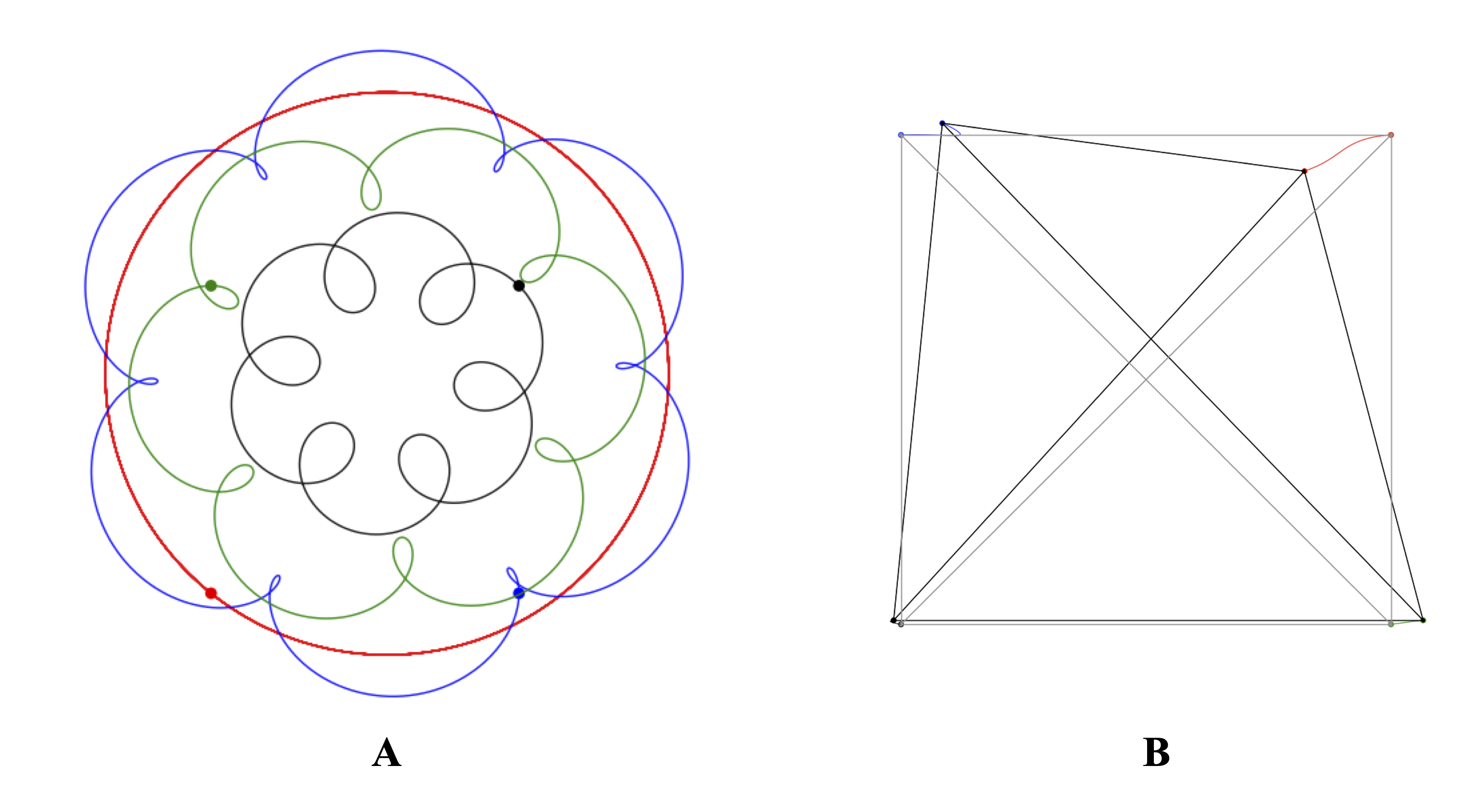
Figure 2. Flows of a square configuration with masses 1,1,3, and 5 under two different twist vector fields: (A) a fixed linear combination of three elementary twists, and (B) a gradient descent to a convex central configuration

2.2. The Hessian

In Cartesian coordinates the components of the Hessian of $f$ are

$$H_{x_{i},x_{k}}=m_{i}m_{k}\left(S_{i,k}-Ax_{i,k}^{2}T_{i,k}\right),\ \ \ \ H_{y_{i},y_{k}}=m_{i}m_{k}\left(S_{i,k}-Ay_{i,k}^{2}T_{i,k}\right),$$

$$H_{x_{i},x_{i}}=-\sum_{k\neq i}H_{x_{i},x_{k}},\ \ \ \ H_{y_{i},y_{i}}=-\sum_{k\neq i}H_{y_{i},y_{k}},$$

$$H_{x_{i},y_{k}}=-m_{i}m_{j}AT_{i,k}y_{i,k}x_{i,k},$$

$$H_{x_{i},y_{i}}=-\sum_{k\neq i}H_{x_{i},y_{k}}.$$

Using these formulae, we can compute the diagonal components of the Hessian with respect to the $v_{i,j}$:

(5) $$v_{i,j}^{T}Hv_{i,j}=-m_{i}m_{j}\left((m_{i}+m_{j})^{2}r_{i,j}^{2}S_{i,j}+\sum_{k\neq i,j}m_{k}\left[r_{i,j}^{2}(m_{j}S_{i,k}+m_{i}S_{j,k})-A\Lambda_{i,j,k}^{2}(m_{j}T_{i,k}+m_{i}T_{j,k})\right]\right).$$

The second type of entry in the Hessian in these coordinates is of the form $v_{i,j}^{T}Hv_{i,k}$ with $i$,$j$, and $k$ distinct:

(6) $$\begin{split}v_{i,j}^{T}Hv_{i,k}=&m_{i}m_{j}m_{k}\biggl{(}q_{i,j}\cdot q_{i,k}\left[m_{i}(S_{k,j}-S_{i,j}-S_{i,k})-\sum_{l\neq i}m_{l}S_{i,l}\right]+\\ &-m_{i}AT_{j,k}\Lambda_{i,j,k}^{2}-A\sum_{l\neq i,j,k}m_{l}T_{i,l}\Lambda_{i,j,l}\Lambda_{i,k,l}\biggr{)}.\end{split}$$

The last type of entry is $v_{i,j}^{T}Hv_{k,l}$ where all of $i,j,k,l$ are distinct from each other:

(7) $$\begin{split}v_{i,j}^{T}Hv_{k,l}=&m_{i}m_{j}m_{k}m_{l}\biggl{(}-A(T_{i,k}\Lambda_{i,k,l}\Lambda_{i,k,j}+T_{j,k}\Lambda_{j,k,l}\Lambda_{j,k,i}+\\ &T_{i,l}\Lambda_{i,l,k}\Lambda_{i,l,j}+T_{j,l}\Lambda_{j,l,i}\Lambda_{j,l,k})+q_{i,j}\cdot q_{k,l}(R_{i,k}+R_{j,l}-R_{j,k}-R_{i,l})\biggr{)}.\end{split}$$

Alternatively, if we just want to compute the signature of the Hessian at critical points of $f$, we can rescale the $v_{i,j}$ to

$$\tilde{v}_{i,j}=\frac{v_{i,j}}{m_{i}m_{j}r_{i,j}}.$$

Then using the notation $\mu_{i,j}=\frac{m_{i}}{m_{j}}$, $\theta_{i,j,k}$ for the angle between vectors $q_{i,j}$ and $q_{i,k}$, and $\theta_{i,j;k,l}$ for the angle between vectors $q_{i,j}$ and $q_{k,l}$, the Hessian components become

(8) $$\tilde{v}_{i,j}^{T}H\tilde{v}_{i,j}=-(2+\mu_{i,j}+\mu_{j,i})S_{i,j}+\sum_{k\neq i,j}\left[-\mu_{k,i}S_{i,k}-\mu_{k,j}S_{j,k}+A(\mu_{k,i}\sin^{2}\theta_{j,i,k}R_{i,k}+\mu_{k,j}\sin^{2}\theta_{i,j,k}R_{j,k})\right],$$

(9) $$\begin{split}\tilde{v}_{i,j}^{T}H\tilde{v}_{i,k}=&\cos\theta_{j,i,k}\left[S_{k,j}-S_{i,j}-S_{i,k}-\sum_{l\neq i}\mu_{l,i}S_{i,l}\right]\\ &-AR_{j,k}\sin\theta_{i,j,k}\sin\theta_{i,k,j}-A\sum_{l\neq i,j,k}\mu_{l,i}R_{i,l}\sin\theta_{j,i,l}\sin\theta_{k,i,l},\end{split}$$

(10) $$\begin{split}\tilde{v}_{i,j}^{T}H\tilde{v}_{k,l}=&-A(R_{i,k}\sin\theta_{i,k,l}\sin\theta_{j,i,k}+R_{j,k}\sin\theta_{j,k,l}\sin\theta_{i,j,k}+R_{i,l}\sin\theta_{i,l,k}\sin\theta_{j,i,l}\\ &+R_{j,l}\sin\theta_{j,l,k}\sin\theta_{i,j,l})+\cos\theta_{i,j;k,l}(R_{i,k}+R_{j,l}-R_{j,k}-R_{i,l}).\end{split}$$

3. Application to the 3-body problem

We will give a brief overview of the application of our equations to the 3-body case, which has been so well studied that no new results will be obtained, but it is perhaps useful to see them in this context.

For three point masses the sum in each of Laura-Andoyer equations (4) reduces to a single term:

$$\frac{\partial f}{\partial v_{i,j}}=-m_{i}m_{j}m_{k}(R_{i,k}-R_{j,k})\Lambda_{i,j,k}=0$$

in which the $i$, $j$, and $k$ are distinct. If $\Lambda_{i,j,k}$ is nonzero then $R_{i,k}=R_{j,k}$ and the points must be equidistant, so the only non-collinear central configurations are the Lagrange equilateral triangles. Any three collinear points satisfy these equations, but the $v_{i,j}$ are not independent and some additional equations must be used to recover the Euler solutions.

For the equilateral triangle with our choice of $f$, the distances $r_{i,j}=1$, and so $S_{i,j}=0$, $R_{i,j}=T_{i,j}=1$, all of the angles are $\pi/3$ so $\sin^{2}\theta_{i,j,k}=3/4$. We can compute the Hessian components:

$$\tilde{v}_{i,j}^{T}H\tilde{v}_{i,j}=\frac{3A}{4}(\mu_{k,i}+\mu_{k,j}),$$

$$\tilde{v}_{i,j}^{T}H\tilde{v}_{i,k}=-\frac{3A}{4},$$

so in coordinates $(\tilde{v}_{1,2},\tilde{v}_{1,3},\tilde{v}_{2,3})$ the Hessian matrix is

$$\frac{3A}{4}\left(\begin{array}[]{ccc}\mu_{3,1}+\mu_{3,2}&-1&-1\\ -1&\mu_{2,1}+\mu_{2,3}&-1\\ -1&-1&\mu_{1,2}+\mu_{1,3}\end{array}\right).$$

This matrix has one zero eigenvalue corresponding to the rotational symmetry of the space, and two positive eigenvalues. To prove positivity of the nonzero eigenvalues we first note that the matrix is symmetric, so its eigenvalues are real. Its characteristic polynomial factors as $\lambda(a_{0}+a_{1}\lambda+a_{2}\lambda)$, in which the coefficients $a_{i}$ are functions of the mass ratios $\mu_{j,k}$. The reality of the eigenvalues means that the discriminant $a_{1}^{2}-4a_{0}a_{2}\geq 0$, and it is straightforward to compute that the functions $a_{0}$ and $a_{2}$ have the same sign, so $a_{1}>\sqrt{a_{1}^{2}-4a_{0}a_{2}}$. It is also straightforward to compute that

$$a_{1}=-(\mu_{1,2}+\mu_{1,3}+\mu_{2,3}+\mu_{2,1}+\mu_{3,1}+\mu_{3,2})<0$$

so the eigenvalues $-a_{1}/2\pm\sqrt{a_{1}^{2}-4a_{0}a_{2}}/2$ are positive, and the Lagrange configurations are minima of $f$.

4. Application to the 4-body problem

We will illustrate the utility of our new equations for the Hessian by computing the Morse index of the four-body central configurations which are concave isosceles triangles (sometimes called concave kites). This includes the case of equilateral triangles with one arbitrary nonnegative central mass and three equal outer masses. This is an interesting special case since it has long been known to possess a degenerate Hessian for particular ratios of the central to outer masses [33, 27, 28, 39].

There are several bifurcations in the index of the Hessian, which correspond to some of the changes in number of concave central configurations seen for example in [40].

Our coordinates for the four points will be $q_{1}=(-x_{2},0)$, $q_{2}=(x_{2},0)$, $q_{3}=(0,y_{3})$, and $q_{4}=(0,y_{4})$. We will assume that $x_{2}$ is positive and $y_{3}>y_{4}$. With elementary geometry we can compute:

$$\Lambda_{1,2,3}=2x_{2}y_{3},\ \ \ \Lambda_{1,2,4}=2x_{2}y_{4},\ \ \ \Lambda_{1,3,4}=-\Lambda_{2,3,4}=x_{2}(y_{3}-y_{4}),$$

$$\sin\theta_{1,2,3}=\frac{y_{3}}{r_{1,3}},\ \ \ \sin\theta_{1,2,4}=\frac{y_{4}}{r_{1,4}},\ \ \ \sin\theta_{1,3,2}=\frac{r_{1,2}y_{3}}{r_{1,3}^{2}},\ \ \ \sin\theta_{1,4,2}=\frac{r_{1,2}y_{4}}{r_{1,4}^{2}},$$

$$\sin\theta_{1,3,4}=\frac{r_{1,2}}{2r_{1,3}},\ \ \ \ \sin\theta_{3,1,4}=\frac{r_{3,4}r_{1,2}}{2r_{1,3}r_{1,4}},\ \ \ \ \sin\theta_{1,4,3}=\frac{r_{1,2}}{2r_{1,4}},$$

$$\cos\theta_{1,3,2}=1-\frac{r_{1,2}^{2}}{2r_{1,3}^{2}},\ \ \ \cos\theta_{1,3;2,4}=\frac{y_{3}y_{4}-x_{2}^{2}}{r_{1,3}r_{1,4}}.$$

One of the critical point equations (4) implies that $m_{1}=m_{2}$, and the others which are nontrivial simplify to

$$\frac{1}{m_{1}m_{3}}\frac{\partial f}{\partial v_{1,3}}=-2m_{1}(R_{1,2}-R_{1,3})x_{2}y_{3}+m_{4}(R_{1,4}-R_{3,4})x_{2}r_{3,4}=0,$$

$$\frac{1}{m_{1}m_{4}}\frac{\partial f}{\partial v_{1,4}}=-2m_{1}(R_{1,2}-R_{1,4})x_{2}y_{4}-m_{3}(R_{1,3}-R_{3,4})x_{2}r_{3,4}=0,$$

so the mass ratios are

(11) $$\mu_{3,1}=\frac{m_{3}}{m_{1}}=\frac{2y_{4}}{r_{3,4}}\frac{(R_{1,4}-R_{1,2})}{(R_{3,4}-R_{1,3})},$$

(12) $$\mu_{4,1}=\frac{m_{4}}{m_{1}}=\frac{2y_{3}}{r_{3,4}}\frac{(R_{1,2}-R_{1,3})}{(R_{1,4}-R_{3,4})}.$$

Besides the equilateral case, there are two classes of concave kites with non-negative masses. If $\frac{y_{3}}{x_{2}}>\sqrt{3}$, then $r_{1,3}=r_{2,3}>r_{1,2}$ and $\frac{y_{3}}{2}-\frac{x_{2}^{2}}{2y_{3}}<y_{4}<\frac{x_{2}\sqrt{3}}{2}$. Alternatively if $y_{3}<\frac{\sqrt{3}}{2}$ then for non-negative masses we must have $0<y_{4}<\frac{y_{3}}{2}-\frac{x_{2}^{2}}{2y_{3}}$. When $y_{4}=\frac{y_{3}}{2}-\frac{x_{2}^{2}}{2y_{3}}$, the fourth point is at the circumcenter of the outer triangle, and $r_{1,4}=r_{2,4}=r_{3,4}$.

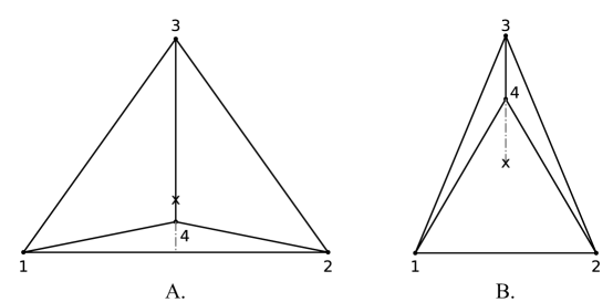
Figure 3. Two examples of concave kites. A. An example ‘wide’ kite with $r_{1,3}=r_{2,3}<r_{1,2}$; the fourth point must be below the circumcenter (marked with an ‘x’) for positive mass configurations. B. An example ‘tall’ kite with $r_{1,3}=r_{2,3}>r_{1,2}$; the fourth point must be above the circumcenter.

The Dziobek equations [12, 30]:

$$S_{1,2}S_{3,4}=S_{1,3}S_{2,4}=S_{1,4}S_{2,3}$$

in the case of the isosceles kites specialize to just one equation,

(13) $$S_{1,2}S_{3,4}=S_{1,3}S_{1,4}.$$

This Dziobek equation can be used to find $x_{2}=r_{1,2}/2$ given the shape variables $z_{3}=\frac{y_{3}}{x_{2}}$ and $z_{4}=\frac{y_{4}}{x_{2}}$:

(14) $$x_{2}=\frac{1}{2}\left(\frac{(z_{3}-z_{4})^{-A}-(1+z_{3}^{2})^{-A}(1+z_{4}^{2})^{-A}}{1+(z_{3}-z_{4})^{-A}-(1+z_{3}^{2})^{-A}-(1+z_{4}^{2})^{-A}}\right)^{1/A}.$$

We can block-diagonalize the Hessian for these kites by using the basis

$$\beta=[\tilde{v}_{a,3}=\frac{1}{\sqrt{2}}(\tilde{v}_{1,3}+v_{2,3}),\ \ \ \tilde{v}_{a,4}=\frac{1}{\sqrt{2}}(v_{1,4}+v_{2,4}),\ \ \ \ \tilde{v}_{3,4},$$

$$\tilde{v}_{s,3}=\frac{1}{\sqrt{2}}(\tilde{v}_{1,3}-\tilde{v}_{2,3}),\ \ \ \tilde{v}_{s,4}=\frac{1}{\sqrt{2}}(v_{1,4}-v_{2,4})],$$

which results in blocks of dimensions $3\times 3$ and $2\times 2$, which we will denote by $H_{a}$ and $H_{s}$ respectively.

The $H_{a}$ block always contains the eigenvector of eigenvalue 0 which is tangent to the uniform rotation about the center of mass. While it is possible to symbolically calculate this eigenvector in these coordinates, it is quite complicated, and it does not seem productive to calculate the resulting residual $2\times 2$ submatrix explicitly.

The $2\times 2$ block $H_{s}$ is easier to analyze, and it contains an interesting bifurcation. We will focus on the configurations that are close to the coorbital case, in which the fourth point is close to the circumcenter of the outer three points. The first component of $H_{s}$ is

$$(H_{s})_{1,1}=\frac{1}{2}\left(\tilde{v}_{1,3}^{T}H\tilde{v}_{1,3}+\tilde{v}_{2,3}^{T}H\tilde{v}_{2,3}-2\tilde{v}_{1,3}^{T}H\tilde{v}_{2,3}\right)$$

$$=\tilde{v}_{1,3}^{T}H\tilde{v}_{1,3}-\tilde{v}_{1,3}^{T}H\tilde{v}_{2,3}$$

$$=-(2+\mu_{1,3}+\mu_{3,1})S_{1,3}+\sum_{k\neq 1,3}\left[-\mu_{k,1}S_{1,k}-\mu_{k,3}S_{3,k}+A(\mu_{k,1}\sin^{2}\theta_{3,1,k}R_{1,k}+\mu_{k,3}\sin^{2}\theta_{1,3,k}R_{3,k})\right]$$

$$-\left(\cos\theta_{1,3,2}\left[S_{1,2}-S_{1,3}-S_{2,3}-\sum_{l\neq 3}\mu_{l,3}S_{3,l}\right]-AR_{1,2}\sin\theta_{3,1,2}\sin\theta_{3,2,1}-A\mu_{4,3}R_{3,4}\sin\theta_{1,3,4}\sin\theta_{2,3,4}\right)$$

$$=-(2+2\mu_{1,3}+\mu_{3,1})S_{1,3}-S_{1,2}-\mu_{4,1}S_{1,4}-\mu_{4,3}S_{3,4}-\left(1-\frac{r_{1,2}^{2}}{2r_{1,3}^{2}}\right)\left(S_{1,2}-2S_{1,3}-2\mu_{1,3}S_{1,3}-\mu_{4,3}S_{3,4}\right)$$

$$+A\left(\frac{2y_{3}^{2}}{r_{1,3}^{2}}R_{1,2}+\mu_{2,3}\frac{r_{1,2}^{2}y_{3}^{2}}{r_{1,3}^{2}}R_{1,3}+\mu_{4,1}\frac{r_{1,2}^{2}r_{3,4}^{2}}{4r_{1,3}^{2}r_{1,4}^{2}}R_{1,4}+2\mu_{4,3}\frac{r_{1,2}^{2}}{4r_{1,3}^{2}}R_{3,4}\right).$$

Similarly

$$(H_{s})_{2,2}=\tilde{v}_{1,4}^{T}H\tilde{v}_{1,4}-\tilde{v}_{1,4}^{T}H\tilde{v}_{2,4}$$

$$=-(2+\mu_{1,4}+\mu_{4,1})S_{1,4}+\sum_{k\neq 1,4}\left[-\mu_{k,1}S_{1,k}-\mu_{k,4}S_{4,k}+A(\mu_{k,1}\sin^{2}\theta_{4,1,k}R_{1,k}+\mu_{k,4}\sin^{2}\theta_{1,4,k}R_{4,k})\right]$$

$$-\left(\cos\theta_{1,4,2}\left[S_{1,2}-S_{4,1}-S_{4,2}-\sum_{l\neq 4}\mu_{l,4}S_{4,l}\right]-AR_{1,2}\sin\theta_{4,1,2}\sin\theta_{4,2,1}-A\mu_{3,4}R_{3,4}\sin\theta_{1,4,3}\sin\theta_{2,4,3}\right)$$

$$=-(2+2\mu_{1,4}+\mu_{4,1})S_{1,4}-S_{1,2}-\mu_{3,1}S_{1,3}-\mu_{3,4}S_{3,4}-\left(1-\frac{r_{1,2}^{2}}{2r_{1,4}^{2}}\right)\left(S_{1,2}-2S_{1,4}-2\mu_{1,4}S_{1,4}-\mu_{3,4}S_{3,4}\right)$$

$$+A\left(\frac{2y_{4}^{2}}{r_{1,4}^{2}}R_{1,2}+\mu_{2,4}\frac{r_{1,2}^{2}y_{4}^{2}}{r_{1,4}^{2}}R_{1,4}+\mu_{3,1}\frac{r_{1,2}^{2}r_{3,4}^{2}}{4r_{1,3}^{2}r_{1,4}^{2}}R_{1,3}+2\mu_{3,4}\frac{r_{1,2}^{2}}{4r_{1,4}^{2}}R_{3,4}\right),$$

and

$$(H_{s})_{1,2}=(H_{s})_{2,1}=\tilde{v}_{1,3}^{T}H\tilde{v}_{1,4}+\tilde{v}_{1,3}^{T}H\tilde{v}_{2,4},$$

in which

$$\tilde{v}_{1,3}^{T}H\tilde{v}_{2,4} =\cos{\theta_{1,3;2,4}}(R_{1,2}+R_{3,4}-R_{1,3}-R_{1,4})-A(R_{1,2}\sin{\theta_{1,2,4}}\sin{\theta_{3,1,2}}$$

$$+ R_{1,3}\sin{\theta_{3,1,4}}\sin{\theta_{1,3,2}}+R_{1,4}\sin{\theta_{1,4,2}}\sin{\theta_{3,1,4}}+R_{3,4}\sin{\theta_{3,4,2}}\sin{\theta_{1,3,4}})$$

$$=\frac{1}{r_{1,3}r_{1,4}}\left[(y_{3}y_{4}-x_{2}^{2})(R_{1,2}+R_{3,4}-R_{1,3}-R_{1,4})\right.$$

$$\left.-A\left(R_{1,2}y_{3}y_{4}+R_{1,3}\frac{r_{1,2}^{2}r_{3,4}y_{3}}{2r_{1,3}^{2}}+R_{1,4}\frac{r_{1,2}^{2}r_{3,4}y_{4}}{2r_{1,4}^{2}}+R_{3,4}\frac{r_{1,2}^{2}}{4}\right)\right],$$

and

$$\tilde{v}_{1,3}^{T}H\tilde{v}_{1,4} =\cos\theta_{3,1,4}\left(S_{3,4}-S_{1,3}-S_{1,4}-\mu_{2,1}S_{1,2}-\mu_{3,1}S_{1,3}-\mu_{4,1}S_{1,4}\right)$$

$$-AR_{3,4}\sin\theta_{1,3,4}\sin\theta_{1,4,3}-A\mu_{2,1}R_{1,2}\sin\theta_{3,1,2}\sin\theta_{1,2,4}$$

$$=\frac{1}{4r_{1,3}r_{1,4}}\left\{(r_{1,2}^{2}+4y_{3}y_{4})\Bigl{[}S_{3,4}-(1+\mu_{3,1})S_{1,3}-(1+\mu_{4,1})S_{1,4}-S_{1,2}\Bigr{]}\right.$$

$$\left.-A(R_{3,4}r_{1,2}^{2}-4R_{1,2}y_{3}y_{4})\right\}.$$

The eigenvalues of these Hessians contain several bifurcations depending the shape of the isosceles configuration and the exponent parameter $A$, which are difficult to analytically characterize in general. For the Newtonian case we investigated the Hessian eigenvalues more thoroughly numerically. Most of these numerical conclusions can be refined to rigorous results using interval arithmetic, since there are only two shape parameters, and our block diagonalization of the Hessian greatly reduces the computations.

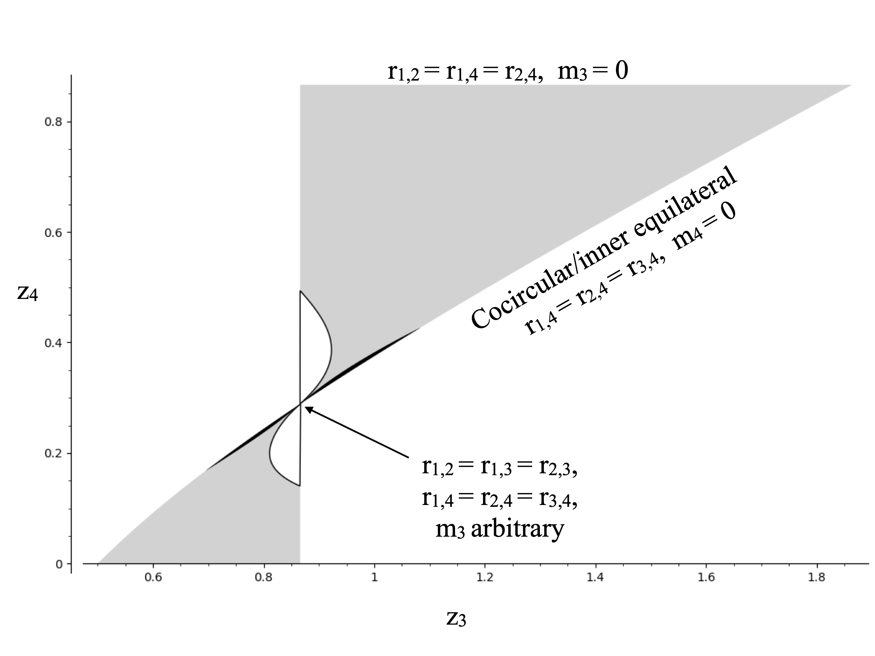
Figure 4. Isosceles kite central configurations for the Newtonian potental with nonnegative masses parameterized by $z_{3}$ and $z_{4}$. Configurations with a positive-definite Hessian are shaded in white; Hessians of index 3 are shaded in grey, and Hessians of index 2 are black.

In Figure 4 we illustrate the concave isosceles configurations parameterized by $z_{3}$ and $z_{4}$.

When $z_{4}=y_{c}$ the fourth point is at the circumcenter of the outer triangle formed by the first three points, so $r_{1,3}=r_{2,3}=r_{3,4}$. To have a central configuration with positive masses we must have $z_{4}>y_{c}$. As $z_{4}$ approaches $y_{c}$ we obtain in the limit the $1+3$ coorbital central configurations, which have been extensively characterized already [36, 10, 11].

From equations (11) and (12) we see that for a fixed outer triangle shape as $z_{4}$ approaches $y_{c}$ the ratio of $m_{4}$ to the outer masses becomes infinite. Some terms in the Hessian that contain $\mu_{4,1}$ or $\mu_{4,3}$ will then dominate the others. There is some subtlety in products such as $\mu_{4,1}S_{1,4}$ however, since the inner distances become close to $1$ in this limit, $S_{1,4}$ and $S_{3,4}$ approach 0. We can handle these quantities by using the critical point relation $U=MI$ described earlier, and the Dziobek equation (13). From this relation we can see that $R_{1,4}$ and $R_{3,4}$ must approach $1$ as $z_{4}$ approaches $y_{c}$ if the outer shape is fixed.

If we divide the relation $U-MI=0$ by $m_{1}^{2}$, for the isosceles central configurations we have

$$r_{1,2}^{2}S_{1,2}+2\mu_{3,1}r_{1,3}^{2}S_{1,3}+2\mu_{4,1}r_{1,4}^{2}S_{1,4}+\mu_{4,1}\mu_{3,1}r_{3,4}^{2}S_{3,4}=0.$$

Eliminating $S_{3,4}$ with the Dziobek equation we can express $\mu_{4,1}S_{1,4}$ in terms of quantities with more obvious limits:

$$\mu_{4,1}S_{1,4}=-\frac{r_{1,2}^{2}S_{1,2}+2\mu_{3,1}r_{1,3}^{2}S_{1,3}}{2r_{1,4}^{2}+\mu_{3,1}r_{3,4}^{2}S_{1,3}/S_{1,2}}.$$

The $H_{s}$ submatrix of the Hessian is responsible for the upper ($z_{3}>\sqrt{3}/2$) black to grey bifurcation in Figure 4, where the Hessian changes from index 2 to index 1, and the lower white to grey bifurcation ($z_{3}<\sqrt{3}/2$) in which the Hessian changes from index 0 to index 1. In the index 2 configurations, one negative eigenvalue comes from $H_{a}$ and one from $H_{s}$, with the boundary determined by the change of a positive to a negative eigenvalue in $H_{s}$ or $H_{a}$ for the upper or lower change, respectively. Similarly, the white shaded region corresponds to configurations with index 0, the boundary of which is defined by a zero eigenvalue of $H_{a}$ for the upper region and $H_{s}$ for the lower region. These switches between the responsible submatrix were surprising to us. = We can verify the picture in Figure 4 with interval arithmetic to a resolution which is at least an order of magnitude better than in the figure. It is difficult to completely prove the indicated structure of the bifurcations, especially near the boundaries where some of the masses approach zero, and the most symmetric point where $r_{1,2}=r_{1,3}=r_{2,3}$ and $r_{1,4}=r_{2,4}=r_{3,4}$. Some changes in variables similar to equation (14) could probably be used near the boundaries to fix these issues, but there the problem reduces to the restricted problem, which has been previously well characterized [25, 34, 35, 14, 5, 24, 6]. Near the symmetric point, where the mass $m_{4}$ is arbitary, a perturbative analysis has been done for some aspects of the central configurations [27].

It would be interesting to see if these bifurcation curves could be computed exactly, for example with Gröbner bases, which seems quite possible; we did not attempt that.

5. Conclusion and future directions

To the best of our knowledge the framework of the twist vectors introduced here has not been described before, although because of the relative simplicity of the idea it is very possible that it occurs elsewhere in the classical mechanics literature.

Although our equations are not very simple, in a standard Cartesian basis the Hessian of the function $f$ is much more complicated and harder to interpret in terms of geometric quantities. We hope the approach presented here can be used to improve results on the finiteness, enumeration, and stability analysis of relative equilibria and central configurations in the $N$-body family of problems.

References

• [1] A. Albouy, H. E. Cabral, and A. A. Santos, Some problems on the classical n-body problem, Cel. Mech. Dyn. Astron. 113 (2012), no. 4, 369–375.
• [2] A. Albouy and A. Chenciner, Le problème des n corps et les distances mutuelles, Invent. math. 131 (1997), no. 1, 151–184.
• [3] H. Andoyer, Sur l’équilibre relatif de n corps, Bull. Astron. V. 23 (1906), 50–59.
• [4] H. Aref, N. Rott, and H. Thomann, Gröbli’s solution of the three-vortex problem, Annual Review of Fluid Mechanics 24 (1992), no. 1, 1–21.
• [5] R. F. Arenstorff, Central configurations of four bodies with one inferior mass, Cel. Mech. 28 (1982), 9–15.
• [6] J. F. Barros and E. S. G. Leandro, Bifurcations and enumeration of classes of relative equilibria in the planar restricted four-body problem, SIAM J. Math. Anal. 46 (2014), no. 2, 1185–1203.
• [7] V. L. Barutello, R. D. Jadanza, and A. Portaluri, Linear instability of relative equilibria for n-body problems in the plane, J. of Diff. Eq. 257 (2014), no. 6, 1773–1813.
• [8] R. Bott, Morse theory indomitable, Publications Mathématiques de l’Institut des Hautes Études Scientifiques 68 (1988), no. 1, 99–114.
• [9] J. Chazy, Sur certaines trajectoires du problème des n corp, Bull. Astronom. 35 (1918), 321–389.
• [10] M. Corbera, J. M. Cors, J. Llibre, and R. Moeckel, Bifurcation of relative equilibria of the (1+ 3)-body problem, SIAM Journal on Mathematical Analysis 47 (2015), no. 2, 1377–1404.
• [11] Y. Deng, M. Hampton, and Z. Wang, Symmetry and asymmetry in the 1+N coorbital problem, SIAM Journal on Applied Dynamical Systems 21 (2022), no. 3, 2080–2095.
• [12] O. Dziobek, Über einen merkwürdigen Fall des Vielkörperproblem, Astron. Nachr. 152 (1900), 33–46.
• [13] L. Euler, De motu rectilineo trium corporum se mutuo attrahentium, Novi Comm. Acad. Sci. Imp. Petrop 11 (1767), 144–151.
• [14] J. R. Gannaway, Determination of all central configurations in the planar four-body problem with one inferior mass, Ph.D. thesis, Vanderbilt University, TN, 1981.
• [15] M. Gascheau, Examen d’une classe d’équations différentielles et application à un cas particulier du probl’éme des trois corps, Compt. Rend. 16 (1843), 393–394.
• [16] Y. Hagihara, Celestial mechanics vol. 1, Celestial Mechanics, MIT Press, 1970.
• [17] M. Hampton, Planar n-body central configurations with a homogeneous potential, Cel. Mech. Dyn. Astron. 131 (2019), no. 20.
• [18] M. Hampton and R. Moeckel, Finiteness of relative equilibria of the four-body problem, Invent. math. 163 (2005), no. 2, 289–312.
• [19] H. Helmholtz, Über Integrale der hydrodynamischen Gleichungen, welche den Wirbelbewegungen entsprechen, Crelle’s Journal für Mathematik 55 (1858), 25–55, English translation by P. G. Tait, P.G., On the integrals of the hydrodynamical equations which express vortex-motion, Philosophical Magazine, (1867) 485-51.
• [20] X. Hu and S. Sun, Stability of relative equilibria and Morse index of central configurations, C. R. Acad. Sci. Paris 347 (2009), 1309–1312.
• [21] G. Kirchhoff, Vorlesungen über mathematische Physik, B.G. Teubner, 1883.
• [22] J. L. Lagrange, Essai sur le problème des trois corps, Œuvres, vol. 6, Gauthier-Villars, Paris, 1772.
• [23] E. Laura, Sulle equazioni differenziali canoniche del moto di un sistema di vortici elementari rettilinei e paralleli in un fluido incomprensibile indefinito, Atti della Reale Accad. Torino 40 (1905), 296–312.
• [24] E. S. G. Leandro, On the central configurations of the planar restricted four-body problem, J. Diff. Eq. 226 (2006), no. 1, 323–351.
• [25] M. Lindlow, Ein Spezialfall des Vierkörperproblems, Astron. Nachr. 216 (1922), 233–248.
• [26] G Meyer, Solutions voisines des solutions de Lagrange dans le probleme des n corps, Annales de l’Observatoire de Bordeaux, vol. 17, pp. 77-252 17 (1933), 77–252.
• [27] K. R. Meyer and D. S. Schmidt, Bifurcations of relative equilibria in the 4-and 5-body problem, Ergod. Th. & Dynam. Sys 8 (1988), 215–225.
• [28] by same author, Bifurcations of relative equilibria in the N-body and Kirchhoff problems, SIAM J. Math. Anal. 19 (1988), no. 6, 1295–1313.
• [29] J. Milnor, Morse theory, vol. 51, Princeton University press, 2016.
• [30] R. Moeckel, Generic finiteness for Dziobek configurations, Trans. Amer. Math. Soc. 353 (2001), no. 11, 4673–4686.
• [31] by same author, Central Configurations, Central Configurations, Periodic Orbits, and Hamiltonian Systems, Springer, 2015.
• [32] J. Montaldi, Existence of symmetric central configurations, Cel. Mech. Dyn. Astr. 122 (2015), 405–418.
• [33] J. I. Palmore, Relative equilibria of the $n$-body problem, Ph.D. thesis, University of California, Berkeley, CA, 1973.
• [34] P. Pedersen, Librationspunkte im Restringierten Vierkoerperproblem, Publikationer og mindre Meddeler fra Kobenhavns Observatorium 137 (1944), 1–80.
• [35] by same author, Stabilitätsuntersuchungen im Restringierten Vierkörperproblem, Publikationer og mindre Meddeler fra Kobenhavns Observatorium 159 (1952), 1–38.
• [36] S. Renner and B. Sicardy, Stationary configurations for co-orbital satellites with small arbitrary masses, Cel. Mech. Dyn. Astron. 88 (2004), no. 4, 397–414.
• [37] G. E. Roberts, Linear stability of the elliptic Lagrangian triangle solutions in the three-body problem, J. of Diff. Eq. 182 (2002), 191–218.
• [38] E. J. Routh, On Laplace’s three particles with a supplement on the stability of their motion, Proc. London Math. Soc. 6 (1875), 86–97.
• [39] A. A. Santos, M. Marchesin, E. Pérez-Chavela, and C. Vidal, Continuation and bifurcations of concave central configurations in the four and five body-problems for homogeneous force laws, J. Math. Anal. Appl. 446 (2017), 1743–1768.
• [40] C. Simo, Relative equilibrium solutions in the four body problem, Cel. Mech. Dyn. Astron. 18 (1978), no. 2, 165–184.
• [41] S. Smale, Mathematical problems for the next century, Mathematical Intelligencer 20 (1998), 7–15.
• [42] A. Wintner, The analytical foundations of celestial mechanics, Princeton University Press, Princeton, NJ, 1941.