Piecewise Constant Tuning Gain Based Singularity-Free MRAC with Application to Aircraft Control Systems

Abstract

This paper introduces an innovative singularity-free output feedback model reference adaptive control (MRAC) method applicable to a wide range of continuous-time linear time-invariant (LTI) systems with general relative degrees. Unlike existing solutions such as Nussbaum and multiple-model-based methods, which manage unknown high-frequency gains through persistent switching and repeated parameter estimation, the proposed method circumvents these issues without prior knowledge of the high-frequency gain or additional design conditions. The key innovation of this method lies in transforming the estimation error equation into a linear regression form via a modified MRAC law with a piecewise constant tuning gain developed in this work. This represents a significant departure from existing MRAC systems, where the estimation error equation is typically in a bilinear regression form. The linear regression form facilitates the direct estimation of all unknown parameters, thereby simplifying the adaptive control process. The proposed method preserves closed-loop stability and ensures asymptotic output tracking, overcoming some of the limitations associated with existing methods like Nussbaum and multiple-model based methods. The practical efficacy of the developed MRAC method is demonstrated through detailed simulation results within an aircraft control system scenario.

I Introduction

With the increasing demand for robustness and control accuracy of control systems in manufacturing, aerospace and other fields, adaptive control has attracted extensive attention from researchers because of its remarkable adaptability to system uncertainties. So far, adaptive control has made significant progress, with many valuable research results being reported ([26, 12, 10, 38, 1, 13, 3, 5, 7, 31, 18]).

In recent decades, the field of control systems has seen rapid advancements in model reference adaptive control (MRAC) ([10, 2, 28, 21, 40, 37]). In the traditional MRAC framework, a key feature is the coupling between the unknown high-frequency gain and the unknown estimation error associated with the system parameters, from which the estimation error equation caused by this interaction takes on a form of bilinear regression. To address this issue, the majority of output feedback MRAC methods, such as the renowned augmented error-based method ([10, 28]), choose a strategy that incorporate the high-frequency gain information. This information is utilized to design parameter update laws and prevent the singularity of MRAC laws. However, these design constraints on the high-frequency gain hinder the further development of MRAC and its application in systems with unknown control directions. Relaxing these design constraints on the high-frequency gain has consistently been a prominent research topic in the control community.

For an extended period, researchers have been dedicated to addressing this problem, leading to the development of numerous enhanced adaptive control methods ([15, 24, 30, 6, 11, 33, 14]). In [22], a Nussbaum function was first introduced into the control signal, where the prior knowledge about the high-frequency gain is no longer required. Since then, the adaptive control approaches on the basis of Nussbaum function have been widely reported ([36, 39, 16, 9]). However, this method may exhibit oscillation and persistent switching issues, as shown in [27, 35]. Another well-known method to addressing the issue of high-frequency gain sign is the multiple-model-based control technique, first developed in [19]. This approach has attracted significant attention from researchers ([17, 20, 8]). The multiple-model-based control method requires repeated estimation of plant parameters and may also exhibit the persistent switching issue, as mentioned in [17]. Additionally, the design constraints on the sign of the high-frequency gain can also be removed by introducing alternative design conditions, such as assuming that the bounds of the high-frequency gain are known ([15]) or that the signal is interval exciting ([32]).

Reviewing the literature reveals that researchers have made significant long-term efforts to address the high-frequency gain sign problem, achieving numerous remarkable results. However, some open issues remain unresolved. Recently, for continuous-time linear time-invariant (LTI) systems, a modified MRAC method was developed in [23] by employing a standard Lyapunov stability analysis. This method relaxes the design constraints on the high-frequency gain by injecting the estimation of the tracking error derivative into the control signal, while mitigating the persistent switching issue commonly involved in the well-known Nussbaum-based and multiple-model-based methods. Motivated by [23], [34] proposed a singularity-free output feedback MRAC method for a general class of discrete-time LTI systems, which eliminates the need for high-frequency gain sign and bound information commonly used in discrete-time MRAC systems. The development of an output feedback MRAC scheme that operates independently of prior knowledge concerning high-frequency gain across a general class of continuous-time LTI systems, particularly those with general relative degrees, presents considerable challenges. These challenges stem primarily from the need to circumvent issues associated with persistent switching and the continual re-estimation of parameters. It should be emphasized that the stability analysis presented in [23] relies on conventional Lyapunov techniques and is tailored specifically to MRAC systems with a relative degree of one. Moreover, the control methodology delineated in [34], although effective for discrete-time systems, is ill-suited for the regulation of continuous-time systems that exhibit general relative degrees. This incompatibility arises due to inherent differences in the stability properties between continuous and discrete-time systems. Consequently, there is a pronounced need for a unified, singularity-free output feedback MRAC framework that is adaptable to continuous-time LTI systems without requiring any foreknowledge of the high-frequency gain. This gap underscores a significant and yet unexplored area within the field of adaptive control.

In this paper, we address the challenge of adaptive control gain singularity in a general class of continuous-time LTI systems with general relative degrees. The fundamental strategy employed involves the decoupling of high-frequency gain from the parameters of the derived control law. This critical decoupling enables the transformation of the estimation error equation into a linear regression model, distinctively diverging from the conventional bilinear model used in traditional MRAC frameworks. Such an approach allows for the design of the parameter update law directly, eliminating the dependency on prior knowledge of the high-frequency gain. The significant contributions of this research are outlined as follows:

1. We develop a novel output feedback MRAC framework applicable to a comprehensive range of continuous-time LTI systems with general relative degrees. The proposed MRAC law is meticulously designed to ensure the boundedness of all signals within the closed-loop system, as well as to achieve asymptotic output tracking of the target plant, all accomplished without any reliance on prior knowledge regarding the high-frequency gain.

2. The estimation error equation is transformed into a linear regression form, facilitated by a modified MRAC framework developed in this paper. This represents a significant departure from traditional MRAC systems, where the estimation error equation takes on a bilinear regression form. The adoption of the linear regression form enables direct estimation of all unknown parameters, thereby simplifying the adaptive control process.

3. A new adaptive control law with piecewise constant tuning gain is proposed to address the persistent switching and repeated parameter estimation issues, ensuring singularity-free operation. Unlike the primary approaches, Nussbaum and multiple-model based techniques, which handle unknown high-frequency gains through persistent switching and repeated parameter estimation, the proposed solution overcomes these issues despite lacking high-frequency gain information or additional design conditions.

The rest of this paper is structured as follows. In Section 2, we describe the controlled plant and clarify the technical issues to be addressed. In Section 3, we give the design details of the proposed adaptive control scheme. In Section 4, we show the simulation results. In Section 5, we conclude the work of this paper.

Notation: Let a finite-dimensional vector $X(t)=[X_{1}(t),...,X_{n}(t)]^{T}\in\mathbb{R}^{n}$. The signal space $L^{2}$ is defined as the set $\{X(t):(\int_{0}^{\infty}(X_{1}^{2}(t)+\cdots+X_{n}^{2}(t))dt)^{1/2}<\infty\}$, encapsulating vectors whose squared components integrated over time yield a finite result. Conversely, the signal space $L^{\infty}$ comprises vectors $X(t)$ for which $\sup_{t\geq 0}\max_{1\leq i\leq n}|X_{i}(t)|<\infty$, indicating that each component’s absolute value remains bounded over time. For any constant $A$, the function $\operatorname{sign}(A)$ represents the sign of $A$. In the context of matrix algebra, for a matrix $B\in\mathbb{R}^{n\times n}$, the notation $B\succ 0$ signifies that $B$ is positive definite, indicating all eigenvalues are strictly positive. The operator $s$ is employed to denote two types of operations: $sX=\mathcal{L}(X(t))$ representing the Laplace transform of $X(t)$, or $sX=\dot{X}(t)$ representing the derivative of $X(t)$. The function $y(t)=G(s)[u](t)$ describes the output $y(t)$ of a continuous-time linear time-invariant system characterized by the transfer function $G(s)$, with $u(t)$ as its input. This notation is integral to adaptive control literature (referenced in [28, 5, 10]) as it amalgamates operations in both the time domain and the complex frequency domain, thus obviating the necessity for complex convolutional expressions in the analysis of control systems.

II Problem statement

This section provides a description of the controlled plant and outlines the technical issues that need to be addressed.

II-A System model

Consider a class of LTI systems, which are characterized by their input-output relationship in the following form:

$$P(s)[y](t)=k_{p}Z(s)[u](t),$$ (1)

where this relationship holds for all $t\geq 0$. Here, $y(t)\in\mathbb{R}$ and $u(t)\in\mathbb{R}$ represent the output and input of the system, respectively. The system dynamics are governed by the polynomials $P(s)$ and $Z(s)$, defined as:

$$P(s) = s^{n}+p_{n-1}s^{n-1}+\cdots+p_{1}s+p_{0},$$

$$Z(s) = s^{m}+z_{m-1}s^{m-1}+\cdots+z_{1}s+z_{0}.$$

The coefficients $p_{i}$ and $z_{j},0\leq i\leq n-1,0\leq j\leq m-1$, are unknown. Additionally, $k_{p}$, representing an unknown non-zero constant high-frequency gain, plays a crucial role in the system’s response. The relative degree of the system, denoted as $n^{*}=n-m$, can be arbitrary, such that $1\leq n^{*}\leq n$, reflecting the differential order between the system’s output and input dynamics.

The reference model in our study is defined by the following relationship:

$$y^{*}(t)=W^{*}(s)[r](t),$$ (2)

where $y^{*}(t)$ denotes the reference output, characterized by bounded derivatives up to the $n^{*}$ order. The function $W^{*}(s)$ represents a stable transfer function, and $r(t)$ is the reference input, which is also bounded along with its first derivative. As outlined in prior studies [10, 28], $W^{*}(s)$ is typically selected as $\frac{1}{R_{m}(s)}$ where $R_{m}(s)$ is a monic Hurwitz polynomial with a degree equal to $n^{*}$.

II-B Control objective and design conditions

This paper is dedicated to the development of a singularity-free output feedback adaptive control law for the system described in (1), where all parameters, including $p_{i}$, $z_{j}$, and $k_{p}$, are assumed to be unknown. Our objective is to ensure the closed-loop stability of this system and achieve asymptotic tracking convergence, specifically that $\lim_{t\rightarrow\infty}(y(t)-y^{*}(t))=0$.

To advance our design and analysis, we establish the following assumptions:

(A1) The polynomial $Z(s)$ is Hurwitz, ensuring that it has all poles in the left half of the complex plane.

(A2) The degree $n$ of the polynomial $P(s)$ is known.

(A3) The system relative degree $n^{*}$ is known.

The closed-loop MRAC system involves zero-pole cancellation, and Assumption (A1) ensures that this cancellation is stable. Assumption (A2) determines the dimension of the parameters to be estimated, while Assumption (A3) pertains to the selection of $W^{*}(s)$. These assumptions represent the design conditions required for the traditional MRAC framework [10, 21, 28]. Assumption (A2) can be relaxed if an upper bound on $n$ is known, and similarly, Assumption (A3) can be moderated if an upper limit on $n^{*}$ is established. These adaptations, as discussed in [10, 21, 28], permit a more versatile control design framework that accommodates uncertainties in the system’s dynamic orders, thereby facilitating effective adaptive control performance under less rigid conditions. Relaxing Assumptions (A2) and (A3) leads to increased complexity and additional computational demands. Due to the scope of this paper, we do not explore the detailed implications of these relaxations.

II-C Technical issues

Review of the traditional MRAC framework. To elucidate the technical issues, we provide a brief review of the traditional output feedback MRAC framework. First, we present the following lemma specifying the common matching equation in the MRAC framework.

Lemma 1

([28]) Constants $\theta_{1}^{*}\in\mathbb{R}^{n-1},\theta_{2}^{*}\in\mathbb{R}^{n-1},\theta_{3}^{*}\in\mathbb{R},\theta_{4}^{*}=1/k_{p}$ exist such that

$$\theta_{1}^{*T}b(s){P}(s)+\left(\theta_{2}^{*T}b(s)+\theta_{3}^{*}\Omega(s)\right)k_{p}{Z}(s)$$

$$=\Omega(s)\left({P}(s)-k_{p}\theta_{4}^{*}{Z}(s)R_{m}(s)\right),$$ (3)

where $b(s)=[1,s,\ldots,s^{n-2}]^{T}$, and $\Omega(s)$ is an any monic Hurwitz polynomial of degree $n-1$.

Lemma 1 formulates a key identity involving these constant vectors and polynomials, which plays a critical role in the stability and control analysis. Based on Lemma 1, the traditional output feedback MRAC law is designed as

$$\!\!u(t)\!\! = \!\!\theta_{1}^{T}(t)\phi_{1}(t)\!\!+\!\!\theta_{2}^{T}(t)\phi_{2}(t)\!\!+\!\!\theta_{3}(t)y(t)\!\!+\!\!\theta_{4}(t)r(t),$$ (4)

where $\theta_{i}(t),i=1,2,3,4,$ are estimates of $\theta_{i}^{*}$, and

$$\phi_{1}(t)=\frac{b(s)}{\Omega(s)}[u](t),~{}~{}\phi_{2}(t)=\frac{b(s)}{\Omega(s)}[y](t).$$ (5)

Define a tracking error signal $e(t)=y(t)-y^{*}(t)$, and a signal $\phi(t)=[\phi_{1}^{T}(t),\phi_{2}^{T}(t),$ $y(t),r(t)]^{T}$. Let $\chi(t)$ be an estimate of $k_{p}$, and $\theta(t)=[\theta_{1}^{T}(t),\theta_{2}^{T}(t),\theta_{3}(t),\theta_{4}(t)]^{T}$ be an estimate of $\theta^{*}=[\theta_{1}^{*T},\theta_{2}^{*T},\theta_{3}^{*},\theta_{4}^{*}]^{T}$.

Then, to estimate the parameter $\theta^{*}$, an estimation error is constructed as $\varepsilon(t)=e(t)+\chi(t)\mu(t),$ where $\mu(t)=\theta^{T}(t)\varphi(t)-\frac{1}{R_{m}(s)}\left[\theta^{T}\phi\right](t)$ and $\varphi(t)=\frac{1}{R_{m}(s)}\left[\phi\right](t)$. Together with (1)-(5), $\varepsilon(t)$ can be expressed as

$$\varepsilon(t)=k_{p}\tilde{\theta}^{T}(t)\varphi(t)+\tilde{\chi}(t)\mu(t),$$ (6)

where $\tilde{\theta}(t)=\theta(t)-\theta^{*}$ and $\tilde{\chi}(t)=\chi(t)-k_{p}$.

From (6), the parameter update law is designed as

$$\dot{\theta}(t) = -\operatorname{sign}\left(k_{p}\right)\Gamma\varepsilon(t)\varphi(t),$$

$$\dot{\chi}(t) = -\gamma\varepsilon(t)\mu(t),$$ (7)

where $\Gamma\succ 0$, and $\gamma>0$ is a constant.

The derivations (1)-(II-C) represent primary designs in the traditional MRAC framework. As discussed in [10, 28, 21], the MRAC law (4) with the parameter update law (II-C) can guarantee closed-loop stability and $\lim_{t\rightarrow\infty}(y(t)-y^{*}(t))=0$.

Clarification of the technical issues. In the conventional MRAC framework, the estimation error equation (6) is characterized by a bilinear regression form. This configuration results in a coupling between the unknown high-frequency gain $k_{p}$ and the parameter estimation error $\tilde{\theta}(t)$. Then, this interdependency complicates the direct application of standard parameter update algorithms, such as gradient descent and least-squares, on the parameter estimate $\theta(t)$ when $k_{p}$ is unknown. Additionally, maintaining the estimate of $k_{p}$ as a non-zero value is crucial to prevent the MRAC law (4) from becoming singular.

To formulate a parameter estimate law that ensures the non-singularity of the MRAC law, most output feedback MRAC methods necessitate incorporating prior knowledge of the sign of $k_{p}$ into the design of the parameter update law, as illustrated in (II-C). However, this requirement for prior knowledge about $k_{p}$ restricts the broader applicability of the MRAC methodology, particularly in scenarios where such information may not be readily available.

Recently, innovative strategies to remove the design dependencies on $k_{p}$ were introduced in [23, 34]. Despite these advancements, as highlighted in the Introduction, these methods fall short in addressing the needs of a wide range of continuous-time systems with general relative degrees. To overcome the limitations of existing methods, particularly the issues related to persistent switching and repeated parameter estimation, this paper tackles several key technical challenges:

1. How to develop a new output feedback MRAC law that ensures closed-loop stability and asymptotic tracking performance, while eliminating the need for prior knowledge of $k_{p}$ and any additional design conditions, in contrast to the traditional MRAC framework?

2. How to ensure the non-singularity of the adaptive control law throughout the parameter adaptation process, in order to mitigate the complexities associated with persistent switching and frequent parameter re-estimation?

3. How to conduct a comprehensive analysis of the control performance in the closed-loop system, aiming to rigorously assess the effectiveness of the proposed adaptive control methodology?

III Output feedback MRAC design

In this section, we detail the design of a novel output feedback MRAC approach tailored for the system (1).

III-A Construction of the MRAC law

Inspired by (4), we propose the following output feedback adaptive control law:

$$u(t)=\frac{1}{1+\sigma\rho(t)}\left(\theta^{T}(t)\phi(t)+\sigma\theta_{p}^{T}(t)\phi(t)\right),$$ (8)

where $\rho(t)$ and $\theta_{p}(t)$ serve as estimates of $\rho^{*}$ and $\theta_{p}^{*}$, respectively, with $\rho^{*}=k_{p}$ and $\theta_{p}^{*}=k_{p}\theta^{*}$. Here, $\sigma$ is employed as a piecewise constant tuning gain. Relative to the conventional MRAC law (4), the designed MRAC formulation (8) incorporates two novel terms: $\sigma\theta_{p}^{T}(t)\phi(t)$ and $\sigma\rho(t)u(t)$. These terms, $\theta_{p}^{T}(t)\phi(t)$ and $\rho(t)u(t)$, play a pivotal role in formulating the estimation error equation in a linear regression model, which significantly simplifies the parameter estimation process. Additionally, the term $\sigma$ is strategically utilized to ensure that the adaptive control law (8) remains singularity-free. Further details elucidating their specific contributions and effects within the control strategy will be discussed subsequently. These enhancements are crucial for addressing the technical challenges previously identified.

III-B Specification of the new tracking error

Operating both sides of matching equation (1) on $y(t)$ results in the following expression:

$$\theta_{1}^{*T}b(s){P}(s)[y](t)\!\!+\!\!\theta_{2}^{*T}b(s)k_{p}{Z}(s)[y](t)\!\!-\!\!\Omega(s){P}(s)[y](t)$$

$$\!\!=\!\!-\theta_{3}^{*}\Omega(s)k_{p}{Z}(s)[y](t)\!\!-\!\!\Omega(s)k_{p}\theta_{4}^{*}{Z}(s)R_{m}(s)[y](t).$$ (9)

Given the stability of $\Omega(s)$ and $Z(s)$, and substituting (1) into (III-B), while disregarding terms that decay exponentially related to initial conditions, it can be deduced that $\theta_{4}^{*}R_{m}(s)[y](t)=-\theta_{1}^{*T}\frac{b(s)}{\Omega(s)}[u](t)-\theta_{2}^{*T}\frac{b(s)}{\Omega(s)}[y](t)-\theta_{3}^{*}y(t)+u(t).$ Together with (2) and (5), one obtains

$$R_{m}(s)[e](t)=\frac{-\theta^{*T}\phi(t)+u(t)}{\theta_{4}^{*}}.$$ (10)

It should be noted that $\theta_{4}^{*}=1/k_{p}$, with $\rho(t)$ and $\theta_{p}(t)$ serving as estimates for $k_{p}$ and $k_{p}\theta^{*}$, respectively. The control law (8) can be reformulated as

$$u(t)\!\! = \!\!\theta^{T}(t)\phi(t)+\sigma\theta_{p}^{T}(t)\phi(t)-\sigma\rho(t)u(t)$$ (11)

$$= \!\!\theta^{T}(t)\phi(t)\!\!+\!\!\sigma\tilde{\theta}_{p}^{T}(t)\phi(t)\!\!-\!\!\sigma\tilde{\rho}(t)u(t)\!\!-\!\!\sigma R_{m}(s)[e](t).$$

where $\tilde{\theta}_{p}(t)=\theta_{p}(t)-\theta_{p}^{*}$ and $\tilde{\rho}(t)=\rho(t)-\rho^{*}$.

Let $\bar{\theta}(t)$ and $\lambda(t)$ represent estimates of $\bar{\theta}^{*}=[\theta^{*T},\theta_{p}^{*T},\rho^{*}]^{T}$ and $\lambda^{*}=1/k_{p}$, respectively. Substituting (11) into (10) yields that

$$\lambda^{*}R_{m}(s)[e](t)=\tilde{\bar{\theta}}^{T}(t)\omega(t)-\sigma R_{m}(s)[e](t),$$ (12)

where $\tilde{\bar{\theta}}(t)=\bar{\theta}(t)-\bar{\theta}^{*}$, $\tilde{\lambda}(t)=\lambda(t)-\lambda^{*}$ and $\omega(t)=[\phi^{T}(t),\sigma\phi^{T}(t),-\sigma u(t)]^{T}$.

For parameter estimation purposes, our intention is to utilize $R_{m}(s)[e](t)$ to construct an estimation error that facilitates the design of the parameter update law. Unfortunately, the signal $R_{m}(s)[e](t)$ is not directly observable. To overcome this challenge, we introduce a newly defined tracking error:

$$\bar{e}(t)=H(s)R_{m}(s)[e](t),$$ (13)

where $H(s)$ is a designed stable filter, of the form

$$H(s)=\frac{1}{s^{n^{*}}+h_{n^{*}-1}s^{n^{*}-1}+\cdots+h_{1}s+h_{0}}$$ (14)

with $h_{i},i=0,1,...,n^{*}-1$, being some constant parameters. Since $P_{m}(s)$ and $H(s)$ have the same degree, the signal $\bar{e}(t)$ is available.

Operating both sides of (12) by $H(s)$, one has

$$\left(\sigma+\lambda(t)\right)\bar{e}(t)=H(s)\left[\tilde{\bar{\theta}}^{T}\omega\right](t)+\tilde{\lambda}(t)\bar{e}(t).$$ (15)

Then, if $\sigma+\lambda(t)\neq 0$, the new tracking error (13) can be expressed as

$$\bar{e}(t) = \frac{1}{\sigma+\lambda(t)}H(s)\left[\tilde{\bar{\theta}}^{T}\omega\right](t)+\tilde{\lambda}(t)\frac{\bar{e}(t)}{\sigma+\lambda(t)}$$ (16)

which is the desired tracking error equation and will be used for analyzing closed-loop system performance.

III-C Development of the parameter update law

To formulate the parameter update law in adaptive control law (8), we introduce an estimation error signal:

$$\bar{\varepsilon}(t)=\bar{e}(t)+\frac{\eta(t)}{\sigma+\lambda(t)},$$ (17)

where

$$\eta(t)=\bar{\theta}^{T}(t)\zeta(t)-H(s)\left[\bar{\theta}^{T}\omega\right](t),~{}~{}\zeta(t)=H(s)\left[\omega\right](t).$$ (18)

From (16) and (17), an estimation error equation is derived as

$$\bar{\varepsilon}(t)=\tilde{\Theta}^{T}(t)\Phi(t),$$ (19)

where

$$\tilde{\Theta}(t) = \Theta(t)-\Theta^{*}=\left[\tilde{\bar{\theta}}^{T}(t),\tilde{\lambda}(t)\right]^{T},$$

$$\Phi(t) = \left[\frac{\zeta^{T}(t)}{\sigma+\lambda(t)},\frac{\bar{e}(t)}{\sigma+\lambda(t)}\right]^{T},$$ (20)

and the estimation of $\Theta^{*}=\left[\bar{\theta}^{*T},\lambda^{*}\right]^{T}$ is defined as $\Theta(t)$. Note that the derived estimation error equation (19) is in a linear regression form.

Remark 1

The linear configuration of the estimation error equation (19) is derived from the newly established MRAC law (8). Analysis of (10) and (11) reveals that the term $\sigma\theta_{p}^{T}(t)\phi(t)-\sigma\rho(t)u(t)$ within the new MRAC law (8) serves as an estimate of $\sigma R_{m}(s)[e](t)$. This innovative estimation approach effectively allows for the decoupling of the unknown high-frequency gain from the adaptive control law parameters within the estimation error equation (19), resulting in a formulation that adheres to a linear regression model. This transformation enhances the tractability of parameter estimation within the adaptive control framework. $\nabla$

Based on the principles of the least-squares algorithm, we develop the following parameter update law:

$$\dot{\Theta}(t) = -\frac{\Upsilon(t)\Phi(t)\bar{\varepsilon}(t)}{m^{2}(t)},$$

$$\dot{\Upsilon}(t) = -\frac{\Upsilon(t)\Phi(t)\Phi^{T}(t)\Upsilon(t)}{m^{2}(t)},$$ (21)

where $m(t)=\sqrt{1+\beta_{1}\Phi^{T}(t)\Phi(t)+\beta_{2}\Phi^{T}(t)\Upsilon(t)\Phi(t)}$ with $\beta_{1}$ and $\beta_{2}$ being positive design parameters, and $\Upsilon(0)=\Upsilon_{0}\succ 0$ is an adaptive gain matrix.

Remark 2

The estimation error equation (19) constructed in this paper differs significantly from the traditional MRAC framework’s estimation error equation (6), as it takes the form of a linear regression. By implementing (19), the parameter update law for $\Theta(t)$ can be directly designed. Importantly, this novel approach negates the dependency on prior knowledge of the high-frequency gain $k_{p}$, a staple in traditional MRAC framework. However, it is crucial to acknowledge that the elimination of $k_{p}$ design constraints leads to an increase in the dimension of $\Theta(t)$, requiring careful consideration in implementation.$\nabla$

The features of the parameter update law are delineated in the subsequent lemma.

Lemma 2

The parameter update law (III-C) ensures

(i) $\Theta(t)\in L^{\infty},~{}\frac{\bar{\varepsilon}(t)}{m(t)}\in L^{2}\cap L^{\infty},~{}\dot{\Theta}(t)\in L^{2}\cap L^{\infty}$; and

(ii) $\Theta(t)$ converges to a constant vector $\Theta_{\infty}$ as $t\rightarrow\infty$.

Proof: We prove Lemma 2 via the following two steps.

Step 1: From $\Upsilon_{0}\succ 0$ and (III-C), we derive that $\frac{d}{dt}(\Upsilon^{-1}(t))\!\!=\!\!-\Upsilon^{-1}(t)\dot{\Upsilon}(t)\Upsilon^{-1}(t)\!\!=\frac{\Phi(t)\Phi^{T}(t)}{m^{2}(t)}$. It can be seen that $\Upsilon^{-1}(t)$ is nondecreasing. Operating both sides of the above equation on integral yields

$$\Upsilon^{-1}(t)=\Upsilon^{-1}_{0}+\int_{0}^{t}\frac{\Phi(\tau)\Phi^{T}(\tau)}{m^{2}(\tau)}d\tau.$$ (22)

Note that $\Upsilon_{0}\succ 0$ and $\int_{0}^{t}\frac{\Phi(\tau)\Phi^{T}(\tau)}{m^{2}(\tau)}d\tau\geq 0$. Then, it follows that $\Upsilon^{-1}(t)$ is also positive definite for any $t\geq 0$. Together with (III-C), one has that $\dot{\Upsilon}(t)$ is bounded.

Introduce a Lyapunov function candidate $V_{\Upsilon}=\tilde{\Theta}^{T}(t)\Upsilon^{-1}(t)\tilde{\Theta}(t)$, we have

$$\dot{V}_{\Upsilon}=-\frac{\tilde{\Theta}^{T}(t)\Phi(t)\Phi^{T}(t)\tilde{\Theta}(t)}{m^{2}(t)}=-\frac{\bar{\varepsilon}^{2}(t)}{m^{2}(t)}\leq 0,$$ (23)

which implies that $V_{\Upsilon}$ is convergent and bounded. Therefore, $\frac{\bar{\varepsilon}(t)}{m(t)}\in L^{2}$. Substituting (22) into the Lyapunov function candidate $V_{\Upsilon}$, one has

$$V_{\Upsilon}=\tilde{\Theta}^{T}(t)\Upsilon^{-1}_{0}\tilde{\Theta}(t)+\tilde{\Theta}^{T}(t)\int_{0}^{t}\frac{\Phi(\tau)\Phi^{T}(\tau)}{m^{2}(\tau)}d\tau\tilde{\Theta}(t).$$ (24)

It follows from (24), the boundedness of $V_{\Upsilon}$ and the fact $\Upsilon^{-1}_{0}\succ 0$ yield that $\tilde{\Theta}^{T}(t)\Upsilon^{-1}_{0}\tilde{\Theta}(t)\in L^{\infty}$, as well as $\tilde{\Theta}(t)\in L^{\infty}$ and $\Theta(t)\in L^{\infty}$. Then, from (19), we deduce the boundedness of $\frac{\bar{\varepsilon}(t)}{m(t)}$. Besides, based on (III-C), one has

$$\|\dot{\Theta}(t)\|\leq\frac{\|\Upsilon^{\frac{1}{2}}(t)\|\|\Upsilon^{\frac{1}{2}}(t)\Phi(t)\|}{\sqrt{1+\beta_{1}\Phi^{T}(t)\Phi(t)+\beta_{2}\|\Upsilon^{\frac{1}{2}}(t)\Phi(t)\|^{2}}}\frac{|\bar{\varepsilon}(t)|}{m(t)},$$ (25)

which implies that $\dot{\Theta}(t)\in L^{\infty}$. With $\frac{\bar{\varepsilon}(t)}{m(t)}\in L^{2}$ and (25), we have $\dot{\Theta}(t)\in L^{2}$.

Step 2: From $\Upsilon^{-1}(t)\succ 0$ and (III-C), one has $\Upsilon(t)\!=\!\Upsilon_{0}-\int_{0}^{t}\frac{\Upsilon(\tau)\Phi(\tau)\Phi^{T}(\tau)\Upsilon(\tau)}{m^{2}(\tau)}d\tau\succ 0$. Thus, for any constant vector $z$ with an appropriate dimension, the following formula holds

$$z^{T}\Upsilon(t)z=z^{T}\Upsilon_{0}z-f(t)\geq 0,$$ (26)

where $f(t)=\int_{0}^{t}\frac{z^{T}\Upsilon(\tau)\Phi(\tau)\Phi^{T}(\tau)\Upsilon(\tau)z}{m^{2}(\tau)}d\tau$. Further, considering that $f(t)$ is nondecreasing and $f(t)\leq z^{T}\Upsilon_{0}z$, it follows from there are constants $\varpi_{1}$ and $\varpi_{2}\geq 0$ such that $\lim_{t\to\infty}f(t)=\varpi_{1}$ and $\lim_{t\to\infty}z^{T}\Upsilon(t)z=\varpi_{2}$. Then, the arbitrariness of the constant vector $z$ implies $\Upsilon(t)$ converges to some constant matrix $\Upsilon_{\infty}$.

Based on (III-C), we obtain $\dot{\tilde{\Theta}}(t)=\dot{\Upsilon}(t)\Upsilon^{-1}(t)\tilde{\Theta}(t)$ whose solution is $\tilde{\Theta}(t)=\Upsilon(t)\Upsilon^{-1}_{0}\tilde{\Theta}(0)$. Together with $\lim_{t\to\infty}\Upsilon(t)=\Upsilon_{\infty}$, we conclude that $\lim_{t\to\infty}\Theta(t)=\Theta^{*}+\lim_{t\to\infty}\Upsilon(t)\Upsilon^{-1}_{0}\tilde{\Theta}(0)=\Theta_{\infty}.$ $\square$

III-D Design of the tuning gain

To guarantee the non-singularity of the adaptive control law $u(t)$ specified and to ensure the valid formulation of the tracking error equation $\bar{e}(t)$ given in (16), it is crucial that the tuning gain $\sigma$ is selected such that it meets the following conditions for all feasible values of $\rho(t)$ and $\lambda(t)$:

$$1+\sigma\rho(t) \neq 0,$$ (27)

$$\sigma+\lambda(t) \neq 0.$$ (28)

To this end, the tuning gain $\sigma$ is designed as

$$\sigma=\begin{cases}1&\text{if }\varsigma(t)\geq 1\text{ or }\rho(t)=\lambda(t)=0,\\ -1&\text{if }\varsigma(t)\leq-1,\\ 0&\text{otherwise},\end{cases}$$ (29)

where $\varsigma(t)=\operatorname{sign}\left(\rho(t)\right)+\operatorname{sign}\left(\lambda(t)\right)$. It is evident that the tuning gain obtained from (29) ensures $1+\sigma\rho(t)\geq 1$ and $\sigma+\lambda(t)\neq 0$, and thus (27) and (28) hold. As established by Lemma 2, $\rho(t)$ and $\lambda(t)$ asymptotically converge to their respective constant values. This convergence implies that the tuning gain $\sigma$ necessitates only a limited number of adjustments throughout the time interval $[0,\infty)$. Consequently, the adaptive control law (8) circumvents the persistent switching problem that is often encountered in control methodologies reliant on Nussbaum functions and multiple-model approaches. Furthermore, condition (29) ensures that $1/(1+\sigma\rho(t))\leq 1$, signifying that the proposed adaptive control strategy effectively avoids issues associated with excessive gain magnitudes.

Remark 3

The selection of values for $\sigma$ offers flexibility and is not constrained to a single value. Specifically, the value of $\sigma$ in (29) can also be chosen as any positive constant given that $\varsigma(t)\geq 1$ or $\rho(t)=\lambda(t)=0$. Conversely, $\sigma$ can be set to any negative constant when $\varsigma(t)\leq-1$. These adjustments are crucial as they ensure compliance with conditions (27) and (28). $\nabla$

III-E Stability analysis

Based on the derivations presented, the key findings of this paper are outlined as follows.

Theorem 1

Assuming that Assumptions (A1)-(A3) are satisfied for the system described in (1), the implementation of the adaptive control law (8), coupled with the parameter update law (III-C) and the tuning gain defined in (29), guarantees the stability of the closed-loop system and ensures that $\lim_{t\rightarrow\infty}\left(y(t)-y^{*}(t)\right)=0$.

Proof: The proof consists of three steps. This proof utilizes some lemmas and notation, including Lemma 3, Lemma 4, $c,\kappa,\varrho,L^{\infty e}$ and $\|\cdot\|_{t}$, which are presented in Appendix A. To conserve space, the exponentially decaying terms associated with initial conditions are omitted.

Step 1: Demonstrate that $\|\omega(t)\|_{t}\leq c\|\tilde{\bar{\theta}}^{T}(t)\omega(t)\|_{t}+c$.

Given that $Z(s)$ is a Hurwitz polynomial, the control input $u(t)$ is defined as

$$u(t)=\frac{1}{k_{p}}\frac{F(s)D(s)}{Z(s)}[y](t)=\frac{1}{k_{p}}\frac{F(s)}{Z(s)}[D(s)[y]](t),$$ (30)

where $F(s)D(s)=P(s)$ with $F(s)$ and $D(s)$ as two polynomials of degree $m$ and $n^{*}$, respectively. The transfer function $\frac{F(s)}{Z(s)}$ is stable and proper, leading to the following bound on $u(t)$:

$$\|u(t)\|_{t}\leq c\|y(t)\|_{t}+c\|\dot{y}(t)\|_{t}+\cdots+c\|y^{(n^{*})}(t)\|_{t}+c.$$ (31)

Referencing (2), (12), and the stability of $R_{m}(s)$, we establish

$$\|y^{(i)}(t)\|_{t}\leq\|e^{(i)}(t)\|_{t}+c\leq c\|\tilde{\bar{\theta}}^{T}(t)\omega(t)\|_{t}+c,$$ (32)

for $i=0,1,2,\ldots,n^{*}$. It follows from (5) and $\omega(t)=[\phi^{T}(t),\sigma\phi^{T}(t),-\sigma u(t)]^{T}$ that

$$\|\omega(t)\|_{t}\leq c\|u(t)\|_{t}+c\|y(t)\|_{t}+c.$$ (33)

Then, combining (31)-(33) yields that

$$\|u(t)\|_{t} \leq c\|\tilde{\bar{\theta}}^{T}(t)\omega(t)\|_{t}+c,$$ (34)

$$\|\omega(t)\|_{t} \leq c\|\tilde{\bar{\theta}}^{T}(t)\omega(t)\|_{t}+c.$$ (35)

Step 2: Show that $\|\frac{d}{dt}(\tilde{\bar{\theta}}^{T}(t)\omega(t))\|_{t}\leq\|\tilde{\bar{\theta}}^{T}(t)\omega(t)\|_{t}+c$.

From Lemma 2 and the derivative expression:

$$\frac{d}{dt}(\tilde{\bar{\theta}}^{T}(t)\omega(t))=\dot{\bar{\theta}}^{T}(t)\omega(t)+\tilde{\bar{\theta}}^{T}(t)\dot{\omega}(t),$$ (36)

it follows that

$$\|\frac{d}{dt}(\tilde{\bar{\theta}}^{T}(t)\omega(t))\|_{t}\leq c\|\omega(t)\|_{t}+c\|\dot{\omega}(t)\|_{t}+c.$$ (37)

Together with (35), we have

$$\|\frac{d}{dt}(\tilde{\bar{\theta}}^{T}(t)\omega(t))\|_{t}\leq c\|\tilde{\bar{\theta}}^{T}(t)\omega(t)\|_{t}+c\|\dot{\omega}(t)\|_{t}+c.$$ (38)

Given the stability of $\frac{b(s)}{\Omega(s)}$ and prior equations (2), (5) and (8), we obtain that $\|\dot{u}(t)\|_{t}\leq c\|\phi(t)\|_{t}+c\|\dot{\phi}(t)\|_{t}+c$, $\|\dot{\phi}(t)\|_{t}\leq c\|u(t)\|_{t}+c\|y(t)\|_{t}+c\|\dot{y}(t)\|_{t}+c\|\dot{r}(t)\|_{t}+c$ and $\|\dot{\omega}(t)\|_{t}\leq c\|\dot{\phi}(t)\|_{t}+c\|\dot{u}(t)\|_{t}+c.$ Together with (32) and (34), $\|\dot{\omega}(t)\|_{t}\leq c\|\tilde{\bar{\theta}}^{T}(t)\omega(t)\|_{t}+c$ can be obtained. Then, from (38), one has

$$\|\frac{d}{dt}(\tilde{\bar{\theta}}^{T}(t)\omega(t))\|_{t}\leq c\|\tilde{\bar{\theta}}^{T}(t)\omega(t)\|_{t}+c.$$ (39)

Step 3: Show the boundedness of all signals within the closed-loop system and the convergence of $y(t)-y^{*}(t)$ to zero as $t\rightarrow\infty$.

Since $H(s)$ is a stable filter with $n^{*}$ and $R_{m}(s)$ is a Hurwitz polynomial with $n^{*}$, one can deduce from (13) that $\|\bar{e}(t)\|_{t}\leq c\|e(t)\|_{t}+c$. Based on (19) and (III-C), we have that $\frac{d}{dt}(\frac{\bar{\varepsilon}(t)}{m(t)})\in L^{\infty}$. Then, it follows from $\frac{\bar{\varepsilon}(t)}{m(t)}\in L^{2}\cap L^{\infty}$ that

$$\|\bar{\varepsilon}(t)\|\leq\frac{\|\bar{\varepsilon}(t)\|}{m(t)}(1+c\|\zeta(t)\|+c\|\bar{e}(t)\|)\leq\varrho(1+\|\zeta(t)\|+\|\bar{e}(t)\|).$$ (40)

From (18), (32), (35), (40) and $\|\bar{e}(t)\|_{t}\leq c\|e(t)\|_{t}+c$, we derive

$$\|\bar{\varepsilon}(t)\|_{t}\leq\varrho+\varrho\|\omega(t)\|_{t}+\varrho\|\bar{e}(t)\|_{t}\leq\varrho+\varrho\|\tilde{\bar{\theta}}^{T}(t)\omega(t)\|_{t}.$$ (41)

By invoking Lemma 3 in Appendix, $\eta(t)$ in (18) can be expressed as

$$\eta(t)\!\!=\!\!{\bar{\theta}}^{T}(t)H(s)[\omega](t)-H(s)[{\bar{\theta}}^{T}\omega](t)\!\!=\!\!H(s)[H(s)[\omega^{T}]\dot{\bar{\theta}}](t).$$

Then, according to $\dot{\Theta}(t)\in L^{2}\cap L^{\infty}$, one has that $\|H(s)[\omega^{T}](t)\dot{\bar{\theta}}(t)\|_{t}\leq\kappa\|\omega(t)\|_{t}+\kappa.$ Furthermore, from Lemma 4 in Appendix and (34), we obtain

$$\|\eta(t)\|_{t} \leq \varrho\|\omega(t)\|_{t}+\varrho\leq\varrho\|\tilde{\bar{\theta}}^{T}(t)\omega(t)\|_{t}+\varrho.$$ (42)

Thus, it follows from (17), (41), (42) and $\Theta(t)\in L^{\infty}$ that

$$\|\bar{e}(t)\|_{t}\leq\|\bar{\varepsilon}(t)\|_{t}+c\|\eta(t)\|_{t}\leq\varrho+\varrho\|\tilde{\bar{\theta}}^{T}(t)\omega(t)\|_{t}.$$ (43)

From Lemma 4 in Appendix, (15) and (39), we can derive

$$\|\tilde{\bar{\theta}}^{T}(t)\omega(t)\|_{t}\leq c\|\bar{e}(t)\|_{t}+c.$$ (44)

Substituting (44) into (43), it yields that $\|\bar{e}(t)\|_{t}\leq\varrho+\varrho\|\bar{e}(t)\|_{t}$, which also implies the existence of $\bar{e}(t)$ boundary as well as $\lim_{t\rightarrow\infty}e(t)=0$. Together with (44) and $\tilde{\Theta}(t)\in L^{\infty}$, one has that $\omega(t)$ is bounded. Consequently, the boundedness of $\phi(t)$ and $u(t)$ can also be obtained. $\square$

Thus far, we have introduced an enhanced output feedback MRAC scheme tailored for continuous-time LTI systems with general relative degrees in our analysis. This scheme eliminates the requirement for prior knowledge of the high-frequency gain and additional design constraints, simplifying the implementation and broadening the applicability of the control strategy.

Remark 4

Different from the literature [23] and [34], this paper proposed a unified MRAC solution for continuous-time LTI systems with a general relative degree of $n^{*}$ ($1\leq n^{*}\leq n$). The control framework comprises the adaptive control law (8), the new tracking error (13), the parameter update law (III-C), and the tuning gain (29). These components are used to analyze the control performance based on signal input-output properties. Moreover, the proposed MRAC solution avoids the issues of singularity, persistent switching, repeated parameter estimation and high-gain. $\nabla$

IV Simulation Example

In this section, the proposed adaptive control scheme is verified through an aircraft control system.

Aircraft model. Consider a linearized longitudinal dynamics model of the Boeing 737 as follows [4, 29]

$$P(s)[\vartheta](t)=-0.023Z(s)[\delta](t),~{}t\geq 0,$$ (45)

where $\vartheta$ is the pitch angle, $\delta$ is the deviation of the elevator, and the high-frequency gain is $k_{p}=-0.023$. Here,

$$P(s) = s^{4}+1.379s^{3}+2.174s^{2}+0.989s+0.065,$$

$$Z(s) = s^{2}+0.767s+0.050,$$

where $Z(s)$ is stable of degree two, $P(s)$ is of order $n=4$, and $n^{*}=2$ is denotes as the system relative degree of this simulation example.

In this simulation, the output signal is $y=\vartheta$ and the input signal is $u=\delta$. It’s assumed that none of the components for $Z(s),P(s)$ and $k_{p}$ are known. Moreover, $n$ and $n^{*}$ are known. The reference output is selected as $y^{*}(t)=\frac{1}{R_{m}(s)}[r](t),$ where $R_{m}(s)=s^{2}+21s+108$ and $r(t)=\sin t-0.5\sin 0.5t$.

Control law parameter calculation. Based on (1) and (45), we calculate

$$\theta_{1}^{*} = [9.856,-2.987,-20.388]^{T},$$

$$\theta_{2}^{*} = [-71588.696,-105840.673,-36294.042]^{T},$$

$$\theta_{3}^{*} = 11059.088,~{}~{}\theta_{4}^{*}=1/k_{p}=-43.478,$$

$$\theta_{p}^{*} = k_{p}\theta^{*}=[-0.226,0.069,0.468,$$

$$1646.540,2434.335,834.763,-254.359,1]^{T},$$

$$\rho^{*} = k_{p}=-0.023,~{}~{}\lambda^{*}=1/k_{p}=-43.478.$$

Let $\theta_{3}(t),\theta_{4}(t),\rho(t),\lambda(t)$ and $\Theta(t)$ be estimates of $\theta_{3}^{*},\theta_{4}^{*},\rho^{*},\lambda^{*}$ and $\Theta^{*}$, respectively, in which the specific expression for $\Theta^{*}$ is $\Theta^{*}=[\theta_{1}^{*T},\theta_{2}^{*T},\theta_{3}^{*},\theta_{4}^{*},\theta_{p}^{*T},\rho^{*},\lambda^{*}]^{T}$. Then, we apply the MRAC law (8) with the parameter update law (III-C) and the tuning gain (29) to the simulation model (45), where $\Omega(s)=s^{3}+8s^{2}+18.25s+11.25,h_{1}=21$ and $h_{0}=108$. Here, we validate the proposed adaptive control scheme through two cases. (i) The initial estimation for ${\rm sign}(k_{p})$ is correct, and the initial value for $\Theta(t)$ is set as $\Theta(0)=[1.2\theta_{1}^{*T},1.2\theta_{2}^{*T},1.2\theta_{3}^{*},1.2\theta_{4}^{*},0.9\theta_{p}^{*T},1.2\rho^{*},0.8\lambda^{*}]^{T}$. (ii) The initial estimation for ${\rm sign}(k_{p})$ is wrong, and the initial value for $\Theta(t)$ is set as $\Theta(0)=[0.8\theta_{1}^{*T},0.8\theta_{2}^{*T},0.8\theta_{3}^{*},-0.3\theta_{4}^{*},-0.5\theta_{p}^{*T},-0.5\rho^{*},-0.5\lambda^{*}]^{T}$.

Simulation responses. For Case (i), the trajectories of the system output and reference output are shown in Fig. 1. The trajectories of the tuning gain $\sigma$ and input $u(t)$ are depicted in Fig. 2. The adaptation of a subset of parameters in $\Theta(t)$ is plotted in Fig. 3. It is evident that the sign of $\rho(t)$ and $\lambda(t)$ remains correct and unchanged during the process of parameter adaptation, leading to $\sigma$ also being unchanged.

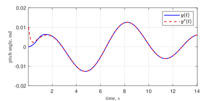
Figure 1: Responses of the output $y(t)$ and $y^{*}(t)$ (Case (i)).

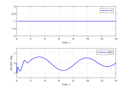
Figure 2: Evolutions of the tuning gain $\sigma$ and input $u(t)$ (Case (i)).

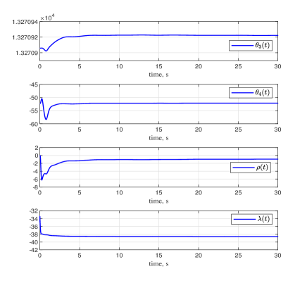
Figure 3: Evolutions of part of parameters in $\Theta(t)$ (Case (i)).

For Case (ii), the response of the system output is shown in Fig. 4. The evolutions of the tuning gain $\sigma$ and input $u(t)$ is depicted in Fig. 5. The evolutions of a subset of parameters in $\Theta(t)$ is shown in Fig. 6. As can be seen from Figs. 1 and 4, compared with that of Case(i), the transient response of the output tracking of Case (ii) has a longer rise time and larger overshoot. This phenomenon is primarily due to the incorrect initial estimation of the sign of $k_{p}$. Recall that $\theta_{4}^{*}=1/k_{p}$, $\lambda^{*}=1/k_{p}$, and $\rho^{*}={k_{p}}$, with their signs being consistent with that of $k_{p}$. However, as depicted in Fig. 6, the signs of $\theta_{4}(t)$, $\lambda(t)$, and $\rho(t)$ may not be consistent with that of $k_{p}$. Nevertheless, the proposed adaptive control scheme can still meet the control objective. The incorrect estimation of the sign of $k_{p}$ can be compensated by automatically adjusting the tuning gain $\sigma$. For instance, even if the sign of $\rho(t)$ is positive, which is opposite to that of $k_{p}$, any potential negative impact on the closed-loop system is avoided by automatically setting $\sigma$ to zero.

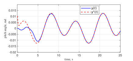
Figure 4: Responses of the output $y(t)$ and $y^{*}(t)$ (Case (ii)).

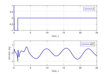
Figure 5: Evolutions of the tuning gain $\sigma$ and input $u(t)$ (Case (ii)).

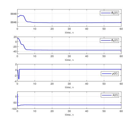
Figure 6: Evolutions of parameters in $\Theta(t)$ (Case (ii)).

The above results demonstrate that the adaptive control scheme proposed in this paper ensures system stability and asymptotic output tracking without requiring any prior knowledge of the high-frequency gain. Meanwhile, the adaptive control law exhibits no singularity or high-gain issues. Moreover, the parameter estimates converge to some constants, and thus the persistent switching issue is avoided.

V Conclusion

This paper presents a new singularity-free MRAC scheme with piecewise constant tuning gain, addressing the unknown high-frequency gain problem in spite of lacking any prior knowledge about high-frequency gain or additional design conditions. The proposed scheme avoids the drawbacks of Nussbaum and multiple-model approaches, which necessitate persistent switching or repeated parameter estimation to handle unknown high-frequency gains, while guaranteeing stability and achieving asymptotic output tracking of the closed-loop system. Specifically, our scheme transforms the estimation error equation into a linear regression form, enabled by a modified MRAC law we developed. This is a key departure from traditional MRAC systems, where the equation for estimating the error takes the form of a bilinear regression. The utilizing of linear regression form simplifies the adaptive control process, which allows for the direct estimation of all unknown parameters. Meanwhile, our scheme designs a piecewise constant tuning gain driven by the least-squares-based parameter update law. This tuning gain ensures that a modified MRAC law we developed achieves the desired control performance with a limited number of adjustments. Finally, our scheme is applied to an aircraft control system, and simulation results demonstrate its effectiveness. Future studies will further extend the proposed adaptive control scheme to multi-input and multi-output systems and relax the design constraints on the unknown high-frequency gain matrix.

Appendix A Two useful lemmas

The following section introduces two lemmas utilized in the proof of Theorem 1.

Lemma 3

([25]) For any vectors $\varpi(t)\in\mathbb{R}^{n}$ and $\xi(t)\in\mathbb{R}^{n}$, if $G_{m}(s)=c_{m}(sI-A)^{-1}b_{m}$ is the minimal realization of a proper transfer function, the following equation holds

$$\varpi^{T}(t)G_{m}(s)[\xi](t)-G_{m}(s)[\varpi^{T}\xi](t)=$$

$$c_{m}(sI-A)^{-1}[(sI-A)^{-1}b_{m}[\xi^{T}](t)\dot{\varpi}](t),$$ (46)

where $\dot{\varpi}(t)$ is the first-time derivative of $\varpi(t)$.

Lemma 4

([25]) Define some notation: $c$ denotes a signal bound; $\kappa$ and $\varrho$ denote generic $L^{2}\cap L^{\infty}$ functions with $\varrho$ asymptotically approaching zero as $t\to\infty$; $\|x\|_{t}$ denotes the norm $\sup_{q\leq t}\max_{1\leq i\leq n}|x_{i}(q)|$ with $x(t)=[x_{1}(t),...,x_{n}(t)]^{T}\in\mathbb{R}^{n}$ being a finite-dimensional vector; and $L^{\infty e}$ denotes the set $\{g(t)~{}|~{}\forall d<\infty,g_{d}(t)\in L^{\infty}\}$, for any function $g(t)$ with $g_{d}(t)=g(t),t\leq d$, and otherwise, $g_{d}(t)=0$. Then, the following results hold

• For a system characterized by $y(t)=G(s)[u](t)$ where $G(s)$ is a strictly proper and stable transfer function, the inequality $\|y\|_{t}\leq\varrho\|v\|_{t}+\varrho$ is satisfied if $\|u\|_{t}\leq\kappa\|v\|_{t}+\kappa$.

• For a system characterized by $y(t)=G(s)[u](t)$ where $G(s)$ is a proper and minimum phase transfer function, the inequality $\|u\|_{t}\leq c\|y\|_{t}+c$ is satisfied if $u$ and $\dot{u}$ belong to $L^{\infty e}$, and $\|\dot{u}\|_{t}\leq c\|u\|_{t}+c$.

References

- [1] A. Astolfi, D. Karagiannis, and R. Ortega, Nonlinear and Adaptive Control with Applications, Springer, London, 2008.
- [2] M. Böhm, M. A. Demetriou, S. Reich, and I. G. Rosen, Model reference adaptive control of distributed parameter systems, SIAM J. Control Optim., 36 (1998), pp. 33–81.
- [3] L. Eugene, W. Kevin, and D. Howe, Robust and Adaptive Control with Aerospace Applications, Springer, London, 2013.
- [4] G. F. Franklin, J. D. Powell, A. Emami-Naeini, and J. D. Powell, Feedback Control of Dynamic Systems, Prentice Hall, Upper Saddle River, 2002.
- [5] G. C. Goodwin and K. S. Sin, Adaptive Filtering Prediction and Control, Dover Publications, Mineola, 2014.
- [6] X. Guo, C. Wang, Z. Dong, and Z. Ding, Adaptive containment control for heterogeneous mimo nonlinear multiagent systems with unknown direction actuator faults, IEEE Trans. Automat. Control, 68 (2023), pp. 5783–5790.
- [7] A. Hastir, J. J. Winkin, and D. Dochain, Funnel control for a class of nonlinear infinite-dimensional systems, Automatica J. IFAC, 152 (2023), p. 110964.
- [8] W. Hong, G. Tao, H. Wang, and C. Wang, Traffic signal control with adaptive online-learning scheme using multiple-model neural networks, IEEE Trans. Neural Netw. Learn. Syst., 34 (2022), pp. 7838–7850.
- [9] C.-C. Hua, H. Li, K. Li, and P. Ning, Adaptive prescribed-time stabilization of uncertain nonlinear systems with unknown control directions, IEEE Trans. Automat. Control, 69 (2024), pp. 3968–3974.
- [10] P. A. Ioannou and J. Sun, Robust Adaptive Control, Prentice Hall, Upper Saddle River, 1996.
- [11] Y. Jiang, W. Gao, C. Chen, T. Chai, and F. L. Lewis, Adaptive optimal control of linear discrete-time networked control systems with two-channel stochastic dropouts, SIAM J. Control Optim., 61 (2023), pp. 3183–3208.
- [12] M. Krstic, I. Kanellakopoulos, and P. Kokotovic, Nonlinear and Adaptive Control Design, John Wiley & Sons, New York, 1995.
- [13] I. D. Landau, R. Lozano, M. M’Saad, and A. Karimi, Adaptive Control: Algorithms, Analysis and Applications, Springer, London, 2011.
- [14] X. Li and Z. Hou, Robust adaptive iterative learning control for a generic class of uncertain non-square mimo systems, IEEE Trans. Automat. Control, 69 (2024), pp. 2721–2728.
- [15] R. Lozanoleal, J. Collado, and S. Mondie, Model reference robust adaptive control without a priori knowledge of the high freqency gain, IEEE Trans. Automat. Control, 35 (1990), pp. 71–78.
- [16] M. Lv, Z. Chen, B. De Schutter, and S. Baldi, Prescribed-performance tracking for high-power nonlinear dynamics with time-varying unknown control coefficients, IEEE Trans. Automat. Control, 146 (2022), p. 110584.
- [17] Y. Ma, G. Tao, B. Jiang, and Y. Cheng, Multiple-model adaptive control for spacecraft under sign errors in actuator response, J. Guid. Control Dyn., 39 (2016), pp. 628–641.
- [18] S. M. Mousavi and M. Guay, An observer-based extremum seeking controller design for a class of second-order nonlinear systems, IEEE Control Syst. Lett., 8 (2024), pp. 1913–1918.
- [19] K. Narendra and J. Balakrishnan, Improving transient response of adaptive control systems using multiple models and switching, IEEE Trans. Automat. Control, 39 (1994), pp. 1861–1866.
- [20] F. Navas, V. Milanes, C. Flores, and F. Nashashibi, Multi-model adaptive control for CACC applications, IEEE Trans. Intell. Transp. Syst., 22 (2021), pp. 1206–1216.
- [21] N. T. Nguyen and N. T. Nguyen, Model-Reference Adaptive Control, Springer, London, 2018.
- [22] R. D. Nussbaum, Some remarks on a conjecture in parameter adaptive control, Systems Control Lett., 3 (1983), pp. 243–246.
- [23] G. Pin, A. Serrani, and Y. Wang, Parameter-dependent input normalization: Direct-adaptive control with uncertain control direction, in Proceeding: IEEE 61st Conference on Decision and Control, 2022, pp. 2674–2680.
- [24] M. Radenkovic and M. Tadi, Self-tuning consensus on directed graphs in the case of unknown control directions, SIAM J. Control Optim., 54 (2016), pp. 2339–2353.
- [25] S. Sastry and M. Bodson, Adaptive Control: Stability, Convergence and Robustness, Prentice Hall, Upper Saddle River, 1989.
- [26] S. S. Sastry and A. Isidori, Adaptive control of linearizable systems, IEEE Trans. Automat. Control, 34 (1989), pp. 1123–1131.
- [27] A. Scheinker and M. Krstic, Minimum-seeking for clfs: Universal semiglobally stabilizing feedback under unknown control directions, IEEE Trans. Automat. Control, 58 (2012), pp. 1107–1122.
- [28] G. Tao, Adaptive Control Design and Analysis, John Wiley & Sons, Hoboken, 2003.
- [29] G. Tao and M. Suresh, Adaptive Control of Systems with Actuator Failures, Springer, London, 2001.
- [30] C. Wang, C. Wen, and L. Guo, Multivariable adaptive control with unknown signs of the high-frequency gain matrix using novel nussbaum functions, Automatica, 111 (2020), p. 108618.
- [31] L. Wang and C. M. Kellett, Robust i&i adaptive tracking control of systems with nonlinear parameterization: An iss perspective, Automatica, 158 (2023), p. 111273.
- [32] L. Wang, R. Ortega, and A. Bobtsov, Observability is sufficient for the design of globally exponentially stable state observers for state-affine nonlinear systems, Automatica J. IFAC, 149 (2023), p. 110838.
- [33] Y. Wang and Y. Liu, Global output-feedback control by exploiting high-gain dynamic-compensation mechanisms, SIAM J. Control Optim., 62 (2024), pp. 1122–1151.
- [34] Y. Xu, Y. Zhang, and J.-F. Zhang, Singularity-free adaptive control of discrete-time linear systems without prior knowledge of the high-frequency gain, Automatica J. IFAC, 165 (2024), p. 111657.
- [35] L. Yan, L. Hsu, R. R. Costa, and F. Lizarralde, A variable structure model reference robust control without a prior knowledge of high frequency gain sign, Automatica J. IFAC, 44 (2008), pp. 1036–1044.
- [36] X. Yan and Y. Liu, Global practical tracking for high-order uncertain nonlinear systems with unknown control directions, SIAM J. Control Optim., 48 (2010), pp. 4453–4473.
- [37] D. Yue, S. Baldi, J. Cao, and B. D. Schutter, Model reference adaptive stabilizing control with application to leaderless consensus, IEEE Trans. Automat. Control, 69 (2024), pp. 2052–2059.
- [38] J. F. Zhang and P. E. Caines, Adaptive control via a simple switching algorithm, SIAM J. Control Optim., 34 (1996), pp. 365–388.
- [39] J.-X. Zhang and G.-H. Yang, Prescribed performance fault-tolerant control of uncertain nonlinear systems with unknown control directions, IEEE Trans. Automat. Control, 62 (2017), pp. 6529–6535.
- [40] Y. Zhang and J.-F. Zhang, A quantized output feedback mrac scheme for discrete-time linear systems, Automatica J. IFAC, 145 (2022), p. 110575.