CVA Sensitivities, Hedging and Risk

Abstract

We present a unified framework for computing CVA sensitivities, hedging the CVA, and assessing CVA risk, using probabilistic machine learning meant as refined regression tools on simulated data, validatable by low-cost companion Monte Carlo procedures. Various notions of sensitivities are introduced and benchmarked numerically. We identify the sensitivities representing the best practical trade-offs in downstream tasks including CVA hedging and risk assessment.

Keywords: learning on simulated data; sensitivities; CVA pricing, hedging, and risk; neural networks; value-at-risk and expected shortfall; economic capital; model risk.

1 Introduction

This work illustrates the potential of probabilistic machine learning for pricing and Greeking applications, in the challenging context of CVA computations. By probabilistic machine learning we mean machine learning as refined regression tools on simulated data. Probabilistic machine learning for CVA pricing was introduced in Abbas-Turki, Crépey, and Saadeddine (2023). Here we extend our approach to encompass CVA sensitivities and risk. The fact that probabilistic machine learning is performed on simulated data, which can be augmented at will, does not mean that there are no related data issues. As always with machine learning, the quality of the data is the first driver of the success of the approach. The variance of the training loss may be high and jeopardize the potential of a learning approach. This was first encountered in the CVA granular defaults pricing setup of Abbas-Turki et al. (2023) due to the scarcity of the default events compared with the diffusive scale of the risk factors in the model. Switching from prices to sensitivities in this paper is another case of increased variance. But with probabilistic machine learning we can also develop suitable variance reduction tools, namely oversimulation of defaults in Abbas-Turki et al. (2023) and common random numbers in this work. Another distinguishing feature of probabilistic machine learning, which is key for regulated banking applications, is the possibility to assess the quality of a predictor by means of low-cost companion Monte Carlo procedures.

1.1 Outline of the Paper and Generalities

Section 2 introduces different variants of bump sensitivities, benchmarked numerically in a CVA setup in Section 3. Section 4 shows how a conditional (e.g. future) CVA can be learned from simulated data (pricing model parameters and paths and financial derivative cash flows), both in a baseline calibrated setup and in an enriched setup also accounting for recalibration model shifts. Sections 5 and 6 develop a framework for internal modeling of CVA and/or counterparty default risks, entailing various notions of CVA sensitivities. Section 7 concludes as for which kind of sensitivity and numerical scheme provide the best practical trade-off for various downstream tasks including CVA hedging and risk assessment.

A vector of partial derivatives with respect to $x$ is denoted by $\partial_{x}$ (or $\cdot^{\prime}$ when $x$ is clear from the context). All equations are written using the risk-free asset as a numéraire and are stated under the probability measure which is the blend of physical and pricing measures advocated for XVA computations in Albanese, Crépey, Hoskinson, and Saadeddine (2021, Remark 2.3), with related expectation operator denoted below by $\mathbb{E}$. All cash flows are assumed square integrable. Some standing notation is listed in Table 1.

$\rho$ ee ee	model parameters, i.e. exogenous model parameters $\epsilon$ and initial conditions of model risk factors	$Y$ ee ee	CVA diffusive risk factor process with initial condition $y$ (if constant) or $\iota$ (if randomized)
$\varrho$	randomization of $\rho$	$X$	default indicator processes of clients
$\omega$ ee	stochastic drivers (e.g. Brownian paths)	$Z$ ee	market price process, with initial condition $z_{0}$
$\rho_{0}$	calibrated value of $\rho$	$\xi(\rho;\omega)$	product payoff
$\bar{\cdot}$	$2\rho_{0}-\cdot$	$\Pi_{0}$	$\mathbb{E}\xi(\rho)$
$\cdot^{\theta}$	neural net function with parameters $\theta$	$\varsigma(\rho;\omega)$	$\xi(\rho;\omega)-\xi(\bar{\rho};\omega)$
$q$	number of market instruments	$\Sigma_{0}(\rho)$	$\mathbb{E}\varsigma(\rho)$
$m$ ee	number of Monte Carlo paths of the pricing model	$\Delta$ ee	CVA hedging ratio or linear coefficients of a CVA proxy
$p$ ee	number of model parameters, i.e. dimension of $\rho$	$\Gamma$ ee	diagonal quadratic coefficients of a CVA proxy

Table 1: Standing notation.

All neural network trainings are done using the PyTorch module and the Adam optimizer. Linear regressions are implemented using a truncated singular value decomposition (SVD) approach. Unless explicitly stated, we always include a ridge (i.e. Tikhonov) regularization term in the loss function to stabilize trainings and regressions. Our computations are run on a server with an Intel(R) Xeon(R) Gold 5217 CPU and a Nvidia Tesla V100 GPU.

2 Fast Bump Sensitivities

In this section we consider a time-0 option price $\Pi_{0}(\rho)=\mathbb{E}\xi(\rho),$ where the payoff $\xi(\rho)\equiv\xi(\rho;\omega)$ depends on constant model parameters $\rho$ and (implicitly in the shorthand notation $\xi(\rho)$) on the randomness $\omega$ of the stochastic drivers of the model risk factors with respect to which the expectation is taken above. The model parameters $\rho$ encompass the initial values of the risk factors of the pricing model, as well as all the exogenous (constant, in principle) model parameters, e.g. the value of the volatility in a Black-Scholes model. For each constant $\rho$, the price $\Pi_{0}(\rho)$ can be estimated by Monte Carlo. Our problem in this part is the estimation of the corresponding sensitivities $\partial_{\rho}\Pi_{0}(\rho_{0})$, at a baseline (in practice, calibrated) value $\rho=\rho_{0}$ of the model parameters. Such sensitivities lie at the core of any related hedging scheme for the option. They are also key in many regulatory capital formulas.

Monte Carlo estimation of sensitivities in finance comes along three main streams (Crépey, 2013, Section 6.6): (i) differentiation of the density of the underlying process via integration by parts or more general Malliavin calculus techniques, assuming some regularity of this process; (ii) cash flows differentiation, assuming their differentiability, in chain rule with the stochastic flow of the underlying process; (iii) Monte Carlo finite differences, biased but generic, which are the Monte Carlo version of the industry standard bump sensitivities. But (i) suffers from intrinsic variance issues. In contemporary technology, (ii) appeals to adjoint algorithmic differentiation (AAD). A randomized version of this approach is provided by Sections 5.3–5.5 of Saadeddine (2022), targeted to model calibration, which requires sensitivities of vanilla options as a function of their model parameters. However, the embedded AAD layer can quickly represent important implementation and memory costs on complex pricing problems at the portfolio level such as CVA computations: see Capriotti, Jiang, and Macrina (2017). Such an AAD Greeking approach becomes nearly unfeasible in the case of pricing problems embedding numerical optimization subroutines, e.g. the training of the conditional risk measures embedded in the refined CVA and higher-order XVA metrics of Albanese et al. (2021) (with Picard iterations) or Abbas-Turki, Crépey, Li, and Saadeddine (2024) (explicit scheme without Picard iterations).

2.1 Common Random Numbers

Under the approach (iii), first-order pointwise bump sensitivities are computed by relaunching the Monte Carlo pricing engine with common random numbers $\omega$ for values bumped by $\pm 1\%$ (typically and in relative terms) of each risk factor and/or model parameter of interest, then taking the accordingly normalized difference between the corresponding $\Pi_{0}(\rho)$ and $\Pi_{0}(\bar{\rho})$, where $\bar{\cdot}$ means symmetrization with respect to $\rho_{0}$, so

$$\begin{aligned} \frac{\rho+\bar{\rho}}{2}=\rho_{0},\;\mbox{i.e. }\bar{\rho}=2\rho_{0}-\rho.\end{aligned}$$ (1)

This approach requires two Monte Carlo simulation runs per sensitivity, making it a robust but heavy procedure, which we try to accelerate by various means in what follows.

A predictor $\Pi_{0}^{\theta}(\rho)\approx\Pi_{0}(\rho)$ for the pricing function around $\rho=\rho_{0}$ within a suitable space of neural nets parameterized by $\theta$ readily leads to an AAD estimate $\partial_{\rho}\Pi_{0}(\rho_{0})\approx\partial_{\rho}\Pi^{\theta}_{0}(\rho_{0})$ for the corresponding sensitivities. However, even if ridge regularization may help in this regard, such an estimate, deemed naive AAD hereafter, may be bad as differentiation is not a continuous operator in the supremum norm (in other terms, functions may be arbitrarily close in sup norm but their derivatives may be far from each other). Specifically, let $\mathcal{B}$ denote the space of the Borel measurable functions of $\rho$. The pricing function

$$\begin{aligned} \Pi_{0}(\rho)=\mathbb{E}\xi(\rho)=\mathbb{E}\big{(}\xi(\varrho)\,\big{|}\,\varrho=\rho\big{)}\end{aligned}$$ (2)

(for $\varrho$ randomizing $\rho$ around $\rho_{0}$) can be learned from simulated pairs $(\varrho,\xi(\varrho;\omega))$ based on the representation

$$\begin{aligned} \Pi_{0}(\cdot)=\operatorname*{arg\,min}_{\Phi\in\mathcal{B}}\mathbb{E}\Big{[}\big{(}\xi(\varrho)-\Phi(\varrho)\big{)}^{2}\Big{]}.\end{aligned}$$ (3)

To learn the function $\Pi_{0}(\cdot)$ around $\rho_{0}$, we can replace, in the optimization problem (3), $\mathcal{B}$ by a suitable space of neural nets and $\mathbb{E}$ by a simulated sample mean $\widehat{\mathbb{E}}$, with each “vertical” (time-0) draw of $\varrho$ followed by an “horizontal” (across future times) draw of $\omega$ that is implicit in $\xi(\varrho)\equiv\xi(\varrho;\omega)$. The ensuing minimization problem for the weights $\theta$ of the neural net $\rho\mapsto\Pi^{\theta}_{0}(\rho)\approx\Pi_{0}(\rho)$ is then performed numerically by Adam mini-batch gradient descent. The corresponding sensitivities $\partial_{\rho}\Pi^{\theta}_{0}(\rho_{0})$ are retrievable by AAD at negligible additional cost. However, as emphasized above, the ensuing naive AAD sensitivities $\partial_{\rho}\Pi^{\theta}_{0}$ may be a poor estimate of $\partial_{\rho}\Pi_{0}$.

In this learning setup, the corresponding instability reflects a variance issue. In order to cope with the increased variance due to the switch from prices to sensitivities, a useful trick is to introduce $\varsigma(\rho;\omega):=\xi(\rho;\omega)-\xi(\bar{\rho};\omega)$ (cf. (1)). We can then learn the sensitivity (in the sense here of finite differences) function $\rho\mapsto\Sigma_{0}(\rho):=\mathbb{E}\varsigma(\rho)$, which satisfies by linearity and chain rule (as $\bar{\rho}=2\rho_{0}-\rho$)

$$\begin{aligned} \Sigma^{\prime}_{0}(\rho)=\Pi^{\prime}_{0}(\rho)+\Pi^{\prime}_{0}(\bar{\rho})\mbox{, in particular }\partial_{\rho}\Sigma_{0}(\rho_{0})=2\partial_{\rho}\Pi_{0}(\rho_{0}).\end{aligned}$$ (4)

For learning the function $\Sigma_{0}(\cdot)$ locally around $\rho_{0}$, with $\varrho$ randomizing $\rho$ as above, we rely on the representation $\Sigma_{0}(\rho)=\mathbb{E}\big{(}\varsigma(\varrho)\,\big{|}\,\varrho=\rho\big{)},$ i.e.

$$\begin{aligned} \Sigma_{0}(\cdot)=\operatorname*{arg\,min}_{\Phi\in\mathcal{B}}\mathbb{E}\Big{[}\big{(}\varsigma(\varrho)-\Phi(\varrho)\big{)}^{2}\Big{]}.\end{aligned}$$ (5)

Then we replace, in the optimization problem (5), $\mathcal{B}$ by a linear hypothesis space $\Sigma^{\theta}_{0}(\rho)=\theta^{\top}(\rho-\rho_{0})$ (noting that $\Sigma_{0}(\rho_{0})=0$) and $\mathbb{E}$ by a simulated sample mean $\widehat{\mathbb{E}}$, with again each vertical draw of $\varrho$ followed by one horizontal draw of $\omega$ that is implicit in $\varsigma(\varrho)$. This results in a linear least-squares problem for the weights $\theta$, solved by SVD. The estimated weights $\theta/2$ are our linear bump sensitivities estimate for $\frac{1}{2}\partial_{\rho}\Sigma_{0}(\rho_{0})=\partial_{\rho}\Pi_{0}(\rho_{0})$. These sensitivity estimates are the slope coefficients of a multilinear regression, for which confidence intervals CI scaling in $1/\sqrt{|\mbox{sample size}|}$ are available (Matloff, 2017, Section 2.12.11). The use of each drawn set of model parameters $\varrho$ twice, also via $\bar{\varrho}$ with a common $\omega$ in $\varsigma(\varrho;\omega)=\xi(\varrho;\omega)-\xi(\bar{\varrho};\omega)$, is a common random numbers variance reduction technique as in (iii) above. For well-chosen distributions of the randomization $\varrho$ of $\rho$, this approach results in much more accurate sensitivities than the naive AAD approach. For simple parametric distributions of $\varrho$, the covariance matrix that appears in the regression for the first-order sensitivities is known and invertible in closed form, which reduces the linear regression (implemented without ridge regularization in this analytical case) to a standard Monte Carlo and a more robust CI. Nonlinear hypothesis spaces of neural networks trained the way described after (3) (just replacing $\xi(\varrho)$ and $\partial_{\rho}\Pi^{\theta}_{0}(\rho_{0})$ there by $\varsigma(\varrho)$ and $\partial_{\rho}\Sigma^{\theta}_{0}(\rho_{0})$ here) can also be used instead of the above linear model for $\Sigma_{0}(\rho)$. The AAD bump sensitivities are then obtained as the halved AAD sensitivities of the trained (no longer linear) network $\rho\mapsto\partial_{\rho}\Sigma^{\theta}_{0}$ at $\rho_{0}$ (but we lose the confidence interval CI in this case). Similar ideas can be applied to higher order sensitivities, using e.g. $\xi(\rho;\omega)-2\xi(\rho_{0};\omega)+\xi(\bar{\rho};\omega)$ instead of $\varsigma(\rho;\omega)=\xi(\rho;\omega)-\xi(\bar{\rho};\omega)$ to capture diagonal gammas. However, higher order means even more variance. Moreover, the Jacobian trick of Section 2.3 to convert model into market sensitivities is only workable for first-order sensitivities, hence our focus on the latter in this work.

An important ingredient in successful randomized (linear or AAD) bump sensitivities is the choice of appropriate distributions for $\varrho$. Since different parameters (components of $\rho$) may have very different magnitudes in values and price impact (see e.g. Figure 1 page 1 and Table 2 page 2), a linear regression may not be able to identify the individual effect of each parameter when all are bumped simultaneously. To address this issue, we divide the parameters into groups. The $m$ simulated paths of the pricing model are then partitioned into blocks of paths such that only one group of parameters is bumped in each subset. In addition to this, one can use different distributions for each group or even for each parameter. Notably, we have observed numerically that slightly noiser distributions yield better sensitivities estimates for volatility-related parameters.

input : A (calibrated) baseline $\rho_{0}$ for the initial conditions of all risk factors and for the exogenous parameters of the pricing model, a number $m$ of pricing model paths.

output : Estimated sensitivities $\theta/2$ (linear case) or $\frac{1}{2}\partial_{\rho}\Sigma^{\theta}_{0}(\rho_{0})$ (more generally) $\approx\partial_{\rho}\Pi_{0}(\rho_{0})$.

1 Draw $m$ i.i.d. bumped model parameters $\rho_{j}$ from some distribution randomizing $\rho$ around $\rho_{0}$, e.g. $\mathcal{N}\Big{(}\rho_{0},\mathrm{diag}\left(\sigma^{2}\rho_{0}\odot\rho_{0}\right)\Big{)}$ with $\sigma=1\%,3\%,5\%$ or, in the case of smart bump sensitivities, $\rho_{j}=\rho_{0}$ bumped by $1\%$ on its $\left\lfloor\frac{jp}{m}\right\rfloor$-th component

2Draw $m$ i.i.d. stochastic drivers $\omega$ parameters $\{\omega_{1},\dots,\omega_{m}\}$

3for $(\rho,\omega)\in(\rho_{1},\omega_{1})\,..\,(\rho_{1},\omega_{m})$ do

4       Compute the payoffs $\xi(\rho;\omega)$ and $\xi(\bar{\rho};\omega)$, where $\frac{\rho+\bar{\rho}}{2}=\rho_{0}$

5       Compute $\varsigma(\rho;\omega)=\xi(\rho;\omega)-\xi(\bar{\rho};\omega)$

6 end for

7if AAD bump sensitivities then

8       Train a neural network $\Sigma_{0}^{\theta}(\rho)$ to regress $(\varsigma(\rho_{1}),\dots,\varsigma(\rho_{m}))$ against $(\rho_{1},,\dots,\rho_{m})$

9       Retrieve $\partial_{\rho}\Sigma_{0}^{\theta}(\rho)$ by AAD and divide the obtained gradient by two for obtaining the AAD bump sensitivities.

10 else if Linear bump sensitivities then

11       Regress linearly (without intercept) $(\varsigma(\rho_{1}),\dots,\varsigma(\rho_{m}))$ against $(\rho_{1}-\rho_{0},\dots,\rho_{m}-\rho_{0})$ by SVD

12       Divide the regression coefficients $\theta$ by two for obtaining the linear bump sensitivities

13 else if Smart bump sensitivities then

14       Compute each sensitivity by dividing the average of $\varsigma$ over each block of size $m/p$ by two times the corresponding bump size

15 end if

Algorithm 1 Fast bump sensitivities.

In addition to the above, we will also compute benchmark bump sensitivities as per (iii) in the above, obtained on the basis of $p$ Monte Carlo repricings with $m$ common random numbers $\omega$ and relative variations of $\pm 1\%$ of one model parameter in each Monte Carlo run, as well smart bump sensitivities, similar but only using $m/p$ paths each, where $p$ is the number of model parameters (dimension of $\rho$). Hence the time of computing all the smart bump sensitivities is of the same order of magnitude as the one of retrieving the linear bump sensitivities, which is also roughly the time of pricing $\Pi_{0}(\rho_{0})$ by Monte Carlo with $m$ paths. More precisely, each smart bump sensitivity uses $m/p$ paths of a Monte Carlo simulation run with $m$ paths as a whole. This is significantly more efficient than doing $p$ Monte Carlo runs of size $m/p$ each, especially in the GPU simulation environment of our CVA computations later below. Note that such smart bump sensitivities are also a special case of linear bump sensitivities with block simulation trick, for blocks of size $m/p$ and deterministic bumps of relative size 1% on one and only one model parameter in each block, the linear regression degenerating in this case to a local sample mean over the $m/p$ paths of each block: see Algorithm 1, which summarizes the above procedures for various fast bump sensitivities.

2.2 Basket Black-Scholes Example

Let us consider a European call on the geometric average of $d$ Black-Scholes assets, aiming for the corresponding deltas, vegas, and (diagonal) gammas, which are known analytically in this lognormal setup. Regarding the above block simulation trick, the time-0 values of the assets are bumped in half of the paths, while the volatilities are bumped in the other half. We study two cases, with $d=3$ and $10$ and, respectively $m=10^{5}$ and $m=5\times 10^{5}$ simulated Black-Scholes paths. In the $d=3$ case, we implement all the fast bump approaches of Algorithm 1 and the naive AAD approach described after (3). The learning of the gammas is also reported in this low-dimensional experiment. In the $d=10$ case, we skip the naive AAD approach as well as all the learned gamma results because of their poor performance. The hypothesis space used in all the AAD approaches is a vanilla multi-layer perceptron with two hidden layers and softplus activation functions.

The error bars in Figure 1 page 1 represent our $95\%$ confidence intervals (CI) for the linear bump sensitivities. Regarding the AAD bump approach, we train the neural network 100 times with different initializations to also get a 95% confidence interval, in a meaning weaker than CI though: as the data is not resampled in each run, the AAD confidence intervals (CI^♭) can only account for the randomness in training, not for the one of the simulated data. The upper plots of Figure 1 show the inaccuracy of the naive AAD sensitivities. The fast bump approaches consistently estimate deltas, but vegas and gammas appear to be more challenging. This is due to greater variance in the case of gammas, whereas in the case of vegas, the collusion between the noise of the random volatility coefficient and the one of the Brownian drivers $\omega$ makes the learning task more difficult. As should be, the CIs of the linear and smart bump sensitivities contain nearly all the exact sensitivities. This is also mostly the case for the CI^♭s of the AAD bump sensitivities, but in their case this comes without theoretical guarantee. The benchmark bump sensitivities are exact with 2 significant digits (at least for deltas and vegas) in this Black-Scholes setup. They would be visually indistinguishable of the exact sensitivities if we added them on the graphs of Figure 1. The time of computing the smart bump sensitivities is of the same order of magnitude as the one of retrieving the linear bump sensitivities, with also similar accuracy as demonstrated in Figure 3(a) page 3, where both ratios between running times and errors of the linear and smart bump sensitivities with respect to the benchmark bump sensitivities stay close to each other. The complexities, describing how long it would take for each algorithm to achieve a relative error in the Black-Scholes case (or standard error in the CVA case) of 1%, are not significantly different for the linear, smart and benchmark bump sensitivities, for most of $p$; otherwise the smart ones beat by a small margin the linear ones, themselves a bit worse than the benchmark ones. The grey dashed lines in the right panels indicate the $p^{2}$ scaling of complexities expected for the benchmark bump sensitivities, which involve $2p$ simulation runs in dimension $\Theta(p)$ (the number of risk factors in the pricing model).

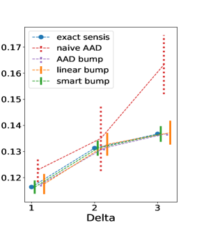
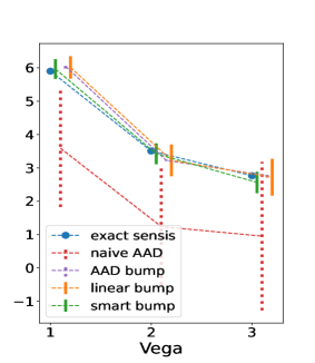
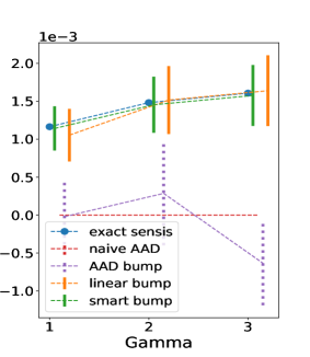
(a) $d=3$ and $m=10^{5}$ paths.

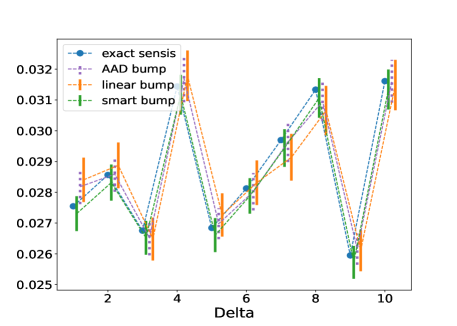
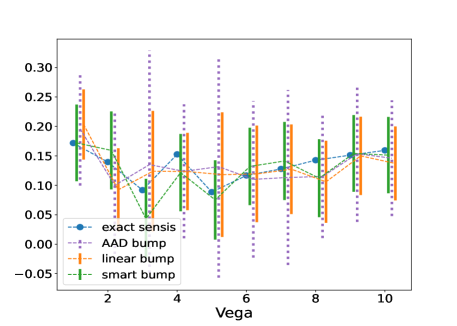
(b) $d=10$ and $m=5\times 10^{5}$ paths.

Figure 1: Multi-asset geometric average call sensitivities on 3 (a) and 10 (b) independent Black-Scholes assets. The error bars represent confidence intervals CI or CI^♭, in dotted lines regarding the latter, which only reflect a training noise.

In general, we observed that in high dimension the linear and smart bump sensitivities tend to be more stable and reliable than the AAD bump sensitivities. Hence we forget AAD bump sensitivities hereafter.

2.3 From Model to Market Sensitivities

The sensitivities $\partial_{\rho}\Pi_{0}(\rho_{0})$ are sensitivities to model parameters. Practical hedging schemes require sensitivities to calibrated prices of hedging instruments. Hence, for hedging purposes, our sensitivities must be mapped to hedging ratios in market instruments. This can be done via the implicit function theorem, the way explained in Henrard (2011), Savine (2018), and Antonov et al. (2018). In a nutshell, assume that, given market prices $z\in\mathbb{R}^{q}$ of suitable calibration (hedging) assets, the corresponding pricing model parameters $\rho(z)$ are obtained by a calibration procedure of the form

$$\rho(z)\in\underset{\rho\in\mathbb{R}^{p}}{\mathrm{argmin}}\,cal\mbox{-}err\left(z,\rho\right),$$ (6)

where $cal\mbox{-}err\left(z,\rho\right)$ quantifies the mean square error between the market prices $z$ of the calibration instruments and their prices in the pricing model with parameters $\rho$. Note that, in practice, not all the pricing parameters are obtained via a minimization as in (6): some of them are bootstrapped or even directly observed on the market, see Savine (2018) for a more detailed presentation and Section 3.1 for an example.

Assume $cal\mbox{-}err$ of class $\mathcal{C}^{2}$ in $\rho$. Let $\rho(z_{0})=\rho_{0}$ be a solution of (6) associated with a particular $z=z_{0}$, hence $\partial_{\rho}cal\mbox{-}err(z_{0},\rho_{0})=0$. Denote by $\partial^{2}_{\rho,\rho}cal\mbox{-}err$ the Hessian matrix of $cal\mbox{-}err$ with respect to $\rho$ and assume that $\partial^{2}_{\rho,\rho}cal\mbox{-}err(z_{0},\rho_{0})$ is invertible. Then, by the implicit function theorem applied to the function $\partial_{\rho}cal\mbox{-}err$ of $(z,\rho)$, there exists an open neighborhood $\mathcal{O}\in\mathbb{R}^{q}$ of $z_{0}$ on which (6) uniquely defines a function $\mathcal{O}\ni z\mapsto\rho(z)$, i.e. $\partial_{\rho}cal\mbox{-}err(z,\rho(z))=0$ for all $z\in\mathcal{O}$. Moreover, if $\rho$ is in $\mathcal{C}^{1}\left(\mathcal{O};\mathbb{R}^{p}\right)$, then

$$\begin{aligned} \partial_{z}\rho(z)=-\Big{(}\partial^{2}_{\rho,\rho}cal\mbox{-}err(z,\rho(z))\Big{)}^{-1}\Big{(}\partial^{2}_{\rho,z}cal\mbox{-}err(z,\rho(z))\Big{)},\;\mbox{for all $z\in\mathcal{O}$},\end{aligned}$$

where we assume that the matrix of all the second derivatives of $cal\mbox{-}err$ with respect to one component in $\rho$ and one component in $z$, denoted by $\partial^{2}_{\rho,z}cal\mbox{-}err$, exists. From there, the chain rule

$$\begin{aligned} &(\partial_{z}\Pi_{0}(z))^{\top}=\Big{(}\partial_{\rho}\Pi_{0}(\rho(z))\Big{)}^{\top}\partial_{z}\rho(z)\\ &=-\Big{(}\partial_{\rho}\Pi_{0}(\rho(z))\Big{)}^{\top}\Big{(}\partial^{2}_{\rho,\rho}cal\mbox{-}err(z,\rho(z))\Big{)}^{-1}\Big{(}\partial^{2}_{\rho,z}cal\mbox{-}err(z,\rho(z))\Big{)},\;\mbox{for $z\in\mathcal{O}$},\end{aligned}$$ (7)

allows deducing the market sensitivities $\partial_{z}\Pi_{0}$ from the model sensitivities $\partial_{\rho}\Pi_{0}$. When heavy Monte Carlo (such as CVA) pricing tasks are involved in the $\partial_{\rho}\Pi_{0}$ computations, the time of computing $\partial_{z}\Pi_{0}$ through (7) is dominated by the time of computing $\partial_{\rho}\Pi_{0}$.

Another way to compute market bump sensitivities is to bump each target calibration price and recompute the price $\Pi_{0}$ for pricing model parameters $\rho$ recalibrated to each bumped calibrated data set. This direct approach does not need Jacobian transformations and it is also amenable to second-order sensitivities. However, accounting for curves and surfaces of hedging assets, there may be much more market sensitivities than model sensitivities (as in our use case of Section 3.1). Moreover, direct market sensitivities require not only intensive repricings but also model recalibrations, as many as targeted market sensitivities. The direct approach is therefore typically much heavier than the one based on model bump sensitivities followed by Jacobian transformations. We therefore forget direct market bump sensitivities hereafter: by market bump sensitivities, we mean from now on (first-order) bump sensitivities with respect to model parameters, transformed to the corresponding first-order market sensitivities via (7).

3 Credit Valuation Adjustment and Its Bump Sensitivities

In the above Black-Scholes setup, bump sensitivities are useless because the exact Greeking formulas are also faster. We now switch to CVA computations in the role of $\Pi$ before, for which pricing and Greeking can only be achieved by intensive Monte Carlo simulations implemented on GPU. Since we are also interested in the risk of CVA fluctuations (if unhedged, or of fluctuations of a hedged CVA position more generally), we now consider the targeted price $\Pi$ (CVA from now on) as a process. We denote by $\mathrm{MtM}^{c}$, the counterparty-risk-free valuation of the portfolio of the bank with its client $c$; $\tau_{c}$, the client $c$’s default time, with intensity process $\gamma^{c}$; $X$, with $X_{0}\equiv 0$ (componentwise), the vector of the default indicator processes of the clients of the bank; $Y$, a diffusive vector process of model risk factors such that each ${\rm MtM}^{c}_{t}$ and $\gamma^{c}_{t}$ is a measurable function of $(t,Y_{t})$, for $t\geq 0$ (in the case of credit derivatives with the client $c$, ${\rm MtM}^{c}_{s}$ would also depend on $X_{t}$, which can be accommodated at no harm in our setup). The exogenous model parameters are denoted by $\epsilon$. Let the baseline $\rho_{0}=(y_{0},\epsilon_{0})$ denote a calibrated value of $(y,\epsilon)$, where $y$ is used for referring to the initial condition of $Y$, whenever assumed constant. Let $\iota$ denote an initial condition for $Y$ randomized around its baseline $y_{0}$, $\varepsilon$ be likewise a randomization of $\epsilon$ around its baseline $\epsilon_{0}$, and $\varrho_{t}=(Y_{t},\varepsilon),t\geq 0$. Starting from the (random) initial condition $(0,\iota)$, the model $(X,Y)$ is supposed to evolve according to some Markovian dynamics (e.g. the one of Section 3.1) parameterized by $\varepsilon$. This setup allows encompassing in a common formalism:

• the baseline mode of Abbas-Turki et al. (2023, Section 4) where $\varrho_{0}\equiv\rho_{0}$;

• the risk mode where $Y_{0}\equiv y_{0}$;

• the sensis mode, or general $\varrho_{0}$ case, used with an exogenous distribution of $\iota$ in Section 3.1 and with $\iota$ distributed as the diffusive risk factors of the CVA simulation engine in the risk mode at a specified risk horizon in Section 6.

The CVA engine in the baseline mode $\varrho_{0}\equiv\rho_{0}$ was introduced in Abbas-Turki et al. (2023). The risk and sensis mode also incorporating a randomization $\varepsilon$ of the exogenous model parameters $\epsilon$, and of $Y_{0}$ in the sensis mode, are novelties of the present work.

We restrict ourselves to an uncollateralized CVA for notational simplicity. Given $n$ pricing time steps of length $h$ such that $nh=T$, the final maturity of the derivative portfolio of the bank, let, at each $t=ih$,

$$\begin{aligned} &{\rm LGD}_{t}=\sum_{c}\sum_{j=0}^{{i-1}}(\mathrm{MtM}^{c}_{jh})^{+}\mathds{1}_{{jh<\tau_{c}\leq(j+1)h}},\\ &\xi_{t,T}=h\sum_{c}\sum_{j=i}^{{n-1}}({\mathrm{MtM}}^{c}_{jh})^{+}(e^{-\sum_{\imath=i}^{j-1}\gamma^{c}_{\imath}}-e^{-\sum_{\imath=i}^{j}\gamma^{c}_{\imath}})\mathds{1}_{{\left\{\tau_{c}>ih\right\}.}}\end{aligned}$$ (8)

Our computations rely on the following default-based and intensity-based formulations of the (time-discretized) CVA of a bank with clients $c$, at the pricing time $t=ih$ (cf. Abbas-Turki et al. (2023, Eqns. (25)-(27))):

$$\begin{aligned} &{\mathrm{CVA}}_{t}(x,\rho)=\mathbb{E}\Big{[}\underbrace{\sum_{c}\sum_{j=i}^{{n-1}}{(\mathrm{MtM}^{c}_{jh})^{+}\mathds{1}_{{jh<\tau_{c}\leq(j+1)h}}}}_{{\rm LGD}_{T}-{\rm LGD}_{t}}\Big{|}X_{ih}=x,\varrho_{ih}=\rho\Big{]}\\ &\;\;\;\;\;\;\;\;\;=\mathbb{E}\Big{[}\underbrace{h\sum_{c}\sum_{j=i}^{{n-1}}({\mathrm{MtM}}^{c}_{jh})^{+}(e^{-\sum_{\imath=i}^{j-1}\gamma^{c}_{\imath}}-e^{-\sum_{\imath=i}^{j}\gamma^{c}_{\imath}})\mathds{1}_{{\left\{\tau_{c}>ih\right\}}}}_{\xi_{t,T}}\Big{|}X_{ih}=x,\varrho_{ih}=\rho\Big{]},\end{aligned}$$ (9)

where each coordinate of $x$ is 0 or 1. From a numerical viewpoint, the second line of (9) entails less variance than the first one (see Figure 5 in Abbas-Turki et al. (2023)). Hence we rely for our CVA computations on this second line. At the initial time 0, as $X_{0}\equiv 0$, we can restrict attention to the origin $x=0$ and skip the argument $x$ as well as the conditioning by $X_{ih}=x$ in (9). In the sensis mode, one is in the setup (2) for $\xi=\xi_{0,T}$, which implicitly depends on $\varrho_{0}=(\iota,\varepsilon)$, i.e. ${\rm CVA}_{0}(\varrho_{0})=\mathbb{E}\big{(}\xi(\varrho_{0})\,\big{|}\,\varrho_{0}\big{)}.$ The baseline CVA sensitivities can thus be computed by Algorithm 1, with ${\rm CVA}$ and $(y=Y_{0},\epsilon)$ here in the role of $\Pi$ and $\rho$ there. In the baseline mode where $\varrho_{0}\equiv\rho_{0}$, $\mathrm{CVA}_{0}(\varrho_{0})$ is constant, equal to the corresponding

$$\begin{aligned} \mathrm{CVA}_{0}(\rho_{0})=\mathbb{E}\,{\rm LGD}_{nh}=\mathbb{E}\xi_{0,T},\end{aligned}$$ (10)

which is computed by Monte Carlo based on the second line of (9) for $t=0$ there, as a sample mean of $\xi_{0,T}$, along with the corresponding 95% confidence interval.

All our CVA computations are done on GPU (whereas the previous Black-Scholes calculations were done on CPU, except for neural net training on GPU).

3.1 CVA Lab

In our numerics below, we have 10 economies. For each of them we have a short-term interest rate driven by a Vasicek diffusion and, except for the reference economy, a Black-Scholes exchange rate with respect to the currency of the reference economy. The reference bank has 8 counterparties with corresponding default intensity processes driven by CIR diffusions. We thus have 8 default indicator processes $X$ of the counterparties and $10+9+8=27$ diffusive risk factors $Y$. This results in a Markovian model $(X,Y)$ of dimension 35, entailing $p=90$ parameters corresponding to the 27 initial conditions of the $Y$ processes plus their 63 exogenous parameters (see Table 2 page 2). This model is only for illustrative purposes: the methodology of the paper can be applied to any Markovian model $(X,Y)$ of client defaults and diffusive (or jump-diffusive if wished) risk factors.

A “reasonably stressed” but arbitrary baseline $\rho_{0}$ (see after (13)) plays the role of calibrated model parameters in our numerics. In the above pricing model, we consider the CVA on a portfolio of interest rate swaps with characteristics generated randomly as in Abbas-Turki et al. (2023, Section 3.3). The portfolio consists of $500$ interest rate swaps with random characteristics (maturity $\leq T=10$ years, notional, currency and counterparty) and strikes such that the swaps are worth 0 in the baseline model (i.e. for $\varrho_{t}\equiv\rho_{0}$) at time 0. The swaps have analytic counterparty-risk-free valuation in our pricing model (Abbas-Turki et al., 2023, Section 6). Their price processes are converted into the reference currency and aggregated into the corresponding clients MtM^c processes.

We simulate by an Euler scheme $m=2^{17}\approx 1.3\times 10^{5}$ paths of the pricing model $(X,Y)$, with $n=100$ MtM pricing time steps of length $h=0.1$ and $25$ Euler simulation sub-steps per pricing time step (referred to as daily basis). A Monte Carlo computation of (10) in the baseline mode then yields ${\rm CVA}_{0}(\rho_{0})\in 5,027\pm 18$ with 95% probability (computed in about 30s). A randomization of $Y_{0}$ and $\epsilon$ in the sensis mode is used for deriving CVA linear bump sensitivities as per Section 2.1. Table 2 presents benchmark versus fast (linear and smart) bump sensitivities with respect to the $p=90$ model parameters introduced in Section 3.1. The CIs of the linear and smart bump sensitivities consistently cover the benchmark bump sensitivities, which, with regard to its much smaller confidence interval, serve as reference for these sensitivities (even if biased with respect to the exact $\partial_{\rho}{\rm CVA}_{0}$). Regarding the subset simulation trick exposed after Algorithm 1, we divided the model parameters into 10 groups separated by horizontal lines in Table 2.

param.	benchmark bump		linear bump		smart bump		param.	benchmark bump		linear bump		smart bump
$r_{0}^{\langle 0\rangle}$	-12,354	$\pm$ 41	-14,426	$\pm$ 1,426	-12,310	$\pm$ 384	$b^{\langle 8\rangle}$	-37,295	$\pm$ 487	-43,620	$\pm$ 10,327	-40,903	$\pm$ 4,519
$r_{0}^{\langle 1\rangle}$	-4,761	$\pm$ 57	-4,349	$\pm$ 1,331	-4,597	$\pm$ 514	$b^{\langle 9\rangle}$	94,235	$\pm$ 760	89,363	$\pm$ 11,404	93,950	$\pm$ 6,802
$r_{0}^{\langle 2\rangle}$	10,715	$\pm$ 92	12,060	$\pm$ 1,438	11,010	$\pm$ 859	$\sigma^{r,\langle 0\rangle}$	23,850	$\pm$ 209	25,610	$\pm$ 5,852	24,283	$\pm$ 1,979
$r_{0}^{\langle 3\rangle}$	1,433	$\pm$ 37	1,331	$\pm$ 1,315	1,521	$\pm$ 353	$\sigma^{r,\langle 1\rangle}$	23,563	$\pm$ 311	22,360	$\pm$ 4,287	21,755	$\pm$ 2,460
$r_{0}^{\langle 4\rangle}$	14,712	$\pm$ 62	14,648	$\pm$ 1,350	15,054	$\pm$ 573	$\sigma^{r,\langle 2\rangle}$	33,945	$\pm$ 392	32,240	$\pm$ 4,193	36,699	$\pm$ 4,635
$r_{0}^{\langle 5\rangle}$	24,539	$\pm$ 146	26,762	$\pm$ 1,697	25,057	$\pm$ 1,424	$\sigma^{r,\langle 3\rangle}$	14,402	$\pm$ 191	16,502	$\pm$ 4,445	13,434	$\pm$ 1,671
$r_{0}^{\langle 6\rangle}$	15,100	$\pm$ 96	15,450	$\pm$ 1,416	14,744	$\pm$ 901	$\sigma^{r,\langle 4\rangle}$	20,347	$\pm$ 292	18,847	$\pm$ 3,576	20,866	$\pm$ 2,828
$r_{0}^{\langle 7\rangle}$	29,368	$\pm$ 161	30,239	$\pm$ 1,612	29,637	$\pm$ 1,398	$\sigma^{r,\langle 5\rangle}$	36,305	$\pm$ 500	38,439	$\pm$ 5,455	34,401	$\pm$ 4,262
$r_{0}^{\langle 8\rangle}$	5,930	$\pm$ 66	5,410	$\pm$ 1,372	6,264	$\pm$ 689	$\sigma^{r,\langle 6\rangle}$	26,597	$\pm$ 400	23,572	$\pm$ 4,182	26,593	$\pm$ 3,329
$r_{0}^{\langle 9\rangle}$	5,132	$\pm$ 57	7,117	$\pm$ 1,347	4,879	$\pm$ 484	$\sigma^{r,\langle 7\rangle}$	31,233	$\pm$ 644	29,380	$\pm$ 5,086	32,828	$\pm$ 7,071
$\chi_{0}^{\langle 1\rangle}$	151	$\pm$ 3	188	$\pm$ 80	164	$\pm$ 26	$\sigma^{r,\langle 8\rangle}$	28,051	$\pm$ 391	29,169	$\pm$ 4,154	25,456	$\pm$ 2,634
$\chi_{0}^{\langle 2\rangle}$	733	$\pm$ 7	709	$\pm$ 86	757	$\pm$ 78	$\sigma^{r,\langle 9\rangle}$	24,085	$\pm$ 322	22,284	$\pm$ 3,722	24,944	$\pm$ 3,326
$\chi_{0}^{\langle 3\rangle}$	123	$\pm$ 2	134	$\pm$ 77	134	$\pm$ 21	$\sigma^{\chi,\langle 1\rangle}$	292	$\pm$ 10	194	$\pm$ 211	364	$\pm$ 103
$\chi_{0}^{\langle 4\rangle}$	816	$\pm$ 6	790	$\pm$ 81	808	$\pm$ 56	$\sigma^{\chi,\langle 2\rangle}$	406	$\pm$ 21	317	$\pm$ 198	378	$\pm$ 181
$\chi_{0}^{\langle 5\rangle}$	829	$\pm$ 8	932	$\pm$ 85	941	$\pm$ 83	$\sigma^{\chi,\langle 3\rangle}$	224	$\pm$ 8	229	$\pm$ 189	185	$\pm$ 49
$\chi_{0}^{\langle 6\rangle}$	835	$\pm$ 9	861	$\pm$ 96	852	$\pm$ 89	$\sigma^{\chi,\langle 4\rangle}$	300	$\pm$ 18	-31	$\pm$ 251	247	$\pm$ 139
$\chi_{0}^{\langle 7\rangle}$	1,030	$\pm$ 11	1,036	$\pm$ 92	979	$\pm$ 92	$\sigma^{\chi,\langle 5\rangle}$	460	$\pm$ 23	426	$\pm$ 205	526	$\pm$ 233
$\chi_{0}^{\langle 8\rangle}$	243	$\pm$ 4	213	$\pm$ 77	243	$\pm$ 32	$\sigma^{\chi,\langle 6\rangle}$	543	$\pm$ 29	440	$\pm$ 200	487	$\pm$ 220
$\chi_{0}^{\langle 9\rangle}$	583	$\pm$ 6	543	$\pm$ 85	559	$\pm$ 50	$\sigma^{\chi,\langle 7\rangle}$	458	$\pm$ 36	394	$\pm$ 229	211	$\pm$ 191
$\gamma_{0}^{\langle 1\rangle}$	2,201	$\pm$ 15	2,371	$\pm$ 266	2,155	$\pm$ 131	$\sigma^{\chi,\langle 8\rangle}$	402	$\pm$ 13	405	$\pm$ 210	307	$\pm$ 66
$\gamma_{0}^{\langle 2\rangle}$	1,528	$\pm$ 12	1,554	$\pm$ 261	1,498	$\pm$ 109	$\sigma^{\chi,\langle 9\rangle}$	344	$\pm$ 20	401	$\pm$ 214	459	$\pm$ 200
$\gamma_{0}^{\langle 3\rangle}$	3,097	$\pm$ 24	2,843	$\pm$ 267	3,133	$\pm$ 228	$\alpha_{0}^{\langle 1\rangle}$	86	$\pm$ 1	86	$\pm$ 19	82	$\pm$ 11
$\gamma_{0}^{\langle 4\rangle}$	1,250	$\pm$ 10	1,447	$\pm$ 255	1,280	$\pm$ 92	$\alpha_{0}^{\langle 2\rangle}$	69	$\pm$ 1	66	$\pm$ 19	68	$\pm$ 9
$\gamma_{0}^{\langle 5\rangle}$	1,473	$\pm$ 12	1,466	$\pm$ 263	1,384	$\pm$ 103	$\alpha_{0}^{\langle 3\rangle}$	143	$\pm$ 2	140	$\pm$ 21	152	$\pm$ 19
$\gamma_{0}^{\langle 6\rangle}$	2,982	$\pm$ 15	2,964	$\pm$ 276	2,937	$\pm$ 136	$\alpha_{0}^{\langle 4\rangle}$	38	$\pm$ 1	45	$\pm$ 14	41	$\pm$ 5
$\gamma_{0}^{\langle 7\rangle}$	6,068	$\pm$ 32	6,122	$\pm$ 321	6,001	$\pm$ 306	$\alpha_{0}^{\langle 5\rangle}$	45	$\pm$ 1	58	$\pm$ 18	48	$\pm$ 6
$\gamma_{0}^{\langle 8\rangle}$	5,887	$\pm$ 27	5,976	$\pm$ 310	5,976	$\pm$ 258	$\alpha_{0}^{\langle 6\rangle}$	154	$\pm$ 1	158	$\pm$ 18	165	$\pm$ 11
$a^{\langle 0\rangle}$	-1,125	$\pm$ 5	-1,142	$\pm$ 91	-1,116	$\pm$ 47	$\alpha_{0}^{\langle 7\rangle}$	336	$\pm$ 3	336	$\pm$ 23	315	$\pm$ 28
$a^{\langle 1\rangle}$	-823	$\pm$ 10	-831	$\pm$ 103	-838	$\pm$ 83	$\alpha_{0}^{\langle 8\rangle}$	285	$\pm$ 2	283	$\pm$ 19	270	$\pm$ 25
$a^{\langle 2\rangle}$	133	$\pm$ 9	162	$\pm$ 102	120	$\pm$ 92	$\delta^{\langle 1\rangle}$	6,386	$\pm$ 53	5,818	$\pm$ 1,185	6,032	$\pm$ 437
$a^{\langle 3\rangle}$	-240	$\pm$ 4	-249	$\pm$ 83	-239	$\pm$ 38	$\delta^{\langle 2\rangle}$	6,737	$\pm$ 53	6,831	$\pm$ 1,236	6,556	$\pm$ 440
$a^{\langle 4\rangle}$	570	$\pm$ 7	506	$\pm$ 91	519	$\pm$ 72	$\delta^{\langle 3\rangle}$	8,693	$\pm$ 91	9,617	$\pm$ 1,212	8,476	$\pm$ 738
$a^{\langle 5\rangle}$	1,093	$\pm$ 11	1,055	$\pm$ 123	1,097	$\pm$ 98	$\delta^{\langle 4\rangle}$	6,096	$\pm$ 42	6,372	$\pm$ 1,183	5,928	$\pm$ 358
$a^{\langle 6\rangle}$	660	$\pm$ 9	681	$\pm$ 95	728	$\pm$ 81	$\delta^{\langle 5\rangle}$	5,888	$\pm$ 36	5,708	$\pm$ 1,276	5,846	$\pm$ 305
$a^{\langle 7\rangle}$	1,377	$\pm$ 13	1,462	$\pm$ 118	1,421	$\pm$ 117	$\delta^{\langle 6\rangle}$	14,539	$\pm$ 67	14,824	$\pm$ 1,185	15,038	$\pm$ 686
$a^{\langle 8\rangle}$	-482	$\pm$ 11	-430	$\pm$ 112	-509	$\pm$ 91	$\delta^{\langle 7\rangle}$	23,261	$\pm$ 128	21,714	$\pm$ 1,336	23,014	$\pm$ 1,082
$a^{\langle 9\rangle}$	-68	$\pm$ 7	-56	$\pm$ 106	-69	$\pm$ 73	$\delta^{\langle 8\rangle}$	31,441	$\pm$ 144	31,949	$\pm$ 1,484	31,938	$\pm$ 1,558
$b^{\langle 0\rangle}$	-166,788	$\pm$ 437	-169,247	$\pm$ 10,994	-166,618	$\pm$ 4,384	$\nu^{\langle 1\rangle}$	-38	$\pm$ 8	-78	$\pm$ 132	16	$\pm$ 84
$b^{\langle 1\rangle}$	-31,802	$\pm$ 406	-38,577	$\pm$ 9,149	-31,678	$\pm$ 4,753	$\nu^{\langle 2\rangle}$	-47	$\pm$ 8	-53	$\pm$ 132	-147	$\pm$ 59
$b^{\langle 2\rangle}$	78,709	$\pm$ 823	81,995	$\pm$ 10,636	86,000	$\pm$ 8,440	$\nu^{\langle 3\rangle}$	-57	$\pm$ 15	-87	$\pm$ 138	6	$\pm$ 132
$b^{\langle 3\rangle}$	-6,206	$\pm$ 341	-2,364	$\pm$ 10,461	-3,459	$\pm$ 3,561	$\nu^{\langle 4\rangle}$	-26	$\pm$ 6	-10	$\pm$ 126	-37	$\pm$ 62
$b^{\langle 4\rangle}$	140,127	$\pm$ 683	150,195	$\pm$ 10,716	138,407	$\pm$ 6,189	$\nu^{\langle 5\rangle}$	-35	$\pm$ 6	45	$\pm$ 128	-44	$\pm$ 49
$b^{\langle 5\rangle}$	114,437	$\pm$ 914	109,486	$\pm$ 10,779	121,754	$\pm$ 9,471	$\nu^{\langle 6\rangle}$	-66	$\pm$ 13	-60	$\pm$ 151	-100	$\pm$ 118
$b^{\langle 6\rangle}$	127,783	$\pm$ 1,108	120,891	$\pm$ 9,923	123,214	$\pm$ 9,430	$\nu^{\langle 7\rangle}$	-151	$\pm$ 23	-244	$\pm$ 146	-150	$\pm$ 209
$b^{\langle 7\rangle}$	191,031	$\pm$ 1,373	188,073	$\pm$ 12,629	196,130	$\pm$ 14,048	$\nu^{\langle 8\rangle}$	-161	$\pm$ 24	-230	$\pm$ 154	-129	$\pm$ 221

Table 2: CVA sensitivities and 95% confidence intervals (CI) with respect to the $p=90$ parameters of the model, estimated by the benchmark, linear and smart bump approaches. The notation for the parameters follows Abbas-Turki et al. (2023, Eqns. (43) and (44)). The horizontal lines separate groups of parameters bumped simultaneously under the linear bump approach, the way explained after Algorithm 1. The model volatility parameters left aside from the calibration process (see the comments to Figure 2 below) are in orange.

For converting the model sensitivities into market sensitivities by the Jacobian method of Section 2.3, we first need to specify the market instruments. In this case, each of the 10 zero-yield curves has the 14 pillars $0.01,0.1,0.2,0.5,1,\dots,10$ years, each of the 9 FX forward curves has 4 pillars $0.01,0.1,0.2,0.5$ year, and each of the 8 CDS curves (with monthly payments and loss-given-default parameter set to 60% for each counterparty) has the 10 pillars $1,\dots,10$ years, resulting in a total of $q=256$ market instruments and first-order market sensitivities. As we do not introduce any options as hedging assets, we freeze the volatility model parameters (in orange in Table 2) and only consider the calibration error as a function of the initial conditions and drift parameters of the model risk factors. The reason why our FX curves are restricted to 4 points is because we thus only have one FX-related model (spot exchange rate) parameter for each foreign currency. Figure 2 page 2 displays some of the interest-rate, credit and FX market sensitivities deduced from the model sensitivities of Table 2 by Jacobian transformation the way explained in Section 2.3. We note the consistency between the orders and magnitudes, but also term structure profiles (except in the ends of the second credit curve), of the market sensitivities deduced from the benchmark vs. fast (linear and smart) bump sensitivities, with again a slight advantage of smart over linear bump sensitivities.

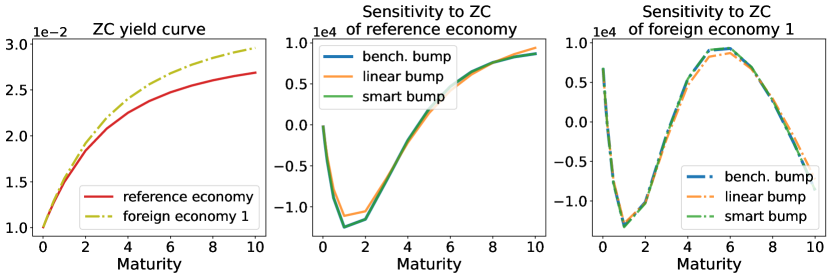
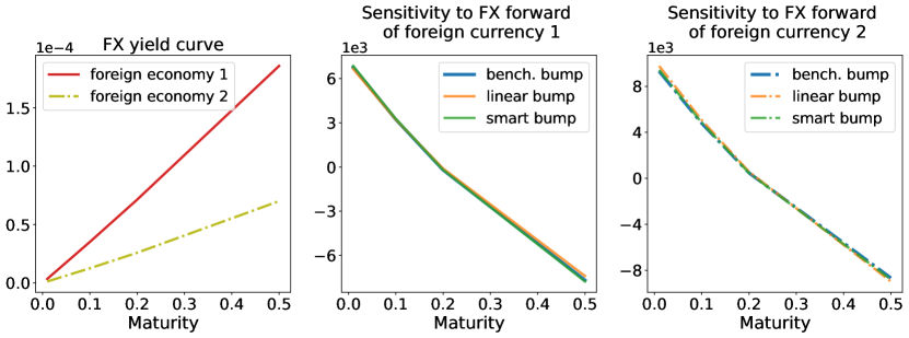
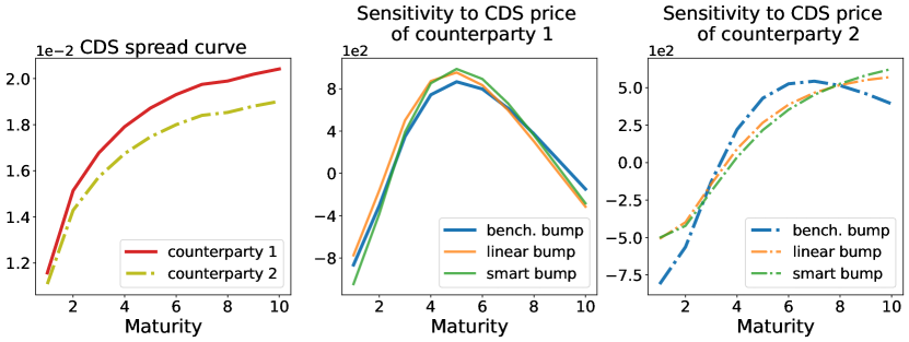
Figure 2: Sensitivities to prices of selected zero-coupons (ZCs) (top), FX forward contracts (middle), and CDS contracts (bottom), estimated by Jacobian transformations from benchmark and fast (linear and smart) bump sensitivities to the pricing model parameters. ZC and FX yield curves are constructed from ZC and FX forward prices through the transformation $\cdot\mapsto-\frac{\log(\cdot)}{T}$, where $T$ denotes the maturity.

The times taken to generate the model sensitivities of Table 2 and the corresponding market sensitivities are recorded in Table 3. The linear and smart bump calculations use the same $m$ Brownian driving paths $\omega$ of the pricing model as the one used for the Monte Carlo computation of ${\rm CVA}_{0}(\rho_{0})$. The speedups of the linear and smart bump sensitivities are almost identical, of about 90 with respect to the benchmark bump sensitivities. In Figure 3(b) page 3, the increasing curves in the left panel highlight the almost linear growth of the speedup of the linear and smart bump sensitivities with respect to the benchmark ones when the number $p$ of pricing model parameters increases, but with also increasing errors displayed in the middle panel. The smart bump sensitivities have smaller confidence interval than the linear bump sensitivities for all tested $p$. Combining with the timing result, we conclude that the smart bump sensitivities outperform the linear bump sensitivities in this CVA use case. This is confirmed by the right panel of Figure 3(b), where for all tested $p$ the complexity of linear bump sensitivities is higher than the one of smart bump sensitivities, itself very close (as expected) to the one of the benchmark bump sensitivities.

	Market sensitivities
	Parameter sensitivities			Jacobian	Total
	Simul.	Lin. regr.	Total
bench.	12m48s	N/A	12m48s(1$\times$)	30s	13m18s(1$\times$)
linear	8.6s	0.1s	8.7s(88.5$\times$)		38.7s(20.6$\times$)
smart	8.5s	N/A	8.5s(90.0$\times$)		38.5s(20.7$\times$)

Table 3: Computation times (and speedups “$\times$” in parentheses) for CVA bump sensitivities shown in Table 2. The time of the benchmark bump sensitivities contains diagonal gamma estimation (needed for the “bench. bump sensis w/ $\Gamma$” in Table 6 page 6), which amounts to an extra 5 seconds needed for computing the baseline ${\rm CVA}_{0}(\rho_{0})$ (the ${\rm CVA}_{0}(\varrho_{0})$ and ${\rm CVA}_{0}(\bar{\varrho}_{0})$ being already needed for the deltas). Here and in Figure 3(b) page 3 likewise, the times exclude the infrastructure initialization times taken once for all computations (allocating GPU memory, compiling CUDA kernel, etc.), which amount to $10$ to $30$ seconds depending on $p$.

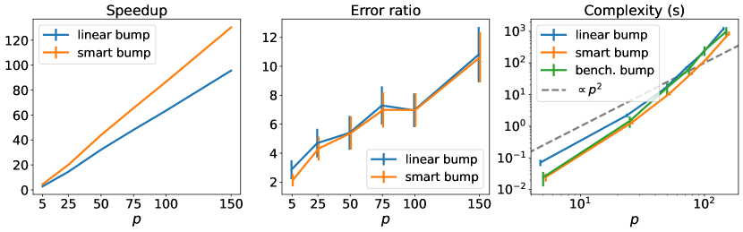
(a) Performance in Black-Scholes computations

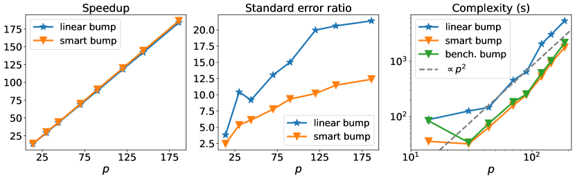
(b) Performance in CVA computations

Figure 3: Comparison of performance of linear and smart bump sensitivities as a function of the number of model parameters $p$ fixing $m=2^{16}$ in (a) and $m=2^{17}$ in (b), using benchmark bump sensitivities as references. The speedups displayed in the left panels are obtained by dividing the execution times for benchmark sensitivities by the execution times for linear or smart bump sensitivities. For each value of $p$, the errors displayed in the middle panel are: in the Black-Scholes case, the mean of the $p$ ratios between the relative error of the linear (resp. smart) bump sensitivity and the relative error of the benchmark sensitivity; in the CVA case, the median of the $p$ ratios between the Monte Carlo standard errors of the linear (resp. smart) bump sensitivity and of the benchmark sensitivity. The complexities in the right panels are defined as the projected times of reaching a relative error (for Black-Scholes) or relative standard error (for CVA) of $1\%$ given the $1/\sqrt{|\mbox{sample size}|}$ scaling of the error and standard error, with $|\mbox{sample size}|=m$ for linear and benchmark bumps and $m/p$ for smart bumps; that is, $\mbox{projected time (i.e.\ complexity)}=\mbox{exec.\ time}\times 10^{4}\mbox{ \big{(}relative (standard) error\big{)}}^{2}$. The $\sqrt{|\mbox{sample size}|}$ above is justified as explained after (5) for linear bumps and by the central limit theorem for benchmark and smart bumps. The performance metrics of the Black-Scholes computations rely on $64$ Monte Carlo simulation runs per $p$, with associated confidence intervals computed according to the principle of uncertainty propagation in (Lee and Forthofer, 2005, Chapter 4 page 22). The performances of CVA sensitivities are produced from a single Monte Carlo simulations run per $p$ (as for a given run we only have access to CVA sensitivities errors in the sense of standard errors, which cannot be aggregated across different runs).

4 Learning the Future CVA

Equivalently to the second line in (9),

$$\begin{aligned} &\mathrm{CVA}_{t}(\cdot)=\operatorname*{arg\,min}_{\Phi\in\mathcal{B}}\mathbb{E}\Big{[}\big{(}\xi_{t,T}-\Phi(X_{t},\varrho_{t})\big{)}^{2}\Big{]},\end{aligned}$$ (11)

where $\mathcal{B}$ is the set of the Borel measurable functions of $(x,\rho)$. We denote by ${{\rm CVA}}_{t}^{\theta}(X_{t},\varrho_{t})$ the conditional CVA at time $t=ih>0$ learned by a neural network with parameters $\theta$ on the basis of simulated pairs $(X_{t},\varrho_{t})$ and cash flows $\xi_{t,T}$. The conditional CVA pricing function ${{\rm CVA}}_{t}^{\theta}(x,\rho)$ is obtained by replacing $\mathbb{E}$ by a simulated sample mean $\widehat{\mathbb{E}}$ and $\mathcal{B}$ by a neural net (or linear as a special case) search space in the optimization problem (11). The latter is then addressed numerically by Adam mini-batch gradient descent on the basis of simulated pairs $(X_{t},\varrho_{t})$ as features and $\xi_{t,T}$ as labels: see Algorithm 2, in the baseline and risk modes.

input : Calibrated pricing model parameters $\rho_{0}=(y_{0},\epsilon_{0})$ (with client default indicators $X_{0}$ all equal to 0), a CVA pricing time $t=ih>0$, a number of paths $m$ with $n$ pricing time steps (and daily Euler simulation step) of the pricing model, a number of training epochs $E$ (e.g. 1000) of the (neural network or linear) learning model for ${\rm CVA}_{t}(X_{t},\varrho_{t})$, a partition $B$ of $\{1,\dots,m\}$ into mini-batches. Adam optimizer set by default.

1

output : one trained set $\theta$ of the parameters of the predictor ${\rm CVA}^{\theta}_{t}(x,y)\approx{\rm CVA}_{t}(x,y)$ in the baseline mode or ${\rm CVA}^{\theta}_{t}(x,y,\epsilon)\approx{\rm CVA}_{t}(x,y,\epsilon)$ in the risk mode.

2

3if baseline mode then

4       Set $\epsilon_{j}=\epsilon_{0}$, for $j=1\,..\,m$

5else if risk mode then

6       Draw $m$ i.i.d. bumped exogenous model parameters $\epsilon_{j}$ from the distribution $\mathcal{N}\Big{(}\epsilon_{0},\mathrm{diag}\big{(}{\sigma^{2}}\epsilon_{0}\odot\epsilon_{0}\big{)}\Big{)}$

7 end if

8For each $j\in 1\,..\,m$ with associated $\rho_{j}=(y_{0},\epsilon_{j})$ and driving Brownian path $\omega_{j}$, simulate one pricing model path $(X,Y)(\rho_{j};\omega_{j})$ starting from $(0,y_{0})$ with exogenous model parameters $\epsilon_{j}$ and compute the corresponding $\xi_{t,T}(\rho_{j};\omega_{j})$

9Initialize a neural network ${\rm CVA}^{\theta}_{t}(x,y)$ in the baseline mode or ${\rm CVA}^{\theta}_{t}(x,y,\epsilon)$ in the risk mode

10Define the loss function $\mathcal{L}(\theta,batch)=$ sample mean over trajectories in $batch\in B$ of the (cf. (11)) $\Big{(}\xi_{t,T}(\rho_{j};\omega_{j})-\Phi^{\theta}_{j}\Big{)}^{2}$, with $\Phi^{\theta}_{j}={\rm CVA}^{\theta}_{t}\Big{(}X_{t}(\rho_{j};\omega_{j}),Y_{t}(\rho_{j};\omega_{j}\Big{)}$ in the baseline mode or ${\rm CVA}^{\theta}_{t}\Big{(}X_{t}(\rho_{j};\omega_{j}),Y_{t}(\rho_{j};\omega_{j}),\epsilon_{j}\Big{)}$ in the risk mode

11 for $\text{epoch}=1,\dots,E$ do

12       for $\text{batch}\in B$ do

13             $\theta\leftarrow\text{AdamStep}(\mathcal{L}(\theta,batch))$

14            

15       end for

16      

17 end for

18

Algorithm 2 Learning CVA${}_{t}(X_{t},\varrho_{t})$ at some future time $t>0$ in the baseline or risk mode. The distribution of $\varepsilon$ in the risk mode can be set exogenously, as displayed above for simplicity, or assessed statistically on a historical basis, as done in the SIMM context of Albanese, Caenazzo, and Syrkin (2017).

4.1 Twin Monte Carlo Validation Procedure

A key asset of probabilistic machine learning procedures for any conditional expectation such as $\Pi_{0}(\varrho)$ in Section 2 is the availability of the companion “twin Monte Carlo validation procedure” of Abbas-Turki et al. (2023, Section 2.4), allowing one to assess the accuracy of a predictor. Let $\xi^{(1)}(\varrho)$ and $\xi^{(2)}(\varrho)$ denote two copies of $\xi(\varrho)$ independent given $\varrho$, i.e. such that $\mathbb{E}\big{[}f(\xi^{(1)}(\varrho))g(\xi^{(2)}(\varrho))\big{|}\varrho\big{]}=\mathbb{E}\big{[}f(\xi^{(1)}(\varrho))\big{|}\varrho\big{]}\mathbb{E}\big{[}g(\xi^{(2)}(\varrho))\big{|}\varrho\big{]}$ holds for any Borel bounded functions $f$ and $g$. The twin Monte Carlo validation procedure for a predictor $\Phi(\varrho)$ of $\Pi_{0}(\varrho)=\mathbb{E}(\xi(\varrho)|\varrho)$ consists in estimating by Monte Carlo

$$\begin{aligned} \mathbb{E}\Big{[}\Phi(\varrho)^{2}-\big{(}\xi^{(1)}(\varrho)+\xi^{(2)}(\varrho)\big{)}\Phi(\varrho)+\xi^{(1)}(\varrho)\xi^{(2)}(\varrho)\Big{]}=\mathbb{E}\Big{[}\Big{(}\Phi(\varrho)-\mathbb{E}\big{(}\xi(\varrho)\big{|}\varrho\big{)}\Big{)}^{2}\Big{]},\end{aligned}$$ (12)

as it follows from the tower rule by conditional independence: see Algorithm 3.

input : out-of-sample $\{(\rho_{j},\xi_{j}^{(1)},\xi_{j}^{(2)})\}_{j=1}^{m}$ with independent draws $\rho_{j}$ of $\varrho$ and $\xi_{j}^{(1)},\xi_{j}^{(2)}$ independent copies of $\xi$ given $\varrho=\rho_{j}$, $norm$ (set to $1$ by default)

1

output : Estimation of the normalized root mean square relative error and its $95\%$-confidence upper bound for a predictor $\Phi(\varrho)$ of $\Pi_{0}(\varrho)=\mathbb{E}(\xi|\varrho)$

2Compute $twin\mbox{-}stat=\frac{1}{m}\sum_{j=1}^{m}\left[(\Phi(\rho_{j}))^{2}-(\xi^{(1)}_{j}+\xi^{(2)}_{j})\Phi(\rho_{j})+\xi^{(1)}_{j}\xi^{(2)}_{j}\right]$

3Compute $twin\mbox{-}stdev=\sqrt{\frac{1}{m}\sum_{j=1}^{m}\left[(\Phi(\rho_{j}))^{2}-(\xi^{(1)}_{j}+\xi^{(2)}_{j})\Phi(\rho_{j})+\xi^{(1)}_{j}\xi^{(2)}_{j}-twin\mbox{-}stat\right]^{2}}$

4Compute $twin\mbox{-}up=\sqrt{twin\mbox{-}stat+\frac{2}{\sqrt{m}}twin\mbox{-}stdev}$

5if $twin\mbox{-}stat>0$ then

6      

7      Compute $twin\mbox{-}err=\sqrt{twin\mbox{-}stat}/norm$

8else

9      

10      Set $twin\mbox{-}err$ to N/A

11 end if

12Output $twin\mbox{-}err$ and $twin\mbox{-}ub:=twin\mbox{-}up/norm$

Algorithm 3 Twin Monte Carlo validation for a predictor $\Phi(\varrho)$ of $\Pi_{0}(\varrho)=\mathbb{E}(\xi|\varrho)$.

The estimate $twin\mbox{-}stat$ of the square error can be negative in this algorithm. Thus, the $95\%$ upper bound of square error, remaining positive most of the times, is calculated alongside the square error itself. We emphasize that the ensuing twin errors measure the performance of the predictor, but not of the associated sensitivities, as a low error of the predictor induces no constraint on the error for the derivatives.

$t$ (in yr)	Baseline mode			Risk mode
	Nested MC	NN	Linear	Nested MC	NN	Linear
$0.01$	N/A(4.3%)	N/A(4.3%)	N/A(4.5%)	N/A(4.3%)	2.1%(5.0%)	3.0%(5.5%)
$0.1$	6.6%(8.0%)	5.7%(7.3%)	6.8%(8.2%)	6.6%(8.0%)	9.8%(10.8%)	9.8%(10.8%)
1	9.2%(10.3%)	9.7%(10.8%)	10.4%(11.4%)	9.4%(10.5%)	22.1%(22.6%)	22.3%(22.9%)
$3.5$	8.8%(10.1%)	12.0%(13.5%)	15.7%(17.3%)	9.7%(11.5%)	26.0%(27.0%)	27.0%(28.2%)

Table 4: The mean and ($95\%$ upper bound) for the relative twin error normalized by ${\rm CVA}_{0}(\rho_{0})$ (cf. Algorithm 3) of nested Monte Carlo ${\rm CVA}_{t}$, neural network ${\rm CVA}_{t}$, and linear regression ${\rm CVA}_{t}$, for $t=0.01,0.1,1$, and $3.5\approx T/3$ years (where the CVA of a portfolio of swaps is deemed the most volatile), in the baseline and risk modes.

Table 4 shows the twin scores of neural network and linear regression versus nested Monte Carlo predictors of CVA${}_{t}(X_{t},\varrho_{t})$ in the baseline and risk modes. In both modes, all three methods have comparable performance for small $t$ ($0.01$ and $0.1$ years). The linear learning model for ${\rm CVA}^{\theta}_{t}(x,\rho)$ does not require sophisticated training like the neural network but only linear algebra, it converges equally well for $t=0.01$ and $0.1$, but falls short at one year, where the nonlinearity of CVA${}_{t}(x,\rho)$ becomes significant: for $t=1$ and $3.5$ years, the neural network outperforms the linear regression significantly. As illustrated by the left panel of Figure 1 in (Abbas-Turki et al., 2023, Section 2), this nonlinearity and the necessity of neural network would become more stringent with option portfolios, possibly for lower $t$ already. In the baseline mode, the learned ${\rm CVA}_{t}(X_{t},\varrho_{t})$ can occasionally be more accurate than its nested Monte Carlo counterpart, which is also much slower: for a given $t$, the nested Monte Carlo CVA (with $m=2^{17}$ outer paths and 1024 inner paths throughout the paper) takes approximately 40 minutes, while simulating the data and training a neural net CVA with 2 hidden layers and softplus activation (resp. regressing a linear CVA) takes roughly 30 (resp. 25) seconds. In the risk mode, the neural network is less accurate than nested Monte Carlo: the input dimension of the neural network becomes 35 for $(x,y)$ plus 63 for $\epsilon$ in the risk mode versus 35 simply in the baseline mode, hence training ${\rm CVA}^{\theta}_{t}(x,\rho)$ becomes harder (or would require more data) and the resulting predictor becomes less accurate than nested Monte Carlo. For $t=3.5$ the neural network prediction is bad, but not as bad as the linear prediction. A better neural network predictor might be achievable by fine-tuning the SGD or enriching the simulated dataset and/or the architecture of the network. Since we only need the risk mode for $t\leq 1$ in the dowstream tasks of Sections 5-6, we did not venture in these directions.

5 Run-off CVA Risk

An economic (or “internal”) view gained from simulating the movements of model or/and market risk factors and obtaining risk measures of CVA fluctuations is an important dimension of the CVA capital regulatory requirements of a bank, in the context of its supervisory review and evaluation process (SREP): quoting https://www.bankingsupervision.europa.eu/legalframework/publiccons/html/icaap_ilaap_faq.en.html (last accessed June 6 2024), “the risks the institution has identified and quantified will play an enhanced role in, for example, the determination of additional own funds requirements on a risk-by-risk basis.”

The focus of this section is on

$$\begin{aligned} \delta{\rm CVA}^{\theta}_{t}+{\rm LGD}_{t},\;\mbox{where }\delta{\rm CVA}^{\theta}_{t}={\rm CVA}^{\theta}_{t}(X_{t},\varrho_{t})-{\rm CVA}_{0}(\rho_{0})\end{aligned}$$ (13)

(cf.  (8)-(9)), assessed in the risk mode, where $\varrho_{t}=(Y_{t}(y_{0},\varepsilon),\varepsilon)$ and $\varepsilon$ follows $\mathcal{N}\Big{(}\epsilon_{0},\mathrm{diag}\left(t(1\%)^{2}\epsilon_{0}\odot\epsilon_{0}\right)\Big{)}$. The random variable ($\delta{\rm CVA}^{\theta}_{t}+{\rm LGD}_{t}$) reflects a dynamic but also run-off view on CVA and counterparty default risk altogether, as opposed to the stationary run-on CVA risk view of Section 6. We assess CVA risk, counterparty default risk, and both risks combined, on the basis of value-at-risks (VaR) and expected shortfalls (ES) of $\delta{\rm CVA}^{\theta}_{t}$ and LGD_t in the risk mode, reported for $t=0.01,0.1,1$ yr and various quantile levels $\alpha=95,97.5$ or $99\%$ in Table 5. The middle-point of $97.5\%$ for the ES fits a nowadays reference $99.9\%$ value-at-risk reference level, via the conventional mapping between a $97.5\%$ ES and a $99\%$ VaR in a Gaussian setup, also considering that our baseline parametrization reflects market conditions at a 90% level of stress (cf. the high CDS spreads visible in the bottom left panel of Figure 2). The results of Table 5 page 5 emphasize that CVA and counterparty default risks assessed on a run-off basis are primarily driven by client defaults, especially at higher quantile levels. As visible in the right plots, for $t=0.01$ and $0.1$, there are few client defaults and the right tail of the distribution of $\delta{\rm CVA}^{\theta}_{t}+{\rm LGD}_{t}$ is dominated by the term $\delta{\rm CVA}^{\theta}_{t}$. For $t=1$, instead, the ${\rm LGD}_{t}$ term takes the lead, significantly shifting the right tail of the distribution upward.

$t=0.01$	$\delta{\rm CVA}^{\theta}_{t}$	${\rm LGD}_{t}$	$\delta{\rm CVA}^{\theta}_{t}$ $+{\rm LGD}_{t}$
Expectation	-9	0.28	-8
VaR 95%	268	0	268
VaR 97.5%	323	0	323
VaR 99%	388	0	389
ES 95%	344	0.28	345
ES 97.5%	395	0.28	397
ES 99%	460	0.28	464

$t=0.1$	$\delta{\rm CVA}^{\theta}_{t}$	${\rm LGD}_{t}$	$\delta{\rm CVA}^{\theta}_{t}$ $+{\rm LGD}_{t}$
Expectation	56	7	63
VaR 95%	939	0	953
VaR 97.5%	1,124	0	1,145
VaR 99%	1,347	0	1,389
ES 95%	1,192	7	1,243
ES 97.5%	1,361	7	1,445
ES 99%	1,571	7	1,740

$t=1$	$\delta{\rm CVA}^{\theta}_{t}$	${\rm LGD}_{t}$	$\delta{\rm CVA}^{\theta}_{t}$ $+{\rm LGD}_{t}$
Expectation	75	502	578
VaR 95%	2,942	3,621	4,597
VaR 97.5%	3,746	7,309	7,190
VaR 99%	4,796	11,997	11,757
ES 95%	4,122	8,846	8,980
ES 97.5%	4,953	12,383	12,297
ES 99%	6,102	17,004	17,048

Table 5: $\delta{\rm CVA}^{\theta}_{t},$ LGD_t and their sum (${\rm CVA}_{0}(\rho_{0})=5,027$). (Left) Risk measures. (Right) qq plots against $\delta{\rm CVA}^{\theta}_{t}$ used as a benchmark (corresponding to the diagonal). The red circles correspond to the VaRs 95%, 97.5% and 99%.

5.1 Run-off CVA Hedging

Let (in vector form) CF represent the cumulative cash flows process of the market instruments of Section 3.1, with price process $Z_{t}=\mathbb{E}(\textrm{CF}_{T}-\textrm{CF}_{t}|X_{t},\varrho_{t}),t\in 0\,..\,nh=T$, and let

$$\begin{aligned} \delta Z_{t}=Z_{t}(X_{t},\varrho_{t})-z_{0}\end{aligned}$$ (14)

denote the difference between the market prices $Z_{t}(X_{t},\varrho_{t})$ and their time-0 baseline price $z_{0}$. By loss $L^{\theta}_{t}$, we mean the following hedged loss(-and-profit) of the CVA desk over the risk horizon $t$:

$$\begin{aligned} L^{\theta}_{t}=\delta{\rm CVA}^{\theta}_{t}+{\rm LGD}_{t}-(\delta Z_{t}+\textrm{CF}_{t})^{\top}\Delta-c,\end{aligned}$$ (15)

where the hedging ratio $\Delta\in\mathbb{R}^{q}$ is treated as a free parameter, while $c$ is deduced from $\Delta$ through the constraint that ${\mathbb{E}}L^{\theta}_{t}=0$ (or $\widehat{\mathbb{E}}L^{\theta}_{t}=0$ in our numerics). The constant $c$, which is equal to 0 (modulo the numerical noise) in the baseline mode where ${\rm CVA}+{\rm LGD}$ and $Z+\textrm{CF}$ are both martingales, can be interpreted in terms of a hedging valuation adjustment (HVA) in the spirit of Albanese, Benezet, and Crépey (2023), i.e. a provision for model risk. Albanese et al. (2023) develop how, such a provision having been set apart in a first stage, the loss $L^{\theta}_{t}$, thus centered via the “HVA trend” $c$ (i.e. $c=-\mathbb{E}\delta{\rm HVA}_{t}={\rm HVA}_{0}-\mathbb{E}{\rm HVA}_{t}$), deserves an economic capital, which we quantify below as an expected shortfall of $L^{\theta}_{t}$.

Bump sensitivities $\Delta=\Delta^{bump}$ can be used in (15) but they are expected to be inappropriate for dealing with client defaults. As an alternative approach yielding hedging ratios, HVA trend and economic capital at the same time, one can use

$$\Delta^{ec}=\operatorname*{arg\,min}\limits_{\Delta\in\mathbb{R}^{q}}\mathbb{ES}\left(L^{\theta}_{t}\right).$$ (16)

Following Rockafellar and Uryasev (2000), (16) can be reformulated as the following convex optimization problem:

$$\left(\Delta^{ec},k^{ec}\right)=\operatorname*{arg\,min}\limits_{\Delta\in\mathbb{R}^{q},k\in\mathbb{R}}k+(1-\alpha)^{-1}\mathbb{E}\left[\left(L^{\theta}_{t}-k\right)^{+}\right],$$ (17)

where $k^{ec}$ is then the value-at-risk (quantile of level $\alpha$) of the corresponding $L^{\theta}_{t}$. Note that one could also easily account for transaction costs in this setup, which is nothing but a deep hedging approach over one time step for computing the HVA trend $c$ and the hedging policy $\Delta^{ec}$ compressing the ensuing economic capital and its cost. Note that the constraint $\mathbb{E}L^{\theta}_{t}=0$, motivated financially after (15), is also necessary numerically to stabilize the training of the EC sensitivities.

As a possible (simpler) variation on the economic capital (EC) run-off sensitivities (16)-(17), we also consider the following PnL explain (PLE) run-off sensitivities:

$$\Delta^{ple}=\operatorname*{arg\,min}\limits_{\Delta\in\mathbb{R}^{q}}\mathbb{E}[(L^{\theta}_{t})^{2}].$$ (18)

Once ${\rm CVA}^{\theta}_{t}(X_{t},\varrho_{t})$ learned from the cash flows $\xi_{t,T}(\varrho_{t})$ the way described in Algorithm 2 / risk mode, the EC sensitivities (16) are computed by stochastic gradient descent based on an empirical version of (17); the PLE sensitivities are computed by performing a linear regression corresponding to an empirical version of (18): cf. lines 9–13 of Algorithm 4 page 4 (which corresponds to the CVA run-on setup of Section 6).

By unexplained PnL UPL (resp. economic capital EC), we mean the standard error (resp. expected shortfall) of $L^{\theta}_{t}$. As performance metrics, we consider a backtesting, out-of-sample UPL (resp. EC with $\alpha=95\%$) for $\Delta=0$, divided by UPL (resp. EC with $\alpha=95\%$) for each considered set of sensitivities: the higher the corresponding “compression ratios”, the better the corresponding sensitivities. For each simulation run below (here and in Section 6), we use $m=2^{17}$ paths to estimate the PLE and EC sensitivities and we generate other $m=2^{17}$ paths for our backtest.

The left panels in Figure 4 compare the hedging performance of benchmark bump versus EC or PLE sensitivities for $t=0.01,0.1,$ and $1$ yr. The unhedged case corresponds to the red horizontal dash-dot lines. Consistent with their definitions, the PLE sensitivities always (even though we are out-of-sample) yield the highest unexplained PnL compression ratios, while the EC sensitivities, except for $t=0.01$, yield the highest EC compression ratio. As expected, bump sensitivities provide very poor hedging performance (we omitted fast bump sensitivities, which provide results similar to the benchmark ones). At the risk horizon $t=0.01$, client defaults are rare (only occurring on $0.017\%$ of the scenarios) and a bump sensitivities hedge reduces risk, but much less so than the EC or PLE sensitivities hedges. For $t=0.1$ and 1 yr, hedging by bump sensitivities is even counterproductive, worsening both unexplained PnL and economic capital compared to the unhedged case; EC and PLE sensitivities hedges achieve significant unexplained PnL and economic capital compression, but this comes along with very high HVA trends $c$.

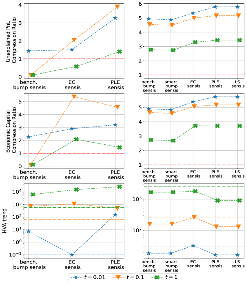
Figure 4: Compression ratios of UPL (top), EC (middle), and HVA trends $c$ (bottom), for various $\delta{\rm CVA}^{\theta}_{t}+{\rm LGD}_{t}$ hedging approaches in Section 5.1 (left), and $\delta{\rm CVA}^{\theta}_{(t)}$ hedging approaches in Section 6.1 (right). Horizontal dash-dot lines correspond to the unhedged case with $\Delta=0$ in (15) and (20).

The expected conclusion of this part is that for properly hedging CVA in the run-off mode, one should first replicate the impact of the defaults with appropriate CDS positions (or decide to warehouse default risk, especially if CDSs are not liquidly available), rather than trying to hedge “on average”, which only makes sense for CVA assessed in the run-on mode. The latter corresponds to the right panels in Figure 4, to be commented upon in Section 6.1.

6 Run-on CVA Risk

With $\cdot_{(t)}$ in $\varepsilon_{(t)}$ referring to the dependence of the variance $\sigma^{2}$ of $\varepsilon-\epsilon_{0}$ (in the notation of Algorithm 2) in $t$ in what follows, namely $\mathbb{V}\mathrm{ar}(\varepsilon_{(t)})=t\times 0.01\%$, denoting by $Y_{t}(y_{0},\varepsilon_{(t)})$ the $Y$ process at time $t$ starting from $y_{0}$ at 0 and for model parameters set to $\varepsilon_{(t)}$, and by $\varrho_{(t)}=\big{(}Y_{t}(y_{0},\varepsilon_{(t)}),\varepsilon_{(t)}\big{)}$, let (cf. (14))

$$\begin{aligned} &\delta\varrho_{(t)}=(Y_{t}(y_{0},\varepsilon_{(t)})-y_{0},\varepsilon_{(t)}-\epsilon_{0})=\varrho_{(t)}-\rho_{0},\;\delta Z_{(t)}=Z_{0}(\varrho_{(t)})-z_{0},\\ &\delta{\rm CVA}_{(t)}={\rm CVA}_{0}(\varrho_{(t)})-{\rm CVA}_{0}(\rho_{0}).\end{aligned}$$ (19)

The fact that we consider the time-0 ${\rm CVA}_{0}(\varrho_{(t)})$ (see after (9)) and likewise $Z_{0}(\varrho_{(t)})$ here, as opposed to ${\rm CVA}_{t}(X_{t},\varrho_{t})$ and $Z_{t}(X_{t},\varrho_{t})$ in Section 5, is in line with an assessment of risk on a run-on portfolio and customers basis and with a siloing of CVA vs. counterparty default risk, which have both become standard in regulation and market practice. Various predictors of $\delta{\rm CVA}_{(t)}$ can be learned directly from the simulated model parameters $\varrho_{(t)}$ and cash flows $\xi_{0,T}(\varrho_{(t)})-\xi_{0,T}(\rho_{0})$ (as opposed to and better than learning $\delta{\rm CVA}_{(t)}$ via ${\rm CVA}_{0}(\varrho_{(t)})$, which would involve more variance): nested Monte Carlo estimator, neural net regressor $\delta{\rm CVA}^{\theta}_{(t)}$, linear(-diagonal quadratic) regressors against $\delta\varrho_{(t)}$ or $\delta Z_{(t)}$ referred to as LS (for “least squares”) below. The neural network used for training $\delta{\rm CVA}^{\theta}_{(t)}$ based on simulated data $(\varrho_{(t)}-\rho_{0},\xi_{0,T}(\varrho_{(t)};\omega)-\xi_{0,T}(\rho_{0};\omega))$ as per line 8 of Algorithm 4 has one hidden layer with two hundred hidden units and softplus activation functions.

Table 6 displays some twin upper bounds and risk measures of $\delta{\rm CVA}_{(t)}$ computed with these different approximations, as well as with linear(- diagonal quadratic) Taylor expansions in $\delta\varrho_{(t)}$ or $\delta Z_{(t)}$ with coefficients estimated as benchmark or smart bump sensitivities.

In terms of the twin upper bounds, the nested CVA has the best accuracy, but (for a given risk horizon $t$) it takes about 2 hours, versus about one minute of simulation time for generating the labels, plus 30 seconds for training by neural networks and 2-3 seconds for LS regression. The neural network excels at large $t$, where the non-linearity becomes significant, while being outperformed by the linear methods at small $t$, where $\delta{\rm CVA}_{(t)}$ is approximately linear. With diagonal gamma ($\Gamma$) elements taken into account, the performance of the LS regressor improves at large $t$. The linear quadratic Taylor expansions show relatively good twin upper bounds for small $t$, but worsen for large $t$.

Regarding now the risk measures, the nested $\delta{\rm CVA}_{(t)}$ and the neural network $\delta{\rm CVA}^{\theta}_{(t)}$ provide more conservative VaR and ES estimates than any linear(-quadratic) proxy in all cases. Surprisingly, even though ${\rm CVA}_{0}(\varrho_{(t)})$ in $\delta{\rm CVA}_{(t)}$ is a function of $\varrho_{(t)}$, for $t=1$ the linear(-quadratic) proxies in $\delta Z_{(t)}$ outperform those in $\varrho_{(t)}$, in terms both of twin error and of consistency of the ensuing risk measures with those provided by the nonparametric (neural net and nested) references. Also note that, when compared with the nonparametric approaches again, the smart bump sensitivities proxy in $\delta Z_{(t)}$ yields results almost as good as the much slower benchmark bump sensitivities proxy in $\delta Z_{(t)}$ (see Tables 3 and 7 pages 3 and 7).

$t$	risk measure	nonparametric		linear quadratic in $\delta\varrho_{(t)}$			linear quadratic in $\delta Z_{(t)}$
		nested $\delta{\rm CVA}_{(t)}$	$\delta{\rm CVA}^{\theta}_{(t)}$	bench. bump sensis w/ $\Gamma$	smart bump sensis	LS sensis w/ $\Gamma$	bench. bump sensis	smart bump sensis	LS sensis w/ $\Gamma$
0.01	twin-ub	11	29	13	15	18	23	23	18
	VaR 95%	364	315	312	306	302	315	312	308
	VaR 97.5%	431	369	366	358	354	370	367	362
	VaR 99%	510	431	429	418	415	435	431	424
	ES 95%	454	387	384	375	372	389	385	380
	ES 97.5%	514	434	432	421	417	437	433	427
	ES 99%	585	491	489	476	473	495	490	484
0.1	twin-ub	59	103	110	111	109	101	104	94
	VaR 95%	1,223	1,189	1,154	1,101	1,148	1,147	1,138	1,151
	VaR 97.5%	1,431	1,383	1,340	1,266	1,327	1,330	1,318	1,332
	VaR 99%	1,686	1,618	1,562	1,463	1,539	1,554	1,542	1,556
	ES 95%	1,504	1,449	1,403	1,321	1,386	1,396	1,383	1,396
	ES 97.5%	1,693	1,622	1,570	1,467	1,544	1,559	1,545	1,561
	ES 99%	1,923	1,830	1,769	1,638	1,731	1,757	1,740	1,757
1	twin-ub	325	693	1,244	1,307	1,113	932	943	743
	VaR 95%	7,097	6,992	6,365	5,300	6,440	5,867	5,831	6,676
	VaR 97.5%	8,433	8,199	7,451	5,897	7,432	6,737	6,686	7,838
	VaR 99%	10,333	9,887	8,991	6,646	8,812	7,914	7,846	9,493
	ES 95%	9,163	8,805	8,077	6,142	7,956	7,162	7,097	8,492
	ES 97.5%	10,654	10,090	9,309	6,715	9,032	8,075	7,988	9,792
	ES 99%	12,781	11,869	11,161	7,456	10,598	9,339	9,216	11,677

Table 6: Risk measures of $\delta{\rm CVA}_{(t)}$ computed by Monte Carlo using $\delta{\rm CVA}_{(t)}$ simulated by various predictors. The three lowest (i.e. best) twin errors (without normalization, cf. Algorithm 3 page 3) and the three highest (i.e. most conservative) risk estimates on each row are emphasized in bold.

6.1 Run-on CVA Hedging

Let

$$\begin{aligned} &L^{\theta}_{(t)}=\delta{\rm CVA}_{(t)}^{\theta}-(\delta Z_{(t)})^{\top}\Delta-c\end{aligned}$$ (20)

(cf. (14) and (19)). As in Section 5, the “HVA trend” $c$ (here “$=-\mathbb{E}\delta{\rm HVA}_{(t)}={\rm HVA}_{0}-\mathbb{E}{\rm HVA}_{(t)}$”) is deduced from $\Delta$ through the constraint that ${\mathbb{E}}L^{\theta}_{(t)}=0$ (or $\widehat{\mathbb{E}}L^{\theta}_{(t)}=0$ in the numerics). By EC and PLE run-on sensitivities, we mean

$$\Delta^{ec}=\operatorname*{arg\,min}\limits_{\Delta\in\mathbb{R}^{q}}\mathbb{ES}\left(L^{\theta}_{(t)}\right)\mbox{ and }\Delta^{ple}=\operatorname*{arg\,min}\limits_{\Delta\in\mathbb{R}^{q}}\mathbb{E}[(L^{\theta}_{(t)})^{2}],$$ (21)

where $\mathbb{ES}$ means 95% expected shortfall as in Section 5.1. Once $\delta{\rm CVA}^{\theta}_{(t)}$ learned from simulated $\varrho_{(t)}$ and $\xi_{0,T}(\varrho_{(t)})-\xi_{0,T}(\rho_{0})$ the way mentioned after (19), these sensitivities are computed much like their run-off counterparts of Section 5. Even simpler (but still optimized) LS (run-on) sensitivities are obtained without prior learning of $\delta{\rm CVA}_{(t)}$, just by regressing linearly $\xi_{0,T}(\varrho_{(t)})-\xi_{0,T}(\rho_{0})$ against $\delta Z_{(t)}$ the way explained after (19) (purely linear LS regression here as opposed to linear diagonal quadratic LS regression in Table 6, due to our hedging focus of this part). These LS sensitivities are thus obtained much like the linear bump sensitivities of Algorithm 1, except for the scaling of the bumps that are used in the corresponding $\varrho_{(t)}$, and the fact that these LS sensitivities are computed directly in the market variables, without Jacobian transformation. The derivation of the LS, EC, and PLE run-on sensitivities is summarized in Algorithm 4. Their computation times are reported in Table 7. The right panels in Figure 4 page 4 show the run-on CVA hedging performance of different candidate sensitivities. All the risk compression ratios decrease with the risk horizon $t$. All sensitivities reduce both the unexplained PnL and economic capital by at least 2.5 times for $t=0.01$ and 4.5 times for $t=0.1$ and 1. Since client defaults are skipped in the run-on mode, the efficiency of bump sensitivities hedges is understandable. For each risk horizon and performance metric, the optimized sensitivities always have better results than (benchmark or smart) bump sensitivities. Among those, the PLE and LS sensitivities hedges display the highest risk compression ratios and the lowest HVA trend $c$. Unlike what we observed in the run-off mode, most sensitivities (except for EC sensitivities when $t=0.01$ or $0.1$) also compress the HVA trend $c$ compared to the unhedged case.

input : A set of calibrated initial values and model parameters $\rho_{0}=(y_{0},\epsilon_{0})$ (client default indicators $X_{0}$ all set to 0), a time horizon $t$, a number of exposure paths $m$ with $n$ pricing time steps.

1

output : Estimated sensitivities ${\Delta}$.

2 Simulate $m$ cash flows $\xi_{0,T}(\rho_{0};\omega_{j})$ as per line 6 of Algorithm 2 in the baseline mode

3Simulate $m$ realizations $\epsilon_{j}$ of $\varepsilon_{(t)}$ as per line 2 of Algorithm 2 with $\sigma=1\%\sqrt{t}$ and $y_{j}=Y^{j}_{t}(y_{0},\epsilon_{j};\tilde{\omega}_{j})$ as per line 6 of Algorithm 2, for Brownian drivers $\tilde{\omega}_{j}$ drawn independently from the $\omega_{j}$, and set $\rho_{j}=(y_{j},\epsilon_{j})$

4Simulate $m$ realizations $\xi_{0,T}(\rho_{j};\omega_{j})$ as per line 6 of Algorithm 2 in the risk mode (with common random numbers, meaning here the same $\omega_{j}$ as in line 1)

5For each $\rho_{j}$, $j=0\,..\,m$, compute the corresponding market hedging instrument prices scenario $z_{j}$

6if LS then

7       Regress linearly the $\xi_{0,T}(\rho_{j};\omega_{j})-\xi_{0,T}(\rho_{0};\omega_{j})$ against the $z_{j}-z_{0}$ by SVD. The obtained coefficients are the LS sensitivities.

8else

9       Train a neural network $\delta{\rm CVA}^{\theta}_{(t)}(y,\epsilon)$ to regress the $\xi_{0,T}(\rho_{j};\omega_{j})-\xi_{0,T}(\rho_{0};\omega_{j})$ against the $\rho_{j}-\rho_{0}.$

10      if EC then

11             Solve the left-hand side in (21) by Adam stochastic gradient descent.

12      else if PLE then

13             Solve the right-hand side in (21) by SVD linear regression.

14       end if

15      

16 end if

17

Algorithm 4 LS, EC and PLE run-on sensitivities.

[Smart] bump sensitivities		Regression sensitivities					Speedup
Model sensis	Jacobian transform	MtM simulation	LS	$\delta{\rm CVA}_{(t)}^{\theta}$ learning	PnL regression
					EC	PLE	LS	EC	PLE
12min48s [8.5s]	30s	27s	1s	6s	31s	1s	28.5 [1.4]	12.5 [0.6]	23.5 [1.1]

Table 7: Computation times for learning $\delta{\rm CVA}_{(t)}^{\theta}$ and the related sensitivities. The speedups measure the ratios of the total time taken by the benchmark bump sensitivities approach to the total time taken by each of the sensitivities.

7 Conclusion

Table 8 synthesizes our findings regarding CVA (or more general, regarding columns 1 to 3) sensitivities, as far as their approximation quality to corresponding partial derivatives (for bump sensitivities) and their hedging abilities (regarding also the optimized sensitivities) are concerned. The winner that emerges as the best trade-off for each downstream task in blue green red in the first row is identified by the same color in the list of sensitivities. bench. bump plays the role of market standard. Sensitivities that are novelties of this work are emphasized in yellow (smart bump sensitivities essentially mean standard bump sensitivities with less paths, but with the important implementation caveat mentioned at the end of Section 2.1; PLE sensitivities were already introduced in the different context of SIMM computations in Albanese et al. (2017); EC sensitivities were introduced in Rockafellar and Uryasev (2000) and are also considered in Buehler (2019)).

	sensitivities	speed	stability	local accuracy	CVA run-off hedge	CVA run-on hedge
	bench. bump	very slow	very stable	benchmark	bad	good
fast bump sensis	naive AAD bump	fast	fragile	bad	bad	bad
	yellowAAD bump	fast	fragile	average	bad	bad
	yellowlinear bump	fast	average	good	bad	good
	smart bump	fast	stable	good	bad	good
optimized sensis	EC sensis	fast	average	not applicable	good	very good
	PLE sensis	very fast	stable	not applicable	good	excellent
	yellow LS w/o $\boldsymbol{\Gamma}$	very fast	stable	not applicable	not applicable	excellent

Table 8: Conclusions regarding sensitivities and hedging. By local accuracy of a bump sensitivity, we mean the accuracy of the approximation it provides for the corresponding partial derivative. Italics means tested but not reported in tables or figures in the paper.

Regarding the assessment of CVA risk, in the run-on CVA case (see Table 9 using the same color code as Table 8), we found out that neural net regression of conditional CVA results in likely more reliable (judging by the twin scores of the associated CVA learners) and also faster value-at-risk and expected shortfall estimates than CVA Taylor expansions based on bump sensitivities (such as the ones that inspire certain regulatory CVA capital charge formulas). But an LS proxy, linear diagonal quadratic in market bumps, provides an even quicker (as it is regressed without training) and almost equally reliable view on CVA risk as the neural net CVA. In the run-off CVA case (not represented in the table), the neural net learner of CVA_t in the risk mode (or nested CVA learner alike but in much longer time) allows one to get a consistent and dynamic view on CVA and counterparty default risk altogether.

	$\delta{\rm CVA}_{(t)}$ learners	speed	stability	twin accuracy	$\delta{\rm CVA}_{(t)}$ VaR and ES
nonparametric	yellownested MC	very slow	stable	very good	very conservative
	yellowneural net	fast	average	good	conservative
linear(-quadratic) in market bumps	bench. bump	very slow	very stable	good/average for small/large $t$	aggressive
	yellow LS w/ $\boldsymbol{\Gamma}$ in $\boldsymbol{\delta Z_{t}}$	very fast	stable	good	conservative

Table 9: Conclusions regarding run-on CVA risk.

References

- Abbas-Turki et al. (2024) Abbas-Turki, L., S. Crépey, B. Li, and B. Saadeddine (2024). An explicit scheme for pathwise XVA computations. arXiv:2401.13314.
- Abbas-Turki et al. (2023) Abbas-Turki, L., S. Crépey, and B. Saadeddine (2023). Pathwise CVA regressions with oversimulated defaults. Mathematical Finance 33(2), 274–307.
- Albanese et al. (2023) Albanese, C., C. Benezet, and S. Crépey (2023). Hedging valuation adjustment and model risk. arXiv:2205.11834v2.
- Albanese et al. (2017) Albanese, C., S. Caenazzo, and M. Syrkin (2017). Optimising VAR and terminating Arnie-VAR. Risk Magazine, October.
- Albanese et al. (2021) Albanese, C., S. Crépey, R. Hoskinson, and B. Saadeddine (2021). XVA analysis from the balance sheet. Quantitative Finance 21(1), 99–123.
- Antonov et al. (2018) Antonov, A., S. Issakov, and A. McClelland (2018). Efficient SIMM-MVA calculations for callable exotics. Risk Magazine, August.
- Buehler (2019) Buehler, H. (2019). Statistical hedging. ssrn.2913250.
- Capriotti et al. (2017) Capriotti, L., Y. Jiang, and A. Macrina (2017). AAD and least-square Monte Carlo: Fast Bermudan-style options and XVA Greeks. Algorithmic Finance 6(1-2), 35–49.
- Crépey (2013) Crépey, S. (2013). Financial Modeling: A Backward Stochastic Differential Equations Perspective. Springer Finance Textbooks.
- Henrard (2011) Henrard, M. (2011). Adjoint algorithmic differentiation: Calibration and implicit function theorem. OpenGamma Quantitative Research (1). ssrn:1896329.
- Lee and Forthofer (2005) Lee, E. S. and R. N. Forthofer (2005). Analyzing complex survey data. Sage Publications.
- Matloff (2017) Matloff, N. (2017). Statistical regression and classification: from linear models to machine learning. Chapman and Hall/CRC.
- Rockafellar and Uryasev (2000) Rockafellar, R. T. and S. Uryasev (2000). Optimization of conditional value-at-risk. Journal of risk 2, 21–42.
- Saadeddine (2022) Saadeddine, B. (2022). Learning From Simulated Data in Finance: XVAs, Risk Measures and Calibration. Ph. D. thesis, Université Paris-Saclay. https://theses.hal.science/tel-03894764v1/document.
- Savine (2018) Savine, A. (2018). From model to market risks: The implicit function theorem (IFT) demystified. ssrn:3262571.