PP-TIL: Personalized Planning for Autonomous Driving with Instance-based Transfer Imitation Learning

Abstract

Personalized motion planning holds significant importance within urban automated driving, catering to the unique requirements of individual users. Nevertheless, prior endeavors have frequently encountered difficulties in simultaneously addressing two crucial aspects: personalized planning within intricate urban settings and enhancing planning performance through data utilization. The challenge arises from the expensive and limited nature of user data, coupled with the scene state space tending towards infinity. These factors contribute to overfitting and poor generalization problems during model training. Henceforth, we propose an instance-based transfer imitation learning approach. This method facilitates knowledge transfer from extensive expert domain data to the user domain, presenting a fundamental resolution to these issues. We initially train a pre-trained model using large-scale expert data. Subsequently, during the fine-tuning phase, we feed the batch data, which comprises expert and user data. Employing the inverse reinforcement learning technique, we extract the style feature distribution from user demonstrations, constructing the regularization term for the approximation of user style. In our experiments, we conducted extensive evaluations of the proposed method. Compared to the baseline methods, our approach mitigates the overfitting issue caused by sparse user data. Furthermore, we discovered that integrating the driving model with a differentiable nonlinear optimizer as a safety protection layer for end-to-end personalized fine-tuning results in superior planning performance. The code will be available at https://github.com/LinFunster/PP-TIL.

I Introduction

Autonomous driving has been a focal point of research and development over the past decade. The motion planning module stands out as a critical component within the urban autonomous driving system [1, 2]. This module typically considers factors such as safety, travel efficiency, and comfort. In practical terms, individual perceptions of comfort can vary significantly among users. For instance, some may prefer high-acceleration sports driving, while others may lean towards a more relaxed style. Offering personalized motion planning holds immense significance in enhancing user acceptance of autonomous driving. However, manually adjusting the parameters of the planning model to achieve a specified style can be challenging due to the potential for antagonistic effects of a large number of parameters. Fortunately, the data-driven approaches can effectively address this issue [3, 4].

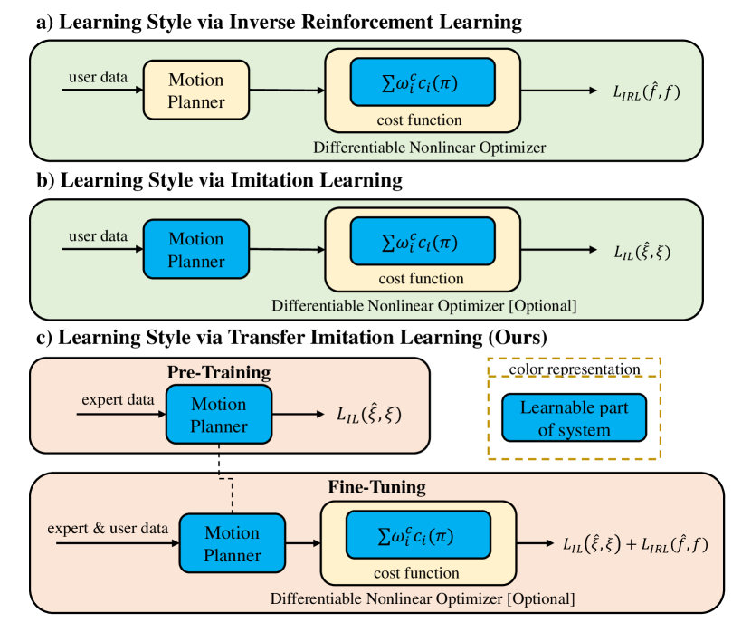
Figure 1: Approaches to learning driving style can generally be categorized into two main groups: (a) The first class involves using inverse reinforcement learning to learn cost functions from demonstrations. (b) The second class involves using imitation learning to learn neural networks from demonstrations. (c) Nevertheless, these methods often encounter overfitting and poor generalization challenges when learning from sparse user demonstrations. To address these challenges, we propose an approach termed Personalized Planning via Transfer Imitation Learning (PP-TIL).

For data-driven personalization planning, Fig. 1 presents a comparative analysis between our proposed approach and prior methodologies. Existing approaches can be broadly categorized into two main groups: inverse reinforcement learning-based methods and imitation learning-based methods. For methods grounded in inverse reinforcement learning, certain studies in general-purpose planning [5, 6] explore style learning within complex urban environments. Conversely, other researchers utilize inverse reinforcement learning to acquire the linear-structure cost function, thereby enabling user-style autonomous driving [3, 7, 8]. These methodologies learn user-style cost functions from demonstrations to achieve personalized planning. Besides, the methods based on imitation learning [9, 10, 11, 12, 13, 14] often aim to obtrain a human-like driving strategy by learning from large-scale human expert demonstrations. The above methods have demonstrated promising results in their original tasks. However, when it comes to personalized planning, user demonstrations are expensive and limited in quantity. In the experiment (refer to Table. V), we find that fine-tuning the pre-trained model using the above methods on sparse user demonstrations resulted in degraded planning performance and poor generalization of driving styles.

To address the above challenges, we propose an effective transfer imitation learning method based on the four design principles proposed in gapBoost [15]. Here’s how we integrate these principles: Rule 1: We construct a weighted experience loss based on the imitation learning method. Rule 2: We assign equal weights to the samples in the same domain to avoid highly expensive computations. Rule 3: We adjust the sampling probabilities of source and target datasets by modifying the ratio of expert samples to user samples in the input batch. Since the amount of expert data vastly exceeds the amount of user data, there is a higher expectation value for the weights assigned to user samples. Rule 4: We utilize the inverse reinforcement learning method to construct the regularization term, which measures the style gap by calculating the style feature expectation error of the trajectory. We implicitly learn the weight of each sample by adjusting the model parameters.

We conduct numerous experiments on the proposed method. We apply the proposed method to evaluate the performance of various fine-tuning structures. Our method outperforms all baseline methods in both style error and planning performance. It is worth noting that the baseline approaches achieved worse results than the pre-trained model, while our approach achieved superior performance. Additionally, through the sufficient update steps, we find that the fine-tuning architecture integrating a neural network with a differentiable nonlinear optimizer yields the best performance.

In summary, this paper makes the following three contributions:

• In this paper, we propose a novel approach called the instance-based transfer imitation learning method for achieving personalized planning within intricate urban settings.

• The proposed method effectively transfers knowledge from expert data, addressing the challenges of overfitting and poor generalization stemming from the sparse user demonstrations.

• The effectiveness of the proposed method is demonstrated through a multitude of experiments. Experimental results indicate that our method achieves superior user style approximation and planning performance enhancement.

II Related Work

II-A Machine Learning-based Planning for Autonomous Driving

In the urban structured scene, some traditional trajectory planning methods based on optimization have been widely used in industry and academia [16, 17, 18, 19]. However, these hand-designed methods tend to have weak decision-making capabilities, cannot handle long-tail scenarios, and do not improve with increasing data. In recent years, more and more works have proved the potential of planning methods based on machine learning in handling a large number of different autonomous driving urban scenarios [9, 10, 20, 11, 12, 13, 14]. But machine learning-based planning often has difficulty interpreting its output, and when it encounters out-of-distribution situations it is likely to lead to dangerous actions.

Some hybrid frameworks combine the machine learning-based approach and optimization-based approach [21, 22]. Although it nicely combines the strengths of the machine learning-based approach and the optimization-based approach, it requires large amounts of human data to train.

In the case of sparse user demonstrations, it is difficult for the previous method to obtain a sufficiently safe policy while learning styles, and there are problems of overfitting and poor generalization. To address these issues, this paper proposed personalized planning via transfer imitation learning, which is based on pre-training and fine-tuning framework. It can learn style from user data and improve the performance of planning.

II-B Personalized Planning for Autonomous Driving

Personalized planning stands as a crucial element in enhancing the user experience. Some optimization-based approaches [23, 24, 25] tend to focus solely on specific scenarios or tasks such as lane changes and obstacle avoidance. Moreover, certain studies on user style learning [3, 7, 8] frequently employ the Maximum Entropy Inverse Reinforcement Learning (MaxEnt-IRL) [26] method to learn a cost function for modeling the user’s driving style. However, applying this method to complex urban scenes poses significant challenges. Furthermore, while the general-purpose planning approach considers style learning within complex urban scenarios [5, 6], it cannot utilize data for continuous enhancement of planning performance.

It often proves challenging for these endeavors to concurrently accomplish vital aspects of both planning tasks. These include personalized planning for complex urban scenarios and the ongoing enhancement of planning performance through data utilization. This work addresses the issues of sparse user data and data-driven planning by transferring knowledge from expert data.

II-C Instance-Based Transfer Learning

In the context of personalized planning tasks in autonomous driving scenarios, the data from the expert domain and user domain exhibit strong similarities. In this case, the instance-based transfer learning approach emerges as a promising solution. Several case-based transfer learning methods employ the calculation of sample weights to facilitate effective sample transfer [27, 28, 28, 29, 30, 15]. Furthermore, some endeavors concentrate on screening valid samples from either the target or source domain [31, 32].

Inspired by these methods, we devised an effective transfer imitation learning method. Through data classification remove invalid entries. Additionally, our method implicitly adjusts sample weights via sample sampling probability and model parameter learning, thus circumventing the computational overhead associated with explicit sample weight calculation.

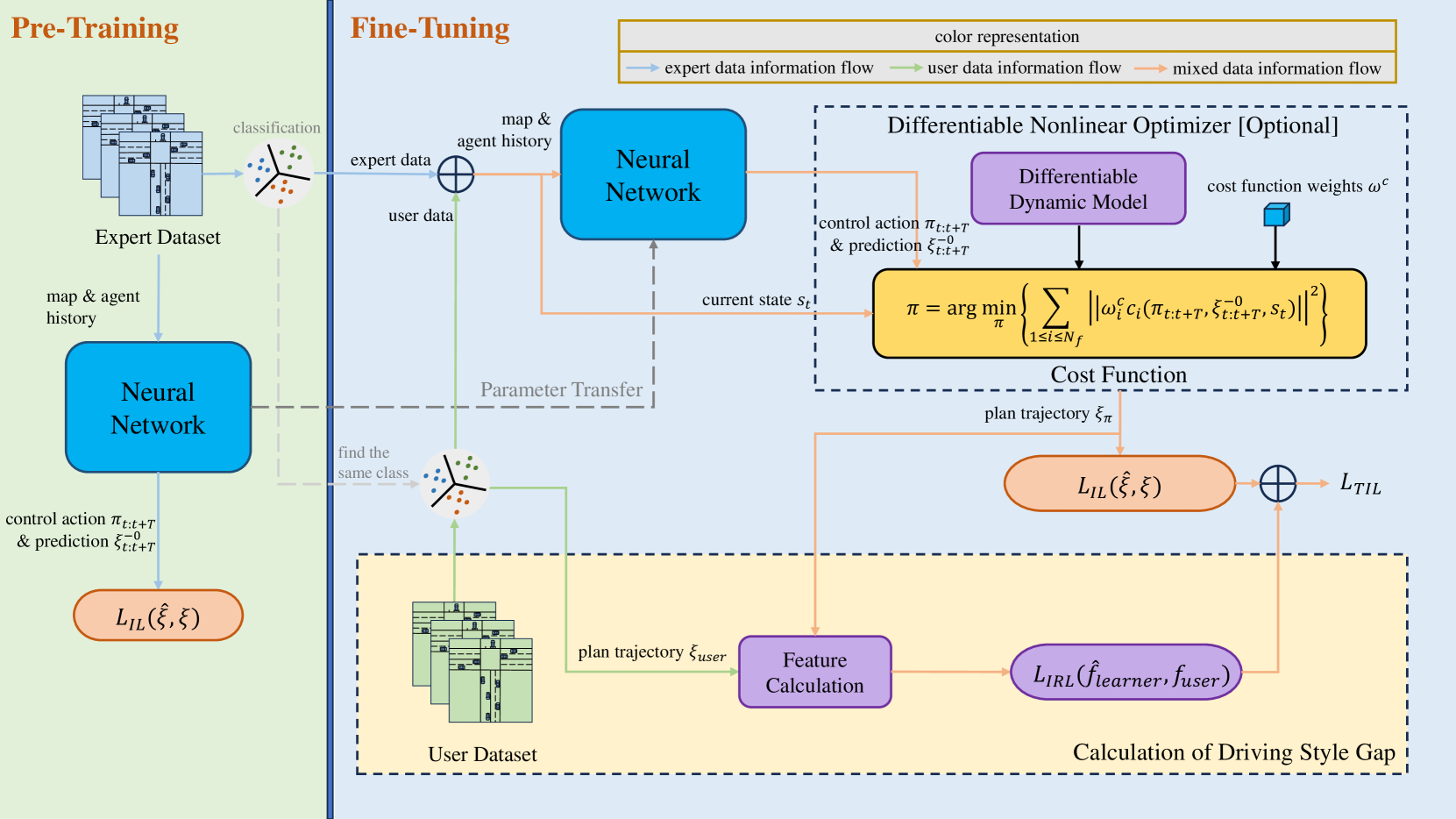
Figure 2: Personalized planning framework based on transfer imitation learning. For the specific structural design of the neural network module shown in the figure, we refer to DIPP [22]. During the pre-training stage, we train the neural network using extensive expert data. In the fine-tuning phase, we initialize the neural network with the pre-trained parameters and employ a combination of expert and user data as input batches to the model. Additionally, the differentiable motion planner module can be optionally utilized at the output side of the neural network for end-to-end fine-tuning. We leverage the maximum entropy inverse reinforcement learning method to construct $\mathcal{L}_{IRL}$. This term aiming to match the user trajectory feature expectation and learn the user trajectory style. And $\mathcal{L}_{IL}$ serves to minimize the experience error of trajectories, thereby ensuring the effectiveness of the planning.

III Personalized Planning via Transfer Imitation Learning

III-A Problem Formulation

We assume the current time step is $t$. The agent state at the current time is represented as $\bm{s}_{t}=[x_{t},y_{t},\theta_{t},v_{t}]$, where $(x_{t},y_{t})$ is two-dimensional space coordinate, $\theta_{t}$ is heading angle, and $v_{t}$ is velocity. The trajectory $\xi_{0:t}$ is represented as a set of discrete points $\{s_{0},...,s_{t}\}$. The model predicts the future trajectory of agent $i$ for the next $T$ time steps, and it’s represented as $\hat{\xi}^{i}_{t:t+T}$. The output of the neural network is the control action sequence and denoted as ${\Pi}^{m}_{t:t+T}(m={1,...,N_{m}})$, where $N_{m}$ is the number of multi-modal combinations. Specifically, the selected optimal control action sequence is denoted as ${\pi}_{t:T}$. All learnable parameters are denoted as $\omega$, including the neural network parameters $\omega^{n}$ and the cost function weights $\omega^{c}$.

III-B Pre-Training with Large-Scale Expert Data

III-B1 Differentiable Kinematic Model

To obtain a planning trajectory that satisfies the kinematic constraints, the neural network outputs the control action $u_{t}=\{a_{t},\delta_{t}\}$ (where $a_{t}$ is acceleration and $\delta_{t}$ is steering angle) and the trajectory is calculated through the kinematic model:

$$\pi_{t:t+T} =\begin{bmatrix}u_{t}&\dots&u_{T}\end{bmatrix}^{\intercal}$$ (1)

$$\hat{\xi}^{0}_{t:t+T} =\psi(s_{t},\pi_{t:t+T})$$ (2)

where the $\psi$ represents the kinematic model. In this work, we adopt the differentiable kinematic bicycle model in [22].

III-B2 Neural Network

In the pre-training stage of imitation learning, we adopt the same structure as DIPP [22]. The pre-training loss is summarized as follows:

$$\mathcal{L}_{IL}=\lambda_{1}\mathcal{L}_{prediction}+\lambda_{2}\mathcal{L}_{score}+\lambda_{3}\mathcal{L}_{imitation}$$ (3)

where $\lambda_{i}(i=1,2,3)$ is the weight that scales the different loss terms.

For imitation loss, the control action sequence is used to calculate the trajectory of the autonomous vehicle through the kinematic model, and the distance from the ground truth is measured to form the imitation loss:

$$\mathcal{L}_{imitation}=\mathrm{smooth}L1(\psi(s_{t},\pi_{t:t+T})-\xi^{0}_{t:t+T})$$ (4)

where $\xi^{0}_{t:t+T}$ represents the ground truth trajectories in the dataset.

III-C Fine-Tuning with Instance-Based Transfer Imitation Learning

III-C1 Differentiable Nonlinear Optimization

In the fine-tuning stage, we use differentiable nonlinear optimization [33] to refine the control action sequence of the output of the pre-training model. To be specific, the optimization process is formulated as follows:

$${\pi}^{*}=\arg\min_{\pi}\ \frac{1}{2}\sum_{i}^{N_{f}}\|\omega_{i}^{c}c_{i}(\pi)\|^{2}$$ (5)

where $c_{i}(\pi)$ is the cost function of the control action sequence $\pi$, $\omega_{i}^{c}(i=1,...,N_{f})$ is the scaling weight and $N_{f}$ is the number of cost functions $c_{i}(\pi)$. The trajectory features are designed based on autonomous driving planning tasks, which include travel efficiency, ride comfort, lane departure, traffic rules, and most importantly safety [22].

III-C2 Maximum Entropy Inverse Reinforcement Learning

. To solve the ambiguity of multiple solutions and the randomness of expert behavior, we adopt Maximum Entropy Inverse Reinforcement Learning (MaxEnt-IRL) to learn the weights [26]:

$$P(\xi|\omega^{c})=\frac{\exp(-c(\xi|\omega^{c}))}{Z(\omega^{c})}$$ (6)

where $Z(\omega^{c})$, called partition function, equals to $\sum_{\xi}\exp(-c(\xi|\omega^{c}))$. According to this function, plans with equivalent costs have equal probability.

The Max-Ent IRL method optimizes the weight $\omega^{c}$ by maximizing the probability of the human demonstration trajectories $\xi\in D$. The gradient of this optimization problem can be computed as follows [26]:

$$\nabla\mathcal{L}_{IRL}=\mathbb{E}_{P(\xi|\omega^{c})}[\hat{f}_{i}]-f_{i}$$ (7)

However, calculating the expectation in Eq. 7 through sampling is challenging. One possible approximation of the expected feature values is to compute the feature values of the most likely trajectory [3]. To extend to neural network parameter updates, instead of using feature errors as gradients, we approximate the solution by performing gradient descent on the following objective:

$$\mathcal{L}_{IRL}\approx\frac{1}{N_{f}}\sum_{i=1}^{N_{f}}{\beta_{i}|\hat{f}_{i}-f_{i}|}$$ (8)

where $f$ is the feature of the trajectory and $\beta$ is the corresponding scaling factor. We refer to [22] for the design of seven metrics to describe trajectory features. The name and scaling factor of each feature are shown in Table I.

TABLE I: The feature weights in inverse reinforcement learning

features	Acc(lat)	Acc(lon)	Jerk(lat)	Jerk(lon)	Efficiency	Road Offset	Safety
scaling	0.008	0.008	0.004	0.01	0.004	0.0005	0.01

• Acc(lat): lateral acceleration, Acc(lon): longitudinal acceleration.

III-C3 Instance-Based Transfer Imitation Learning

By adhering to the design principles delineated in gapBoost [15], we propose an instance-based transfer imitation learning algorithm. By amalgamating Eq. 8 and Eq. 3, we formulate the optimization objectives of instance-based transfer imitation learning as follows:

$$\mathcal{L}_{TIL}^{\alpha}=\mathcal{L}_{IL}+\alpha\mathcal{L}_{IRL}$$ (9)

The parameter $\alpha>0$ denotes the scaling factor of the $L_{IRL}$ term, utilized for adjusting the weight of the regularization component within the optimization objective. $L_{IRL}$ serves as a regularization term aimed at reducing the performance disparity across domains, which accomplishes style approximation by aligning the feature distribution expectation of the input sample with that of the user sample. In practical implementation, we utilize this regularization term along with an imitation learning term to update all learnable parameters $\omega$.

TABLE II: The classification rules for planning trajectory

classification rule	rule1	rule2
Stationary	$max(speed)<2m/s$	$Displacement<2m$
Straight	$abs(\delta_{heading})<\frac{\pi}{6}$	–
Turn	$abs(\delta_{heading})<-\frac{\pi}{6}$	$abs(\delta_{heading})>\frac{\pi}{6}$
	$LateralDisplacement>0$	$LateralDisplacement<0$

Algorithm 1 Personalized planning via Transfer Imitation Learning (PP-TIL)

notation: model parameters $\omega$, class $k$ expert dataset $\mathcal{D}_{expert}^{k}$, class $k$ user dataset $\mathcal{D}_{user}^{k}$, class $k$ expert samples $X_{expert}^{k}$, class $k$ user samples $X_{user}^{k}$, class $k$ input batch $X_{input}^{k}$, expert proportion in a batch $\mathcal{P}$, batch size $\mathcal{N}$, update step $\mathcal{S}$, class number $K$.
initialize: $\omega^{n}\leftarrow$ initialize parameter via PreTraining (Eq. 3)
[optional] joint differentiable nonlinear optimizer
Classification: a rule-based approach is used to classify the dataset into $K$ classes

for $step\in\{1,...,\mathcal{S}\}$ do

       for $k\in\{1,...,K\}$ do

             $X_{expert}^{k}\leftarrow$ sample $\mathcal{N}*\mathcal{P}$ data frames from $\mathcal{D}_{expert}^{k}$ $X_{user}^{k}\leftarrow$ sample $\mathcal{N}*(1-\mathcal{P})$ data frames from $\mathcal{D}_{user}^{k}$ $X_{input}^{k}\leftarrow$ concatenate $X_{expert}^{k}$ and $X_{user}^{k}$ $\mathcal{L}_{IRL}\leftarrow$ build IRL loss based on $X_{input}^{k}$ and $\mathcal{D}_{user}^{k}$ $\omega^{*}\leftarrow$ update via $X_{input}^{k}$ and Eq. 9

       end for

      

end for

return $\omega^{*}$

As shown in Algo. 1, We delineate the detailed process of instance-based transfer imitation learning. Initially, we categorize the dataset based on the type of planning trajectory. Refer to Table. II for the specific classification criteria. In our study, we categorize it into three classes: stationary, straight, and turn. As the stationary category lacks user style information, we exclude it during the fine-tuning phase. We sample from both the expert and user data within the remaining categories to construct the mixed input batch at each iteration. Simultaneously, we utilize the corresponding user data category to formulate the IRL regularization term. Finally, we feed the batch data into the model for gradient computation and update the parameters using $\mathcal{L}_{TIL}$.

IV Experiments

IV-A Experiment Settings

IV-A1 Dataset Settings

We train and validate the approaches on the Waymo Open Motion Dataset (WOMD) [34], a large-scale real-world driving dataset focus on urban driving scenarios. We set a 7-second time window to segment the 20-second driving scene into frames, which includes a 2-second horizon for historical observation and a 5-second horizon for future prediction and planning. The window slides in 10 timesteps from the beginning of the scene and produces segments of 14 frames. In the experiment, we obtain 916808 frames from the scene, of which 80% is used for training, while the rest is used for open-loop testing. Furthermore, the trajectory feature vector is computed based on the feature terms and scaling coefficients outlined in Table. I. Subsequently, 10,000 samples are extracted from the test set for clustering using K-means, resulting in three clustering centers. Finally, we select the 64 sample frames nearest to each center point to obtain three distinct user datasets representing different styles.

In addition, based on the feature items and scaling factors in Table I, we compute trajectory feature vectors. Subsequently, we extract 10,000 samples from the test set and apply the k-means clustering algorithm to obtain three clustering centers. Finally, we select the 64 sample frames closest to each cluster center to form three distinct datasets, which we use as user data for training. The expectation of user style features is presented in Table. III.

TABLE III: The style feature expectations of the different users

class	name	Acc(lat)	Acc(lon)	Jerk(lat)	Jerk(lon)	Efficiency	Road Offset	Safety
Straight	User1	0.03089	0.00030	0.00620	0.00417	0.03358	0.00671	0.00127
	User2	0.10873	0.00549	0.00001	0.00166	0.04181	0.00465	0.00073
	User3	0.00126	0.00030	0.00333	0.00123	0.02078	0.00678	0.00002
Turn	User1	0.04955	0.16039	0.05637	0.01409	0.03583	0.02098	0.00207
	User2	0.26095	0.11560	0.02183	0.01154	0.04054	0.02136	0.00141
	User3	0.00807	0.01139	0.03083	0.01343	0.03805	0.01948	0.00305

• Acc(lat): lateral acceleration, Acc(lon): longitudinal acceleration.

IV-A2 Metrics

In the experiment, this paper designs collision rate, red light, off route, planning error, and prediction error referring to DIPP [22]. Additionally, we define the “style error” metric, calculated as shown in Eq. 8. The “style error” is evaluated by computing the mean absolute error between the trajectory features produced by the model and those from the user demonstration, thus assessing the style similarity.

IV-A3 Implementation Details

The pre-trained model undergoes five epochs of training on the expert dataset. Throughout training, the step size of the nonlinear optimizer is fixed at 0.4, and the number of iterations is set to 2. All experiments in this paper adhere to the same initial parameter settings as follows: a batch size of 64, a neural network learning rate of 1e-5, and a linear weight learning rate for the cost function of 1e-3.

IV-B Open-Loop Test

TABLE IV: Hand-Crafted cost function weights

cost function	speed	acc	jerk	steer	rate	pos	head	traffic	safety
weights	0.1	0.5	0.1	0.01	0.5	0.5	5	10	10

• The specific details of the cost function can be found in DIPP [22].

TABLE V: Compare fine-tuning methods in open-loop testing

Fine-Tuning Structure	Parameter Update (Updated Part / Method)	In Domain			Out of Domain
		Plan error ($m$)		Style	Red light	Off route	Collision	Prediction error ($m$)		Style
		@1s	@3s	error	(%)$\downarrow$	(%)$\downarrow$	(%)$\downarrow$	ADE@5s	FDE@5s	error
NN	None	0.2044	0.5994	0.08321	0.12	0.42	3.14	0.6857	1.7015	0.06892
	NN / $\mathcal{L}_{IL}$	0.1991	0.4637	0.06793	0.78	0.42	3.80	0.7086	1.7273	0.06545
	NN / $\mathcal{L}_{IRL}$	0.2124	0.7064	0.02050	0.22	0.42	3.86	0.7000	1.7154	0.05255
	NN / $\mathcal{L}_{TIL}$ (Ours)	0.2038	0.5076	0.03950	0.19	0.42	2.87	0.6753	1.6579	0.04448
NN&CF	None	0.5861	4.0462	0.07570	0.01	0.27	9.05	0.6857	1.7015	0.05911
	CF / Human	0.2136	0.8657	0.01748	0.02	0.39	1.94	–	–	0.03389
	CF / $\mathcal{L}_{IL}$	0.2162	0.8579	0.03073	0.02	0.40	3.90	–	–	0.04329
	CF / $\mathcal{L}_{IRL}$ (LfD [3])	0.4131	1.4857	0.04460	0.01	0.42	6.06	–	–	0.04070
	CF / $\mathcal{L}_{TIL}$ (Ours)	0.2725	0.9494	0.01695	0.02	0.39	2.82	–	–	0.04247
	NN / $\mathcal{L}_{IL}$ + CF / Human	0.2284	0.8787	0.01724	0.01	0.37	1.95	0.7158	1.7255	0.03355
	NN / $\mathcal{L}_{IRL}$ + CF / Human	0.2135	0.8843	0.01522	0.02	0.38	1.92	0.7573	1.7725	0.03312
	NN / $\mathcal{L}_{TIL}$ (Ours) + CF / Human	0.2224	0.8455	0.01675	0.02	0.38	1.77	0.6865	1.6682	0.03342
	NN&CF / $\mathcal{L}_{IL}$ (DIPP [22])	0.2458	0.8199	0.02173	0.03	0.35	4.69	0.7173	1.7359	0.03796
	NN&CF / $\mathcal{L}_{IRL}$	0.5738	1.7309	0.04342	0.01	0.42	8.69	0.6919	1.6929	0.05499
	NN&CF / $\mathcal{L}_{TIL}$ (Ours)	0.2568	0.7813	0.02063	0.02	0.36	3.58	0.6837	1.6756	0.03585

• None: no fine-tuning, NN: neural network, CF: cost function, NN&CF: joint neural network and cost function.

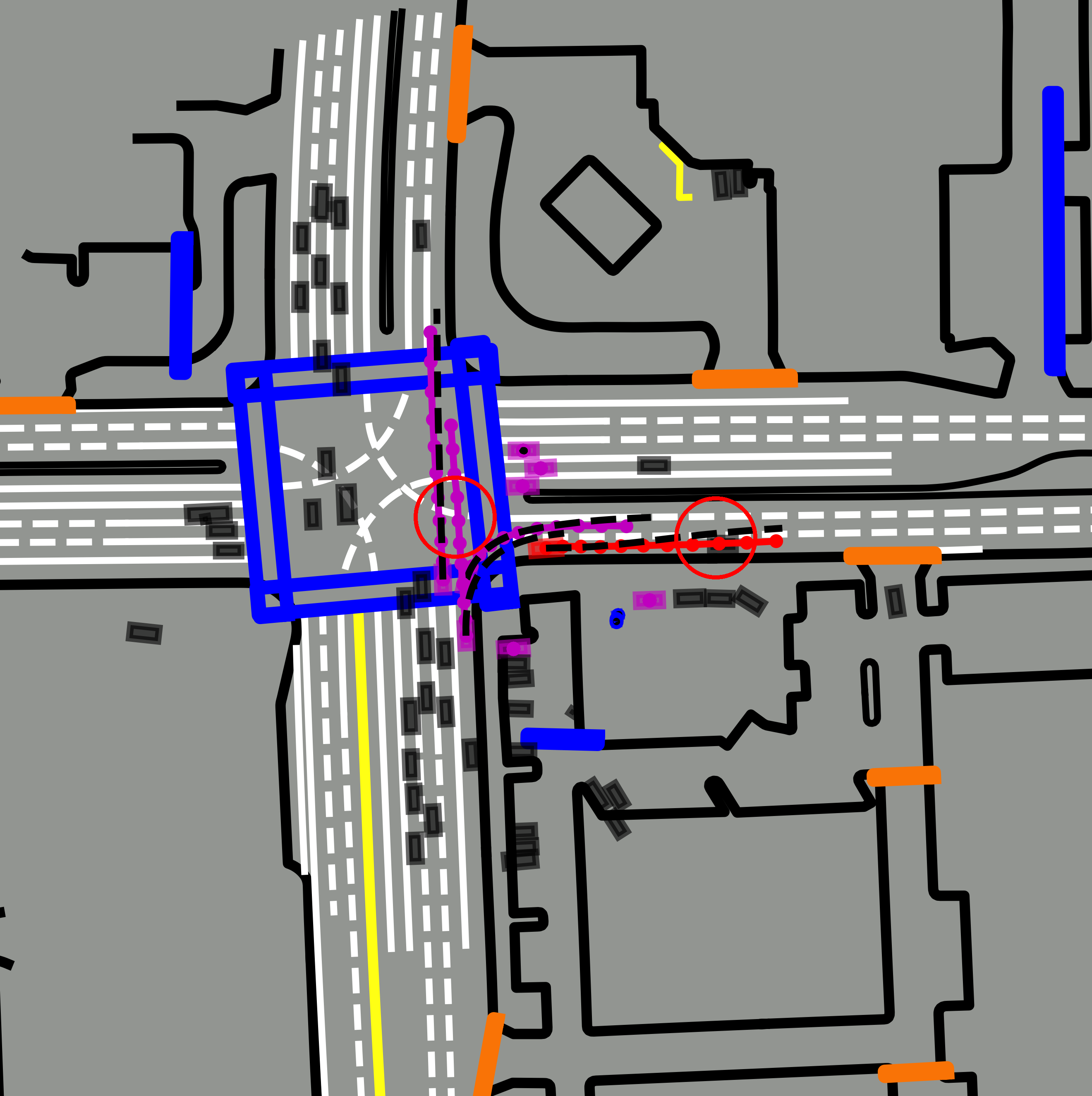
(a) Pre-Training Model

(b) (NN) NN / Ours

(c) (NN&CF) NN&CF / Ours

Figure 3: Visualization of the final results. We compare the user’s real trajectory with the output trajectory of three different models. Different categories are visually distinguished using various colors in the diagram. The color scheme for the rectangles is depicted as follows: autonomous vehicle, predicted vehicle, other vehicle, crosswalk and speed bump. The color scheme for the lines is depicted as follows: planned trajectory, predicted trajectory and road edges. In particular, the black dotted line represents the ground-truth trajectory. The red circle in the figure aids in better distinguishing the differences between different approaches.

As depicted in Table V, we conduct comprehensive experiments involving various fine-tuning architectures and fine-tuning methods. “$\mathcal{L}_{IL}$” denotes the imitation learning method outlined in Eq. 3, while “$\mathcal{L}_{IRL}$” represents the inverse reinforcement learning method illustrated in Eq. 8. “$\mathcal{L}_{TIL}$” signifies the utilization of the transfer imitation learning method detailed in Eq. 9. Due to the low effectiveness of the methods without the pre-training process, we establish a stronger baseline to demonstrate the superiority of our approach. Specifically, all experiments listed in the table are conducted based on the pre-trained model, and we compare the performance of different methods during the fine-tuning stage. We update each model 100 times and repeat each fine-tuning method thrice, presenting the average results in the table. “Human” denotes manually adjusting the weights of the cost function, as specified in Table IV. In this experiment, our method involves mixing expert data and user data in a 50% ratio, with the $\alpha$ of the $\mathcal{L}_{TIL}$ set to 100. We perform the in-domain evaluation on the user dataset and the out-of-domain evaluation on the test dataset.

The experimental results are presented in Table V demonstrate that the performance of baseline methods is worse after fine-tuning than before because of overfitting, while the proposed approach achieves fine-tuning performance improvements. In addition, our method effectively considers both user behavior imitation within the domain and style generalization outside the domain. Notably, our method achieves competitive planning performance, along with lower style error.

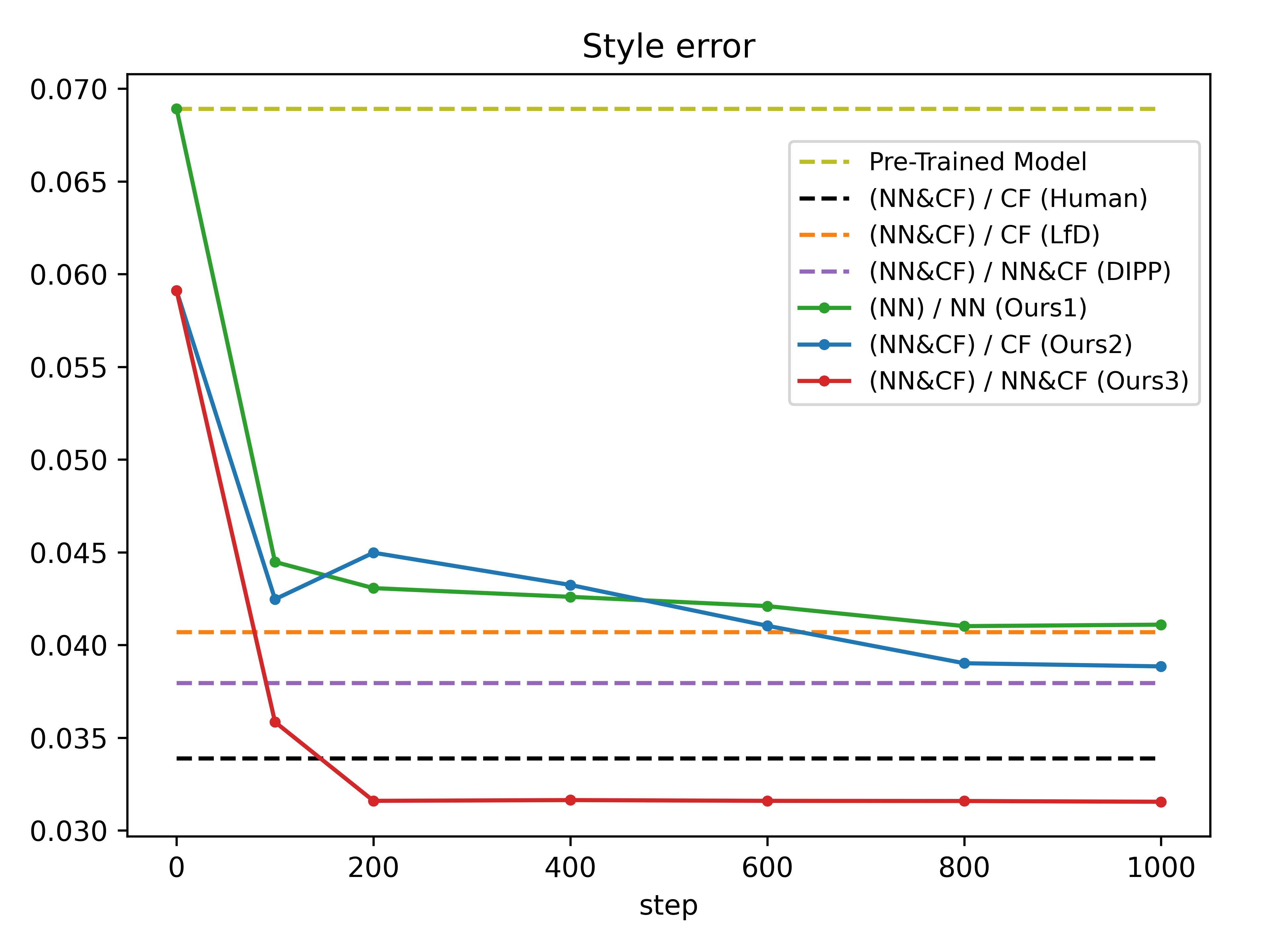
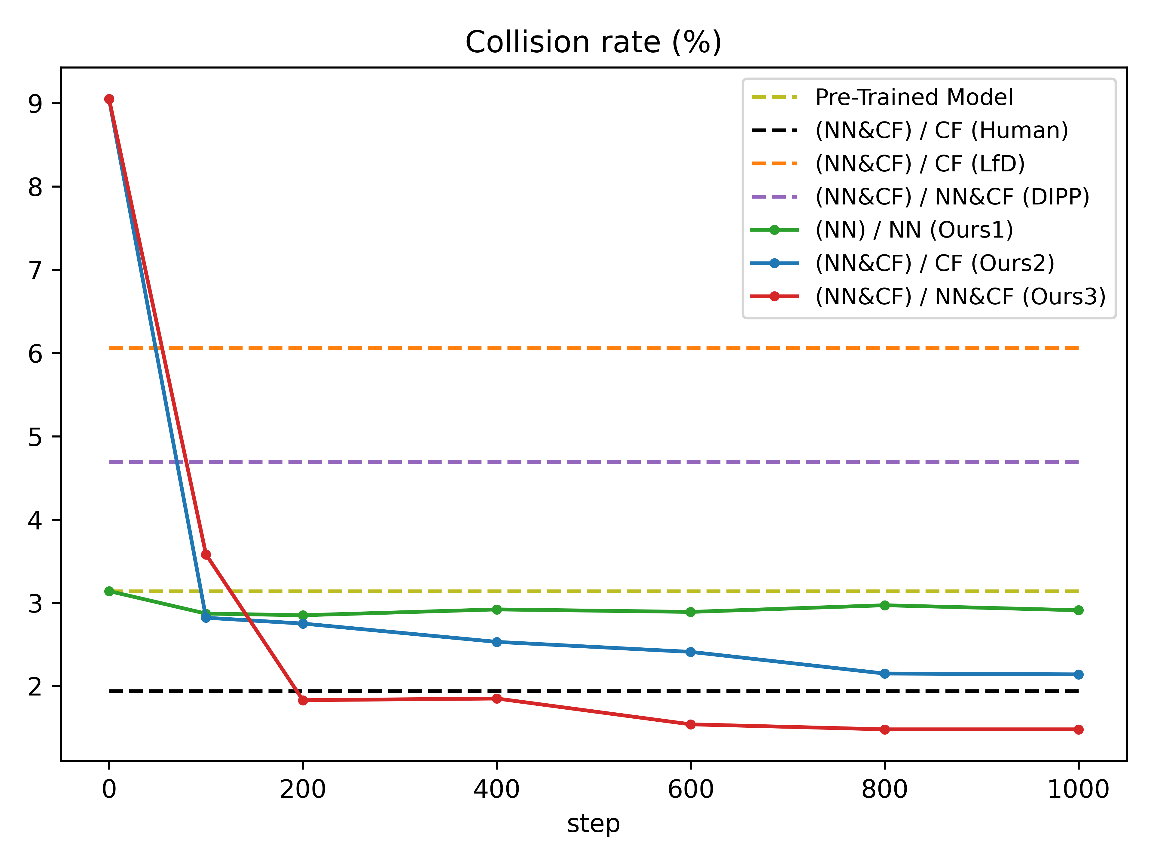
Figure 4: Comparison of different steps. The figure depicts the average values from three repeated experiments. We perform 1000 times parameter updates for each model, reducing the learning rate by half every 200 steps. The parentheses indicate the fine-tuning framework utilized, with the outer parentheses denoting the part for parameter update.

Comparison of different steps. To further evaluate whether our algorithm is prone to overfitting, we present in Fig. 4 the trends of style feature matching error and collision rate changes with the update steps across three learning structures. The curve values in the figure represent the average results obtained from three out-of-domain experiments. Due to overfitting to sparse user data, “LfD” and “DIPP” exhibit higher collision rates and poorer style generalization capability. Upon analyzing the curve trends, the final convergence outcome of the “NN&CF” framework surpasses that of the “NN” framework in two key metrics: style error and collision rate. “(NN&CF) / CF” initially converges faster. However, since the cost function solely learns linear weights, its final convergence performance is limited. “(NN&CF) / NN&CF” proves less effective when the number of update steps is small. In such cases, the linear weight of the cost function hasn’t been adequately learned, and it hasn’t adapted well to the neural network. However, with sufficient update steps, “(NN&CF) / NN&CF” achieves the best performance and even outperforms manual adjustments. This is attributed to the strong fitting ability of the neural network, which mitigates the problem of the cost function’s insufficient fitting capacity.

IV-C Ablation Study

TABLE VI: Loss ablation study

		In Domain	Out of Domain
(Fine-Tuning Structure) / Updated Part	Loss	Plan error @3s ($m$)	Prediction error ($m$) ADE@5s FDE@5s		Collision (%)	Style error
(NN) / NN	$\mathcal{L}_{IL}$	0.4814	0.6735	1.6510	3.37	0.06291
	$\mathcal{L}_{TIL}^{1}$	0.4740	0.6739	1.6524	3.23	0.05551
	$\mathcal{L}_{TIL}^{10}$	0.4792	0.6735	1.6509	3.03	0.04640
	$\mathcal{L}_{TIL}^{100}$	0.5076	0.6753	1.6579	2.87	0.04448
	$\mathcal{L}_{TIL}^{1000}$	0.5727	0.6799	1.6793	2.67	0.04144
	$\mathcal{L}_{IRL}$	0.8023	0.7050	1.7285	5.20	0.03869
(NN&CF) / NN&CF	$\mathcal{L}_{IL}$	0.6903	0.6836	1.6669	3.88	0.04003
	$\mathcal{L}_{TIL}^{1}$	0.8006	0.6949	1.6816	5.57	0.03766
	$\mathcal{L}_{TIL}^{10}$	0.7604	0.6837	1.6714	5.50	0.03800
	$\mathcal{L}_{TIL}^{100}$	0.7813	0.6837	1.6756	3.58	0.03585
	$\mathcal{L}_{TIL}^{1000}$	1.1904	0.6862	1.6788	4.85	0.04366
	$\mathcal{L}_{IRL}$	1.4948	0.7109	1.7146	5.46	0.05056

• NN: neural network, CF: cost function, NN&CF: joint neural network and cost function.

Loss ablation study. As depicted in Table VI, various losses are ablated. The input batch data for all experiments in the table consists of a 50% mixture of expert data and user data. We conduct 100 updates for each setting and present the averages of three repeated experiments. To better validate the efficacy of the loss, we only modify the loss to explore the effectiveness of the proposed method. The results indicate that the method utilizing only $\mathcal{L}_{IL}$ for parameter updates exhibits the poorest performance in the “style error” indicator and achieves the lowest approximation accuracy for user style. Conversely, the method employing only $\mathcal{L}_{IRL}$ performs inadequately on other vital planning performance metrics. $\mathcal{L}_{TIL}$ effectively balances user style approximation with the performance enhancements of the planning and forecasting modules. Additionally, we conduct parametric sensitivity experiments on the weight proportion between the $\mathcal{L}_{IL}$ and $\mathcal{L}_{IRL}$. The results indicate that $\alpha=100$ serves as a suitable trade-off between planned performance improvements and user style approximation, which tends to result in lower style error and collision rate.

TABLE VII: Mixed proportion ablation study

		In Domain	Out of Domain
(Fine-Tuning Structure) / Updated Part	Proportion	Plan error @3s ($m$)	Prediction error ($m$) ADE@5s FDE@5s		Collision (%)	Style error
(NN) / NN	$0\%$	0.5237	0.7081	1.7226	3.61	0.05684
	$25\%$	0.5086	0.6835	1.6723	2.98	0.04993
	$50\%$	0.5076	0.6753	1.6579	2.87	0.04448
	$75\%$	0.5480	0.6654	1.6452	2.95	0.04301
	$100\%$	0.5786	0.6677	1.6473	2.98	0.04488
(NN&CF) / NN&CF	$0\%$	0.5743	0.7175	1.7359	3.82	0.06404
	$25\%$	0.7509	0.6889	1.6793	3.08	0.03769
	$50\%$	0.7813	0.6837	1.6756	3.58	0.03585
	$75\%$	0.7287	0.6762	1.6581	2.93	0.03636
	$100\%$	0.8459	0.6885	1.6764	3.61	0.04460

• NN: neural network, CF: cost function, NN&CF: joint neural network and cost function, Proportion: the proportion of expert data in the mini-batch of input.

Mixed proportion ablation study. As presented in Table VII, we examine different ratios of mixing expert data to explore their influence on fine-tuning outcomes. For each setting, we conduct 100 updates and report the average of three repeated experiments. Throughout the experiment, we utilize $\mathcal{L}_{TIL}$ to update the parameters and set the $\alpha$ parameter to 100. The results indicate that when the mixing ratio of expert data is 0%, the model tends to overfit to user data, resulting in poor generalization performance since only user data is utilized. Conversely, when the mixing ratio of expert data is 100%, the planning error within the user domain increases significantly because only expert data is input. Across experiments, it is evident that the trade-off between planning performance enhancement and user style approximation is better achieved with a mixture ratio of 75%, often resulting in lower style error and collision rate.

IV-D Qualitative Results

Visualization of the final results. We utilized the three models obtained from the Fig. 4 experiment to conduct further analysis, presenting the qualitative findings in Fig. 3. The figure showcases visualizations of the three models. The trajectory duration is fixed at 5 seconds. The purple curve denotes the predicted trajectory of other cars, with the model considering only the ten nearest other cars for trajectory prediction.

V Conclusion

In this paper, we propose an instance-based transfer imitation learning approach aimed at addressing the challenge of scarcity in user domain data. We employ a pre-trained fine-tuning framework to transfer expertise from the expert domain to alleviate the data scarcity issue in the user domain. Our experimental results demonstrate that our method achieves competitive planning performance while effectively capturing the driving style of the user. At the same time, it is vital to acknowledge the limitations of this work. Firstly, we do not conduct closed-loop real-world experiments. Besides, we utilize the error of the feature expectation of the trajectory to measure user style. To better represent user driving styles or cater to user needs, it is essential to develop more appropriate methods for measuring user styles.

References

- [1] Z. Zhu and H. Zhao, “A survey of deep rl and il for autonomous driving policy learning,” IEEE Transactions on Intelligent Transportation Systems, vol. 23, no. 9, pp. 14 043–14 065, 2021.
- [2] S. Teng, X. Hu, P. Deng, B. Li, Y. Li, Y. Ai, D. Yang, L. Li, Z. Xuanyuan, F. Zhu et al., “Motion planning for autonomous driving: The state of the art and future perspectives,” IEEE Transactions on Intelligent Vehicles, 2023.
- [3] M. Kuderer, S. Gulati, and W. Burgard, “Learning driving styles for autonomous vehicles from demonstration,” in Proceedings of the IEEE international conference on robotics and automation (ICRA). IEEE, 2015, pp. 2641–2646.
- [4] M. L. Schrum, E. Sumner, M. C. Gombolay, and A. Best, “Maveric: A data-driven approach to personalized autonomous driving,” IEEE Transactions on Robotics, 2024.
- [5] S. Rosbach, V. James, S. Großjohann, S. Homoceanu, and S. Roth, “Driving with style: Inverse reinforcement learning in general-purpose planning for automated driving,” in Proceedings of the IEEE/RSJ International Conference on Intelligent Robots and Systems (IROS). IEEE, 2019, pp. 2658–2665.
- [6] S. Rosbach, V. James, S. Großjohann, S. Homoceanu, X. Li, and S. Roth, “Driving style encoder: Situational reward adaptation for general-purpose planning in automated driving,” in Proceedings of the IEEE international conference on robotics and automation (ICRA). IEEE, 2020, pp. 6419–6425.
- [7] Z. Wu, L. Sun, W. Zhan, C. Yang, and M. Tomizuka, “Efficient sampling-based maximum entropy inverse reinforcement learning with application to autonomous driving,” IEEE Robotics and Automation Letters, vol. 5, no. 4, pp. 5355–5362, 2020.
- [8] Z. Huang, J. Wu, and C. Lv, “Driving behavior modeling using naturalistic human driving data with inverse reinforcement learning,” IEEE transactions on intelligent transportation systems, vol. 23, no. 8, pp. 10 239–10 251, 2021.
- [9] M. Vitelli, Y. Chang, Y. Ye, A. Ferreira, M. Wołczyk, B. Osiński, M. Niendorf, H. Grimmett, Q. Huang, A. Jain et al., “Safetynet: Safe planning for real-world self-driving vehicles using machine-learned policies,” in Proceedings of the IEEE International Conference on Robotics and Automation (ICRA), 2022, pp. 897–904.
- [10] S. Pini, C. S. Perone, A. Ahuja, A. S. R. Ferreira, M. Niendorf, and S. Zagoruyko, “Safe real-world autonomous driving by learning to predict and plan with a mixture of experts,” in Proceedings of the IEEE International Conference on Robotics and Automation (ICRA), 2023, pp. 10 069–10 075.
- [11] Y. Hu, J. Yang, L. Chen, K. Li, C. Sima, X. Zhu, S. Chai, S. Du, T. Lin, W. Wang et al., “Planning-oriented autonomous driving,” in Proceedings of the IEEE/CVF Conference on Computer Vision and Pattern Recognition, 2023, pp. 17 853–17 862.
- [12] Z. Huang, H. Liu, J. Wu, and C. Lv, “Conditional predictive behavior planning with inverse reinforcement learning for human-like autonomous driving,” IEEE Transactions on Intelligent Transportation Systems, 2023.
- [13] J. Fu, Y. Shen, Z. Jian, S. Chen, J. Xin, and N. Zheng, “Interactionnet: Joint planning and prediction for autonomous driving with transformers,” in Proceedings of the IEEE/RSJ International Conference on Intelligent Robots and Systems (IROS). IEEE, 2023, pp. 9332–9339.
- [14] D. Hu, C. Huang, J. Wu, and H. Gao, “Pre-trained transformer-enabled strategies with human-guided fine-tuning for end-to-end navigation of autonomous vehicles,” arXiv preprint arXiv:2402.12666, 2024.
- [15] B. Wang, J. Mendez, M. Cai, and E. Eaton, “Transfer learning via minimizing the performance gap between domains,” Advances in neural information processing systems, vol. 32, 2019.
- [16] S. Sun, Z. Liu, H. Yin, and M. H. Ang, “Fiss: A trajectory planning framework using fast iterative search and sampling strategy for autonomous driving,” IEEE Robotics and Automation Letters, vol. 7, no. 4, pp. 9985–9992, 2022.
- [17] H. Fan, F. Zhu, C. Liu, L. Zhang, L. Zhuang, D. Li, W. Zhu, J. Hu, H. Li, and Q. Kong, “Baidu apollo em motion planner,” arXiv preprint arXiv:1807.08048, 2018.
- [18] Z. Ajanovic, B. Lacevic, B. Shyrokau, M. Stolz, and M. Horn, “Search-based optimal motion planning for automated driving,” in Proceedings of the IEEE/RSJ International Conference on Intelligent Robots and Systems (IROS), 2018, pp. 4523–4530.
- [19] S. Karaman and E. Frazzoli, “Sampling-based algorithms for optimal motion planning,” The International Journal of Robotics Research, vol. 30, no. 7, pp. 846–894, 2011.
- [20] T. Phan-Minh, F. Howington, T.-S. Chu, M. S. Tomov, R. E. Beaudoin, S. U. Lee, N. Li, C. Dicle, S. Findler, F. Suarez-Ruiz et al., “Driveirl: Drive in real life with inverse reinforcement learning,” in Proceedings of the IEEE International Conference on Robotics and Automation (ICRA), 2023, pp. 1544–1550.
- [21] H. Pulver, F. Eiras, L. Carozza, M. Hawasly, S. V. Albrecht, and S. Ramamoorthy, “Pilot: Efficient planning by imitation learning and optimisation for safe autonomous driving,” in Proceedings of the IEEE/RSJ International Conference on Intelligent Robots and Systems (IROS), 2021, pp. 1442–1449.
- [22] Z. Huang, H. Liu, J. Wu, and C. Lv, “Differentiable integrated motion prediction and planning with learnable cost function for autonomous driving,” IEEE Transactions on Neural Networks and Learning Systems, 2023.
- [23] Y. Yan, J. Wang, K. Zhang, Y. Liu, Y. Liu, and G. Yin, “Driver’s individual risk perception-based trajectory planning: A human-like method,” IEEE Transactions on Intelligent Transportation Systems, vol. 23, no. 11, pp. 20 413–20 428, 2022.
- [24] X. Zhang, W. Zhang, Y. Zhao, H. Wang, F. Lin, and Y. Cai, “Personalized motion planning and tracking control for autonomous vehicles obstacle avoidance,” IEEE Transactions on Vehicular Technology, vol. 71, no. 5, pp. 4733–4747, 2022.
- [25] M. R. Oudainia, C. Sentouh, A.-T. Nguyen, and J.-C. Popieul, “Personalized decision making and lateral path planning for intelligent vehicles in lane change scenarios,” in Proceedings of the IEEE 25th International Conference on Intelligent Transportation Systems (ITSC), 2022, pp. 4302–4307.
- [26] B. D. Ziebart, A. L. Maas, J. A. Bagnell, A. K. Dey et al., “Maximum entropy inverse reinforcement learning,” in Proceedings of the AAAI Conference on Artificial Intelligence, vol. 8, 2008, pp. 1433–1438.
- [27] D. Pardoe and P. Stone, “Boosting for regression transfer,” in Proceedings of the 27th International Conference on International Conference on Machine Learning, 2010, pp. 863–870.
- [28] L. Cai, J. Gu, J. Ma, and Z. Jin, “Probabilistic wind power forecasting approach via instance-based transfer learning embedded gradient boosting decision trees,” Energies, vol. 12, no. 1, p. 159, 2019.
- [29] S. Gupta, J. Bi, Y. Liu, and A. Wildani, “Boosting for regression transfer via importance sampling,” International Journal of Data Science and Analytics, pp. 1–12, 2023.
- [30] S. Jiang, H. Mao, Z. Ding, and Y. Fu, “Deep decision tree transfer boosting,” IEEE transactions on neural networks and learning systems, vol. 31, no. 2, pp. 383–395, 2019.
- [31] T. Wang, J. Huan, and M. Zhu, “Instance-based deep transfer learning,” in Proceedings of the IEEE Winter Conference on Applications of Computer Vision (WACV). IEEE, 2019, pp. 367–375.
- [32] Y. Tang, M. R. Dehaghani, P. Sajadi, and G. G. Wang, “Selecting subsets of source data for transfer learning with applications in metal additive manufacturing,” arXiv preprint arXiv:2401.08715, 2024.
- [33] L. Pineda, T. Fan, M. Monge, S. Venkataraman, P. Sodhi, R. T. Chen, J. Ortiz, D. DeTone, A. Wang, S. Anderson et al., “Theseus: A library for differentiable nonlinear optimization,” Advances in Neural Information Processing Systems, vol. 35, pp. 3801–3818, 2022.
- [34] S. Ettinger, S. Cheng, B. Caine, C. Liu, H. Zhao, S. Pradhan, Y. Chai, B. Sapp, C. R. Qi, Y. Zhou et al., “Large scale interactive motion forecasting for autonomous driving: The waymo open motion dataset,” in Proceedings of the IEEE/CVF International Conference on Computer Vision, 2021, pp. 9710–9719.