On the precise quantification of the impact of a single discretionary lane change on surrounding traffic

Abstract

Lane-changing is a critical maneuver of vehicle driving, and a comprehensive understanding of its impact on traffic is essential for effective traffic management and optimization. Unfortunately, existing studies fail to adequately distinguish the impact of lane changes from those resulting from natural traffic dynamics. Additionally, there is a lack of precise methods for measuring the spatial extent and duration of the impact of a single discretionary lane change, as well as a definitive metric to quantify the overall spatiotemporal impact. To address these gaps, this study introduces a quantitative indicator called the Corrected Travel Distance Bias (CTDB), which accounts for variable speeds due to inherent traffic dynamics, providing a more accurate assessment of lane-changing impacts. A comprehensive methodology is developed to compare vehicle trajectory data before and after lane-changing events, measuring both the magnitude and spatiotemporal extent of the lane-changing impact. The results, based on the Zen traffic data from Japan, indicate that the impact of a lane change in the target lane lasts an average of 23.8 seconds, affecting approximately 5.6 vehicles, with a CTDB value of -10.8 meters. In contrast, in the original lane, the impact lasts 25 seconds, affects 5.3 vehicles, and yields a CTDB value of 4.7 meters.

1 Introduction

Lane-changing is a critical component of traffic dynamics, significantly influencing traffic flow efficiency and road safety. Despite substantial advancements in developing algorithms for lane-changing decision making (Ali et al., 2021; Li et al., 2022; Zhang et al., 2023), trajectory planning (Zong et al., 2022; Liu et al., 2022; Gao et al., 2023; Hou et al., 2024), and lane-changing prediction (Xing et al., 2020; Ali et al., 2022; Huang et al., 2024), the magnitude that a single discretionary lane change can impact traffic has not been satisfactorily answered yet (Zheng, 2014). Precise observation and measurement underscore the need for accurate modeling of lane-changing impacts to devise effective traffic control strategies and enhance road safety measures. Consequently, exploring quantitative approaches to assess the impact of a lane change is of significant importance.

Existing studies on lane-changing impact quantification can be divided into macroscopic and microscopic approaches. Macroscopic methods evaluate the effects of lane changes from an aggregate traffic dynamics perspective, primarily focusing on traffic efficiency, safety, and fuel consumption (Jin, 2010, 2013; Feng et al., 2015; Pan et al., 2016; Li and Sun, 2017; Zhu et al., 2022). These studies specifically examine the influence of all lane-changing vehicles on the overall traffic flow. For instance, Jin (2010) introduced location-dependent lane-changing intensity variable into the fundamental diagram. Building on this, Jin (2013) developed a multicommodity kinematic wave (KW) model that treated lane-changing vehicles and non-lane-changing vehicles as separate commodities to explore their impact on traffic capacity. Feng et al. (2015) quantified the lane-changing impact by calculating the average delay using statistical analysis of simulation data. Li and Sun (2017) applied car-following and lane-changing models to assess the impact of lane changes on traffic flow rate, average vehicle speed, traffic safety, and fuel consumption in scenarios involving lane drops and moving bottlenecks. Zhu et al. (2022) proposed a cooperative merging model designed to minimize the total delay caused by merging maneuvers for all vehicles passing through the ramp merging area. However, these macroscopic methods do not provide insights at the individual vehicle level, which limits their effectiveness in detailed microscopic lane-changing decision studies.

Microscopic approaches, on the other hand, focus on the specific effects of a lane change at the level of individual vehicles, analyzing the complex behaviors and interactions of the lane-changing vehicle and its surrounding vehicles during the lane-changing process. These approaches can be further classified into three categories: instantaneous quantification, fixed spatial-temporal quantification, and dynamic impact quantification. In the category of instantaneous quantification, the Minimizing Overall Braking Induced by Lane Change (MOBIL) model, introduced by Kesting et al. (2007), utilized the anticipated acceleration of the "following vehicle in the target lane (referred to as TFV)" as an indicator of lane-changing impact to guide lane-changing decisions. Xie et al. (2019) considered the status of the lane-changing vehicle’s immediate adjacent vehicles (such as TFV) as pivotal features influencing lane-changing decisions, proposing a deep belief network-based lane-changing decision model. Hou et al. (2023) eveloped utility functions that incorporate lane-changing impacts in terms of efficiency and comfort for the TFV, aiding vehicles in deciding between maintaining longitudinal movement and executing a lane change. However, these methods primarily focus on the impact on the immediate following vehicle and provide only an instantaneous assessment of the lane-changing impact.

In the category of fixed spatial-temporal quantification, Coifman et al. (2006) introduced the concept of delay induced by a lane change and proposed a method to estimate it between two detectors, considering the distance between two detectors as the spatial extent of the lane-changing impact. Yang et al. (2019) evaluated the lane-changing impact on the immediate following vehicle using metrics such as speed change rate, braking timestamp, and time-to-collision (TTC) during the lane-changing duration. Li et al. (2020) predicted the lane-changing impact on crash risks and flow change, employing a fixed spatiotemporal impact region, assuming a fixed number of 5 TFVs affected by a single lane change for 9 seconds, with an equal impact duration for each vehicle. This assumption overlooks the fact that the impact duration may vary among different TFVs. Chen et al. (2023a, b) measured the lane-changing impact within the pre-insertion process (referred to as anticipation) by examining the difference in reaction time of the immediate TFV at the start and end moments of this anticipation process. A critical limitation of these methods is that selecting inappropriate spatial or temporal thresholds can lead to either overestimation or underestimation of the impact magnitude, failing to capture the dynamic progression of the impact.

In the category of dynamic quantification, notable contributions have been made by two key studies (Zheng et al., 2013; He et al., 2023). Zheng et al. (2013) emphasized that driver characteristics, such as reaction time and minimum spacing in Newell’s car-following model, exhibit time-dependent changes. By leveraging the relationship between the maximum passing rate and response time proposed by Chiabaut et al. (2009), they calibrated the time-dependent reaction time and assessed the lane-changing impact on the immediate follower in the target lane based on the evolving pattern of reaction time. However, this study does not specify a precise temporal or spatial range for the lane-changing impact. He et al. (2023) determined the number of vehicles affected by a lane change and the temporal range for each affected vehicle by utilizing the evolving pattern of minimum spacing. However, this method cannot differentiate between positive and negative lane-changing impacts (such as a decrease or increase in travel time), as it focuses solely on the affected duration or the number of affected vehicles.

In summary, most existing studies on the quantification of the temporal and spatial impact of a single lane change are insufficient and inaccurate (Table 1), leading to two significant research gaps. First, there has been little research distinguishing the effects induced by a lane change from those arising due to inherent traffic dynamics fluctuations, resulting in inaccuracies in lane-changing impact quantification. Second, few studies have accurately quantified the spatial extent and duration of lane-changing impact on both the original and target lanes, nor have they distinguished between positive and negative impacts. A method that addresses these gaps is urgently needed to enable more accurate lane-changing impact quantification, thereby better assisting lane-changing decisions.

Table 1: Comparative study of dynamic quantification for lane-changing impact

Methodological capabilities	Zheng et al. (2013)	He et al. (2023)	This study
Quantify the impact duration (temporal)	✗	✓	✓
Quantify the number of affected vehicles (spatial)	✗	✓	✓
Quantify the cumulative spatiotemporal impact	✗	✗	✓
Exclude the effects induced by inherent traffic dynamics	✗	✗	✓
Distinguish between positive and negative impacts	✗	✗	✓

To address these gaps, this paper presents a comprehensive methodology to precisely quantify the spatiotemporal impact of a single discretionary lane change at the vehicle level by comparing naturalistic trajectory data before and after the lane change. The main contributions of this study are as follows (Table 1):

1. Analytical Approach: We propose a naturalistic trajectory data-based analytical approach that not only offers a deterministic assessment of the cumulative spatiotemporal impact magnitude of a single lane change on upstream vehicles in both the original and target lanes, but also distinguishes between positive and negative impacts. Specifically, this method indicates whether there is a decrease or increase in travel distance during the lane-changing impact duration compared to a non-lane change condition.

2. Efficiency Metrics: We introduce two key efficiency metrics: the Travel Distance Bias (TDB) and the Corrected Travel Distance Bias (CTDB). The TDB is used to determine whether an upstream following vehicle is influenced by a lane change, while the CTDB measures the magnitude of the lane-changing impact. Unlike traditional traffic delay metrics, both TDB and CTDB accommodate fluctuating speeds due to inherent traffic dynamics, providing a more accurate quantification of the lane-changing impact.

3. Empirical Insights: Key empirical insights from Zen Traffic Dataset include: a) The temporal and spatial impact ranges of a lane change are similar in both the target and original lanes, typically lasting an average of 24 seconds and affecting approximately 5.5 vehicles; b) The cumulative spatiotemporal impact magnitude (CTDB value) shows significant differences between the target and original lanes, averaging -10.8 meters in the target lane (indicating negative efficiency) and 4.7 meters in the original lane (indicating positive efficiency).

This study provides a deeper understanding of the spatiotemporal impact of a single discretionary lane change, highlighting the differences in lane-changing impacts on different lanes. This knowledge can assist automated vehicles in making more informed lane-changing decisions.

The remainder of this paper is structured as follows: Section 2 outlines the methodology used to quantify the spatiotemporal impact of lane-changing at the individual vehicle level. Section 3 details the trajectory data used in this study, the methods for obtaining lane-changing data, and determining the precise start time of each lane change. Section 4 provides an in-depth analysis of the lane-changing impact through data examples. Finally, Section 5 concludes with a summary of the main findings and proposes directions for future research in this area.

2 Methodology

Fig. 1 illustrates a typical lane-changing scenario, where the subjective vehicle (SV) intends to change lanes, TLV and ${TFV}_{i}$ represent the leading and the $i^{th}$ following vehicles of SV in the target lane, respectively. Similarly, LV and ${FV}_{i}$ are the leading and following vehicles of SV in the original lane, respectively. $T_{SV}^{lane}$ denotes the moment when the SV crosses the lane marking, while $T_{SV}^{s}$ denotes the moment when SV initiates the lane-changing process.

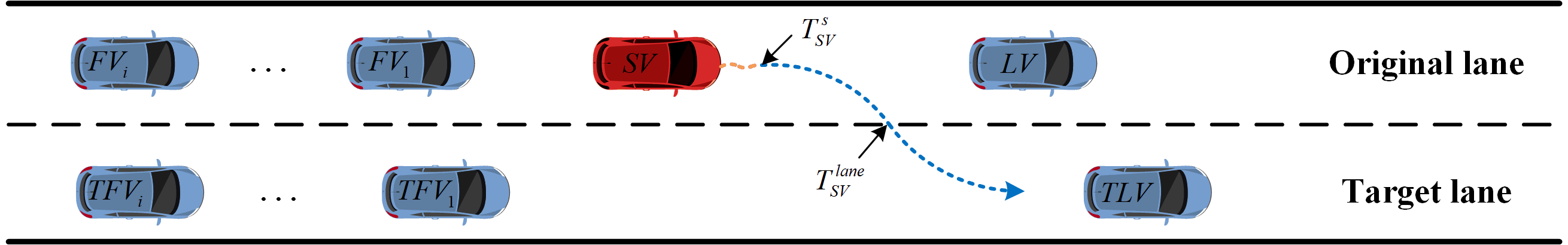
Figure 1: Illustration of a typical lane-changing scenario

The proposed approach for quantifying the lane-changing impact comprises four critical components: 1) Identifying the demarcation time, $T_{i}^{s}$, using a kinematic wave theory-based method to differentiate between potentially affected and unaffected data for each following vehicle in the target lane ($TFV_{i}$) and in the original lane ($FV_{i}$). 2) Design of an efficiency metric to detect the travel distance bias (TDB) of vehicles. 3) Establishment of two judgment criteria to determine whether the $TFV_{i}$ or $FV_{i}$ is affected by the lane change of the SV, and to determine their respective affected time duration. 4) Calculation of the overall impact magnitude of a single lane change on upstream traffic by integrating the corrected TDB (CTDB) and the duration of impact for all affected vehicles. For clarity, the main variables and parameters used in this methodology are summarized in Table 2.

Table 2: Notation List

Notation	Description
$T_{SV}^{s}$	Time at which SV initiates the lane-changing execution process
$T_{i}^{s}$	Demarcation time used to distinguish between potentially unaffected and affected data of ${TFV}_{i}$
${TDB}_{i}(k)$	Travel distance bias at the $k^{th}$ time interval, representing the delay distance of ${TFV}_{i}$ relative to TLV
${TDB}_{i}^{\ast}$	Threshold for TDB of ${TFV}_{i}$
$\Delta t$	Time interval
$\Theta_{i}(k)$	Indicator of potentially affected status of ${TFV}_{i}$ at the $k^{th}$ time interval
$\mathbf{\Theta}_{\mathit{i}}^{\mathit{f}},\mathbf{\Theta}_{\mathit{i}}^{\mathit{r}}$	Sets of $\Theta_{i}(k)$ in the potentially unaffected and affected data segments, respectively
$n_{i}^{f},n_{i}^{r}$	Number of $\Delta t$ intervals in potentially unaffected and affected data segments, respectively
$\Omega_{i}^{f\ast}$	Maximum number of consecutive occurrences of $\Theta_{i}(k)=1$ in the potentially unaffected data segment for ${TFV}_{i}$
$\mathbf{c}_{i,q}^{f},\mathbf{c}_{i,q}^{r}$	Sets of $k$ values corresponding to $\Omega_{i,q}^{f},\Omega_{i,q}^{r}$, respectively
$\mathbf{K}_{i}^{\mathit{A}}$	Set of estimated affected time intervals for ${TFV}_{i}$
$\Upsilon_{i}$	Estimated affected status of ${TFV}_{i}$
$T_{i}^{A}$	Impact duration of the SV’s lane change on ${TFV}_{i}$
${CTDB}_{i}(k)$	Corrected Travel Distance Bias by integrating ${TDB}_{i}(k)$ with a correction factor $\delta_{i}(k)$
$\delta_{i}(k)$	Correction factor of CTDB
$w_{i}^{A}$	Impact magnitude of the SV’s lane change on ${TFV}_{i}$, i.e., the sum of ${CTDB}_{i}(k)$ over the impact duration
$N_{A}$	Total number of affected TFVs
$W^{A}$	Total impact magnitude of the SV’s lane change on all affected ${TFV}_{i}$
$T^{A}$	Overall duration of impact from the SV’s lane change on traffic flow

2.1 Determining $T_{i}^{s}$ using kinematic wave theory

To illustrate the methodology, consider ${TFV}_{i}$ (the same methodology applies to ${FV}_{i}$). Since the exact moment when ${TFV}_{i}$ is initially affected by the SV’s lane change cannot be precisely determined, we predefine a demarcation time $T_{i}^{s}$ to distinguish between potentially unaffected and affected data for ${TFV}_{i}$. Specifically, this time mark helps differentiate the data: prior to $T_{i}^{s}$ represents potentially unaffected data, while post $T_{i}^{s}$ represents potentially affected data. We then assess whether the SV’s lane change impacts ${TFV}_{i}$ by comparing these two sets of data. $T_{i}^{s}$ should be as closely aligned as possible with the actual moment when ${TFV}_{i}$ begins to be affected.

Fig. 2 illustrates an instance of the extracted lane-changing data. The red and black lines represent the trajectory curves of the SV and ${TFV}_{10}$, respectively, with the black dot marking the moment when the SV initiates the lane-changing process ($T_{SV}^{s}$). If $T_{SV}^{s}$ is considered as $T_{i}^{s}$, it becomes apparent that the potentially unaffected data of ${TFV}_{i}$ diminishes with the distance from the SV. In such a situation, there is almost no potentially unaffected data available for ${TFV}_{10}$, indicating that using $T_{SV}^{s}$ as the demarcation time might not provide sufficient potentially unaffected data for ${TFV}_{i}$ located further from the SV. This limitation can significantly affect the accuracy of the lane-changing impact analysis.

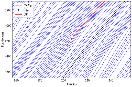
Figure 2: Trajectories from an extracted lane-changing instance

To ensure a balanced availability of potentially unaffected and affected data for each ${TFV}_{i}$ and to make the determination of $T_{i}^{s}$ more accurate, we propose a refined method based on kinematic wave theory. Due to the SV’s lane change causing ${TFV}_{i}$ to decelerate, a deceleration wave propagates upstream. The time it takes for this kinematic wave to travel between two adjacent vehicles ($t_{w}$) can be calculated as (Holland, 1998; Qin et al., 2021):

$$t_{w}=\frac{h}{v-c}=\left[\frac{dV}{dh}\right]^{-1}=\left[V^{\prime}(h)\right]^{-1}$$ (1)

where $h$ and $v$ represent the equilibrium spacing and speed, respectively, and $c$ is the wave speed relative to the road, which is a positive value. $V(h)$ denotes the equilibrium speed-spacing function, i.e., $v=V(h)$. Referring to (Qin et al., 2021), we can obtain:

$$[V^{\prime}(h)]^{-1}=h^{v}$$ (2)

where $h^{v}$ represents the derivative of $h$ with respect to $v$. $T_{i}^{s}$ is then calculated by:

$$T_{i}^{s}=T_{SV}^{s}+\sum_{j=1}^{i}t_{w,j},\quad i\geq 1$$ (3)

where $t_{w,j}$ represents the time required for the kinematic wave to propagate between vehicle ${TFV}_{j}$ and its preceding vehicle ${TFV}_{j-1}$. According to Eqs. (1) and (2), $t_{w,j}$ equals $h_{j}^{v}$, and can be calibrated using real trajectory data based on the lower order Newell model (Newell, 2002):

$$x_{j}(t+\tau_{j})=x_{j-1}(t)-d_{j}$$ (4)

where $\tau_{j}$ and $d_{j}$ represent the reaction time and minimum space of vehicle $j$, respectively. $x_{j}$ and $x_{j-1}$ denote the positions of vehicles $j$ and $j-1$, respectively. In the Newell model, the relationship between $h_{j}$ and $v$ at equilibrium is given by:

$$h_{j}=d_{j}+v\tau_{j}$$ (5)

From Eq. (5), $h_{j}^{v}$ is obtained as $\tau_{j}$, thus $t_{w,j}=\tau_{j}$, and $T_{i}^{s}=T_{SV}^{s}+\sum_{j=1}^{i}\tau_{j}$. The parameter $\tau_{j}$ of the Newell model is calibrated to minimize the discrepancy between the observed trajectories and those predicted by the Newell model, using the preceding vehicle’s position data as input. The objective function for the calibration is the sum of squared errors (SSE):

$$(\tau_{j}^{*},d_{j}^{*})=\underset{(\tau_{j},d_{j})}{\text{argmin}}\sum_{t\in T_{\text{all}}^{j}}(x_{j}(t)-x_{j}^{\prime}(t))^{2}$$ (6)

where $x_{j}^{\prime}(t)$ represents the predicted position of vehicle $j$ at time $t$, and $T_{\text{all}}^{j}$ represents the total time that vehicle $j$ is within the selected trajectory set. Parameters were calibrated for each ${TFV}_{j}$ independently, with bounds set as $\tau_{j}\in[0.1,5]$ and $d_{j}\in[0.1,10]$.

2.2 Designing the Travel Distance Bias (TDB) metric

Fig. 3 illustrates vehicle trajectories in the target and original lanes before and after a lane change. Consider Fig. 3a as an illustration, where $D_{2}^{f}$, $D_{2}^{r}$, and $s_{2}^{r}$ represent the distances between ${TFV}_{2}$ and TLV before $T_{2}^{s}$ and after $T_{2}^{s}$, and the distance between ${TFV}_{2}$ and ${TFV}_{1}$ after $T_{2}^{s}$, respectively. The blue, orange, and green lines depict $D_{2}^{f}$, $D_{2}^{r}$, and $s_{2}^{f}$, respectively. It is observed that $D_{2}^{r}$ changes continuously after $T_{2}^{s}$, while $s_{2}^{r}$ remains relatively stable. This stability aligns with the Newell model, which suggests that the trajectory of a following vehicle tends to mimic that of the vehicle directly in front of it. Consequently, in a car-following scenario, the distance between a vehicle and its immediately preceding vehicle typically fluctuates slightly around the equilibrium spacing, leading to minimal distance variation over short time intervals. Therefore, we focus on the change in $D_{i}$ (distance between ${TFV}_{i}$ and TLV) rather than $s_{i}$ (distance between ${TFV}_{i}$ and ${TFV}_{i-1}$) to formulate an efficiency index that reflects the lane-changing impact, known as the travel distance bias (TDB), calculated as:

$${TDB}_{i}(k)=\int_{T_{i}^{s}+(k-1)\Delta t}^{T_{i}^{s}+k\Delta t}\Delta V_{i}(t)\,dt$$ (7)

$$\Delta V_{i}(t)=v_{{TFV}_{i}}(t)-v_{{TLV}}(t)$$ (8)

where $v_{{TFV}_{i}}(t)$ and $v_{{TLV}}(t)$ represent the speeds of ${TFV}_{i}$ and TLV at time $t$, respectively. The TDB measures the relative delay distance of ${TFV}_{i}$ compared to TLV over each time interval $\Delta t$. A negative value indicates that ${TFV}_{i}$ travels a shorter distance than TLV, while a positive value suggests a longer distance.

At the macroscopic level, traditional traffic delay is typically defined as the difference between actual and ideal travel times. The ideal travel time assumes vehicles maintain a constant speed, either at their maximum speed (i.e., free flow speed) or at their non-affected speed within the study area (Xu et al., 2020; Kodupuganti and Pulugurtha, 2023). If TDB were defined similarly, $v_{TLV}$ in Eq. (8) would be considered constant, serving as an ideal reference.

However, at the microscopic level, TLV’s speed varies due to the influence of preceding vehicles. Without disturbances from the SV’s lane change, the TFVs’ state changes in response to the TLV’s fluctuating speed. If TDB were defined traditionally, these variations could be incorrectly attributed to the SV’s influence. Our proposed method accounts for the dynamic nature of traffic at the microscopic level, ensuring a more precise assessment of the SV’s impact.

Fig. 3b shows a comparable scenario for FVs in the original lane, where FVs might accelerate post $T_{i}^{s}$ to close the gap with the LV, suggesting that the SV’s lane change could potentially enhance efficiency for FVs.

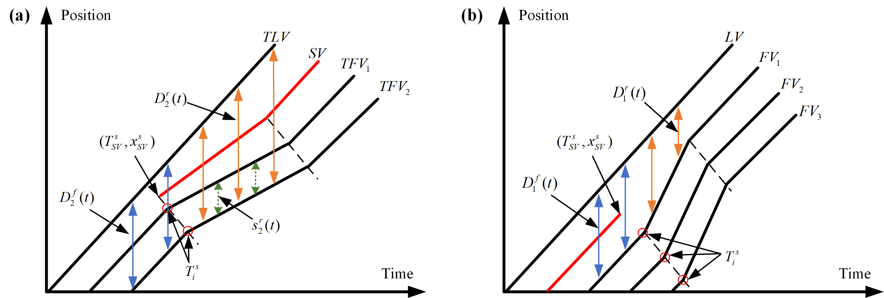
Figure 3: Schematic diagram of vehicle trajectories before and after a lane change: (a) TFVs and (b) FVs

2.3 Establishing judgment criteria for determining affected time of ${TFV}_{i}$

In this subsection, we outline the procedure for determining the affected time of ${TFV}_{i}$. It is important to note that this approach is also applicable to ${FV}_{i}$. In segments potentially unaffected by external influences such as SV’s lane change, ${TFV}_{i}$ maintains an equilibrium speed. However, speed fluctuations around this equilibrium speed may still occur. These fluctuations result in $\Delta V_{i}(k)$ not consistently equaling zero, indicating that ${TDB}_{i}(k)$ might also deviate from zero in these potentially unaffected segments. This deviation could also be attributed to noise in the vehicle trajectory data. To accurately determine whether ${TFV}_{i}$ is affected, it is crucial to analyze ${TDB}_{i}(k)$ in potentially unaffected data segments and establish a TDB threshold, denoted as ${TDB}_{i}^{*}$.

Given that ${TDB}_{i}(k)$ can be positive or negative when unaffected by a lane change, aggregating these values without differentiation could lead to inaccuracies in ${TDB}_{i}^{*}$. Therefore, we separate positive and negative ${TDB}_{i}(k)$ values in the potentially unaffected data segment as follows:

$$\mathbf{TDB}_{i}^{-}=\left\{TDB_{i}(k)\,|\,TDB_{i}(k)<0,\,k\in[1,n_{i}^{f}]\right\}$$ (9)

$$\mathbf{TDB}_{i}^{+}=\left\{TDB_{i}(k)\,|\,TDB_{i}(k)\geq 0,\,k\in[1,n_{i}^{f}]\right\}$$ (10)

$$n_{i}^{f}=\left\lfloor\frac{T_{i}^{s}-T_{i}^{lb}}{\Delta t}\right\rfloor$$ (11)

where $\mathbf{TDB}_{i}^{-}$ and $\mathbf{TDB}_{i}^{+}$ are the sets of ${TDB}_{i}(k)<0$ and ${TDB}_{i}(k)\geq 0$ in the potentially unaffected data segment, respectively. $T_{i}^{lb}$ represents the lower time boundary of the extracted trajectory data of ${TFV}_{i}$. $n_{i}^{f}$ represents the total number of $\Delta t$ intervals in the potentially unaffected data segment, specifically contained within the time range $[T_{i}^{lb},T_{i}^{s}]$. The symbol $\left\lfloor\bullet\right\rfloor$ represents the rounding down operation.

The formulas for calculating the means ($\mu_{i}^{+}$, $\mu_{i}^{-}$) and standard deviations ($\sigma_{i}^{+}$, $\sigma_{i}^{-}$) of these sets are given by:

$$\mu_{i}^{+}=\frac{1}{m_{i}}\sum_{{TDB}_{i}(k)\in\mathbf{TDB}_{i}^{+}}{TDB}_{i}(k)$$ (12)

$$\sigma_{i}^{+}=\sqrt{\frac{1}{m_{i}}\sum_{{TDB}_{i}(k)\in\mathbf{TDB}_{i}^{+}}{({TDB}_{i}(k)-\mu_{i}^{+})}^{2}}$$ (13)

$$\mu_{i}^{-}=\frac{1}{(n_{i}^{f}-m_{i})}\sum_{{TDB}_{i}(k)\in\mathbf{TDB}_{i}^{-}}{TDB}_{i}(k)$$ (14)

$$\sigma_{i}^{-}=\sqrt{\frac{1}{n_{i}^{f}-m_{i}}\sum_{{TDB}_{i}(k)\in\mathbf{TDB}_{i}^{-}}{({TDB}_{i}(k)-\mu_{i}^{-})}^{2}}$$ (15)

$$m_{i}=\left|\mathbf{TDB}_{i}^{+}\right|$$ (16)

where $\mu_{i}^{-}$ and $\mu_{i}^{+}$ represent the means of $\mathbf{TDB}_{i}^{-}$ and $\mathbf{TDB}_{i}^{+}$, respectively. $\sigma_{i}^{-}$ and $\sigma_{i}^{+}$ represent the standard deviations of $\mathbf{TDB}_{i}^{-}$ and $\mathbf{TDB}_{i}^{+}$, respectively. $m_{i}$ represents the number of values in $\mathbf{TDB}_{i}^{+}$.

The TDB threshold (${TDB}_{i}^{*}$) is defined as:

$${TDB}_{i}^{*}=\begin{cases}[\mu_{i}^{+}-\sigma_{i}^{+},\mu_{i}^{+}+\sigma_{i}^{+}],&\text{if }TDB_{i}(k)\geq 0\\ [\mu_{i}^{-}-\sigma_{i}^{-},\mu_{i}^{-}+\sigma_{i}^{-}],&\text{if }TDB_{i}(k)<0\end{cases}$$ (17)

The potentially affected status of ${TFV}_{i}$ at the $k^{th}$ time interval is defined as:

$$\Theta_{i}(k)=\begin{cases}1,&\text{if }TDB_{i}(k)\notin TDB_{i}^{*}\\ 0,&\text{otherwise}\end{cases}$$ (18)

where $\Theta_{i}$ is a binary variable, with values 1 and 0 representing potentially affected and unaffected statuses, respectively. The discrete calculation of TDB may cause $\Theta_{i}(k)$ to oscillate frequently between 0 and 1 within short time durations, which may not accurately reflect the actual driving characteristics. Additionally, disturbances unrelated to the SV’s lane change may cause large fluctuations in the speed of ${TFV}_{i}$ during certain time intervals, resulting in unexpected occurrences of $\Theta_{i}(k)=1$ in the potentially unaffected data segment. Thus, solely relying on a TDB threshold to determine whether ${TFV}_{i}$ is affected is insufficient.

To address these issues, we introduce a new discriminant index, $\Omega_{i}^{f*}$, which considers the maximum duration of the potential state $\Theta_{i}(k)=1$ in the potentially unaffected data segment, as given by:

$$\Omega_{i}^{f*}=\max(\Omega_{i,1}^{f},\Omega_{i,2}^{f},\ldots,\Omega_{i,q}^{f},\ldots),\quad q=1,2,3,\ldots$$ (19)

where $\Omega_{i,q}^{f}$ represents number of occurrences $\Theta_{i}(k)=1$ for the $q^{th}$ consecutive sequence of vehicle $i$ in the potentially unaffected data segment. A consecutive sequence is defined as consecutive occurrences of $\Theta_{i}(k)=1$.

This index helps confirm that the ${TFV}_{i}$ is affected only when the number of consecutive occurrences of $\Theta_{i}(k)=1$ exceeds $\Omega_{i}^{f*}$. By applying $\Omega_{i}^{f*}$, we can adjust these occurrences in both the potentially unaffected and affected data segments. Specifically, any duration of consecutive occurrence of $\Theta_{i}(k)=1$ that does not exceed the threshold set by $\Omega_{i}^{f*}$ is reclassified as $\Theta_{i}(k)=0$. This ensures that all $\Theta_{i}(k)$ values in the potentially unaffected data segment are equal to 0. The pseudocode of calculating $\Omega_{i}^{f*}$ and adjusting $\Theta_{i}^{f}(k)$ by applying $\Omega_{i}^{f*}$ is summarized in Algorithm 1.

Input: $\mathbf{\Theta}_{i}^{f}$

Output: $\Omega_{i}^{f\ast}$, $\mathbf{\Theta}_{i}^{f}$

1 begin

2       $\mathbf{K}_{i}^{f}=\{k\mid\mathbf{\Theta}_{i}^{f}(k)==1,k\in[1,n_{i}^{f}]\}$;

3       $z_{1}=1$, $q=1$;

4       while $z_{1}\leq\text{length}(\mathbf{K}_{i}^{f})$ do

5             $z_{2}=1$;

6             while $z_{2}\leq\text{length}(\mathbf{K}_{i}^{f})-z_{1}$ and $\mathbf{K}_{i}^{f}(z_{1})+z_{2}==\mathbf{K}_{i}^{f}(z_{1}+z_{2})$ do

7                   $z_{2}=z_{2}+1$;

8                  

9             end while

10            if $z_{2}\geq 1$ then

11                   $\mathbf{c}_{i,q}^{f}=\mathbf{K}_{i}^{f}(z_{1}:1:z_{1}+z_{2}-1)$;

12                   $\Omega_{i,q}^{f}=\textit{length}(\mathbf{c}_{i,q}^{f})$;

13                   $q=q+1$;

14                  

15             end if

16            $z_{1}=z_{1}+z_{2}$;

17            

18       end while

19      $\Omega_{i}^{f\ast}=\max(\Omega_{i,1}^{f},\Omega_{i,2}^{f},\ldots,\Omega_{i,q}^{f},\ldots)$;

20       $\mathbf{C}_{i}^{f}=\{\mathbf{c}_{i,1}^{f},\cdots,\mathbf{c}_{i,q}^{f},\cdots\}$;

21       for each $\mathbf{c}_{i,q}^{f}\subseteq\mathbf{C}_{i}^{f}$ do

22             if $\Omega_{i,q}^{f}\leq\Omega_{i}^{f\ast}$ then

23                   for each $k\in\mathbf{c}_{i,q}^{f}$ do

24                         $\mathbf{\Theta}_{i}^{f}(k)=0$;

25                        

26                   end for

27                  

28             end if

29            

30       end for

31      $\mathbf{\Theta}_{i}^{f}=\{\mathbf{\Theta}_{i}^{f}(k)\mid k\in[1,n_{i}^{f}]\}$;

32      

33 end

34

Algorithm 1 Calculation of $\Omega_{i}^{f\ast}$ and adjustment of $\Theta_{i}^{f}(k)$ by applying $\Omega_{i}^{f\ast}$

We employ a method analogous to Algorithm 1 to process the data following time $T_{i}^{s}$, referred to as the potentially affected data segment:

$$\Omega_{i}^{r}=\left\{\Omega_{i,1}^{r},\Omega_{i,2}^{r},\ldots,\Omega_{i,q}^{r},\ldots\right\},\quad q=1,2,3,\ldots$$ (20)

where $\Omega_{i,q}^{r}$ represents number of occurrences of $\Theta_{i}(k)=1$ for the $q^{th}$ consecutive sequence of vehicle $i$ in the potentially affected data segment.

Based on the threshold ($\Omega_{i}^{f\ast}$), the estimated affected time intervals $\mathbf{t}_{\mathbf{i},\mathbf{q}}^{\mathbf{A}}$ of ${TFV}_{i}$ can be determined as:

$$\mathbf{t}_{\mathbf{i},\mathbf{q}}^{\mathbf{A}}=\begin{cases}\mathbf{c}_{i,q}^{r},&\text{if }\Omega_{i,q}^{r}>\Omega_{i}^{f\ast}\\ \emptyset,&\text{otherwise}\end{cases}$$ (21)

where $\mathbf{c}_{i,q}^{r}$ represents the sets of $k$ values corresponding to $\Omega_{i,q}^{r}$. The detailed calculation of $\mathbf{c}_{i,q}^{r}$ can be found in Algorithm 1.

The union of these intervals across all $q$ is given by:

$$\mathbf{K}_{i}^{A}=\bigcup\mathbf{t}_{\mathbf{i},\mathbf{q}}^{\mathbf{A}}$$ (22)

The criterion for determining whether $TFV_{i}$ is affected by the lane change is defined as:

$$\Upsilon_{i}=\begin{cases}1,&\text{if }\mathbf{K}_{i}^{A}\neq\emptyset\\ 0,&\text{otherwise}\end{cases}$$ (23)

where $\Upsilon_{i}$ is a binary variable where a value of 1 indicates that $TFV_{i}$ is affected, and 0 indicates it is unaffected.

The impact duration of the SV’s lane change on $TFV_{i}$ is calculated as:

$$T_{i}^{A}=t_{i}^{e}-t_{i}^{s}$$ (24)

with

$$t_{i}^{s}=T_{i}^{s}+\left(\min{\left(\mathbf{K}_{i}^{A}\right)}-1\right)\cdot\Delta t$$ (25)

$$t_{i}^{e}=T_{i}^{s}+\max{\left(\mathbf{K}_{i}^{A}\right)}\cdot\Delta t$$ (26)

where $t_{i}^{s}$ and $t_{i}^{e}$ are the affected start time and affected end time of ${TFV}_{i}$, respectively.

Specifically, $T_{i}^{A}$ represents the duration between the last affected time and the start affected time of $TFV_{i}$. For clarity, Table 3 provides a numerical example illustrating the process of determining $\Upsilon_{i}$ and $T_{i}^{A}$.

Table 3: Numerical Example of Determining $\Upsilon_{i}$ and $T_{i}^{A}$

Variables	Potentially unaffected segment	Potentially affected segment
$\mathbf{\Theta}_{i}$	$\mathbf{\Theta}_{i}=\{0,1,0,1,1,0,0,1,1,1,0,1,1,0\}$
$n_{i}^{f},n_{i}^{r}$	$n_{i}^{f}=6$	$n_{i}^{r}=8$
$\mathbf{\Theta}_{i}^{f},\mathbf{\Theta}_{i}^{r}$	$\mathbf{\Theta}_{i}^{f}=\{0,1,0,1,1,0\}$	$\mathbf{\Theta}_{i}^{r}=\{0,1,1,1,0,1,1,0\}$
$\Omega_{i,q}^{f},\Omega_{i,q}^{r}$	$\Omega_{i,1}^{f}=1,\Omega_{i,2}^{f}=2$	$\Omega_{i,1}^{r}=3,\Omega_{i,2}^{r}=2$
$\mathbf{c}_{i,q}^{f},\mathbf{c}_{i,q}^{r}$	$\mathbf{c}_{i,1}^{f}=\{2\},\mathbf{c}_{i,2}^{f}=\{4,5\}$	$\mathbf{c}_{i,1}^{r}=\{8,9,10\},\mathbf{c}_{i,2}^{r}=\{12,13\}$
$\Omega_{i}^{f\ast}$	2
$\mathbf{t}_{\mathbf{i},\mathbf{q}}^{\mathbf{A}}$	-	$\mathbf{t}_{\mathbf{i},\mathbf{1}}^{\mathbf{A}}=\{8,9,10\},\mathbf{t}_{\mathbf{i},\mathbf{2}}^{\mathbf{A}}=\emptyset$
$\mathbf{K}_{i}^{A}$	-	$\{8,9,10\}$
$\Upsilon_{i}$	1
$T_{i}^{A}$	$3\Delta t$

2.4 Calculating the overall impact magnitude of the SV’s lane change

Based on the judgment criteria established in section 2.3, we define the Corrected Travel Distance Bias (CTDB) to accurately quantify the magnitude of the lane-changing impact. The CTDB incorporates ${TDB}_{i}(k)$ with a correction factor term, $\delta_{i}(k)$, designed to exclude the effects induced by inherent traffic dynamics fluctuations unrelated to the SV’s lane change. This consideration is not addressed in methods based on calibrating the evolving pattern of reaction time or minimum spacing (Zheng et al., 2013; He et al., 2023). The CTDB is defined as:

$${CTDB}_{i}(k)={TDB}_{i}(k)-\delta_{i}(k)$$ (27)

where $\delta_{i}(k)$ is defined as:

$$\delta_{i}(k)=\begin{cases}\mu_{i}^{-}-\sigma_{i}^{-}&\text{if }TDB_{i}(k)<\mu_{i}^{-}-\sigma_{i}^{-}\\ \mu_{i}^{-}+\sigma_{i}^{-}&\text{if }\mu_{i}^{-}+\sigma_{i}^{-}<TDB_{i}(k)<0\\ \mu_{i}^{+}-\sigma_{i}^{+}&\text{if }0<TDB_{i}(k)<\mu_{i}^{+}-\sigma_{i}^{+}\\ \mu_{i}^{+}+\sigma_{i}^{+}&\text{if }TDB_{i}(k)>\mu_{i}^{+}+\sigma_{i}^{+}\\ TDB_{i}(k)&\text{otherwise}\end{cases}$$ (28)

The impact magnitude of the SV’s lane change on ${TFV}_{i}$ is calculated as the sum of ${CTDB}_{i}(k)$ over the impact duration, given by:

$$w_{i}^{A}=\sum_{k\in\mathbf{K}_{i}^{A}}{{CTDB}_{i}(k)}$$ (29)

To mitigate random effects, we consider that if two consecutive vehicles remain unaffected by the lane change, i.e., $\Upsilon_{i}=0$ and $\Upsilon_{i+1}=0$, it suggests that the influence of the deceleration wave has been effectively absorbed or dissipated by these vehicles, reducing the likelihood of further impact on upstream vehicles. This helps determine the total number of affected ${TFV}_{i}$, denoted as $N_{A}$:

$$N_{A}=\begin{cases}i-1,&\text{if }\Upsilon_{i}+\Upsilon_{i+1}==0\\ N,&\text{otherwise}\end{cases}\;,\quad i=1,2,\ldots,N-1$$ (30)

where $N$ represents the number of ${TFV}_{i}$ within the extracted trajectory data.

The total impact magnitude of the SV’s lane change on all ${TFV}_{i}$ is then calculated as:

$$W^{A}=\sum_{i=1}^{N_{A}}w_{i}^{A}\cdot\Upsilon_{i}$$ (31)

Let $t_{\text{last}}$ denotes the difference between the affected end time of the last affected TFV ($t_{E}$) and the affected start time of the first affected TFV ($t_{S}$), given by:

$$t_{\text{last}}=t_{E}-t_{S}$$ (32)

with

$$t_{E}=T_{N_{A}}^{s}+\max\left(\mathbf{K}_{N_{A}}^{A}\right)\cdot\Delta t$$ (33)

$$t_{S}=T_{initial}^{s}+\min\left(\mathbf{K}_{initial}^{A}\right)\cdot\Delta t$$ (34)

where $T_{N_{A}}^{s}$ and $T_{initial}^{s}$ are the demarcation times for distinguishing between potentially unaffected and affected data of the ${N_{A}}^{th}$ TFV and the first affected TFV, i.e., ${TFV}_{N_{A}}$ and ${TFV}_{initial}$. $\mathbf{K}_{N_{A}}^{A}$ and $\mathbf{K}_{initial}^{A}$ are the sets of estimated affected time intervals for ${TFV}_{N_{A}}$ and ${TFV}_{initial}$, respectively.

Since $t_{last}$ may be greater than or less than the maximum $T_{i}^{A}$, the impact duration of the SV’s lane change on the target lane is calculated as:

$$T^{A}=\max{\left(t_{\text{last}},\max\limits_{1\leq i\leq N_{A}}{(T_{i}^{A})}\right)}$$ (35)

It is worth noting that Eqs. (1)-(35) are explained using TFVs as an example, but all methods are equally applicable to FVs.

3 Data Preparation

3.1 The Zen Traffic Data

For a comprehensive analysis of the temporal and spatial impact of a single lane change on upstream traffic, access to extensive data is essential. Commonly used traffic trajectory datasets such as HighD and NGSIM are constrained by their limited road lengths—420 meters for HighD, and 640 meters for US101 and 500 meters for I80 in NGSIM, respectively. These constraints limit their effectiveness for in-depth analysis. To overcome this limitation, this study utilizes the Zen Traffic Data (ZTD) from Japan, which is known for its extensive coverage and is thus more suitable for examining the comprehensive effects of lane changes.

The ZTD dataset consists of vehicle travel data collected from two road segments in Japan, specifically Routes #4, #11, and #13. Each segment encompasses two main lanes (a driving lane and a passing lane) and one ramp lane. As illustrated in Fig. 4, the data comprises both free-flow traffic and congested traffic, enabling a comprehensive analysis of the lane-changing impact across various traffic conditions. The driving lane typically serves slower-moving traffic, while the passing lane accommodates faster-moving vehicles. The data collection durations were as follows: 5 hours for each of the first two segments and 6 hours for the third segment, with recordings taken at 0.1-second intervals. The lengths of the segments for Routes #4, #11 and #13 are 2 km, 1.6km and 2.7 km, respectively. Key data attributes include vehicle ID, datetime, vehicle type, velocity, laneID, kilopost (distance from the downstream endpoint of the expressway route), and geographic coordinates (latitude and longitude). It is important to note that traffic in Japan moves on the left, and the kilopost readings decrease as the vehicle travels along the route.

To enhance the reliability of the speed within the dataset, we apply a filtering method as described by Montanino and Punzo (2015). This method helps to smooth the speed profiles of the trajectories, thereby reducing the impact of random noise and improving the accuracy of our analysis.

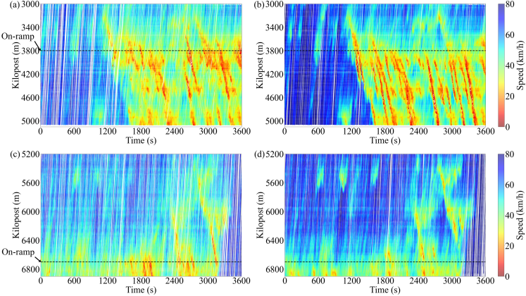
Figure 4: Vehicle trajectories of different routes: (a) Ikeda Route #11 (F001) driving lane; (b) Ikeda Route #11 (F001) passing lane; (c) Wangan Route #4 (F001) driving lane; (d) Wangan Route #4 (F001) passing lane (from https://zen-traffic-data.net/english/outline/)

3.2 Lane-changing data extraction

To quantify the impact of the SV’s lane change on upstream traffic and analyze the relationship between the lane-changing impact and traffic flow status, we extract the lane-changing data involving SV and its surrounding vehicles based on the following criteria:

Criterion 1: Data from all vehicles in all lanes are extracted within a 50-second window before and after $T_{SV}^{lane}$ and within a 500-meter range before and after the position corresponding to $T_{SV}^{lane}$. The $T_{SV}^{lane}$ moment is determined by a change in the laneID attribute of the SV.

Criterion 2: This study focuses exclusively on instances of single discretionary lane changes. Mandatory lane changes, such as merges and diverges, as well as consecutive lane changes, such as those spanning two or more lanes continuously, or overtaking followed by a return to the original lane, are excluded.

Criterion 3: To exclude the interactive influence of other lane changes, only instances where no upstream vehicle of the SV changes lanes into either the target or original lanes after SV changes lanes.

After applying these criteria, a total of 228 effective instances of lane-changing vehicles and their surrounding vehicles are obtained.

3.3 Determining lane-changing start time

Accurately determining $T_{SV}^{s}$ is crucial for quantifying the lane-changing impact of the SV. However, due to the lack of $T_{SV}^{s}$ in raw ZTD dataset, we employ the following steps to determine it:

Step 1: Calculate the lateral coordinate of vehicles. First, extract data for lane keeping vehicles within the left lane (driving lane) from the Zen Traffic Data. These vehicles maintain a constant laneID, indicating no lane changes. Second, calculate the average longitude and latitude data of these extracted lane keeping vehicles to represent the centerline of the driving lane. Third, utilize the latitude and longitude data of vehicles along with the centerline data to calculate the lateral distance of each vehicle from the centerline of the driving lane at each time point. This distance serves as the lateral position of the vehicle.

Step 2: Obtain the lane-changing start time $\mathbf{T_{SV}^{s}}$. $T_{SV}^{s}$ is typically determined by analyzing the oscillation frequency of the lateral position or lateral speed (Dong et al., 2021; Shangguan et al., 2022; Venthuruthiyil and Chunchu, 2022). In this study, we adopt the method based on the lateral position. Specifically, after a certain instant, the lateral position of SV ceases to oscillate and instead consistently decreases or increases. This instant is defined as $T_{SV}^{s}$.

Fig. 5 shows two examples of identifying the start time of the lane changes based on the aforementioned method.

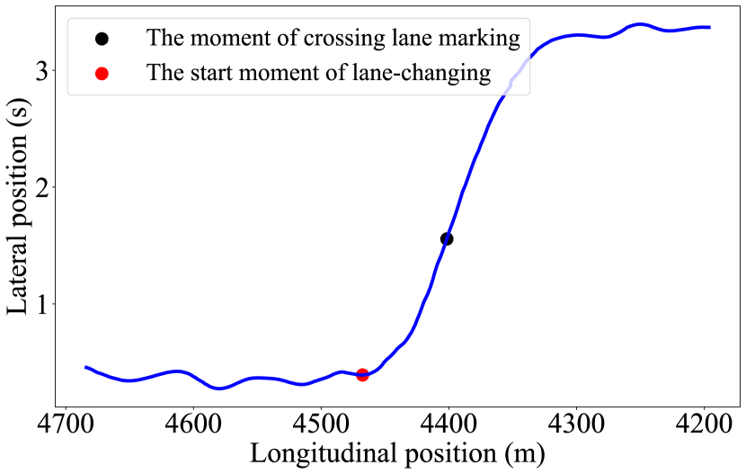
(a)

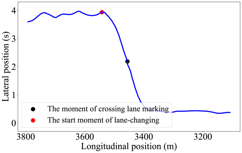
(b)

Figure 5: Two examples of identifying the lane-changing start time

4 Case study of lane-changing impact

To demonstrate the effectiveness of our proposed methodology, we applied it to a case study that analyzes the impacts of a lane change using the extracted lane-changing instances from Section 3. We set the time interval, $\Delta t$, to 0.5 seconds. A larger interval might neutralize the positive and negative effects of fluctuations, while a smaller interval might not adequately capture changes in TDB, leading to an inaccurate representation of traffic dynamics.

4.1 Visualization of lane-changing impact quantification process

To effectively visualize and quantify the impact of a lane change, we selected a specific lane-changing instance as illustrated in Fig. 6. Fig. 6(a) details the process for ${TFV}_{1}$, while Fig. 6(b) illustrates the process for ${FV}_{1}$. Taking ${TFV}_{1}$ as an example, Fig. 6(a) shows the TDB, potential affected status ($\Theta_{1}$), and estimated affected status ($\Upsilon_{1}$) at each time interval. Colored regions in the lower part of the diagram represent $\Theta_{i}=1$ or $\Upsilon_{i}=1$, while white regions indicate $\Theta_{i}=0$ or $\Upsilon_{i}=0$. Using the first judgment criterion defined in Eqs. (17) and (18), we determined the potential affected status of ${TFV}_{1}$ at each time interval, as shown in the second subfigure of Fig. 6(a). The $\Omega_{i}^{f\ast}$ was observed to be 4. After the demarcation time $T_{1}^{s}$, the estimated affected status is adjusted according to the second judgment criterion outlined in Eqs. (21)-(23), depicted in the third subfigure of Fig. 6(a). The impact duration on ${TFV}_{1}$ was found to be $21\Delta t$, equivalent to $10.5$ seconds. For ${FV}_{1}$, as observed from Fig. 6(b), the impact duration was $0$ seconds.

A comparison between the second and third subfigures of Fig. 6(a) reveals that the potentially affected status in the second subfigure changed too frequently within short time durations (between 10 and 20 seconds), which is inconsistent with actual traffic situations. In real scenarios, drivers do not respond instantaneously to lane changes; instead, their adjustments are gradual and occur over time. The frequent status changes in the second subfigure fail to capture this gradual adjustment process, resulting in an unrealistic representation of the traffic flow. By introducing the second discriminant index, $\Omega_{i}^{f\ast}$ (given by Eq. (19)), we can filter out these short-term and irrelevant fluctuations, providing a more accurate and realistic depiction of the affected status, as shown in the third subfigure of Fig. 6(a). This approach ensures that vehicle status remains consistent with actual driving behavior: vehicles in potentially unaffected data segment do not exhibit $\Theta_{i}(k)=1$ statuses, and affected vehicles avoid abrupt and frequent status changes. Consequently, the proposed method provides a more reliable and precise quantification of lane-changing impacts. By considering gradual driver adjustments and filtering out irrelevant fluctuations, we can more accurately depict the true effect of lane changes on traffic flow.

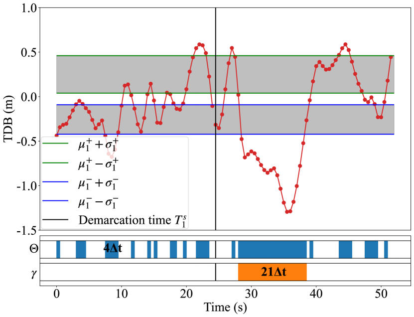
(a) ${TFV}_{1}$

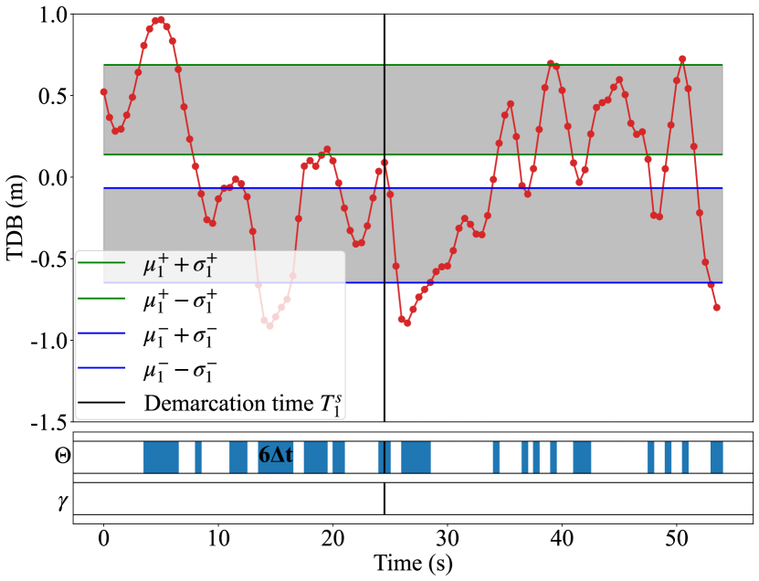
(b) ${FV}_{1}$

Figure 6: The process of quantifying lane-changing impact in a lane-changing instance (vehicle 2783 in the L002_F002_ALL data set) (the status of $\Theta_{i}=0$ or $\Upsilon_{i}=0$ is represented by white regions, while $\Theta_{i}=1$ or $\Upsilon_{i}=1$ is represented by colored regions): (a) depicts the process for ${TFV}_{1}$; (b) depicts the process for ${FV}_{1}$.

Fig. 7 illustrates the estimated affected statuses of ${TFV}_{1}$ and ${FV}_{1}$ during three distinct lane-changing instances, highlighting the varied responses of following vehicles. The colored regions represent $\Upsilon_{i}=1$ (affected status), while white regions indicate $\Upsilon_{i}=0$ (unaffected status). When analyzed alongside the third subfigures of Figs. 6(a) and 6(b), it becomes evident that the initial times when vehicles are affected differ among following vehicles, indicating heterogeneity in their responses. These initial affected times do not necessarily coincide with $T_{1}^{s}$ (the moment when the following vehicle first encounters the deceleration wave), as shown in Fig. 7(a) and the third subfigure of Fig. 6(a). This suggests that the following vehicle may not immediately react to the lane-changing vehicle’s maneuver. This behavior can be attributed to the relaxation phenomena in lane-changing processes, where a lane-changer (or a follower) may initially accept very short spacings before gradually returning to more normal spacings (Laval and Leclercq, 2008; Zheng et al., 2013).

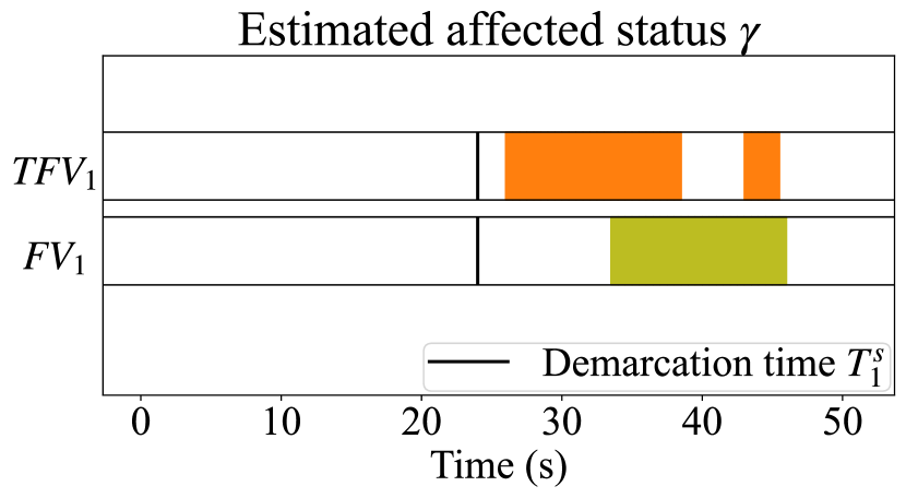
(a)

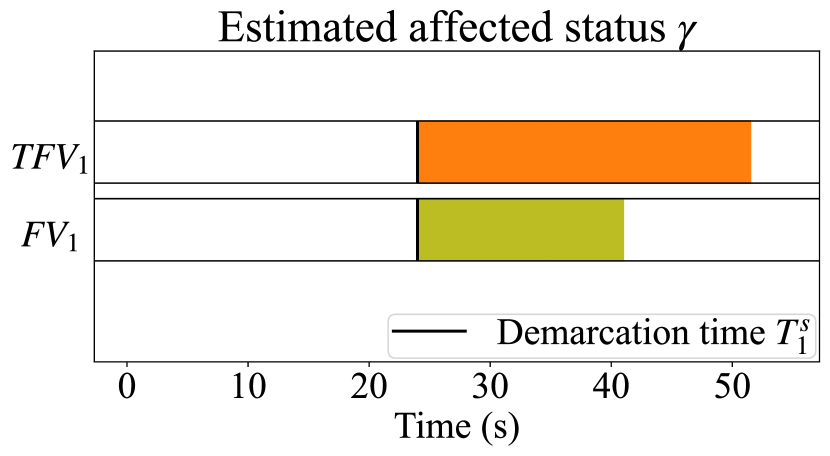
(b)

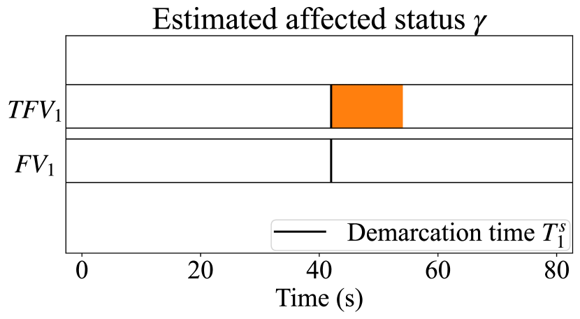
(c)

Figure 7: Estimated affected statuses of ${TFV}_{1}$ and ${FV}_{1}$ in three lane-changing instances (the status of $\Upsilon_{i}=0$ is represented by white regions, while $\Upsilon_{i}=1$ is represented by colored regions): (a) Vehicle 205 in the L001_F002_ALL data set; (b) Vehicle 699 in the L001_F002_ALL data set; and (c) Vehicle 2891 in the L002_F002_ALL data set

Furthermore, Fig. 7(a) reveals that ${TFV}_{1}$ transitions from being affected to unaffected and then back to affected. This pattern suggests that drivers may adjust their acceptable spacing through multiple steps rather than a single adjustment, highlighting the dynamic and complex nature of driver behavior during the lane-changing process. This complexity cannot be fully captured by simplistic models that assume instantaneous and single-step responses. Such discontinuous influence processes are not accounted for in existing methods (Zheng et al., 2013; He et al., 2023), showcasing the superiority of our proposed approach in detecting a more nuanced impact process. Additionally, Fig. 7(c) show that while ${TFV}_{1}$ is affected, ${FV}_{1}$ remains unaffected, indicating that ${FV}_{1}$ does not adjust its spacing in response to the departure of the lane-changing vehicle.

These observations underscore that the following vehicles exhibit varying levels of sensitivity or responsiveness to lane-changing events, potentially influenced by factors such as driver perception, vehicle characteristics, or prevailing traffic conditions.

4.2 Quantitative results

Fig. 8 illustrates the distribution of lane-changing impact duration and magnitude for the first following vehicles on both the target and original lanes. The average impact duration ($T_{i}^{A}$ as defined in Eq. (24)) and magnitude ($w_{i}^{A}$ as defined in Eq. (29)) for ${TFV}_{1}$ were approximately 14.2 seconds and -2.1 meters, respectively. For ${FV}_{1}$, these values were approximately 12.3 seconds and 3.5 meters, respectively. These findings align with existing research (He et al., 2023), supporting the validity of our proposed method for quantifying lane-changing impacts.

Comparing Figs. 8(c) and 8(d), it is evident that lane changes have a more negative impact on the efficiency of the target lane, while they improve efficiency in the original lane. This distinction is not captured by the method proposed by He et al. (2023), which only offers the affected duration or the number of affected vehicles. Our approach demonstrates an advantage by distinguishing between positive and negative influences.

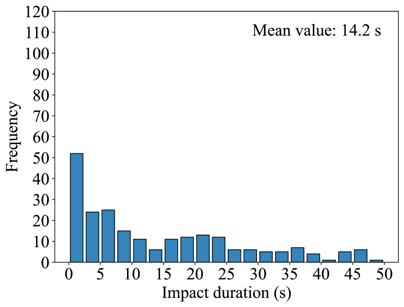
(a) Impact duration for ${TFV}_{1}$

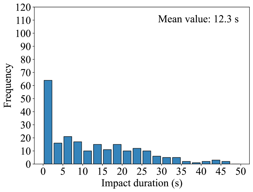
(b) Impact duration for ${FV}_{1}$

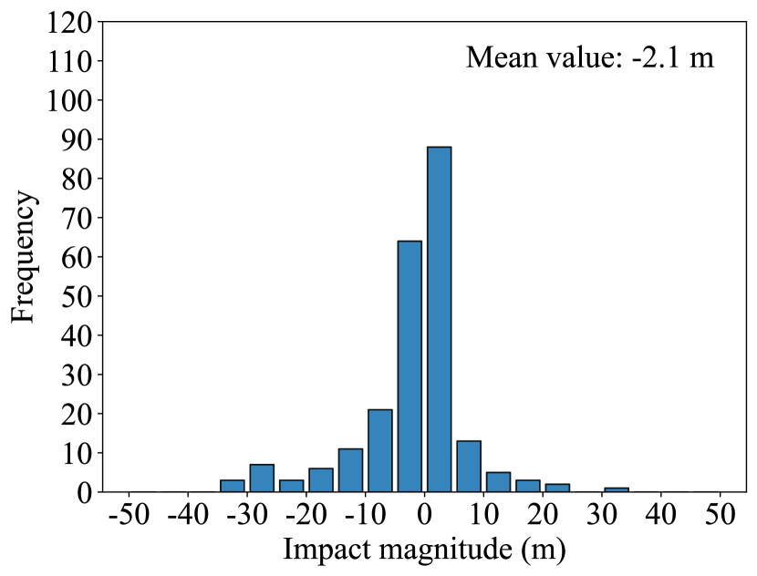
(c) Impact magnitude for ${TFV}_{1}$

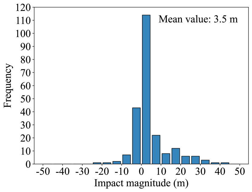
(d) Impact magnitude for ${FV}_{1}$

Figure 8: Distribution of lane-changing impact for the first following vehicles: (a) Impact duration for ${TFV}_{1}$; (b) Impact duration for ${FV}_{1}$; (c) Impact magnitude for ${TFV}_{1}$ and (d) Impact magnitude for ${FV}_{1}$

We further analyze the average overall impact duration (as defined by $T^{A}$ in Eq. (35)), the total number of affected following vehicles (as defined by $N_{A}$ in Eq. (30), and the total cumulative spatiotemporal impact magnitude (as defined by $W^{A}$ in Eq. (31)) caused by a single lane change, as illustrated in Fig. 9. The results show that the average impact durations are 23.8 seconds in the target lane and 25 seconds in the original lane. The total number of affected following vehicles averages 5.6 vehicles in the target lane and 5.3 vehicles in the original lane. The total impact magnitude in terms of CTDB is -10.8 meters in the target lane and 4.7 meters in the original lane.

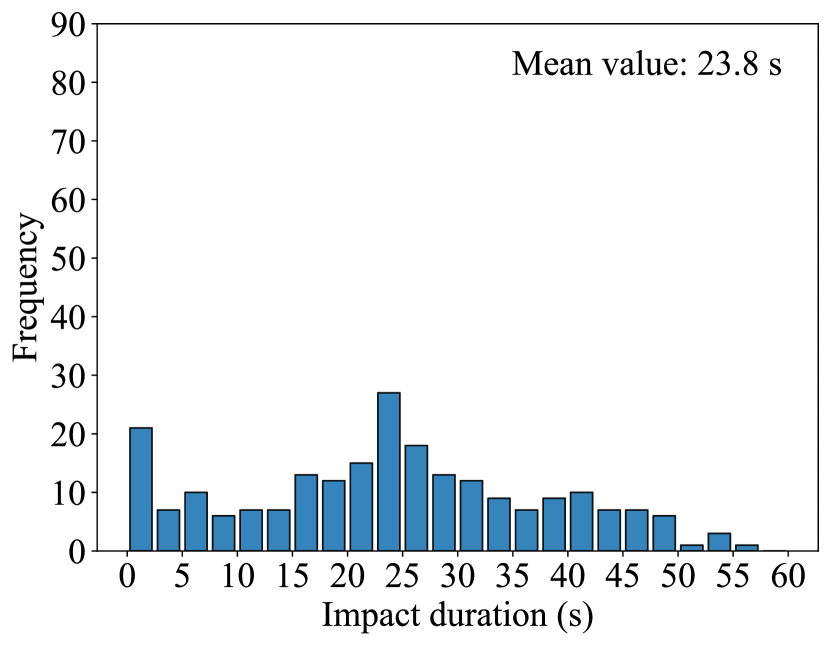
(a) Target lane

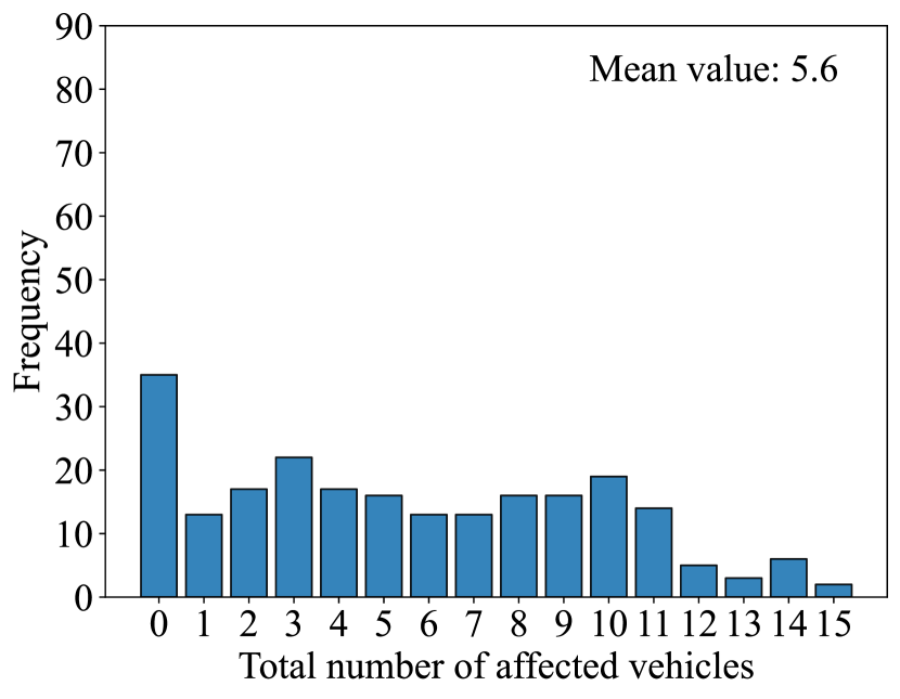
(b) Target lane

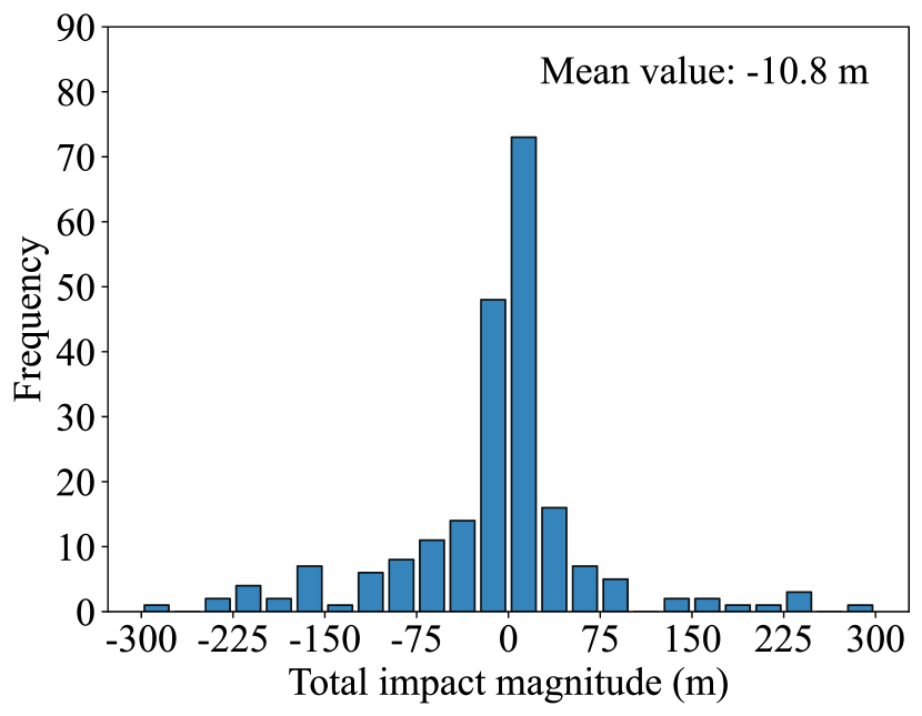
(c) Target lane

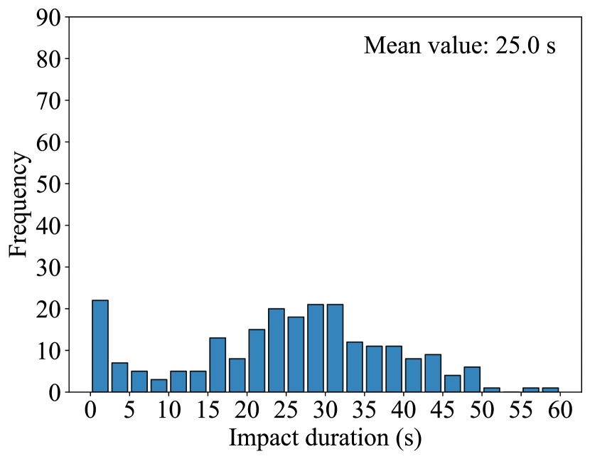
(d) Original lane

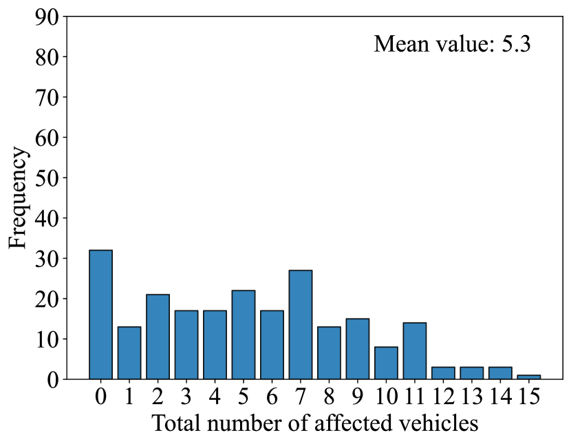
(e) Original lane

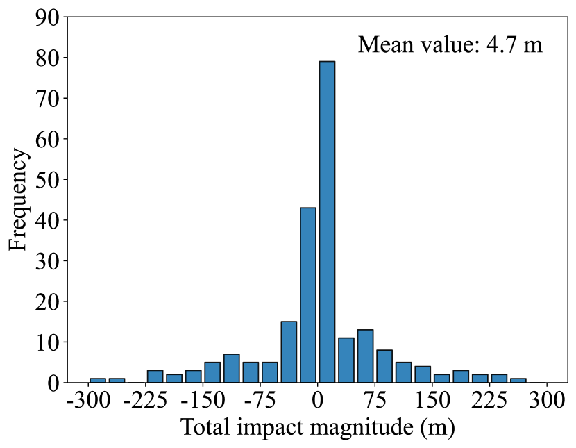
(f) Original lane

Figure 9: Distribution of lane-changing impact duration, total number of affected vehicles and total impact magnitude on different lanes: (a)(b)(c) correspond to the target lane; (d)(e)(f) correspond to the original lane

Considering the joint impact of a single lane change on both the target and original lanes, we analyze the global impact magnitude as depicted in Fig. 10. The results show an average global impact magnitude of -6.1 meters, indicating negative effects of lane-changing on both lanes. However, it is notable that in some instances, the global total impact magnitude is positive. This observation indicates that certain lane-changing behavior contribute positively to the overall traffic flow dynamics, potentially enhancing the efficiency of the traffic system.

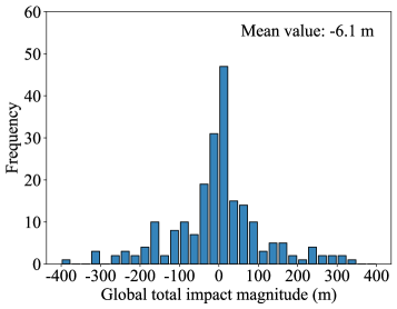
Figure 10: Global total impact magnitude for both the target and original lanes

5 Concluding remarks

In this study, we introduce a comprehensive framework to assess the impact of a single discretionary lane change by analyzing trajectory data characteristics before and after the lane change. Our methodology provides a deterministic assessment of the lane-changing impact on upstream vehicles in both the original and target lanes.

Central to our approach is the introduction of TDB and CTDB. These metrics dynamically account for the fluctuating vehicle speeds due to inherent traffic dynamics, thus providing a more accurate quantification of lane-changing impacts. Notably, the CTDB can differentiate between positive and negative impacts on traffic efficiency. Moreover, it can be integrated with spatiotemporal impact ranges to measure the cumulative impact magnitude, resulting in a more refined and precise quantification.

Given that this paper focuses on the spatiotemporal impact analysis of a single lane change, the extracted data necessitates extensive time periods and large spatial scales, which limits the sample size due to the typically short road length available in open-source datasets. Consequently, the analysis of the magnitude of lane-changing impact cannot be as detailed and comprehensive as desired. With access to more extensive and satisfactory datasets, we would like to further analyze the effects to enhance the robustness and generalizability of our findings.

Nonetheless, this research addresses significant gaps (Table 1) in lane-changing impact studies and facilitates more informed and efficient lane-changing decisions, which is particularly beneficial for automated vehicles aiming for globally optimal decision-making. Future research can expand upon our proposed framework in several promising directions, such as quantifying lane-changing impacts in terms of safety, stability, efficiency (capacity), and fuel consumption, as our framework accurately determines the definitive impact duration for each subsequent vehicle. Additionally, future studies could assist AVs in making lane-changing decisions by considering the spatiotemporal continuity of the lane-changing impact, facilitating optimal decisions. Another avenue could involve quantifying lane-changing impacts in congestion or complex scenarios, such as ramp merging and diverging areas, to aid AVs in making better merging and diverging decisions.

References

- Ali et al. (2022) Ali, Y., Hussain, F., Bliemer, M.C., Zheng, Z., Haque, M.M., 2022. Predicting and explaining lane-changing behaviour using machine learning: A comparative study. Transportation research part C: emerging technologies 145, 103931.
- Ali et al. (2021) Ali, Y., Zheng, Z., Haque, M.M., Yildirimoglu, M., Washington, S., 2021. Clacd: A complete lane-changing decision modeling framework for the connected and traditional environments. Transportation Research Part C: Emerging Technologies 128, 103162.
- Chen et al. (2023a) Chen, K., Knoop, V.L., Liu, P., Li, Z., Wang, Y., 2023a. How gaps are created during anticipation of lane changes. Transportmetrica B: Transport Dynamics 11, 958–978.
- Chen et al. (2023b) Chen, K., Knoop, V.L., Liu, P., Li, Z., Wang, Y., 2023b. Modeling the impact of lane-changing’s anticipation on car-following behavior. Transportation research part C: emerging technologies 150, 104110.
- Chiabaut et al. (2009) Chiabaut, N., Buisson, C., Leclercq, L., 2009. Fundamental diagram estimation through passing rate measurements in congestion. IEEE Transactions on Intelligent Transportation Systems 10, 355–359.
- Coifman et al. (2006) Coifman, B., Mishalani, R., Wang, C., Krishnamurthy, S., 2006. Impact of lane-change maneuvers on congested freeway segment delays: Pilot study. Transportation Research Record 1965, 152–159.
- Dong et al. (2021) Dong, C., Wang, H., Li, Y., Shi, X., Ni, D., Wang, W., 2021. Application of machine learning algorithms in lane-changing model for intelligent vehicles exiting to off-ramp. Transportmetrica A: transport science 17, 124–150.
- Feng et al. (2015) Feng, S., Li, J., Ding, N., Nie, C., 2015. Traffic paradox on a road segment based on a cellular automaton: Impact of lane-changing behavior. Physica A: Statistical Mechanics and its Applications 428, 90–102.
- Gao et al. (2023) Gao, K., Li, X., Chen, B., Hu, L., Liu, J., Du, R., Li, Y., 2023. Dual transformer based prediction for lane change intentions and trajectories in mixed traffic environment. IEEE Transactions on Intelligent Transportation Systems .
- He et al. (2023) He, J., Qu, J., Zhang, J., He, Z., 2023. The impact of a single discretionary lane change on surrounding traffic: An analytic investigation. IEEE Transactions on Intelligent Transportation Systems 24, 554–563.
- Holland (1998) Holland, E., 1998. A generalised stability criterion for motorway traffic. Transportation Research Part B: Methodological 32, 141–154.
- Hou et al. (2024) Hou, K., Zheng, F., Liu, X., Fan, Z., 2024. Cooperative vehicle platoon control considering longitudinal and lane-changing dynamics. Transportmetrica A: Transport Science 20, 2182143.
- Hou et al. (2023) Hou, K., Zheng, F., Liu, X., Guo, G., 2023. Cooperative on-ramp merging control model for mixed traffic on multi-lane freeways. IEEE Transactions on Intelligent Transportation Systems .
- Huang et al. (2024) Huang, T., Fu, R., Sun, Q., Deng, Z., Liu, Z., Jin, L., Khajepour, A., 2024. Driver lane change intention prediction based on topological graph constructed by driver behaviors and traffic context for human-machine co-driving system. Transportation Research Part C: Emerging Technologies 160, 104497.
- Jin (2010) Jin, W.L., 2010. A kinematic wave theory of lane-changing traffic flow. Transportation research part B: methodological 44, 1001–1021.
- Jin (2013) Jin, W.L., 2013. A multi-commodity lighthill–whitham–richards model of lane-changing traffic flow. Transportation Research Part B: Methodological 57, 361–377.
- Kesting et al. (2007) Kesting, A., Treiber, M., Helbing, D., 2007. General lane-changing model mobil for car-following models. Transportation Research Record 1999, 86–94.
- Kodupuganti and Pulugurtha (2023) Kodupuganti, S.R., Pulugurtha, S.S., 2023. Are facilities to support alternative modes effective in reducing congestion?: Modeling the effect of heterogeneous traffic conditions on vehicle delay at intersections. Multimodal Transportation 2, 100050.
- Laval and Leclercq (2008) Laval, J.A., Leclercq, L., 2008. Microscopic modeling of the relaxation phenomenon using a macroscopic lane-changing model. Transportation Research Part B: Methodological 42, 511–522.
- Li et al. (2022) Li, G., Yang, Y., Li, S., Qu, X., Lyu, N., Li, S.E., 2022. Decision making of autonomous vehicles in lane change scenarios: Deep reinforcement learning approaches with risk awareness. Transportation research part C: emerging technologies 134, 103452.
- Li et al. (2020) Li, M., Li, Z., Xu, C., Liu, T., 2020. Short-term prediction of safety and operation impacts of lane changes in oscillations with empirical vehicle trajectories. Accident Analysis & Prevention 135, 105345.
- Li and Sun (2017) Li, X., Sun, J.Q., 2017. Studies of vehicle lane-changing dynamics and its effect on traffic efficiency, safety and environmental impact. Physica A: Statistical Mechanics and its Applications 467, 41–58.
- Liu et al. (2022) Liu, Y., Zhou, B., Wang, X., Li, L., Cheng, S., Chen, Z., Li, G., Zhang, L., 2022. Dynamic lane-changing trajectory planning for autonomous vehicles based on discrete global trajectory. IEEE Transactions on Intelligent Transportation Systems 23, 8513–8527.
- Montanino and Punzo (2015) Montanino, M., Punzo, V., 2015. Trajectory data reconstruction and simulation-based validation against macroscopic traffic patterns. Transportation Research Part B: Methodological 80, 82–106.
- Newell (2002) Newell, G.F., 2002. A simplified car-following theory: a lower order model. Transportation Research Part B: Methodological 36, 195–205.
- Pan et al. (2016) Pan, T., Lam, W.H., Sumalee, A., Zhong, R., 2016. Modeling the impacts of mandatory and discretionary lane-changing maneuvers. Transportation research part C: emerging technologies 68, 403–424.
- Qin et al. (2021) Qin, Y., Wang, H., Ni, D., 2021. Lighthill-whitham-richards model for traffic flow mixed with cooperative adaptive cruise control vehicles. Transportation Science 55, 883–907.
- Shangguan et al. (2022) Shangguan, Q., Fu, T., Wang, J., Fu, L., et al., 2022. A proactive lane-changing risk prediction framework considering driving intention recognition and different lane-changing patterns. Accident Analysis & Prevention 164, 106500.
- Venthuruthiyil and Chunchu (2022) Venthuruthiyil, S.P., Chunchu, M., 2022. Interrupted and uninterrupted lane changes: a microscopic outlook of lane-changing dynamics. Transportmetrica A: transport science 18, 1679–1698.
- Xie et al. (2019) Xie, D.F., Fang, Z.Z., Jia, B., He, Z., 2019. A data-driven lane-changing model based on deep learning. Transportation research part C: emerging technologies 106, 41–60.
- Xing et al. (2020) Xing, Y., Lv, C., Wang, H., Cao, D., Velenis, E., 2020. An ensemble deep learning approach for driver lane change intention inference. Transportation Research Part C: Emerging Technologies 115, 102615.
- Xu et al. (2020) Xu, H., Zhang, Y., Cassandras, C.G., Li, L., Feng, S., 2020. A bi-level cooperative driving strategy allowing lane changes. Transportation research part C: emerging technologies 120, 102773.
- Yang et al. (2019) Yang, M., Wang, X., Quddus, M., 2019. Examining lane change gap acceptance, duration and impact using naturalistic driving data. Transportation research part C: emerging technologies 104, 317–331.
- Zhang et al. (2023) Zhang, Y., Xu, Q., Wang, J., Wu, K., Zheng, Z., Lu, K., 2023. A learning-based discretionary lane-change decision-making model with driving style awareness. IEEE Transactions on Intelligent Transportation Systems 24, 68–78.
- Zheng (2014) Zheng, Z., 2014. Recent developments and research needs in modeling lane changing. Transportation research part B: methodological 60, 16–32.
- Zheng et al. (2013) Zheng, Z., Ahn, S., Chen, D., Laval, J., 2013. The effects of lane-changing on the immediate follower: Anticipation, relaxation, and change in driver characteristics. Transportation research part C: emerging technologies 26, 367–379.
- Zhu et al. (2022) Zhu, J., Tasic, I., Qu, X., 2022. Flow-level coordination of connected and autonomous vehicles in multilane freeway ramp merging areas. Multimodal transportation 1, 100005.
- Zong et al. (2022) Zong, F., He, Z., Zeng, M., Liu, Y., 2022. Dynamic lane changing trajectory planning for cav: A multi-agent model with path preplanning. Transportmetrica B: transport dynamics 10, 266–292.