Multi-Agent Trajectory Prediction with Difficulty-Guided Feature Enhancement Network

Abstract

Trajectory prediction is crucial for autonomous driving as it aims to forecast the future movements of traffic participants. Traditional methods usually perform holistic inference on the trajectories of agents, neglecting the differences in prediction difficulty among agents. This paper proposes a novel Difficulty-Guided Feature Enhancement Network (DGFNet), which leverages the prediction difficulty differences among agents for multi-agent trajectory prediction. Firstly, we employ spatio-temporal feature encoding and interaction to capture rich spatio-temporal features. Secondly, a difficulty-guided decoder is used to control the flow of future trajectories into subsequent modules, obtaining reliable future trajectories. Then, feature interaction and fusion are performed through the future feature interaction module. Finally, the fused agent features are fed into the final predictor to generate the predicted trajectory distributions for multiple participants. Experimental results demonstrate that our DGFNet achieves state-of-the-art performance on the Argoverse 1&2 motion forecasting benchmarks. Ablation studies further validate the effectiveness of each module. Moreover, compared with SOTA methods, our method balances trajectory prediction accuracy and real-time inference speed. The code is available at https://github.com/XinGP/DGFNet.

I Introduction

Trajectory prediction is a crucial component of current autonomous driving systems. Its goal is to infer the future trajectory distribution of agents based on historical information within the scene. In addition to the historical motion information of the agents, various complex factors must be considered, such as lane markings and traffic light constraints in the map, as well as social interactions between agents. These considerations ensure that the future trajectory distribution can accurately reflect the agents’ movement trends, thereby ensuring the proper functioning of the autonomous driving system.

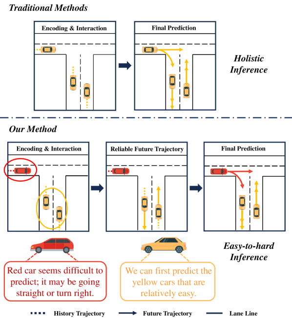
Figure 1: In contrast to traditional trajectory prediction methods, we have incorporated an intermediate step to obtain reliable future trajectories. The lower part of the figure illustrates the varying prediction difficulty among different vehicles in a sample traffic scenario. The future driving trajectory of the yellow vehicle is relatively easy to predict.

Currently, mainstream prediction model architectures can be roughly divided into three steps: feature encoding, feature interaction, and feature decoding. Additionally, some methods improve the accuracy and robustness of prediction models through feature enhancement [1, 2, 3, 4, 5, 6, 7, 8, 9]. These methods involve intermediate modeling of future intentions or trajectories and interact and fuse these with the original encoded features. Although these methods significantly improve model performance compared to mainstream model architectures, they neglect the inherent heterogeneity in prediction difficulty among agents, i.e., the natural differences in prediction difficulty for different agents within the scene. As illustrated in the Fig. 1, The primary difference in our pipeline is the addition of an intermediate module that generates reliable future trajectories, thereby better prediction results can be achieved for agents with higher prediction difficulty.

In real driving scenarios, human drivers often predict the future behaviors of most agents subconsciously, relying on intuition. However, when faced with agents that may pose risks and exhibit high prediction difficulty, human drivers tend to carefully consider their behavior and motivations [10]. Inspired by human drivers, we aim to investigate the effectiveness of prediction methods that follow the principle of easy-to-hard in multi-agent trajectory prediction tasks.

The main contributions of this paper can be summarised as follows:

1) We introduce a novel network architecture that combines the strengths of two scene representations and leverages the differences in prediction difficulty among agents for multi-agent trajectory prediction, thereby improving overall prediction accuracy.

2) Inspired by human drivers, our method follows the principle of easy-to-hard. By initially predicting the easier-to-predict agents and using their reliable future trajectories for feature interaction and fusion, we enhance the prediction results for agents with higher prediction difficulty.

II Related Work

Future Feature Enhancement. Compared to conventional pipelines, methods that enhance features using future information allow networks to incorporate future constraints and interactions. These methods can be broadly categorized into two approaches: intention and future trajectories. TNT [1] and PECNet [2] model vehicle intention as latent variables and generate different prediction trajectories conditioned on vehicle intentions, forming predicted trajectories under certain constraint conditions. GANet [3] and ADAPT [4] integrate and fuse vehicle intentions for future feature enhancement through feature interaction. Similarly, Prophnet [5] and FFINet [6] model intermediate latent variables in the form of trajectories, where the output of intermediate decoders is one or multiple trajectories. It should be noted that the first prediction results of both Prophnet and FFINet are obtained by decoding only the historical trajectory features, which leads to a large error in both first prediction results. Additionally, there is a method that models future trajectories through planner sampling, followed by feature enhancement [8, 9].

Most relevant to our work is M2I [7], which exploits potential game relationships between vehicles. It uses a Relation Predictor and a Marginal Trajectory Predictor to input the future trajectories of the leader in the game relationship as prior information into the Conditional Trajectory Predictor. However, we find that this method is highly dependent on the accuracy of the inferred game relationships and future trajectories. Therefore, we use the more easily extractable prediction difficulty as a basis for personalized classification.

Scene Representation. Broadly, vectorization can be categorized into two types: scene-centric and agent-centric. Since the pioneer of vectorization, Vectornet, was designed for single-agent trajectory prediction tasks, it naturally took the last frame coordinates of the vehicle to be predicted as the scene center, and expressed the trajectories and map vector coordinates of all other agents around the scene center. The benefit of this approach is that it enables the preservation of global relative pose features of various objects in the scene during feature extraction, and facilitates the embedding of some prior information or trajectory anchors [5, 1].

However, due to the demands of multi-agent trajectory prediction tasks, there has been a shift towards agent-centric scene representation methods. Building upon agent-centric approaches, some methods aim to preserve as much information as possible about the mutual spatial relationships of various objects in the scene [11, 12, 13, 14, 15]. To achieve this, they incorporate local pairwise-relative pose features and extract and fuse the relative pose features through networks. However, such methods suffer from the limitation that historical and predicted trajectories only retain local motion characteristics, making it inconvenient to embed anchor and prior information. Therefore, we aim to preserve the advantages of each method by integrating the two approaches.

III Method

III-A Overview

We propose DGFNet, a network designed for multi-agent trajectory prediction using a Difficulty-Guided Feature Enhancement module for asynchronous interaction between historical trajectories and reliable future trajectories. As shown in Fig. 3, the architecture of DGFNet can be divided into three components: spatio-temporal feature encoding, feature interaction, and trajectory decoding.

(1)Spatio-temporal Feature Extraction. This component extracts spatio-temporal features separately from agent-centric historical trajectory information and scene-centric information using both agent-centric and scene-centric approaches. (2)Feature Interaction. The difference with spatio-temporal feature extraction is that the feature extraction component is compatible for both scenarios. However, feature interaction is not. The feature interaction component is categorized into two types: multi-head attention module and multi-head attention module with edge features. The two interaction methods are respectively applicable to scene-centric and agent-centric scenario representations. (3)Trajectory Decoder. This component is divided into a difficulty-guided decoder and a final decoder. The difficulty-guided decoder operates during the intermediate process, while the final decoder outputs the final prediction results.

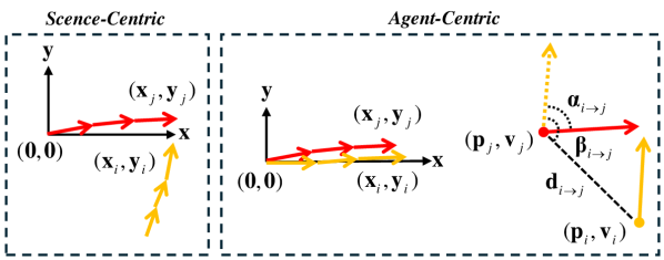
Figure 2: For the same scenario, the left side represents the scene-centric approach, which only requires using coordinate points. On the right side, the agent-centric approach necessitates expressing through local coordinate points and pairwise-relative poses.

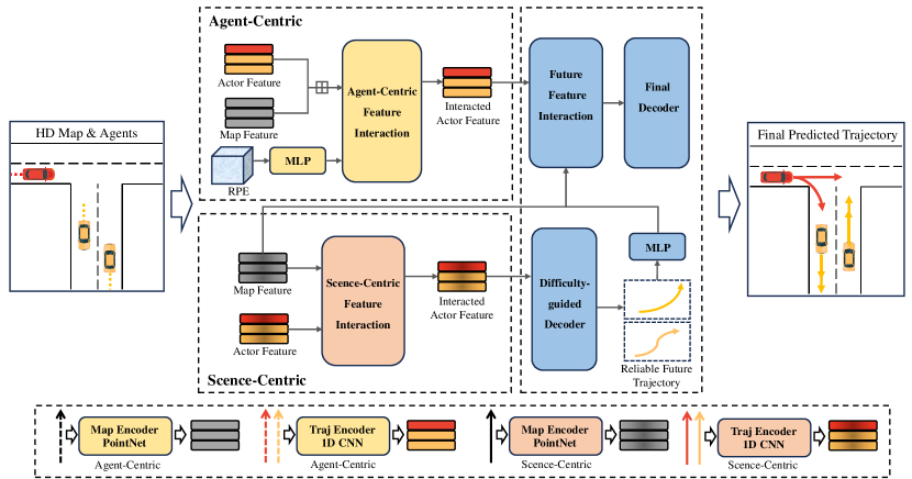
Figure 3: Our spatio-temporal feature extraction includes two sets of independent encoders, which extract features based on scene representations (bottom). Subsequently, the extracted features pass through their respective feature interaction modules to obtain interacted Actor features. Following this, we perform future feature enhancement by interacting reliable future trajectories with Actor and Map features. Finally, these inputs are fed into the final predictor to obtain predicted trajectories and their corresponding probabilities.

III-B Problem formulation

Building on the majority of previous work, such as [16, 17, 1, 13, 18], we assume that upstream perceptual tasks can provide high-quality 2D trajectory tracking data for agents in a coordinate system. At the same time, localisation and mapping tasks can provide accurate self-vehicle positioning data and comprehensive HD map data for the urban environment. In other words, for $j$ agents within a given scene, we obtain $x$ and $y$ positions, denoted as $\mathcal{X}^{0:j}_{-t_{h}:0}$, corresponding to the time stamp horizon $\left\{-t_{h},...,0,1,...,t_{f}\right\}$. The trajectory prediction task consists of predicting the future trajectories $\mathcal{Y}^{0:j}_{1:t_{f}}$ of the agents by using the HD map information $\mathcal{M}$ (including road coordinates, topological links, traffic lights ) within the given scene and the historical trajectories output by the tracking task.

We represent the trajectory information of agents and lane details in vectorized form. To elaborate further, for a given agent $i$ within the scenario, its trajectory information, denoted as $\mathcal{X}^{i}$, is represented as a matrix $\mathcal{X}^{i}_{-t_{h}:0}$ comprising a spatio-temporal sequence$\left\{s^{i}_{-t_{h}},s^{i}_{-t_{h}+1},...,s^{i}_{0}\right\}$ over the past $t_{h}$ time step. Similarly, map information is also segmented into predefined sequence vectors to capture various scene details. Analogous to trajectory vectors, map information is represented as $\mathcal{M}_{1:N}=\left\{s_{1},s_{2},...,s_{N}\right\}$, where $N$ denotes the total vector length. Within each lane vector $s_{i}$, there is an inclusion of lane slice coordinates, lane type (e.g., straight or left-turn lane), and map lane details such as traffic signals. This encapsulates diverse map information pertaining to each lane.

It should be noted that this method involves two types of scenario representations. As shown in Fig. 2, the scene-centric representation involves only one coordinate system, where all agents and lane markings are expressed within this coordinate system. For simplicity, we only use uppercase notation to denote the trajectory and map tensor as $\mathcal{X}$ and $\mathcal{M}$, respectively. In the agent-centric representation, multiple coordinate systems exist. Initially, all agents and lane markings are rotated using matrix rotation so that their orientations align with the x-axis. Subsequently, we use the original coordinates $p$ and velocity orientation $v$ to calculate the relative position distance $d_{i\rightarrow j}$ and the angular difference $\alpha_{i\rightarrow j}$, $\beta_{i\rightarrow j}$. We denote the agent-centric trajectory and map tensor as $\mathcal{A}$ and $\mathcal{L}$, respectively. Pairwise-relative pose is represented as $\mathcal{RPE}=\left\{||d_{i\rightarrow j}||,\sin(\alpha_{i\rightarrow j}),\cos(\alpha_{i\rightarrow j}),\sin(\beta_{i\rightarrow j}),\cos(\beta_{i\rightarrow j})\right\}$.

III-C Spatio-temporal feature extraction

In the problem formulation, we explain the process of representing agent and high-definition (HD) map data as vectors, establishing a corresponding mapping between continuous trajectories, map annotations, and sets of vectors. This vectorization method allows us to encode trajectory and map information as vectors. Following the trajectory feature extraction method of LaneGCN, our trajectory feature extraction module mainly uses 1D CNN and downsampling techniques to encode the historical trajectories of all vehicles in the scene, thus obtaining encoded historical trajectory features. For map tensor, we use the PointNet [19] to encode lane nodes and structural information to obtain map features. It is worth mentioning that when processing scene-centric vector information, we do not mix vehicle historical trajectories and lane line information. Our view is that vehicle trajectories, as dynamic vectors, need to be distinguished from static maps to better capture the local motion characteristics of the vehicles. For the extraction of historical trajectory features are described by this:

$$\mathcal{Z}_{i}=\mathbf{Conv1d}(\mathbf{Res1d}(\mathcal{X}_{i}))\quad\text{for }i=0,1,\dots,n_{\text{fpn}}-1$$ (1)

$$\hat{\mathcal{X}}_{i}=\mathbf{Inter}(\mathcal{Z}_{i+1},\text{scale\_factor}=2)+\mathcal{Z}_{i}$$ (2)

after Res1d and Conv1d encoding, feature alignment is performed by scaling and interpolation operations. For the agent-centric trajectory tensor, the same feature extraction is used to obtain $\hat{\mathcal{A}}$.

For map feature extraction is described by this:

$${\mathcal{H}}_{1} =\mathbf{PAB}_{1}\left(\mathbf{ReLU}(\mathbf{LayerNorm}(\mathcal{M}{W}_{p}+{b}_{p}))\right)$$ (3)

$$\hat{\mathcal{M}} =\mathbf{PAB}_{2}({\mathcal{H}}_{1})$$ (4)

where $\mathcal{M}\in\mathbb{R}^{N_{\text{lane}}\times 10\times C_{\text{in}}}$ are the input lane features, ${W}_{p}\in\mathbb{R}^{C_{\text{in}}\times h}$ and $\mathbf{b}_{p}\in\mathbb{R}^{h}$ are the weights and biases for the projection layer, and PAB represents the PointAggregateBlock.

Similarly, we can obtain the agent-centric map feature $\hat{\mathcal{L}}$. For $\mathcal{RPE}$ we use MLPs for feature extraction to get $\hat{\mathcal{RPE}}$.

III-D Feature interaction

Our intention was to utilize the global representation of scence-centric scenes to embed future trajectory features. Interestingly we found that even without any future enhancement, just concatenating the Actor features after the two interactions gives a better boost. Specific results can be seen later in the ablation experiments. Here we will present the two interaction methods: multi-head attention module and multi-head attention module with edge features, respectively.

We first introduce a generic feature interaction block. In contrast to the general method, which uses simple attention operations for feature interaction, we believe that multi-head attention mechanisms are often better suited to handle complex input sequences and capture a wider range of hierarchical and diverse information. We opt for Multi-Head Attention Blocks (MHAB) instead of the previously used simple attention operations, as used for the features [20].

$$\mathbf{MHA}(Q,K,V)=\mathbf{softmax}\left(\frac{QK^{T}}{\sqrt{dim_{k}}}\right)V$$ (5)

$$Q,K,V=W^{q},W^{k},W^{v}$$ (6)

where $\mathbf{MHA}$ denotes the Multi-Head Attention operation. $Q$, $K$, $V$ are computed by linear projections $W^{q}$, $W^{k}$, $W^{v}$ applied to input vectors. The attention mechanism computes scaled dot-product attention using $Q$ and $K$, and applies it to $V$ after softmax normalization.

The feature interaction module for carrying edge features is described as follows:

$$\mathbf{MHA}(Q^{\prime},K^{\prime},V^{\prime})=\mathbf{softmax}\left(\frac{Q^{\prime}K^{\prime T}}{\sqrt{dim_{k}}}\right)V^{\prime}$$ (7)

$$Q^{\prime},K^{\prime},V^{\prime}=Q+W^{q}\text{edge}^{\prime},K+W^{k}\text{edge}^{\prime},V+W^{v}\text{edge}^{\prime}$$ (8)

here, $Q^{\prime},K^{\prime},V^{\prime}$ are the query, key, and value tensors after linear transformations that incorporate edge features, and $\text{edge}^{\prime}$ is the edge feature after linear transformation.

Finally, the normalized output after attention and dropout application is:

$$\hat{x}=\mathbf{LayerNorm}(x+\mathbf{Drop}(\mathbf{MHA}(Q^{\prime},K^{\prime},V^{\prime})))$$ (9)

For ease of expression, we denote regular multi-head attention as $\mathbf{MHA}$ and multi-head attention with edge features as $\mathbf{MHA}_{edge}$. Our Scene-centric Feature Interaction can be denoted as follows:

$$\hat{\mathcal{X}}^{(l)}=\mathbf{MHA}_{MA}(\hat{\mathcal{M}}^{(l-1)},\hat{\mathcal{X}}^{(l-1)})$$ (10)

$$\hat{\mathcal{M}}^{(l)}=\mathbf{MHA}_{MM}(\hat{\mathcal{M}}^{(l-1)})$$ (11)

$$\hat{\mathcal{M}}^{(l)}=\mathbf{MHA}_{AM}(\hat{\mathcal{X}}^{(l)},\hat{\mathcal{M}}^{(l-1)})$$ (12)

$$\hat{\mathcal{X}}^{(l)}=\mathbf{MHA}_{AA}(\hat{\mathcal{X}}^{(l-1)})$$ (13)

here, $l$ denotes the current layer index, and $\hat{\mathcal{X}}^{(0)}=\hat{\mathcal{X}}$ and $\hat{\mathcal{M}}^{(0)}=\hat{\mathcal{M}}$ are the initial inputs.

Our Agent-centric Feature Interaction can be denoted as follows:

$$\hat{\mathcal{A}}^{(k)}=\mathbf{MHA}_{edge}(\hat{\mathcal{A}}^{(k-1)},\hat{\mathcal{L}}^{(k-1)},\hat{\mathcal{RPE}}^{(k-1)})$$ (14)

similarly we complete multiple rounds of interactions by looping through multiple levels of updates.

III-E Difficulty-guided decoder

To take advantage of the different prediction difficulties of different agents in the scenario, we developed the Difficulty Guided Feature Enhancement Module, which consists of a Difficulty Guided Trajectory Decoder and a Future Feature Interaction Module.

To capture features of plausible future trajectories in the scene, we introduce a Difficulty-Guided Decoder to obtain the future trajectories of agents that are relatively easier to predict. Firstly, we decode the actor features $\hat{\mathcal{X}}^{(l)}$ in scence-centric, which have undergone multiple layers of feature interactions. Each agent receives six predicted trajectories. Following the ADAPT [4] trajectory decoder to get higher quality decoded trajectories by predicting endpoints for refinement. The decoding process can be expressed as follows:

$$\hat{\mathcal{E}}=\mathbf{MLP}_{\text{end}}(\hat{\mathcal{X}}^{(l)})+\mathbf{MLP}_{\text{refine}}(\text{cat}[\hat{\mathcal{X}}^{(l)},\hat{\mathcal{E}}])$$ (15)

$$\hat{\mathcal{P}}=\text{cat}[\mathbf{MLP}_{\text{traj}}(\text{cat}[\hat{\mathcal{X}}^{(l)},\hat{\mathcal{E}}]),\hat{\mathcal{E}}]$$ (16)

where endpoints $\hat{\mathcal{E}}$ are predicted and refined by concatenating with the agent features $\hat{\mathcal{X}}^{(l)}$, then the trajectories $\hat{\mathcal{P}}$ are predicted and merged with the refined endpoints.

Algorithm 1 Difficulty Masker for Predicted Trajectories

0:  Predicted trajectories $\hat{\mathcal{P}}$, Predicted endpoints $\hat{\mathcal{E}}$, threshold $\tau$

0:  Masked trajectories $\hat{\mathcal{P}}_{masked}$

1:  $\hat{\mathcal{P}}_{masked}=set()$

2:  $\bar{\mathcal{E}}\leftarrow\hat{\mathcal{E}}.mean()$

3:  for $i=1$ to $N$ do

4:     $\mathcal{D}=\|\hat{\mathcal{E}}-\bar{\mathcal{E}}\|_{2}$

5:     $\bar{\mathcal{D}}\leftarrow\mathcal{D}.mean()$

6:     if $\bar{\mathcal{D}}\leq\tau$ then

7:        $\hat{\mathcal{P}}_{masked}$.add($\hat{\mathcal{P}}_{l}$)

8:  

9:  return  $\hat{\mathcal{P}}_{masked}$

The Argoverse 1 dataset show that the predicted trajectories of most of the vehicles in the scenarios exhibit a high degree of concentration, with more than 90% of the samples of straight ahead trajectories in each case [21]. This suggests that the motion patterns of most agents can be easily captured, reflecting real-world traffic scenarios. In order to prevent higher difficulty prediction trajectories from entering the subsequent modules and generating cumulative errors, we introduced a difficulty masker to filter the initial prediction results. ScenceTransformer[22], inspired by recent approaches to language modeling, has pioneered the idea of using a masking strategy as a query to the model, enabling it to invoke a single model to predict agent behavior in multiple ways (marginal or joint prediction). This mechanism in this paper is intended to mask out the initial prediction trajectories of the more difficult agents, thus providing better control over the prediction accuracy. This process can be formalized as Algo. 1.

III-F Future feature enhancement

For the reliable future trajectories we first flatten them by performing the flatten operation on multiple future trajectories for feature dimension alignment. Then future trajectory feature extraction is performed by a simple MLP layer. These two operations can be formulated as:

$$\hat{\mathcal{F}}=\mathbf{MLP}(\mathbf{flatten}(\hat{\mathcal{P}}_{\text{masked}}))$$ (17)

Subsequently, we interact the future trajectory feature $\hat{F}$ with the agent-centric interactive actor feature $\hat{\mathcal{A}}^{(k)}$ via multi-head attention. This operation aims to impose certain constraints on the prediction of other agents through the reliable future trajectory features. Finally, we need to perform one last interaction using the original map features $\hat{\mathcal{M}}$. This step is crucial as it aims to refocus on the reachable lane lines of the map after imposing social constraints through the future trajectory features[23]. These two operations can be formulated as:

$$\mathcal{H}=\mathbf{MHA}_{AF}(\hat{\mathcal{A}}^{(k)},\hat{\mathcal{F}})$$ (18)

$$\hat{\mathcal{O}}=\mathbf{MHA}_{AM}(\mathcal{H},\hat{M})$$ (19)

III-G Final prediction

We perform feature fusion operations on the final features $\hat{O}$ and the scence-centric feature $\hat{X}^{(l)}$, expanding the decoding dimension to 256. Our final predictor can generate multimodal trajectories for all agents in the scene and their corresponding probabilities in a single inference. This process can be described as follows:

$${\mathcal{A}}_{fusion}=\text{cat}(\hat{\mathcal{O}},\hat{\mathcal{X}}^{(l)})$$ (20)

$$\mathcal{E}=\mathbf{MLP}_{\text{end}}({\mathcal{A}}_{fusion})+\mathbf{MLP}_{\text{refine}}(\text{cat}[{\mathcal{A}}_{fusion},\mathcal{E}])$$ (21)

$$\mathcal{K}=\mathbf{softmax}(\mathbf{MLP}_{\text{cls}}(\text{cat}[\mathcal{A}_{fusion},\mathcal{E}]))$$ (22)

$$\mathcal{P}=\text{cat}[\mathbf{MLP}_{\text{traj}}(\text{cat}[{\mathcal{A}}_{fusion},\mathcal{E}]),\mathcal{E}]$$ (23)

here, $\mathcal{P}$ represents the multimodal prediction trajectory and its corresponding probability $\mathcal{K}$ that we finally obtain.

Table I: Comparisons with the state-of-the-art methods listed on the leaderboard of the Argoverse 1 motion Forecasting test set. The numbers highlighted in bold represent the best-performing results among them.

Inference	Methods	Year	p-minFDE $\downarrow$	minFDE $\downarrow$	MR $\downarrow$	minADE $\downarrow$	minFDE $\downarrow$	minADE $\downarrow$	DAC $\uparrow$
			(K=6)	(K=6)	(K=6)	(K=6)	(K=1)	(K=1)
Single model	LaneGCN [16]	2020	2.05	1.36	0.162	0.87	3.76	1.70	0.9812
	THOMAS [24]	2021	1.97	1.44	0.104	0.94	3.59	1.67	0.9781
	HiVT-128 [13]	2022	1.84	1.17	0.127	0.77	3.53	1.60	0.9888
	LAformer [25]	2023	1.84	1.16	0.125	0.77	3.45	1.55	0.9897
	HeteroGCN [26]	2023	1.84	1.19	0.120	0.82	3.52	1.62	-
	Macformer [27]	2023	1.83	1.22	0.120	0.82	3.72	1.70	0.9906
	GANet [3]	2023	1.79	1.16	0.118	0.81	3.46	1.59	0.9899
	DGFNet(single model)	-	1.74	1.11	0.108	0.77	3.34	1.53	0.9909
Ensembled model	HOME+GOHOME [28, 29]	2022	1.86	1.29	0.085	0.89	3.68	1.70	0.9830
	HeteroGCN-E [26]	2023	1.75	1.16	0.117	0.79	3.41	1.57	0.9886
	Macformer-E [27]	2023	1.77	1.21	0.127	0.81	3.61	1.66	0.9863
	Wayformer [30]	2023	1.74	1.16	0.119	0.77	3.66	1.64	0.9893
	ProphNet [5]	2023	1.69	1.13	0.110	0.76	3.26	1.49	0.9893
	QCNet [31]	2023	1.69	1.07	0.106	0.73	3.34	1.52	0.9887
	FFINet [6]	2024	1.73	1.12	0.113	0.76	3.36	1.53	0.9875
	DGFNet(ensembled model)	-	1.69	1.11	0.107	0.75	3.36	1.53	0.9902

Model Training. Although our feature enhancement component outputs trajectories during the intermediate process, our training process remains end-to-end. Our DGFNet obtains initial and final predictions in a single pass. Similar to the previous method [16, 17, 1, 13], we supervise the output trajectories $P$ and $\hat{\mathcal{P}}$ during the training process by smoothing the $\mathcal{L}1$ loss, which is expressed as ${\mathcal{L}}_{reg}$ and ${\mathcal{L}}_{reg}^{c}$. For the categorization loss in $\mathcal{K}$, we use the maximum marginal loss, which is expressed as ${\mathcal{L}}_{cls}$. Our overall loss expression is as follows:

$$\mathcal{L}=\alpha{\mathcal{L}}_{reg}+\beta{\mathcal{L}}_{cls}+\lambda{\mathcal{L}}_{reg}^{c}$$ (24)

where $\alpha$, $\beta$ and $\lambda$ are three constant weights.

IV Experiments

IV-A Experimental setup

Datasets. Our model DGFNet is tested and evaluated on a very challenging and widely used self-driving motion prediction dataset: the Argoverse 1&2 [32, 33]. Both motion prediction datasets provide agent tracking trajectories and semantically rich map information at a frequency of 10Hz over a specified time interval. The prediction task in Argoverse 1 is to predict trajectories for the next 3 seconds based on the previous 2 seconds of historical data. The dataset contains a total of 324,557 vehicle trajectories of interest extracted from over 1000 hours of driving. Argoverse 2 contains 250,000 of the most challenging scenarios officially filtered from the self-driving test fleet. Argoverse 2 predicts the next 6 seconds from the first 5 seconds of historical trajectory data. To ensure fair comparisons between models, both datasets were subjected to official data partitioning and the test set was evaluated using the Eval online test server.

Evaluation Metrics. We have adopted the standard testing and evaluation methodology used in motion prediction competitions to assess prediction performance. Key metrics for individual agents include Probabilistic minimum Final Displacement Error (p-minFDE), Minimum Final Displacement Error (minFDE), Minimum Average Displacement Error (minADE), Miss Rate (MR) and Drivable Area Compliance (DAC). Where p-minFDE, MR, and minFDE reflect the accuracy of the predicted endpoints, and minADE indicates the overall bias in the predicted trajectories. DAC, reflects the compliance of the predicted outcomes.

Implementation Details. We generate lane vectors for lanes that are more than 50 meters away from any available agent. The number of layers $l$ and $k$ of interaction features are set to 3. All layers except the final decoder have 128 output feature channels. In addition, the weight parameters in the loss function are set to $\alpha$=0.7, $\beta$=0.1 and $\lambda$=0.2. The hyperparameter $\tau$ in the difficulty masker was set to 5. The model was trained 50 epochs on an Nvidia RTX 3090 with a batch size of 16. For the experiments on Argoverse 1&2, we used a segmented constant learning rate strategy: up to the 5th epoch we used $5\times 10^{-5}$; from the 6th epoch to the 40th, we used $5\times 10^{-4}$; and thereafter, we used $5\times 10^{-5}$ until training was complete.

IV-B Quantitative Results

Quantitative evaluations on the Argoverse 1&2 datasets demonstrate that DGFNet exhibits significant performance advantages across various metrics compared to state-of-the-art methods. Our method remains competitive even when compared to ensemble strategies used by other top models like QCNet and ProphNet. Through an ablation study, we validate the effectiveness of scene feature fusion, future feature interaction, and a difficulty masking mechanism, resulting in substantial improvements in prediction accuracy. Computational efficiency analysis shows that DGFNet achieves high prediction accuracy with relatively fewer parameters, ensuring its practical applicability in real-time autonomous driving scenarios.

Comparison with State-of-the-Arts in Agoverse 1. We conducted performance comparisons on the Argoverse 1 test set using both single-model and multi-model approaches between our method and the most classical and latest state-of-the-art methods. Generally, ensemble methods involve using K-means to match the closest trajectories from multiple models, followed by weighted computation to obtain the final result. We obtained 5 models by setting different initial random seeds and performed ensemble inference using the aforementioned method. The results are shown in Tab.I. Compared to single-model methods, our approach consistently ranks at the top in almost all metrics. Even when compared with methods using ensemble strategies, our approach remains highly competitive, achieving prediction accuracy comparable to the leading models such as QCNet and ProphNet in the leaderboard. However, our method has advantages in terms of parameter size and inference time, which will be detailed in the following sections.

Table II: Comparisons with the state-of-the-art methods listed on the leaderboard of the Argoverse 2 single agent Forecasting.

Method	Year	p-minFDE $\downarrow$	minADE $\downarrow$	minFDE $\downarrow$	MR $\downarrow$
		(K=6)	(K=6)	(K=6)	(K=6)
LaneGCN[16]	2020	2.64	0.91	1.96	0.30
THOMAS[24]	2021	2.16	0.88	1.51	0.20
HDGT[11]	2023	2.24	0.84	1.60	0.21
HPTR[14]	2023	2.03	0.73	1.43	0.19
GoReal[12]	2022	2.01	0.76	1.48	0.22
GANet[3]	2023	1.96	0.72	1.34	0.17
DGFNet	-	1.94	0.70	1.35	0.17

Comparison with State-of-the-Arts in Agoverse 2. In our comparison of performance with several recent single-model inference methods on the Argoverse 2 test set, we found that while the advantage of our method is not as pronounced as in Argoverse 1, it remains reasonably acceptable. We speculate that this is primarily due to the increased prediction horizon in the Argoverse 2 dataset, which has led to less robust initial prediction results. Moreover, due to the inclusion of categories such as pedestrians and cyclists in Argoverse 2, the effectiveness of the parameter settings for our difficulty masker has also been impacted. Overall, our model demonstrates highly competitive performance within an acceptable range of model parameters across both datasets.

Table III: Comparison of prediction performance (minFDE) on high-difficulty samples in the Argoverse 1 validation set.

Method	Top 1%	Top 2%	Top 3%	Top 4%	Top 5%	ALL
LaneGCN	11.52	8.24	6.98	6.67	5.65	1.08
Our base	9.12↓21%	6.86↓17%	5.74↓18%	5.05↓24%	4.57↓19%	0.94↓13%
DGFNet	7.26↓37%	5.21↓36%	4.36↓37%	3.85↓42%	3.51↓30%	0.89↓17%

Comparison of Prediction Performance on High-difficulty Samples. Tab.III shows the highest minFDE errors of each method on the Argoverse 1 validation set. We reasoned on the validation set with LaneGCN’s pre-trained model to obtain some sample sets with the highest errors, and then reasoned on these sample sets using our base model and DGFNet, respectively. It can be observed that the average accuracy difference for all samples is minimal compared to Our base. However, our method, DGFNet, has significantly lower minFDE errors across all percentage ranges, clearly demonstrating the remarkable advantage of our method in mitigating the long-tail problem in trajectory prediction.

Quantitative Results and Visualization. Fig.4 shows the qualitative visualization. The four selected scenarios have high prediction difficulty and strong representativeness. In Seq.1 and Seq.2, the model generates accurate predictions for each agent in a busy and strongly interacting intersection scenario. In Seq.3, the model gives robust predictions in the face of vehicle turning tendencies. As a comparison, in Seq.4 the model gives more scattered prediction results when the intention of the vehicle is not clear. Overall, the model captured the final landing point very accurately in both turning and straight ahead situations.

Table IV: The ablation study results of different components on the Argoverse 1 validation set.

DM	FFI	SFF	p-minFDE $\downarrow$	minADE $\downarrow$	minFDE $\downarrow$
			(K=6)	(K=6)	(K=6)
$\times$	$\times$	$\times$	1.559	0.657	0.941
$\times$	$\times$	✓	1.525	0.646	0.916
$\times$	✓	✓	1.654	0.706	1.052
✓	✓	✓	1.492	0.632	0.892

Table V: Performance versus $\tau$ parameter of DGFNet evaluated on the Argoverse 1 validation set.

$\tau$	p-minFDE $\downarrow$	minADE $\downarrow$	minFDE $\downarrow$
	(K=6)	(K=6)	(K=6)
7	1.510	0.642	0.907
5	1.492	0.632	0.892
3	1.499	0.634	0.897
1	1.508	0.639	0.905

IV-C Analysis and Discussion

Ablation Study. We conducted an ablation study on the Argoverse 1 validation set. The initial model only used agent-centric historical trajectories and maps for feature extraction. The second model incorporated scene-centric features into the initial model, achieving some performance improvement through Scene Feature Fusion (SFF). The third model added the Future Feature Interaction (FFI) module, enabling interaction between extracted historical features and future features. The final model used the Difficulty Masker (DM) to mask out future trajectories that are difficult to predict, ensuring that only reliable trajectories are used for future interaction. Of concern is that without adding Difficulty Masker, the performance of direct future enhancement drops dramatically, failing because the second stage model may find shortcuts during optimization if the results given in the first stage are good enough [34]. According to Tab.IV, comparing the base model with DGFNet, the improvement in predictive performance is evident. And we also did ablation experiments on the effect of parameter $\tau$ on the model. According to Tab.V, the model performance obtained by setting parameter $\tau$ to 5 is the best.

Table VI: Comparison on Computational performance with other methods.

Method	p-minFDE $\downarrow$	Param(M) $\downarrow$	Infer time(ms) $\downarrow$
	(K=6)
LaneGCN[16]	2.054	3.68	17.2
GANet[3]	1.789	5.21	25.3
QCNet* [31]	1.693	7.30	-
HiVT-128[13]	1.842	2.47	13.2
LAformer[25]	1.835	2.59	42.5
FFINet*[6]	1.729	6.20	-
Prophnet*[5]	1.694	15.20	-
DGFNet	1.693	4.53	32.1

Computational Performance. We compared the parameters of each method and the average inference time per scenario on the same device. As shown in Tab.VI, our inference time is slightly higher than LaneGCN and close to the lighter models HiVT-128 and LAformer. However, our method has a much higher prediction accuracy than these two methods. Compared with the methods with the highest prediction accuracy, our method has fewer parameters (note that those marked with * use ensemble strategies), which means that our model achieves high prediction accuracy with lower computational cost. Then, we recorded the inference time on the same experimental machine equipped with an NVIDIA GeForce RTX 3090. The model inference time indicates that the real-time latency of DGFNet is within an acceptable range. Since LAformer uses a two-stage inference approach, its inference time is longer despite having fewer parameters than our method.

V Conclusion

In this paper, we propose a novel Difficulty-Guided Feature Enhancement Network (DGFNet) for muti-agent trajectory prediction. Distinguishing from general future enhancement networks, our model emphasizes filtering future trajectories by masking out and retaining only reliable future trajectories for feature enhancement, which greatly improves the prediction performance. Extensive experiments on the Argoverse 1&2 benchmarks show that our method outperforms most state-of-the-art methods in terms of prediction accuracy and real-time processing. Emulating the predictive habits of human drivers is an intriguing direction for future research. This involves emulating human strategies when encountering different vehicles and making effective assumptions in the presence of incomplete perceptual information.

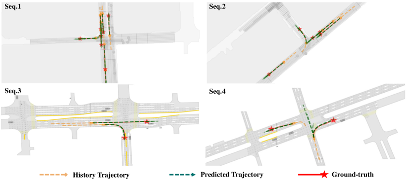
Figure 4: Quantitative results of DGFNet on the Argoverse 1&2 validation set. The top scenarios correspond to the Argoverse 1 dataset and the bottom scenarios correspond to the Argoverse 2 dataset.

References

- [1] H. Zhao, J. Gao, T. Lan, C. Sun, B. Sapp, B. Varadarajan, Y. Shen, Y. Shen, Y. Chai, C. Schmid, et al., “Tnt: Target-driven trajectory prediction,” in Conference on Robot Learning. PMLR, 2021, pp. 895–904.
- [2] K. Mangalam, H. Girase, S. Agarwal, K.-H. Lee, E. Adeli, J. Malik, and A. Gaidon, “It is not the journey but the destination: Endpoint conditioned trajectory prediction,” in Computer Vision–ECCV 2020: 16th European Conference, Glasgow, UK, August 23–28, 2020, Proceedings, Part II 16. Springer, 2020, pp. 759–776.
- [3] M. Wang, X. Zhu, C. Yu, W. Li, Y. Ma, R. Jin, X. Ren, D. Ren, M. Wang, and W. Yang, “Ganet: Goal area network for motion forecasting,” in 2023 IEEE International Conference on Robotics and Automation (ICRA). IEEE, 2023, pp. 1609–1615.
- [4] G. Aydemir, A. K. Akan, and F. Güney, “Adapt: Efficient multi-agent trajectory prediction with adaptation,” in Proceedings of the IEEE/CVF International Conference on Computer Vision, 2023, pp. 8295–8305.
- [5] X. Wang, T. Su, F. Da, and X. Yang, “Prophnet: Efficient agent-centric motion forecasting with anchor-informed proposals,” in Proceedings of the IEEE/CVF Conference on Computer Vision and Pattern Recognition, 2023, pp. 21 995–22 003.
- [6] M. Kang, S. Wang, S. Zhou, K. Ye, J. Jiang, and N. Zheng, “Ffinet: Future feedback interaction network for motion forecasting,” IEEE Transactions on Intelligent Transportation Systems, 2024.
- [7] Q. Sun, X. Huang, J. Gu, B. C. Williams, and H. Zhao, “M2i: From factored marginal trajectory prediction to interactive prediction,” in Proceedings of the IEEE/CVF Conference on Computer Vision and Pattern Recognition, 2022, pp. 6543–6552.
- [8] H. Song, D. Luan, W. Ding, M. Y. Wang, and Q. Chen, “Learning to predict vehicle trajectories with model-based planning,” in Conference on Robot Learning. PMLR, 2022, pp. 1035–1045.
- [9] J. Schmidt, P. Huissel, J. Wiederer, J. Jordan, V. Belagiannis, and K. Dietmayer, “Reset: Revisiting trajectory sets for conditional behavior prediction,” in 2023 IEEE Intelligent Vehicles Symposium (IV). IEEE, 2023, pp. 1–8.
- [10] A. Gulati, S. Soni, and S. Rao, “Interleaving fast and slow decision making,” in 2021 IEEE International Conference on Robotics and Automation (ICRA). IEEE, 2021, pp. 1535–1541.
- [11] X. Jia, P. Wu, L. Chen, Y. Liu, H. Li, and J. Yan, “Hdgt: Heterogeneous driving graph transformer for multi-agent trajectory prediction via scene encoding,” IEEE transactions on pattern analysis and machine intelligence, 2023.
- [12] A. Cui, S. Casas, K. Wong, S. Suo, and R. Urtasun, “Gorela: Go relative for viewpoint-invariant motion forecasting,” in 2023 IEEE International Conference on Robotics and Automation (ICRA). IEEE, 2023, pp. 7801–7807.
- [13] Z. Zhou, L. Ye, J. Wang, K. Wu, and K. Lu, “Hivt: Hierarchical vector transformer for multi-agent motion prediction,” in Proceedings of the IEEE/CVF Conference on Computer Vision and Pattern Recognition, 2022, pp. 8823–8833.
- [14] Z. Zhang, A. Liniger, C. Sakaridis, F. Yu, and L. V. Gool, “Real-time motion prediction via heterogeneous polyline transformer with relative pose encoding,” Advances in Neural Information Processing Systems, vol. 36, 2024.
- [15] L. Zhang, P. Li, S. Liu, and S. Shen, “Simpl: A simple and efficient multi-agent motion prediction baseline for autonomous driving,” IEEE Robotics and Automation Letters, 2024.
- [16] M. Liang, B. Yang, R. Hu, Y. Chen, R. Liao, S. Feng, and R. Urtasun, “Learning lane graph representations for motion forecasting,” in Computer Vision–ECCV 2020: 16th European Conference, Glasgow, UK, August 23–28, 2020, Proceedings, Part II 16. Springer, 2020, pp. 541–556.
- [17] J. Gao, C. Sun, H. Zhao, Y. Shen, D. Anguelov, C. Li, and C. Schmid, “Vectornet: Encoding hd maps and agent dynamics from vectorized representation,” in Proceedings of the IEEE/CVF Conference on Computer Vision and Pattern Recognition, 2020, pp. 11 525–11 533.
- [18] W. Schwarting, A. Pierson, J. Alonso-Mora, S. Karaman, and D. Rus, “Social behavior for autonomous vehicles,” Proceedings of the National Academy of Sciences, vol. 116, no. 50, pp. 24 972–24 978, 2019.
- [19] C. R. Qi, H. Su, K. Mo, and L. J. Guibas, “Pointnet: Deep learning on point sets for 3d classification and segmentation,” in Proceedings of the IEEE conference on computer vision and pattern recognition, 2017, pp. 652–660.
- [20] R. Girgis, F. Golemo, F. Codevilla, M. Weiss, J. A. D’Souza, S. E. Kahou, F. Heide, and C. Pal, “Latent variable sequential set transformers for joint multi-agent motion prediction,” arXiv preprint arXiv:2104.00563, 2021.
- [21] S. Kim, H. Jeon, J. W. Choi, and D. Kum, “Diverse multiple trajectory prediction using a two-stage prediction network trained with lane loss,” IEEE Robotics and Automation Letters, vol. 8, no. 4, pp. 2038–2045, 2022.
- [22] J. Ngiam, B. Caine, V. Vasudevan, Z. Zhang, H.-T. L. Chiang, J. Ling, R. Roelofs, A. Bewley, C. Liu, A. Venugopal, et al., “Scene transformer: A unified architecture for predicting multiple agent trajectories,” arXiv preprint arXiv:2106.08417, 2021.
- [23] Y. Dong, H. Yuan, H. Liu, W. Jing, F. Li, H. Liu, and B. Fan, “Proin: Learning to predict trajectory based on progressive interactions for autonomous driving,” arXiv preprint arXiv:2403.16374, 2024.
- [24] T. Gilles, S. Sabatini, D. Tsishkou, B. Stanciulescu, and F. Moutarde, “Thomas: Trajectory heatmap output with learned multi-agent sampling,” arXiv preprint arXiv:2110.06607, 2021.
- [25] M. Liu, H. Cheng, L. Chen, H. Broszio, J. Li, R. Zhao, M. Sester, and M. Y. Yang, “Laformer: Trajectory prediction for autonomous driving with lane-aware scene constraints,” in Proceedings of the IEEE/CVF Conference on Computer Vision and Pattern Recognition, 2024, pp. 2039–2049.
- [26] X. Gao, X. Jia, Y. Li, and H. Xiong, “Dynamic scenario representation learning for motion forecasting with heterogeneous graph convolutional recurrent networks,” IEEE Robotics and Automation Letters, vol. 8, no. 5, pp. 2946–2953, 2023.
- [27] C. Feng, H. Zhou, H. Lin, Z. Zhang, Z. Xu, C. Zhang, B. Zhou, and S. Shen, “Macformer: Map-agent coupled transformer for real-time and robust trajectory prediction,” IEEE Robotics and Automation Letters, 2023.
- [28] T. Gilles, S. Sabatini, D. Tsishkou, B. Stanciulescu, and F. Moutarde, “Home: Heatmap output for future motion estimation,” in 2021 IEEE International Intelligent Transportation Systems Conference (ITSC). IEEE, 2021, pp. 500–507.
- [29] ——, “Gohome: Graph-oriented heatmap output for future motion estimation,” in 2022 international conference on robotics and automation (ICRA). IEEE, 2022, pp. 9107–9114.
- [30] N. Nayakanti, R. Al-Rfou, A. Zhou, K. Goel, K. S. Refaat, and B. Sapp, “Wayformer: Motion forecasting via simple & efficient attention networks,” in 2023 IEEE International Conference on Robotics and Automation (ICRA). IEEE, 2023, pp. 2980–2987.
- [31] Z. Zhou, J. Wang, Y.-H. Li, and Y.-K. Huang, “Query-centric trajectory prediction,” in Proceedings of the IEEE/CVF Conference on Computer Vision and Pattern Recognition, 2023, pp. 17 863–17 873.
- [32] M.-F. Chang, J. Lambert, P. Sangkloy, J. Singh, S. Bak, A. Hartnett, D. Wang, P. Carr, S. Lucey, D. Ramanan, et al., “Argoverse: 3d tracking and forecasting with rich maps,” in Proceedings of the IEEE/CVF conference on computer vision and pattern recognition, 2019, pp. 8748–8757.
- [33] B. Wilson, W. Qi, T. Agarwal, J. Lambert, J. Singh, S. Khandelwal, B. Pan, R. Kumar, A. Hartnett, J. K. Pontes, et al., “Argoverse 2: Next generation datasets for self-driving perception and forecasting,” arXiv preprint arXiv:2301.00493, 2023.
- [34] R. Geirhos, J.-H. Jacobsen, C. Michaelis, R. Zemel, W. Brendel, M. Bethge, and F. A. Wichmann, “Shortcut learning in deep neural networks,” Nature Machine Intelligence, vol. 2, no. 11, pp. 665–673, 2020.