Optimal closed-loop control of active particles and a minimal information engine

Abstract

To establish general principles of optimal control of active matter, we study the elementary problem of moving an active particle by a trap with minimum work input. We show analytically that (open-loop) optimal protocols are not affected by activity, but work fluctuations are always increased. For closed-loop protocols, which rely on initial measurements of the self-propulsion, the average work has a minimum for a finite persistence time. Using these insights, we derive an optimal cyclic active information engine, which is found to have a higher precision and information efficiency when operated with a run-and-tumble particle than for an active Ornstein-Uhlenbeck particle and, we argue, than for any other type of active particle.

Exploring strategies to control the individual or collective motion of self-propelled particles Schneider and Stark (2019); Falk et al. (2021); Liebchen and Löwen (2019); Baldovin et al. (2023); Shankar et al. (2022) enhances our understanding of active dynamics and represents a first step towards technological applications; ranging from the design of active metamaterials to the construction of nanosized robots. Recent research has explored various means of control, e.g. adjusting the potential landscape Davis et al. (2024); Gupta et al. (2023); Aurell et al. (2011); Ekeh et al. (2020); Majumdar et al. (2022); Blaber and Sivak (2023); Lee et al. (2023), the confinement Malgaretti and Stark (2022); Cocconi et al. (2023), or the level of intrinsic activity Falk et al. (2021). In the realm of small-scale organisms and synthetic machines, high frictional losses and the prevalence of thermal and non-thermal fluctuations become particularly important challenges. In this context, “thermodynamically optimized” control schemes aim to minimize the associated heat dissipation, the work input, or the generated entropy, while transitioning a system from one state to another. Even for passive systems, thermodynamically optimal control can give rise to non-intuitive solutions such as discontinuously time-dependent driving Schmiedl and Seifert (2007); Engel et al. (2023); Whitelam (2023); Loos et al. (2024). To explore the basic principles of thermodynamically optimized control of active systems, which are characterized by noise, memory, (non-)Gaussian statistics and intrinsic driving, it is thus vital to study simplified paradigmatic toy models.

In this spirit, we investigate the elementary problem of moving a harmonic trap containing a single active particle to a target position in a given finite time through some fluid environment that forms a heat bath, in one spatial dimension. We optimize the dragging protocol to minimize the experimenter’s work input, a directly measurable quantity Loos et al. (2024) that bounds below the controller’s total energy expenditure. The problem is complex enough to show key features of the optimal control of active matter, yet can be solved exactly. Different from passive particles (PPs), for which this problem was solved in the seminal paper Schmiedl and Seifert (2007), self-propelled particles can actively swim towards the target, which could suggest that less external work input is needed. However, this internal self-propulsion can just as well increase the resistance against the translation. We explore under which conditions the intrinsic activity facilitates or hinders the transport. To gain more general insights, we consider two different active models: a run-and-tumble particle (RTP) and an active Ornstein-Uhlenbeck particle (AOUP).

From the viewpoint of control theory, the dragging problem defined above corresponds to a so-called open-loop control, because the protocol is predefined and fixed for every stochastic realization. More refined approaches are closed-loop or feedback control schemes, which dynamically adapt the protocol taking into account real-time knowledge of the system state, resembling a mesoscopic “Maxwell demon.” As a consequence, closed-loop control can generally yield a more precise manipulation; but it necessarily relies on measurements which, according to Laundauer’s principle, are associated with thermodynamic costs Parrondo et al. (2015). As an example for a simple closed-loop control problem, we study how an initial measurement of the system state affects the optimal driving protocol, generalising previous studies on PPs Abreu and Seifert (2011); Whitelam (2023) to the active case. Remarkably, we find that if the particle is initially already moving towards the target position, the optimal protocol can involve an initial jump of the trap away from the target, challenging naive intuition.

As an application, we theoretically construct a minimal, thermodynamically optimized cycle that uses measurement information and returns extractable work, creating an “information engine” Saha et al. (2021); Parrondo et al. (2015). Here, the harvested work however stems from the in-built activity Malgaretti and Stark (2022); Cocconi et al. (2023); Cocconi and Chen (2024), like in an active heat engine Krishnamurthy et al. (2016); Holubec et al. (2020); Fodor and Cates (2021); Speck (2022); Zakine et al. (2017). To access the efficiency of information-to-work conversion, we calculate the fundamental thermodynamic cost associated with the required real-time measurements Malgaretti and Stark (2022); Sagawa and Ueda (2010); Kullback et al. (2013); Cao and Feito (2009); Parrondo et al. (2015), and show that work extraction from RTPs is more efficient and more precise than from AOUPs.

Figure 1: Optimal transport protocol for the closed-loop control problem, where a demon measures of the particle’s initial self-propulsion of $v_{0}>0$: (a) protocol stages ($1\to 2$ initial jump, $2\to 3$ continuous driving regime, $3\to 4$ final jump to target), (b) protocol (blue), average particle position (grey) and self-propulsion (arrows). The thin blue line shows the corresponding protocol without measurement for reference. (c) shows the cumulative average work $\left\langle W(t)\right\rangle_{v_{0}}=\int_{0}^{t}\mathrm{d}{t^{\prime}}\ \dot{\lambda}k(\lambda-\langle x\rangle_{v_{0}})$ with initial measurement (thick line) and without initial measurement (thin line). Here, $\tau=0.2$, $k=1$, $t_{\text{f}}=1$, and $v_{0}=1$.

Model.—We consider a one-dimensional model for a self-propelled particle at position $x$ in a harmonic potential $V(x,\lambda)=k(x-\lambda)^{2}/2$, where $k$ is the stiffness and $\lambda$ is the center of the trap. The particle’s motion follows the overdamped Langevin equation

$$\dot{x}(t)=-\partial_{x}V(x,\lambda)+v(t)+\sqrt{2D}\ \xi(t)\ ,$$ (1)

where $v$ denotes the self-propulsion, $D$ is a thermal diffusion constant, and $\xi$ is a unit-variance Gaussian white thermal noise, $\left\langle\xi(t)\right\rangle=0$, $\left\langle\xi(t)\xi(t^{\prime})\right\rangle=\delta(t-t^{\prime})$. We have absorbed the friction constant and $k_{\mathrm{B}}$ into other parameters. We consider two standard models of active motility: (i) an AOUP, where $\tau\dot{v}(t)=-v(t)+\sqrt{2D_{v}}\ \xi_{v}(t),$ with self-propulsion “diffusion” constant $D_{v}$ and unit-variance Gaussian white noise $\xi_{v}$ independent of $\xi$; and (ii) an RTP, where the self-propulsion is a dichotomous, or telegraphic, Poissonian noise that randomly reassigns values $\pm{\omega}$ with tumbling rate of $1/\tau$ Schnitzer et al. (1990); Schnitzer (1993); Schneider and Stark (2019); Cates (2012); Garcia-Millan and Pruessner (2021). A direct comparison between the two active models can be established up to second-order correlators by fixing ${D_{v}}/{\tau}\equiv{\omega}^{2}$, such that both motility models give rise to the exponentially decaying correlator

$$\left\langle v(t)v(t^{\prime})\right\rangle={\omega}^{2}\mathchoice{\mathrm{e}^{-\frac{|t-t^{\prime}|}{\tau}}}{\operatorname{exp}\left(-\frac{|t-t^{\prime}|}{\tau}\right)}{\operatorname{exp}\left(-\frac{|t-t^{\prime}|}{\tau}\right)}{\operatorname{exp}\left(-\frac{|t-t^{\prime}|}{\tau}\right)}$$ (2)

at stationarity, with correlation time $\tau$. Considering AOUPs versus RTPs confirm robustness of our main results and to isolate the effect of introducing non-Gaussianity in the form of a Poissonian noise (RTPs) Lee and Park (2022). We compare both active particle models against the case of a PP, where $v(t)\equiv 0$. Both active models reduce to PPs under the limits $\omega\to 0$ or $\tau\to 0$. In the limit $\tau\to\infty$, the active models yield a ballistic motion with a constant velocity randomly set by the initial condition.

As an example of an optimal control problem, we consider moving the trap from the origin $\lambda_{0}=0$ at initial time $t=0$ (where the system is in a steady state) to a target position $\lambda(t_{\text{f}})=\lambda_{\text{f}}$ in a finite time $t_{\text{f}}$. Due to the frictional resistance of the surrounding fluid and changes in the potential energy of the particle, such a process generally requires an external work input by the controller of Jarzynski (1997); Crooks (1998)

$$W=\int_{0}^{t_{\text{f}}}\mathrm{d}{t}\ \dot{\lambda}\frac{\partial V(x,\lambda)}{\partial\lambda}=\int_{0}^{t_{\text{f}}}\mathrm{d}{t}\ \dot{\lambda}k(\lambda-x)\,.$$ (3)

We optimise the time-dependent protocol, denoted by $\lambda(t)$, such that the required average work input is minimised. We deliberately do not account for the dissipation associated with the self-propulsion, as the internal mechanism is unresolved at RTP/AOUP level, nonuniversal, and hard to measure experimentally (in order to quantify the dissipation of the active swimmer, one could explicitly model the self-propulsion mechanism, as done in Gaspard and Kapral (2017); Pietzonka and Seifert (2017); Speck (2018, 2022)).

Open-loop control.—First we discuss the open-loop control case where no measurements are taken. Using the Euler-Langrange formalism, we minimise the noise-averaged work functional given in Eq. (3) with the non-equilibrium steady state as initial condition, such that $\langle x(0)\rangle=0$ and $\langle v(0)\rangle=0$. The optimization, which is derived in Schüttler et al. , reveals that the optimal protocol $\lambda(t)$ is independent of the self-propulsion, and therefore, identical for AOUPs, RTPs and PPs Schmiedl and Seifert (2007). For passive and active particles, the optimal protocol has two symmetric jumps at $t=0$ and $t=t_{\text{f}}$ of length $\lambda_{\text{f}}/(kt_{\text{f}}+2)$ connected by a linear dragging regime, shown as the thin line in Fig. 1(b), and its energetic cost is $\left\langle W\right\rangle=\lambda_{\text{f}}^{2}/(t_{\text{f}}+2/k)\geq 0$. Thus, the activity does not decrease the required work. These findings are important in experimental settings, where the underlying particle dynamics might be unknown. They also show that in this context, activity cannot be harnessed unless it is monitored in some fashion.

However, the activity influences the fluctuations of the work done by the controller. As we derive in Schüttler et al. , the variance of the work for PPs is ${\mathrm{Var}}W_{\text{passive}}=2D\lambda_{\text{f}}^{2}/(t_{\text{f}}+2/k)$, while for both active models, there is the same additional contribution of

$${\mathrm{Var}}W_{\text{active}}-{\mathrm{Var}}W_{\text{passive}}=$$

$$\!\!\!=\frac{2\lambda_{\text{f}}^{2}\omega^{2}}{(\frac{t_{\text{f}}}{\tau}+\frac{2}{k\tau})^{2}}\left[\frac{t_{\text{f}}}{\tau}+\frac{\frac{2}{k\tau}+(1-k\tau)(1-e^{-t_{\text{f}}/\tau})}{1+k\tau}\right]\!\!\geq 0\,.$$ (4)

Thus, the variance of the work is always increased by the activity, consistent with the picture of an increased effective temperature. The additional variance only vanishes in the trivial limits: $\lambda_{\text{f}}\to 0$; $\omega\to 0$, where active particles become passive; and in the quasistatic limit, $t_{\text{f}}\to\infty$, where ${\mathrm{Var}}W$ vanishes for all models.

Taken together, our findings suggest that activity does not pose an advantage in the open-loop case: while the minimum mean work and optimal protocol remain identical to the passive case, the stochastic work entails a larger uncertainty. Furthermore, at the level of first and second moments, the (non-)Gaussianity is irrelevant for the open-loop control, as we show in Schüttler et al. , though a distinction arises in the higher moments. For example, while the positional distribution remains Gaussian for PPs and AOUPs throughout the protocol, the non-Gaussian distribution of RTPs is generally changed by the dragging Garcia-Millan and Pruessner (2021).

Closed-loop control (initial measurement).—We turn to the case where a feedback controller or mesoscopic “demon,” is able to take an initial real-time measurement before deciding and executing the protocol. The optimal closed-loop protocol can be obtained by the same optimization procedure as before, now incorporating the (measured) states $x(0)=x_{0},v(0)=v_{0}$ as initial condition. We here focus on the case where only $v$ is measured, which is obtained by subsequently averaging over $x_{0}$ while taking into account that a measurement of $v$ also yields information about $x$. Concretely, we use that $\left\langle x(0)\right\rangle_{v_{0}}=v_{0}/(k+\tau^{-1})$. Here, $\langle\bullet\rangle_{v_{0}}=\langle\bullet|v(0)\!=\!v_{0}\rangle$ denotes the conditional average over trajectories with $v(0)=v_{0}$. As detailed in Schüttler et al. , the optimal protocol after only a $v$-measurement, which again coincides for AOUPs and RTPs, reads

$$\lambda_{v_{0}}(t)=\left\{\begin{array}[]{l l}0,&t=0\\ \left\langle x(t)\right\rangle_{v_{0}}+\frac{d}{kt_{\text{f}}+2}-\frac{v_{0}}{2k}e^{-t/\tau}&0<t<t_{\text{f}}\\ \lambda_{\text{f}},&t=t_{\text{f}}\end{array}\right.\ ,$$ (5)

with the corresponding mean particle trajectory,

$$\left\langle x(t)\right\rangle_{v_{0}}=\frac{v_{0}}{k+\tau^{-1}}+\frac{d}{t_{\text{f}}+2/k}t+\frac{\tau v_{0}}{2}(1-e^{-t/\tau})\ ,$$ (6)

where $d$ is an effective distance defined as

$$d=\lambda_{\text{f}}-\frac{v_{0}}{k+\tau^{-1}}-\frac{\tau v_{0}}{2}\left(1-\mathchoice{\mathrm{e}^{-t_{\text{f}}/\tau}}{\operatorname{exp}\left(-t_{\text{f}}/\tau\right)}{\operatorname{exp}\left(-t_{\text{f}}/\tau\right)}{\operatorname{exp}\left(-t_{\text{f}}/\tau\right)}\right)\,.$$ (7)

The quantity $d$ corresponds to the distance between the expected value of the particle’s initial position after measurement of $v$ and the target position of the trap (first two terms) minus the distance covered “for free” by the particle’s self-propulsion until its orientation decorrelates. In Schüttler et al. , we also derive the solutions for control with both $x$ and $v$ measurements, and with only $x$-measurement, the latter giving consistent results to the closed-loop control of PPs studied in Abreu and Seifert (2011), with no additional terms due to activity.

Figures 1(a) and (b) show a typical optimal protocol (5) for some $v_{0}>0$, $\lambda_{\text{f}}>0$. Different from the open-loop case, the jumps at $t=0$ and $t=t_{\text{f}}$ can be asymmetric and, at intermediate times, the protocol is generally nonlinear in time. Furthermore, the initial jump

$$\lambda_{v_{0}}(0^{+})-\lambda_{v_{0}}(0)=\frac{v_{0}}{k+\tau^{-1}}-\frac{{v_{0}}}{2k}+\frac{d}{kt_{\text{f}}+2}\,,$$ (8)

can be in the opposite direction to the target position $\lambda_{\text{f}}$. What seems at first glance even more counterintuitive is that these reversed jumps occur when the initial self-propulsion already pushes the particle towards the target trap position $\lambda_{\text{f}}$, as illustrated in Figs. 1(a) and (b). The expectation value for the corresponding cumulative work $\int_{0}^{t}\mathrm{d}{t^{\prime}}\ \dot{\lambda}(\lambda-\left\langle x\right\rangle)$, shown in Fig. 1(c), reveals the underlying reason. While the initial reversed jump is costly, it brings the system into a configuration which allows better subsequent extraction of net energy from the self-propulsion, overcompensating the initial cost.

The average total work associated with $\lambda_{v_{0}}(t)$ is

$$\left\langle W\right\rangle_{v_{0}} =-\frac{kv_{0}^{2}}{2(k+\tau^{-1})^{2}}-{\frac{\tau v_{0}^{2}}{8}}\left(1-\mathchoice{\mathrm{e}^{-2t_{\text{f}}/\tau}}{\operatorname{exp}\left(-2t_{\text{f}}/\tau\right)}{\operatorname{exp}\left(-2t_{\text{f}}/\tau\right)}{\operatorname{exp}\left(-2t_{\text{f}}/\tau\right)}\right)+\frac{d^{2}}{t_{\text{f}}+2/k}\ ,$$ (9)

which implies that $v$ measurements contribute towards work extraction through two different physical mechanisms. First, measuring $v$ gives average positional information that makes it possible to extract some of the potential energy stored in the initial configuration, concretely $(k/2)\left\langle x(0)\right\rangle_{v_{0}}^{2}\leq\left\langle V\right\rangle_{v_{0}}$, by the Cauchy-Schwarz inequality. Second, energy can be extracted directly from the self-propulsion. After measuring $v_{0}\not=0$, setting the trap to a position where the particle actively climbs up the potential and then moving the trap along the direction of self-propulsion one can extract net work from the activity until the orientation decorrelates. In contrast to the work extracted from the potential energy, this operation requires a finite process duration, $t_{\text{f}}>0$. Neither mechanism requires an ambient temperature, $D>0$; in contrast with work extraction from potential energy through positional measurements Abreu and Seifert (2011).

The average work with respect to $v_{0}$ measurements is obtained by averaging Eq. (9) over the steady state distribution of $v$, leading to

$$\begin{split}\mathcal{W}=&-\frac{k\omega^{2}}{2(k+\tau^{-1})^{2}}-{\frac{\tau\omega^{2}}{8}}\left(1-\mathchoice{\mathrm{e}^{-2t_{\text{f}}/\tau}}{\operatorname{exp}\left(-2t_{\text{f}}/\tau\right)}{\operatorname{exp}\left(-2t_{\text{f}}/\tau\right)}{\operatorname{exp}\left(-2t_{\text{f}}/\tau\right)}\right)\\ &+\frac{\lambda_{\text{f}}^{2}+\left(\frac{2}{k+\tau^{-1}}+\tau(1-e^{-t_{\text{f}}/\tau})\right)^{2}\omega^{2}/4}{t_{\text{f}}+2/k}\;.\end{split}$$ (10)

$\mathcal{W}$ has a pronounced minimum at finite $\tau$, Fig. 2. Thus, the cost to translate an actively self-propelled particle is lower than for a passive particle ($\tau\to 0$), and, remarkably, also a ballistic particle ($\tau\to\infty$). In both these limits the work $\mathcal{W}$ reduces to that of the passive case, $\frac{\lambda_{\text{f}}^{2}}{t_{\text{f}}+2/k}$, on average. Therefore, a finite persistence time, i.e., the presence of non-equilibrium fluctuations, poses an advantage in the closed-loop protocol.

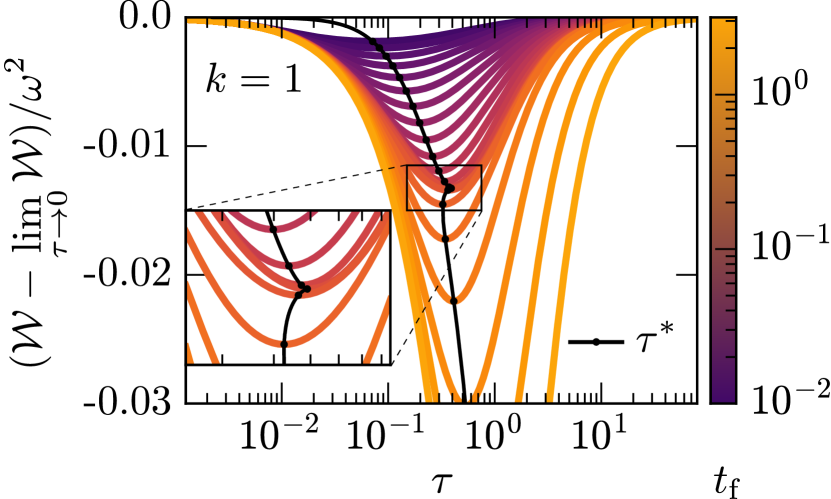
Figure 2: The work of the closed-loop protocol averaged over the measured values $v_{0}$ shows a pronounced minimum for a finite persistence time $\tau$; here shown for $k=1$ and $t_{\text{f}}\in[10^{-2},10^{0.5}]$. The $y$-axis shows the reduction in average work compared to the passive limit ($\tau\to 0$). Inset shows the kink in the minimum $\tau$ (black line) as a function of $t_{\text{f}}$.

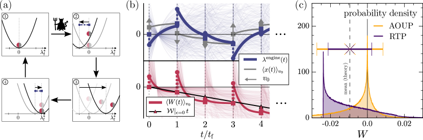
Figure 3: Active information engine: (a) cyclic protocol $\lambda^{\mathrm{engine}}$ determined upon an initial self-propulsion measurement $v_{0}$ in each cycle, (b) single realisation of cyclic engine protocol (thick blue), corresponding noise-averaged particle position (grey), and cumulative work (thick red). The arrows indicate the velocity measurements. Thin lines show trajectories for other sequences of self-propulsion measurements ($\omega=1.0,\tau=0.5,t_{\text{f}}=10,k=0.5$). (c) Work distribution per cycle for AOUP and RTP from simulations ($\omega=0.2,\tau=1,t_{\text{f}}=10,k=2$). While the mean ($\times$) is identical for AOUP and RTP and matches the theory (dashed line), AOUPs have a larger standard deviation (vertical bars); indicating that a motor run with RTPs is more precise. Moreover, for RTPs, the unique mode of the distribution is below the mean value, while it is close to zero for AOUPs.

Active information engine.—A notable application of optimal closed-loop protocols are optimized cyclic machines. Based on our results so far, one can readily construct a minimal, optimal information engine that harvests energy from the activity using self-propulsion measurements, as follows. Starting from Eqs. (5)-(9), we perform a secondary optimization of $\left\langle W\right\rangle_{v_{0}}$ with respect to $\lambda_{\text{f}}$, obtaining that the optimal target distance after measuring $v_{0}$ is $\lambda_{\text{f}}=\frac{1}{k+\tau^{-1}}+\frac{1}{2}\tau v_{0}(1-e^{-t_{\text{f}}/\tau})$, so that $d=0$. Thus, $\left\langle W\right\rangle_{v_{0}}\leq 0$ for all $v_{0}$. Setting $d=0$ in Eq. (5) gives the corresponding optimal protocol $\lambda^{\mathrm{engine}}$,

$$\lambda^{\mathrm{engine}}=\left\{\begin{array}[]{l l}0,&t=0\\ \frac{\tau v_{0}}{2}\left(\frac{3+k\tau}{1+k\tau}-\frac{1+k\tau}{k\tau}e^{-t/\tau}\right)&0<t<t_{\text{f}}\\ \frac{\tau v_{0}}{2}\left(\frac{3+k\tau}{1+k\tau}-e^{-t_{\text{f}}/\tau}\right)&t=t_{\text{f}}\end{array}\right.\ .$$ (11)

Iterating $\lambda^{\mathrm{engine}}$ yields a cyclic engine with period $t_{\text{f}}$, as visualized in Fig. 3. The motor builds up nontrivial correlations between the cycles. However, we can nevertheless access the average work extraction per cycle, by reasoning as follows. First, the orientational dynamics is not affected by the trap, so that all $v_{0}$ measurements are simply drawn from its steady state. Second, the final trap position now automatically coincides with the average particle position at the end of the protocol, so that the protocol extracts any average potential energy build-up during the process. Therewith, we can readily obtain from Eq. (9) the average work extraction per cycle $-\frac{k}{2(k+\tau^{-1})^{2}}\omega^{2}-\frac{1}{8}\tau\omega^{2}\left(1-e^{-2t_{\text{f}}/\tau}\right),$ both for AOUPs and RTPs , which has no optimum value of $\tau$, and reaches its maximum in the quasistatic regime. We find that, while the average work is identical for AOUPs and RTPs, the work distributions differ significantly, Fig. 3(c). Most significantly, the maximum value of the distribution is at a negative value below the average for RTPs, whereas it is around zero for AOUPs .

Finally, we address the effect of measurement uncertainty on the extractable work, and the thermodynamic cost of the information acquisition Sagawa and Ueda (2010); Kullback et al. (2013); Cao and Feito (2009); Parrondo et al. (2015), which has not been included in previous studies of active information engines Cocconi et al. (2023). Since the closed-loop protocol relies on a measurement, its associated uncertainty prevents the controller from applying the optimal protocol accurately and thus from extracting the maximum available work. Assuming that the $v$ measurement has a Gaussian-distributed error $\epsilon$, we show in Schüttler et al. that the net extracted work has an additional cost term $\Delta\mathcal{W}(\epsilon)\propto\epsilon^{2}$, leading to a total average work extraction per cycle of

$$\mathcal{W}^{\mathrm{engine}}=-\frac{k\omega^{2}}{2(k+\tau^{-1})^{2}}-\frac{\tau\omega^{2}}{8}\left(1-e^{-2t_{\text{f}}/\tau}\right)+\Delta\mathcal{W}(\epsilon)\,.$$ (12)

The cost term $\Delta\mathcal{W}(\epsilon)\geq 0$ reaches its highest value of $\tau\epsilon^{2}/2$ in the quasi-static limit and is identical for RTPs and AOUPs, despite the different $v$ distributions.

The information-efficiency of the engine is obtained by dividing the mean extracted work per cycle by the information acquisition cost,

$$\eta=\frac{-\mathcal{W}^{\mathrm{engine}}}{D_{v}\,\Delta\mathcal{I}}\,.$$ (13)

For an individual measurement, the information acquisition costs are given by the relative entropy, and when averaged over multiple cycles, by the mutual information $\Delta\mathcal{I}$ between the true value $v_{0}^{\mathrm{r}}$ and the measurement outcome $v_{0}^{\mathrm{m}}$ Sagawa and Ueda (2010, 2008); Cao and Feito (2009); Abreu and Seifert (2011). Here, the information-theoretical contribution is scaled by $D_{v}$, which plays the role of “temperature” of the random variable.

As we explicitly show in Schüttler et al. , the mutual information for AOUPs is

$$\Delta\mathcal{I}_{\mathrm{AOUP}}[v_{0}^{\mathrm{m}}:v_{0}^{\mathrm{r}}]=\frac{1}{2}\ln\left(1+\frac{{\omega}^{2}}{\epsilon^{2}}\right).$$ (14)

As expected, it vanishes for $\epsilon\to\infty$, where measurements become useless, and diverges for $\epsilon\to 0$. This divergence is not surprising, in view of the infinite information content in a continuous variable, $v_{0}\in\mathbb{R}$ Polyanskiy and Wu (2014); Gray (2011). For RTPs, we find that in the regime of small errors $\epsilon\ll\omega$,

$$\Delta\mathcal{I}_{\mathrm{RTP}}[v_{0}^{\mathrm{m}}:v_{0}^{\mathrm{r}}]=\ln(2)\,.$$ (15)

Thus, the measurement yields exactly one bit of information. Comparing (15) and (14) indicates that, at least for modest measurement uncertainty, which is the regime of interest, the cost of information acquisition is always smaller for RTPs than for AOUPs. In fact, RTPs have the smallest information cost (one bit) of any possible active particle model. Recalling that the extractable work is independent of the model of self-propulsion, we conclude that the information efficiency $\eta$ is always highest for RTPs.

Together with Eqs. (12) and (15), this gives a universal upper bound to the information-efficiency,

$$\eta\leq\eta_{\mathrm{max}}={1}/{[4\ln(2)]}\,.$$ (16)

The engine is most efficient when run with an RTP at low frequency $1/t_{\text{f}}$, with low error $\epsilon$, and $k\tau=1$ . Finally, we note that even for finite $t_{\text{f}}$, the efficiency $\eta$ admits a maximum at a finite persistence time $\tau$.

Conclusions.—We have generalized a canonical optimization problem to the case of active particles. The open-loop protocol is not affected by activity, but flucutations of the work are generally increased. In constrast, closed-loop protocols can extract energy from self-propulsion measurements by jumps away from the target position. Surprisingly, a finite persistence time is beneficial as compared to “infinitely persistent” (ballisitic) particles. We have further derived an optimal engine to harvest work from the self-propulsion measurements by simple shifts of the trap. Such engine is most efficient and most precise for RTPs, i.e., it benefits from non-Gaussianity. We found a universal upper efficiency bound for this design of engine of $1/[4\ln(2)]\approx 0.36$. Higher efficiencies can presumably be reached with more complicated machines, for instance by dynamically adjusting the trap stiffness.

To find optimal solutions for more complicated processes, one may apply recent machine-learning algorithms Whitelam (2023); Engel et al. (2023); Loos et al. (2024). With such, also collective active systems could be studied. Our results for AOUPs readily generalize to higher dimensions, and it would be interesting to explore RTPs and other active matter models in higher dimensions as well.

Our insights are complementary to recent progress on optimal control of active matter using a perturbative framework based on response theory Davis et al. (2024); Gupta et al. (2023). While this framework provides a general approach applicable to more complicated scenarios, it applies only to the regime of slow and weak driving. Instead, we have focused on the fast driving regime, allowing us to explicitly study the emergence of driving discontinuities, which play a crucial role in all our optimal protocols. As opposed to an active ratchet, the information-driven work extraction minimises dissipation from unprofitable non-equilibrium fluctuations during the initial correlation time.

We thank Robert Jack and Édgar Roldán for insightful discussions. R.G.-M. acknowledges support from a St John’s College Research Fellowship, Cambridge. J.S. acknowledges funding through the UK Engineering and Physical Sciences Research Council (Grant number 2602536). S.L. acknowledges funding through the postdoctoral fellowship of the Marie Skłodowska-Curie Actions (Grant Ref. EP/X031926/1) undertaken by the UKRI, through the Walter Benjamin Stipendium (Project No. 498288081) from the Deutsche Forschungsgemeinschaft (DFG), and from Corpus Christi College Cambridge.

References

- Schneider and Stark (2019) Elias Schneider and Holger Stark, “Optimal steering of a smart active particle,” Europhysics Letters 127, 64003 (2019).
- Falk et al. (2021) Martin J Falk, Vahid Alizadehyazdi, Heinrich Jaeger, and Arvind Murugan, “Learning to control active matter,” Physical Review Research 3, 033291 (2021).
- Liebchen and Löwen (2019) Benno Liebchen and Hartmut Löwen, “Optimal navigation strategies for active particles,” Europhysics Letters 127, 34003 (2019).
- Baldovin et al. (2023) Marco Baldovin, David Guéry-Odelin, and Emmanuel Trizac, “Control of active Brownian particles: An exact solution,” Phys. Rev. Lett. 131, 118302 (2023).
- Shankar et al. (2022) Suraj Shankar, Vidya Raju, and L Mahadevan, “Optimal transport and control of active drops,” Proceedings of the National Academy of Sciences 119, e2121985119 (2022).
- Davis et al. (2024) Luke K Davis, Karel Proesmans, and Étienne Fodor, “Active matter under control: Insights from response theory,” Physical Review X 14, 011012 (2024).
- Gupta et al. (2023) Deepak Gupta, Sabine HL Klapp, and David A Sivak, “Efficient control protocols for an active ornstein-uhlenbeck particle,” arXiv preprint arXiv:2304.12926 (2023).
- Aurell et al. (2011) Erik Aurell, Carlos Mejía-Monasterio, and Paolo Muratore-Ginanneschi, “Optimal protocols and optimal transport in stochastic thermodynamics,” Physical Review Letters 106, 250601 (2011).
- Ekeh et al. (2020) Timothy Ekeh, Michael E Cates, and Étienne Fodor, “Thermodynamic cycles with active matter,” Physical Review E 102, 010101 (2020).
- Majumdar et al. (2022) Rita Majumdar, Arnab Saha, and Rahul Marathe, “Exactly solvable model of a passive Brownian heat engine and its comparison with active engines,” Journal of Statistical Mechanics: Theory and Experiment 2022, 073206 (2022).
- Blaber and Sivak (2023) Steven Blaber and David A Sivak, “Optimal control in stochastic thermodynamics,” Journal of Physics Communications 7, 033001 (2023).
- Lee et al. (2023) Hyun Keun Lee, Youngchae Kwon, and Chulan Kwon, “Nonequilibrium thermodynamics for a harmonic potential moving in time,” Journal of the Korean Physical Society 83, 331–336 (2023).
- Malgaretti and Stark (2022) Paolo Malgaretti and Holger Stark, “Szilard engines and information-based work extraction for active systems,” Physical Review Letters 129, 228005 (2022).
- Cocconi et al. (2023) Luca Cocconi, Jacob Knight, and Connor Roberts, “Optimal power extraction from active particles with hidden states,” Physical Review Letters 131, 188301 (2023).
- Schmiedl and Seifert (2007) Tim Schmiedl and Udo Seifert, “Optimal finite-time processes in stochastic thermodynamics,” Physical Review Letters 98, 108301 (2007).
- Engel et al. (2023) Megan C Engel, Jamie A Smith, and Michael P Brenner, “Optimal control of nonequilibrium systems through automatic differentiation,” Physical Review X 13, 041032 (2023).
- Whitelam (2023) Stephen Whitelam, “Demon in the machine: learning to extract work and absorb entropy from fluctuating nanosystems,” Physical Review X 13, 021005 (2023).
- Loos et al. (2024) Sarah A. M. Loos, Samuel Monter, Felix Ginot, and Clemens Bechinger, “Universal symmetry of optimal control at the microscale,” Physical Review X 14, 021032 (2024).
- Parrondo et al. (2015) Juan MR Parrondo, Jordan M Horowitz, and Takahiro Sagawa, “Thermodynamics of information,” Nature physics 11, 131–139 (2015).
- Abreu and Seifert (2011) David Abreu and Udo Seifert, “Extracting work from a single heat bath through feedback,” Europhysics Letters 94, 10001 (2011).
- Saha et al. (2021) Tushar K Saha, Joseph NE Lucero, Jannik Ehrich, David A Sivak, and John Bechhoefer, “Maximizing power and velocity of an information engine,” Proceedings of the National Academy of Sciences 118, e2023356118 (2021).
- Cocconi and Chen (2024) Luca Cocconi and Letian Chen, “Efficiency of an autonomous, dynamic information engine operating on a single active particle,” Physical Review E 110, 014602 (2024).
- Krishnamurthy et al. (2016) Sudeesh Krishnamurthy, Subho Ghosh, Dipankar Chatterji, Rajesh Ganapathy, and AK Sood, “A micrometre-sized heat engine operating between bacterial reservoirs,” Nature Physics 12, 1134–1138 (2016).
- Holubec et al. (2020) Viktor Holubec, Stefano Steffenoni, Gianmaria Falasco, and Klaus Kroy, “Active Brownian heat engines,” Physical Review Research 2, 043262 (2020).
- Fodor and Cates (2021) Étienne Fodor and Michael E Cates, “Active engines: Thermodynamics moves forward,” Europhysics Letters 134, 10003 (2021).
- Speck (2022) Thomas Speck, “Efficiency of isothermal active matter engines: Strong driving beats weak driving,” Physical Review E 105, L012601 (2022).
- Zakine et al. (2017) Ruben Zakine, Alexandre Solon, Todd Gingrich, and Frédéric Van Wijland, “Stochastic stirling engine operating in contact with active baths,” Entropy 19, 193 (2017).
- Sagawa and Ueda (2010) Takahiro Sagawa and Masahito Ueda, “Generalized Jarzynski equality under nonequilibrium feedback control,” Physical Review Letters 104, 090602 (2010).
- Kullback et al. (2013) Solomon Kullback, John C Keegel, and Joseph H Kullback, Topics in statistical information theory, Vol. 42 (Springer Science & Business Media, 2013).
- Cao and Feito (2009) Francisco J Cao and M Feito, “Thermodynamics of feedback controlled systems,” Physical Review E 79, 041118 (2009).
- Schnitzer et al. (1990) M Schnitzer, S Block, H Berg, and Purcell E, “Strategies for chemotaxis,” Biology of the chemotactic response 46, 15 (1990).
- Schnitzer (1993) Mark J Schnitzer, “Theory of continuum random walks and application to chemotaxis,” Physical Review E 48, 2553 (1993).
- Cates (2012) Michael E Cates, “Diffusive transport without detailed balance in motile bacteria: does microbiology need statistical physics?” Reports on Progress in Physics 75, 042601 (2012).
- Garcia-Millan and Pruessner (2021) Rosalba Garcia-Millan and Gunnar Pruessner, “Run-and-tumble motion in a harmonic potential: field theory and entropy production,” Journal of Statistical Mechanics: Theory and Experiment 2021, 063203 (2021).
- Lee and Park (2022) Jae Sung Lee and Hyunggyu Park, “Effects of the non-markovianity and non-gaussianity of active environmental noises on engine performance,” Physical Review E 105, 024130 (2022).
- Jarzynski (1997) Christopher Jarzynski, “Nonequilibrium equality for free energy differences,” Physical Review Letters 78, 2690 (1997).
- Crooks (1998) Gavin E Crooks, “Nonequilibrium measurements of free energy differences for microscopically reversible Markovian systems,” Journal of Statistical Physics 90, 1481–1487 (1998).
- Gaspard and Kapral (2017) Pierre Gaspard and Raymond Kapral, “Communication: Mechanochemical fluctuation theorem and thermodynamics of self-phoretic motors,” The Journal of chemical physics 147 (2017).
- Pietzonka and Seifert (2017) Patrick Pietzonka and Udo Seifert, “Entropy production of active particles and for particles in active baths,” Journal of Physics A: Mathematical and Theoretical 51, 01LT01 (2017).
- Speck (2018) Thomas Speck, “Active Brownian particles driven by constant affinity,” Europhysics Letters 123, 20007 (2018).
- (41) Janik Schüttler, Rosalba Garcia-Millan, Michael E Cates, and Sarah A M Loos, In preparation .
- Note (1) We can assume that the particle has equilibrated by the end of the cycle if its duration is greater than the timescales and , so that the particle position has effectively reached its steady state, and we can thus apply Eq. (9).
- Note (2) At long timescales, the center of the trap performs a diffusive motion. This diffusive delocalization can be prevented at the cost of lowering the work extraction by modifying the protocol, for instance, by resetting the engine to the origin at the end of each cycle. This process is described by Eqs. (5)-(9) with . If is sufficiently long, the engine still produces net work.
- Sagawa and Ueda (2008) Takahiro Sagawa and Masahito Ueda, “Second law of thermodynamics with discrete quantum feedback control,” Physical Review Letters 100, 080403 (2008).
- Polyanskiy and Wu (2014) Yury Polyanskiy and Yihong Wu, “Lecture notes on information theory,” Lecture Notes for ECE563 (UIUC) (2014).
- Gray (2011) Robert M Gray, Entropy and information theory (Springer Science & Business Media, 2011).
- Note (3) Taking into account the underlying thermodynamic cost of the self-propulsion as a background dissipation term results in a maximum efficiency at some finite frequency . Specifically, assuming a constant rate of ATP depletion of the self-propulsion mechanism, the efficiency peaks at a finite .