Coevolutionary game dynamics with localized environmental resource feedback

Abstract

Dynamic environments shape diverse dynamics in evolutionary game systems. We introduce spatial heterogeneity of resources into the Prisoner’s Dilemma Game model to explore the co-evolution of individuals’ strategies and environmental resources. The adequacy of resources significantly affects the survival competitiveness of surrounding individuals. Feedback between individuals’ strategies and the resources they can use leads to the dynamic of the “oscillatory tragedy of the commons”. Our findings indicate that when the influence of individuals’ strategies on the update rate of resources is significantly high, individuals can form sustained spatial clustered patterns. These sustained patterns can directly trigger a transition in the system from the persistent periodic oscillating state to an equilibrium state. These findings align with observed phenomena in real ecosystems, where organisms organize their spatial structures to maintain system stability. We discuss critical phenomena in detail, demonstrating that the aforementioned phase transition is robust across various system parameters including: the strength of cooperators in restoring the environment, the initial distributions of cooperators, and noise.

I Introduction

Coevolutionary game dynamics with environmental feedback are topics of great concern in complex system science. In an ecosystem with limited public goods, individuals will inevitably defect in pursuit of their own benefits, ultimately depleting available resources. Hardin called this dilemma “the tragedy of the commons” (TOC), and he mentioned that there is no technical solution for this dilemma[1]. Recently, Weitz et al. studied a class of dynamics which was named “oscillatory tragedy of the common” (o-TOC) with the consideration of payoffs with environmental feedback[2]. Defectors destroy environment and cooperators restore it. Thus, system cycles between deplete and replete environmental states and cooperation and defection behavior states. Because individuals tend to choose cooperation in deplete state and defection in replete state respectively in order to get higher payoff. For instance, overgrazing degrades grasslands, which can be restored if pastoralists control grazing[2]. Tilman et al. proposed a comprehensive framework for eco-evolutionary games, providing examples and analyzing the dynamic mechanisms underlying the oscillation phenomena[3]. They theoretically deduced the conditions for the avoidance of the oscillatory tragedy[2, 3].

However, the aforementioned studies assumed a uniform environment, which may not accurately reflect the real-world systems. Spatial heterogeneity of environment was already taken into consideration in studies of ecosystems such as mussel bed, arid ecosystems and bacterial colonies[4, 5, 6]. Compared to non-spatial models, spatial interactions can significantly affect system stability and promote the formation of spatial patterns[7]. Game transitions can effectively promote cooperation rate, which represent the effect of localized environmental feedback in evolutionary games, and it is related to the idea of partner-fidelity feedback in evolutionary biology like grass-endophyte mutualism[8, 9, 10, 11, 12, 13]. Other researchers have also utilized game transitions to investigate the affection of game information, reinforcement learning individuals and state-dependent strategies[14, 15, 16]. Lin et al. considered spatiotemporal dynamics with environmental diffusion in individual based model and analyzed dynamic mechanism of o-TOC[17]. Hauert et al. investigated asymmetric evolutionary games in heterogeneous environment that consists of patches of different qualities and found a series of dynamic phenomena[18]. In summary, heterogeneous environmental feedback has significant influence on evolutionary games that cannot be ignored.

Thus, in this work, we introduce spatial heterogeneous resources into the Prisoner’s Dilemma Game model with environmental feedback. Environmental resources are assigned to nodes in square lattices which can be used by individuals on adjacent nodes. System oscillates between deplete and replete states of resources because individuals tend to cooperate in nodes with sufficient resources and defect in nodes with deficient resources, respectively. When the update rate of resource is sufficiently high, sustained clustered patterns emerge in the distributions of strategies and resources, leading to a phase transition from the oscillating state to an equilibrium state.

II Model and simulations

We study the evolutionary dynamics of $2\times 2$ games in square lattice with $N=L\times L$ nodes and periodic boundary conditions. Every individual $i$ takes up a node alone and has a strategy $s_{i}\in\{C,D\}$, $i=1,2,...,N$. $C$ stands for cooperation and $D$ stands for defection. Initially, individuals’ strategies is randomly assigned as cooperation with equal probability $x_{C0}$ or defection with probability $1-x_{C0}$. Each individual $i$ is assigned a certain amount of resources, represented by the parameter $e_{i}\in[0,1]$. $e_{i}=0$ means node $i$ has the poorest resources, and $e_{i}=1$ means node $i$ has the most abundant resources. Individuals can use their own and their neighbors’ resources. Thus, the total resources individual $i$ can use are

$$n_{i}=0.5\times e_{i}+0.125\times(e_{a}+e_{b}+e_{c}+e_{d}),$$ (1)

$a,b,c,d$ are the neighbors of individual $i$, and $e_{a},e_{b},e_{c},e_{d}$ are their resources respectively. When individual $i$ plays games with their neighbors, its payoff is determined by $n_{i}$ and the following payoff matrices:

$$\Pi_{i}=(1-n_{i})\times A_{0}+n_{i}\times A_{1},$$ (2)

where $A_{0}$ and $A_{1}$ are the matrices which correspond to situations of resource scarcity and resource abundance respectively. $A_{1}$ represents the payoff matrix of the Prisoner’s Dilemma Game which is used when resources are abundant, $A_{0}$ corresponds to the payoff matrix that benefits cooperators when individuals deplete their resources, respectively. The advantage of cooperators in $A_{0}$ arises because cooperators can regenerate resources in hostile environments.

$$A_{0}=\begin{bmatrix}R_{0}&S_{0}\\ T_{0}&P_{0}\\ \end{bmatrix},\quad A_{1}=\begin{bmatrix}R_{1}&S_{1}\\ T_{1}&P_{1}\\ \end{bmatrix},$$ (3)

where $R_{0}$($R_{1}$) denotes the reward of cooperation, $S_{0}$($S_{1}$) denotes the sucker’s payoff, $T_{0}$($T_{1}$) denotes the temptation to cheat, $P_{0}$($P_{1}$) denotes the punishment for mutual defection.

At each step $\tau$, we randomly choose an individual $i$ to play games with its neighbors and update its strategy $s_{i}$ to $s_{i^{\prime}}$ by myopic rules[19, 20, 21] with probability

$$P(s_{i^{\prime}}\to s_{i})=\frac{1}{1+e^{(\frac{\pi_{i}-\pi_{i^{\prime}}}{k})}},$$ (4)

where $\pi_{i}$ is the average payoff of individual $i$’s games with four neighbors, $s_{i^{\prime}}$ is the opposed strategy of $s_{i}$, $\pi_{i^{\prime}}$ is the average payoff of individual $i$ with strategy $s_{i^{\prime}}$, $k$ controls the noise. After updating individual $i$’s strategy $s_{i}(\tau)$ to $s_{i}(\tau+1)$, we update node $i$’s and its neighbors’ resources

$$e_{j}(\tau+1)=\begin{cases}e_{j}(\tau)+\alpha\mu\theta\qquad s_{i}(\tau+1)=C,\\ e_{j}(\tau)-\alpha\mu\qquad\enspace s_{i}(\tau+1)=D,\\ \end{cases}$$ (5)

$j=i,a,b,c,d$. $\mu\in[0,1]$ is the parameter that controls the update rate of resources relative to the update rate of strategies. $\theta\in(0,1/\mu]$ denotes the strength of cooperators in restoring the environment. $\alpha=0.5$ when $j=i$ and $\alpha=0.125$ when $j=a,b,c,d$. We restrict $e_{i}\in[0,1]$ while updating resources. If $e_{i}$ should be updated to a value bigger than 1 according to Eq. (5), we set it to 1. Similarly, if $e_{i}$ should be updated to a value less than 0, we set it to 0. We take $N$ steps with chances to update strategies and resources as a Monte Carlo(MC) step, every individual has equal chance to update its strategy once in each MC step.

The fraction of cooperators is defined as

$$x_{C}=\frac{1}{N}\sum_{i=1}^{N}\delta(s_{i}-C),$$ (6)

where $\delta(s_{i}-C)=1$ when $s_{i}=C$, $\delta(s_{i}-C)=0$ when $s_{i}=D$. The average resources of the system is

$$e=\frac{1}{N}\sum_{i=1}^{N}e_{i}.$$ (7)

We use these two parameters to discuss the co-evolution of the cooperation level and the average resources of the system. In our simulations, without loss of generality, we set noise $k=0.01$ and system size $N=L\times L=400\times 400$. The payoff matrices are

$$A_{0}=\begin{bmatrix}\enspace 5&\enspace 2\enspace\\ \enspace 4&\enspace 2\enspace\\ \end{bmatrix},\quad A_{1}=\begin{bmatrix}\enspace 5&\enspace 0\enspace\\ \enspace 6&\enspace 2\enspace\\ \end{bmatrix}.$$ (8)

In our results of Monte Carlo simulations, the initial probability for individuals to cooperate is $x_{C0}=0.2$, the initial resource of nodes are all set to $e_{0}=0.3$.

III Results and discussion

III.1 Oscillating dynamics

Figure 1: Four states of the oscillating phase plane dynamics of $x_{C}-e$ system, represented by the distributions of the system for $\theta=1.5$ and $\mu=0.007$ at (a), (b) $t=19846$; (c), (d) $t=19864$; (e), (f) $t=19883$; and (g), (h) $t=19900$. (a), (c), (e), (g) Distributions of cooperators (black pixels) and defectors (gray pixels). (b), (d), (f), (h) Distributions of environmental resources of nodes in the system. (i) Time evolution of the fraction of cooperators and the average resources of the system from $t=19500$ to $t=20000$. The aforementioned four states are marked by four vertical red dashed lines in order from left to right. (j) Phase plane dynamics of $x_{C}-e$ system from $t=19500$ to $t=20000$. The regions of the above four states are marked with red circles.

Figure 2: Simulation results with different evolutionary dynamics for $\theta=2.0$ and different update rate of resources (a)-(d) $\mu=0.005$, (e)-(h) $\mu=0.016$, and (i)-(l) $\mu=0.04$, respectively. (a), (e), (i) Time evolutions of the fraction of cooperators and the average resources of the system. (b), (f), (j) Phase plane dynamics of $x_{C}-e$ system. (c), (g), (k) Distributions of cooperators (black pixels) and defectors (white pixels). (d), (h), (l) Distributions of environmental resources of nodes in the system.

Figure 3: Individual’s probability of cooperation as a function of usable resources $n_{i}$ for different numbers of cooperative neighbors $g=0,1,2,3,4$.

From Fig. 1 we can see that the system exhibits persistent oscillating dynamics of the fraction of cooperators $x_{C}$ and the average resources of the system $e$. Upon reaching a periodic oscillating state, the system cycles through four distinct states within each period: (1) deficient resources and low fraction of cooperators ($x_{C,\mathrm{min}}$, $e_{\mathrm{min}}$), (2) deficient resources and high fraction of cooperators ($x_{C,\mathrm{max}}$, $e_{\mathrm{min}}$), (3) sufficient resources and high fraction of cooperators ($x_{C,\mathrm{max}}$, $e_{\mathrm{max}}$), and (4) sufficient resources and low fraction of cooperators ($x_{C,\mathrm{min}}$, $e_{\mathrm{max}}$). Assuming the system initially starts in state 1, characterized by deficient environmental resources and dominance of defectors. Individuals gradually choose cooperation to obtain higher payoffs in the barren environment, and the environmental resources remain at a low level during this process, the system evolves to state 2. At this point, the dominant cooperators gradually restore sufficient environmental resources, leading the system to evolve to state 3, where cooperators maintain their dominant position. Moreover, individuals tend to choose defection for higher payoffs, and defectors quickly occupy almost the entire system before the environmental resources are significantly depleted, reaching state 4. After this, the environmental resources are gradually consumed by the defectors, returning the system to state 1. The distributions of the four states in Fig. 1 are taken from consecutive periods of time after the simulation has stabilized. They are marked by four vertical red dashed lines in the time series of Fig. 1(j) in order from left to right. Figs. 2(a) and 2(b) illustrate the time series and phase space of the fraction of cooperators and the average resources of the system, respectively. In Fig. 2(b), the phase trajectory exhibits a periodic rotation within a region similar to an irregular rounded quadrilateral, the four vertices regions of the quadrilateral correspond to the four states described above (they are also shown more clearly in Fig. 1(j)). This behavior is analogous to the o-TOC dynamics described in Ref. [2]. Individuals tend to choose cooperation when resources are deficient and defection when resources are sufficient to maximize their immediate payoff. Additionally, the interplay between cooperators’ production and defectors’ consumption of resources drives the system through these cyclical states.

According to the myopic rule (see Eq. (4)), the probability of cooperation is not influenced by individuals’ previous strategies. Based on Eqs. (1) - (4), given the neighbors’ strategies and the total amount of resources available to the individuals, the individuals’ probability of cooperation can be calculated, as shown in Fig 3. The probability of choosing cooperation decreases as an individual’s available resources increase. Furthermore, an individual’s propensity to cooperate diminishes rapidly to nearly zero when the average resources of the system approaches a critical value determined by the number of cooperative neighbors $g$ (see Fig. 3). This mechanism further explains the observed oscillations: cooperators tend to defect when resources are sufficient or when there are fewer cooperative neighbors, while defectors are inclined to cooperate when resources are deficient or when more neighbors are cooperative. Thus, the system orderly cycles through the aforementioned four states: ($x_{C,\mathrm{min}}$, $e_{\mathrm{min}}$), ($x_{C,\mathrm{max}}$, $e_{\mathrm{min}}$), ($x_{C,\mathrm{max}}$, $e_{\mathrm{max}}$), and ($x_{C,\mathrm{min}}$, $e_{\mathrm{max}}$). Distributions at $t=20000$ is shown in Figs. 2(c) and 2(d), clusters of cooperators and defectors appear, expand, and disappear rapidly and do not last.

III.2 Patterns and oscillations

Figure 4: Spiral patterns emerge in the simulation result for $\theta=2.0$ and $\mu=0.016$ at $t=13250$, which is in the transition stage between oscillatory transient state and equilibrium state. (a) Distribution of cooperators (black pixels) and defectors (white pixels). (b) Distribution of environmental resources of nodes in the systems. The parameter conditions used in this figure produce results consistent with Fig. 2 (e)-(h), with the eventual emergence of the clustered patterns driving the system to evolve to the equilibrium state.

When we keep the value of $\theta$ constant, an significant increase in the update rate of resources $\mu$ results in the disappearance of the previously observed persistent oscillations (see Figs. 2(a), 2(b), 2(e) and 2(f)). As shown in Figs. 2(e) and 2(f), after several periods, the system transitions from an oscillating transient state to an equilibrium state. In the time series, the amplitudes of the fluctuations rapidly decrease within a short period, eventually resulting in only minor fluctuations (see Fig. 2(e)). Following several periodic rotations, the phase trajectory gradually converges towards the center (see Fig. 2(f)). Figs. 2(g) and 2(h) display clustered patterns clearly in the spatial distributions of strategies and resources. We demonstrate that these clustered patterns account for the emergence of the equilibrium state. The oscillating state is transient; once spatial patterns begin to form, the amplitude of the time series gradually decreases. The duration of the oscillating transient state is unstable, and under the same parameters, different systems generate spatial clustered patterns and enter the equilibrium state at different rates. Additionally, spiral patterns appear at the beginning of the transformation process (see Figs. 4(a) and Figs. 4(b)). These spirals eventually couple and form clustered patterns, leading the system into an equilibrium state characterized by only slight fluctuations in the time series, caused by the movements and deformations of these clusters. In our simulations, oscillations did not significantly influence the average fraction of cooperators, given the same other parameters.

Figure 5: Simulation results with different evolutionary dynamics for $\mu=0.015$ and different strength of cooperators in restoring the environment (a)-(d) $\theta=1.0$, (e)-(h) $\theta=2.0$, and (i)-(l) $\theta=4.0$, respectively. (a), (e), (i) Time evolutions of the fraction of cooperators and the average resources of the system. (b), (f), (j) Phase plane dynamics of $x_{C}-e$ system. (c), (g), (k) Distributions of cooperators (black pixels) and defectors (white pixels). (d), (h), (l) Distributions of environmental resources of nodes in the system.

To further investigate the relations among parameters, patterns, and oscillations, we conducted several groups of simulations for varying values of $\mu$ and $\theta$, some of which are shown in Figs. 2 and 5. When $\mu$ is sufficiently small, persistent oscillations occur without sustained spatial patterns (Figs.2(a) - 2(d)). Conversely, as $\mu$ increases, clustered patterns emerge and the system eventually reaches an equilibrium state (see Figs.2(e) - 2(h)). Further increases in $\mu$ result in smaller cluster sizes (see Figs.2(i) - 2(l)). By altering $\theta$, we observe different spatial distributions, including variations in the sizes of clustered patterns (see Figs.5(e) - 5(l)), and even the absence of sustained spatial patterns (see Figs.5(a) - 5(d)). In summary, increasing the update rate of resources $\mu$ triggers a phase transition from random unsustained patterns to sustained clustered spatial patterns, leading the system from the oscillating state to an equilibrium state. And the critical value $\mu_{C}$ is influenced by other parameters (see Fig. 6).

As we mentioned before, the clustered patterns are not entirely static, slight fluctuations in the time series and phase trajectories occur due to the movements and deformations of the clusters. Clusters of cooperators tend to migrate to nodes with deficient resources, while clusters of defectors move to nodes with sufficient resources. Cooperators produce resources in deficient nodes, whereas defectors consume resources in sufficient nodes. This local feedback dynamic leads to a dynamic equilibrium throughout the system. As clusters of cooperators and defectors move, the overall density of cooperators remains constant, thereby maintaining a fixed level of average resources of the system. Consequently, when $\mu$ exceeds the critical value, clustered patterns form, and the system reaches the equilibrium state. Our findings also indicate that systems with smaller clusters reach equilibrium faster (see Figs. 2(e) - 2(l) and 5(e) - 5(l)). It is important to note that spiral patterns in the transition stage from the oscillating state to the equilibrium state are not clear in systems with smaller clusters. These spiral patterns are small in size and evolve quickly, making them difficult to recognize. Based on the aforementioned dynamic equilibrium mechanism, local feedback dynamics within smaller clusters occur in a more confined area, accelerating evolutionary dynamics and leading to a quicker attainment of equilibrium. It is important to note that the phase transition described above can only occur in systems with sufficiently large spatial scales (i.e., a sufficient number of nodes). The above conclusions remains robust despite parameter variations including the strength of cooperators in restoring the environment and the initial distributions of cooperators. And we also prove that the above conclusions remains robust when the noise does not significantly affect the system (i.e., around the value $k=0.01$ used in this work).

Compared to the works of Weitz et al. and Tilman et al.[2, 3], our model exhibits similar oscillating dynamics of the fraction of cooperators and the average resources in the system. The system cycles orderly through the four aforementioned states (see Fig. 1 and Sec. III.1). However, they used replicator dynamics to investigate the coevolutionary game dynamics with environmental feedback and ignored the influence of spatial heterogeneity. The transitions from oscillating states to stable states in their works were directly induced by changes in dynamic stability caused by payoff matrices and other parameters. In contrast, the phase transition from the oscillating state to the equilibrium state in our work is driven by self-organized spatial clustered patterns of cooperators, defectors, and resources in the system. Under specific parameter conditions (see Fig. 6), spatial clustered patterns emerge, and the system evolves to the equilibrium state.

Hassell et al. found that lattice structures, spiral waves, and spatial chaos patterns effectively maintain population persistence in the host-parasitoid system under conditions of spatial heterogeneity and local movement patterns[22]. Although our work does not exhibit identical phenomena, both our findings and theirs illustrate similar self-organized criticality in complex systems with spatial heterogeneity. When their impact on environmental resources is potent enough, individuals can form spatial structures, such as clustered patterns, to counteract the oscillatory tragedy of the commons. Previous studies of real-world ecosystems have indeed demonstrated similar relations between spatial patterns and system stability[4, 23, 24, 25, 26]. However, the stability of ecosystems is affected by many complex factors at the same time. Our model, which did not consider the diffusion of resources or external influences but only the interaction of individuals with resources within a certain range around themselves, focuses on the co-evolution of two strategies and heterogeneous environmental resources, making it a simpler model for studying self-organized criticality. Importantly, we directly prove that sustained spatial patterns contribute to the formation of dynamic equilibrium, which enhances the stability of individual-based complex systems. Moreover, the system parameters affect the size and specific distributions of the persistent clusters, with systems featuring small-sized clusters tending to reach the equilibrium state faster in our results(see Figs. 2 and 5). This further illustrates the significant impact of clustered patterns on stability.

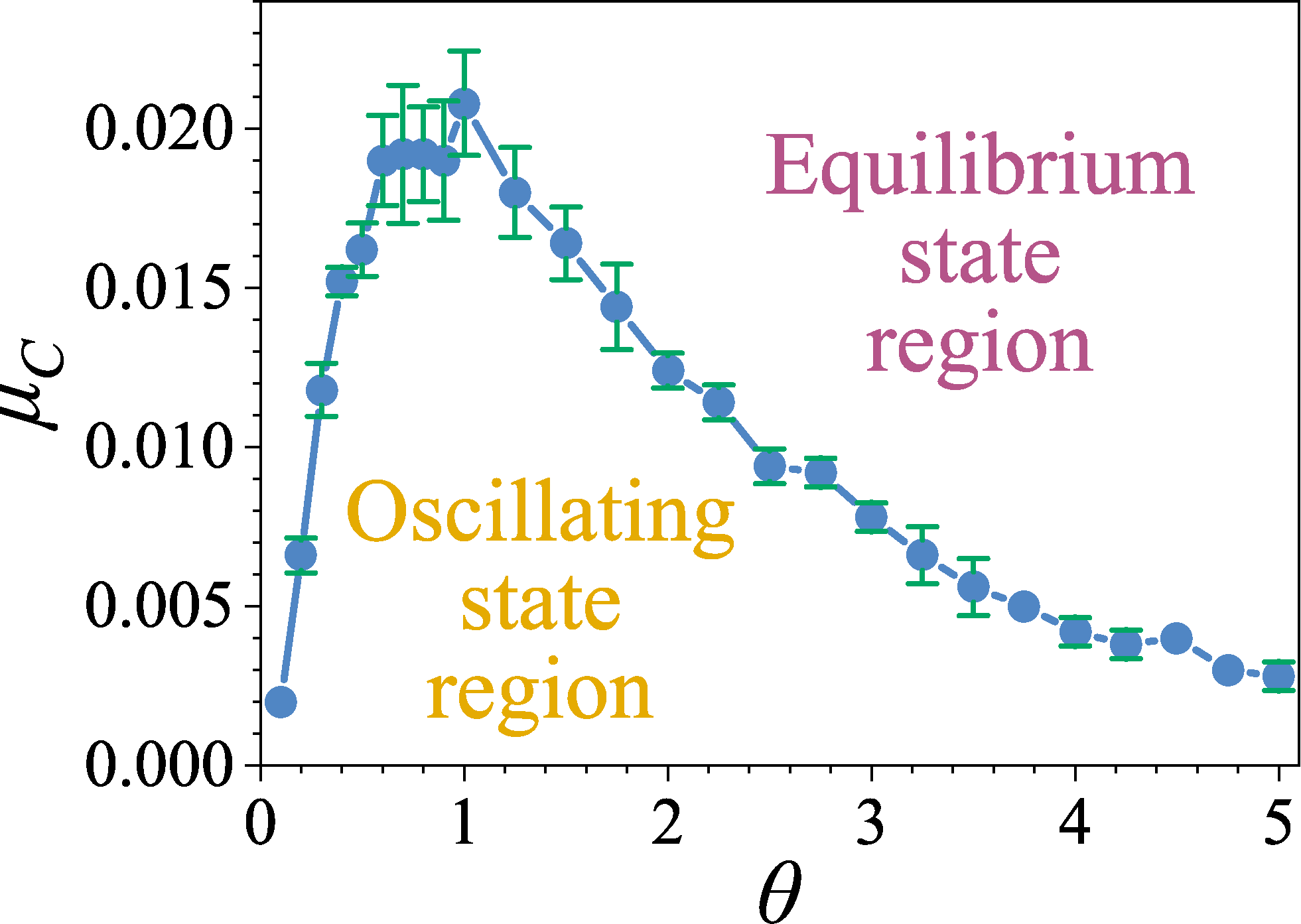
Figure 6: Critical values $\mu_{C}$ of the phase transition from the oscillating state to the equilibrium state as a function of parameter $\theta$. Each critical value $\mu_{C}$ is averaged over 50 repetitions.

As shown in Fig. 6, the critical value $\mu_{C}$ is correlated with $\theta$. Each critical value $\mu_{C}$ is averaged over 50 repetitions. The standard deviations of the critical values are within acceptable limits. In the phase space of $\theta$ and $\mu$, the region above the blue critical value curve is the equilibrium state region and the region below the curve is the oscillating state region. This figure further verifies the previous conclusion that, by keeping the value of $\theta$ constant while increasing the value of $\mu$, the system transitions from the oscillating state to the equilibrium state. Within the range of $(0,5.0]$ (noting that $\theta=0$ is meaningless), the critical value $\mu_{C}$ initially increases and then decreases as $\theta$ increases. The maximum $\mu_{C}$ occurs at $\theta=1.0$, where cooperators produce resources at the same rate that defectors consume them. As $|\theta-1.0|$ increases, the disparity between the rates of resource production by cooperators and consumption by defectors also increases, leading to a decrease in the critical value $\mu_{C}$. Thus, systems more easily enter the equilibrium state when individuals of one strategy have a speed advantage in influencing resources over others.

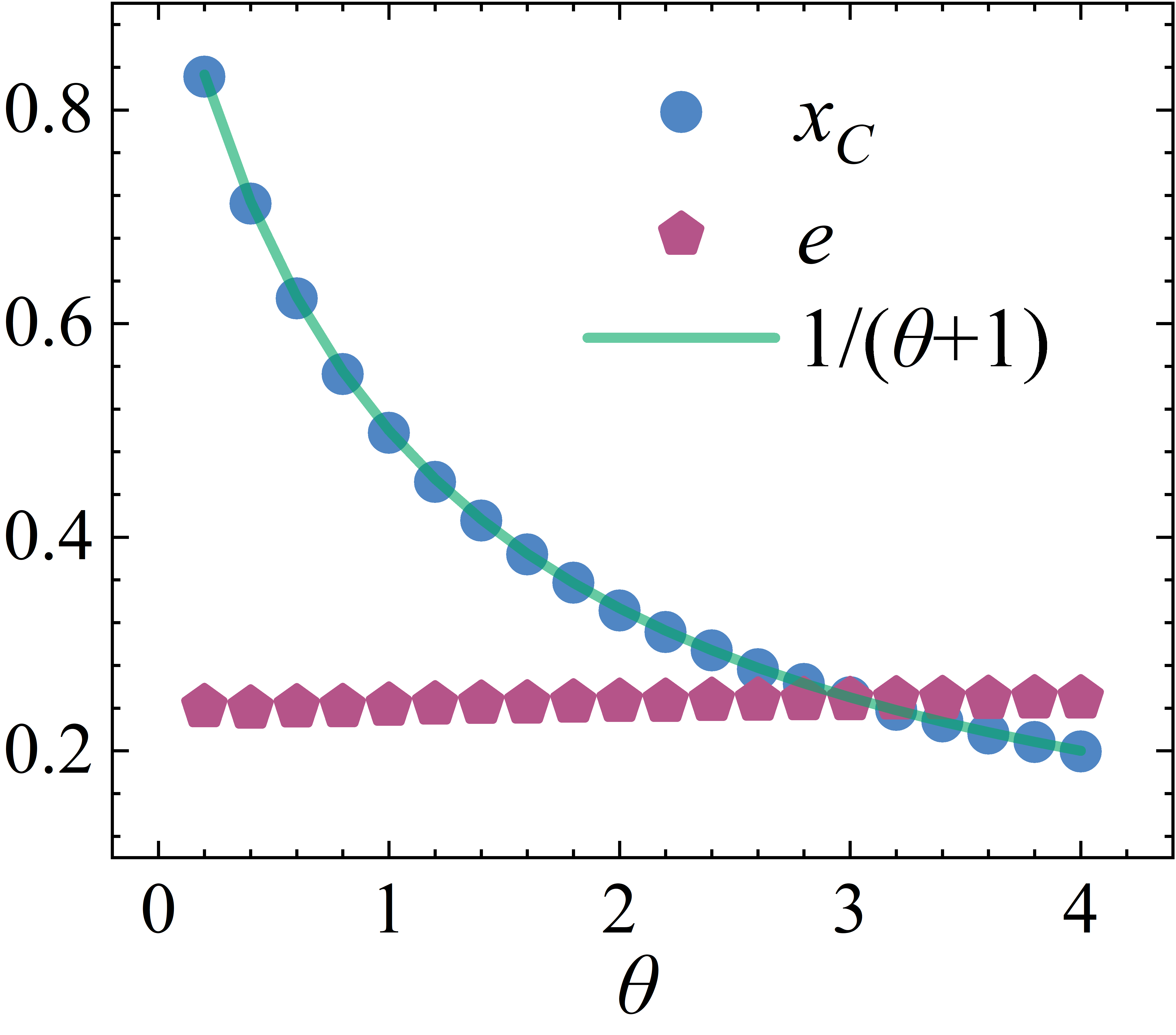
Figure 7: The fraction of cooperators and the average resources of the system as functions of $\theta$ for $\mu=0.002$. Each point of $x_{C}$ or $e$ is averaged over ten repeated simulations. The green line represents the theoretical approximate value of the fraction of cooperators calculated by Eq. (10).

For further analysis, we observed the average values of the fraction of cooperators and the average resources of the system across different $\theta$ values (see Fig. 7). The fraction of cooperators $x_{C}$ decreases rapidly as $\theta$ increases, while the average resources of the system $e$ remains relatively unchanged. This result suggests that individuals in the system tend to maintain environmental resources at an approximately fixed level, regardless of the proportion of cooperators and defectors, due to the parameter $\theta$. In our model, defectors consistently consume resources at a constant rate, whereas cooperators produce resources at a rate proportional to $\theta$. Consequently, the average variation of resources per MC step can be expressed as:

$$\Delta e=\mu(\theta x_{C}-(1-x_{C})).$$ (9)

Setting $\Delta e=0$ yields the fixed point for the fraction of cooperators:

$$x_{C}^{*}=\frac{1}{1+\theta}.$$ (10)

This theoretical prediction aligns well with the simulation results. Specifically, all the points representing the fraction of cooperators in the simulations fall on the curve given by $x_{C}^{*}=1/(1+\theta)$ (see Fig. 7).

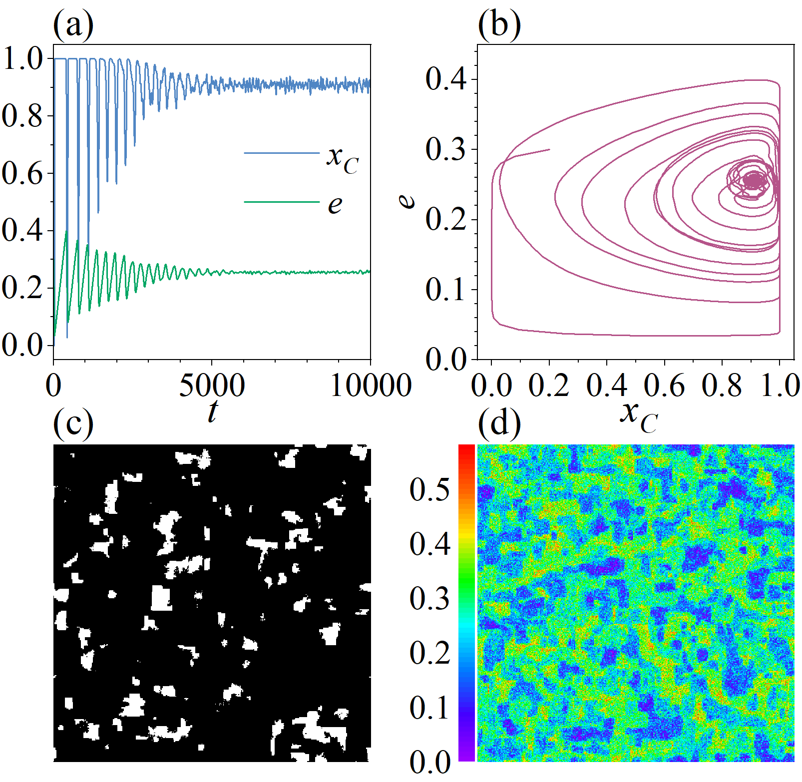
Figure 8: Equilibrium state and irregular block clusters emerge for $\theta=0.1$, $\mu=0.01$. (a) Time evolutions of fraction of cooperators and average resources of the system. (b) Phase plane dynamics of $x_{C}$-$e$ system. (c) Distribution of cooperators (black pixels) and defectors (white pixels). (d) Distribution of environmental resources of nodes in the system.

Based on the results in Fig. 7 and Eq. 10, the parameter $\theta$ influences the average fraction of cooperators, with $\theta=1.0$ approximately representing the condition for an equal number of cooperators and defectors. Therefore, cooperators are the minority when $\theta>1.0$, and they become the majority when $\theta<1.0$. And the critical value $\mu_{C}$ of phase transition is also correlated to $|\theta-1.0|$. Consequently, the fraction of cooperators is also a potential influencing factor for the critical value $\mu_{C}$. Furthermore, when $\theta$ decreases sufficiently close to $0.1$ or even smaller (i.e., the cooperators are now producing resources at a significantly slower rate than the defectors are consuming them) and $\mu$ is sufficiently large, irregular block clusters form (see Figs. 8(c) and 8(d)), and the transition from the oscillating state to the equilibrium state occurs (see Figs. 8(a) and 8(b)). During the formation of these irregular block clusters, no spiral patterns are observed. Instead, block clusters appear sequentially and gradually occupy the system. This phenomenon further validates the previous conclusions that a significant disparity in the rate of environmental influence between cooperators and defectors directly generates clustered patterns and drives the system to evolve to the equilibrium state. The initial distributions of strategies and resources can indeed impact the critical value, which we will investigate further in the future study.

IV Conclusion

In this study, we investigate the co-evolution of individuals’ strategies and localized environmental resources in the Prisoner’s Dilemma Game model. Cooperators produce resources, while defectors consume them. Individuals update their strategies based on myopic rules[19, 20, 21], which are solely correlated to instantaneous payoffs determined by the resources in their vicinity and the strategies of their neighbors. Oscillations occur when the value of the update rate of resources $\mu$ is sufficiently small, the system cycles orderly through four states:($x_{C,\mathrm{min}}$,$e_{\mathrm{min}}$), ($x_{C,\mathrm{max}}$,$e_{\mathrm{min}}$), ($x_{C,\mathrm{max}}$,$e_{\mathrm{max}}$), ($x_{C,\mathrm{min}}$,$e_{\mathrm{max}}$). Additionally, a phase transition from the oscillating state, which lacks sustained patterns, to the equilibrium state, which exhibits sustained clustered spatial patterns, occurs when $\mu$ exceeds the critical value $\mu_{C}$. This result indicates that individuals can form spatial clustered patterns to counteract the oscillatory tragedy of the commons when their impact on resources is sufficiently potent. Remarkably, this phenomenon aligns with observations from previous real-world ecosystem studies, where systems with specific spatial structures can avoid the catastrophic outcomes of instability[4, 23, 24, 25, 26]. Importantly, we prove that sustained clustered spatial patterns directly enhance system stability, with clusters of different sizes exerting varying levels of influence. Furthermore, the critical value $\mu_{C}$ depends on the speed difference between the influence of cooperators and defectors on resources, governed by the value of $\theta$. When those with the same strategy exert a more significant influence on resources than others, it becomes easier for all individuals to form spatial structures. The average fraction of cooperators is also influenced by $\theta$, which makes it a potential factor affecting the critical value $\mu_{C}$. In the future, we intend to further investigate the theoretical frameworks and the influence of initial distributions and other factors not discussed here.