Direct3$\bm{\gamma}$PET: A Pipeline for Direct Three-gamma PET Image Reconstruction

Abstract

Direct3$\bm{\gamma}$PET is a novel, comprehensive pipeline for direct estimation of emission points in 3g PET imaging using $\bm{\beta+}$ and $\bm{\gamma}$ emitters. This approach addresses limitations in existing direct reconstruction methods for 3g PET, which often struggle with detector imperfections and uncertainties in estimated intersection points. The pipeline begins by processing raw data, managing prompt photon order in detectors, and propagating energy and spatial uncertainties on the LOR. It then constructs histo-images backprojecting non-symmetric Gaussian PDF in the histo-image, with attenuation correction applied when such data is available. A 3D CNN performs image translation, mapping the histo-image to radioactivity image. This architecture is trained using both supervised and adversarial approaches. Our evaluation demonstrates the superior performance of this method in balancing event inclusion and accuracy. For image reconstruction, we compare both supervised and adversarial NN approaches. The adversarial approach shows better structural preservation, while the supervised approach provides slightly improved noise reduction.

I Introduction

Since the early 2000s the idea of 3g imaging in PET has been considered. It is based on the utilization of radioisotopes that emit a positron and almost simultaneously an additional gamma photon. Such popular non-pure positron emitters include ¹²⁴I (half-life=4.176d, emission of 602.7 keV photon) and ⁴⁴Sc (half-life=4.176d, emission of 1,157 keV photon) which have been associated with multiple clinical applications in oncology and more specifically in the field of theranostics [1, 2].

The idea of 3g PET imaging is based on the general concept of a Compton camera, where the detection of a Compton scatter and associated kinematics is used for the reconstruction of the source position. The positron annihilation with an electron in the tissue produces the two 511-keV photons defining the coincidence LOR is used in conventional PET imaging. Through the emission of the additional (third) gamma, Compton interactions in the detector can be used to define a Compton cone using Compton kinematics. The cone is drawn based on the first two interactions of the third gamma in the detector. More specifically, the aperture angle of the cone is given as the Compton angle of the first interaction while the axis of the cone is the line connecting the two interactions. The intersection between the cone and the LOR can be subsequently used to provide additional information about the source position (cf., Figure 1). In principle the advantages of such an approach relative to standard PET imaging include an improvement in overall sensitivity as well as better image resolution [3].

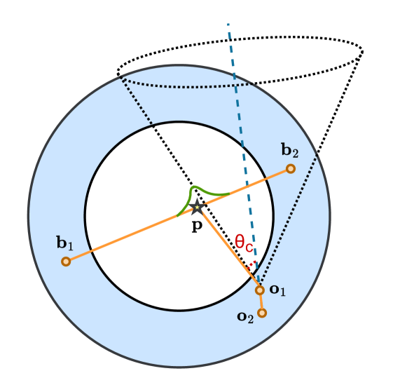
Figure 1: Estimating the point of emission using Compton kinematics. $\bm{b}_{1}$ and $\bm{b}_{2}$ respectively the first and second photon detected positions resulting from the annihilation (back-to-back photons) while $\bm{o}_{1}$ and $\bm{o}_{2}$ are respectively the first and second interaction positions of the prompt gamma in the detector. The yellow star indicates the real emission point.

Two different detector systems have been developed over the past two decades for the implementation of such 3g PET imaging systems. The first one concerns the development of a LXe Compton camera (e.g., the XEMIS project [4]) where the LXe acts as the scatterer and detection medium for the third photon but also for the two annihilation 511keV photons [5]. The second one involves the utilization of a dual-detector structure combining PET and Compton imaging, with the second detector acting as the scatterer [3, 6]. However, these systems do not determine the order of the interactions in the detector.

Recent advancements in 3g imaging reconstruction techniques have aimed to enhance image quality while utilizing low statistics. [7] [7] introduced a method that uses the intersection point of the Compton cone and two coincidence photons of the LOR as the center for a PDF, similar to TOF PET. [8] [8] proposed a scanner design with separate scatterer and absorber modules, incorporating scatter angle calculations using the KN formula and modeling blurring with asymmetric Gaussian functions. Both approaches rely on identifying the LOR-Compton cone intersection point, but face challenges in determining the order of prompt gamma interactions. Yoshida’s scatter-absorber design addresses this through hardware modifications and energy windowing, albeit at the cost of reduced sensitivity. In contrast, the XEMIS-like scanner uses a single dense ring of LXe, where prompt gammas interact multiple times until absorption. This design, while promising, lacks a built-in mechanism for determining interaction order and is susceptible to errors from spatial resolution limitations and Doppler effects, especially given the proximity of interaction points.

Our proposed method, Direct3$\bm{\gamma}$PET, presents a structured pipeline for reconstructing 3D 3g PET images on an event-by-event basis. This approach consists of three main stages, as illustrated in Figure 2:

1. Event Detection and Compton Cone Construction: We start by detecting raw 3g events from the scanner data. Next, we use a GNN-based architecture, called MIN, to sequence the interactions of photons. Finally, we construct the Compton cone based on first and second interactions.

2. LOR processing and histo-image generation: this stage incorporates blurring effects on the LOR using the DREP method, accounts for detection system uncertainties, applies attenuation correction, and generates a histo-image as a preliminary representation of the activity distribution.

3. Image Reconstruction and Enhancement: the final stage employs an encoder-Decoder CNN for image processing, performing both deblurring and denoising to enhance image quality.

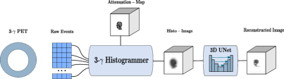
Figure 2: Direct-3$\gamma$ pipeline, from event detection, building histo-image using the histogrammer and the backbone to reconstruct the final image.

Various approaches have been proposed to address the challenges in stage (i). [9] [9] presented an algorithm to reconstruct Compton scattering sequences by minimizing a $\mathrm{d}\phi$-criterion among $N!$ possible sequences. [10] [10] introduced a Bayesian approach utilizing additional information about photon interactions and detector characteristics. While effective, these methods are computationally expensive. [11] [11] developed a NN to improve efficiency, but it remains limited for complex scenarios ($N>4$). To overcome these limitations, we propose two novel approaches. Firstly, a GNN inspired by [12] [12], using a modified IN to classify edges and determine the prompt gamma’s path in the detector. Secondly, we introduce an order-less approach that estimates intersection points using all potential sequences, addressing accuracy issues in complex scenarios.

For stage (ii), we build upon previous work in incorporating detector uncertainties. [7] [7] propagated spatial and energy uncertainties to angle uncertainties, modeling them as symmetric Gaussians on the LOR. [8] [8] proposed the use of a non-symmetric Gaussian and noted that the position estimations are highly accurate when this angle is close to 90^o. However, as the angle approaches 0^o, the accuracy diminishes significantly, resulting in increased background noise when such positions are back-projected with the same intensity. They introduced a DRF model specifically designed to incorporate the blurring effects along the LOR that arise from energy resolution discrepancies. Our DREP module extends these concepts, propagating energy resolution (modeled as a Gaussian distribution with 9% FWHM for 511-keV photons in XEMIS) and spatial uncertainties (uniform distribution within 3.125 mm³ voxels) to estimate Compton angle uncertainty. We then construct the histo-image by back-projecting the estimated asymmetric Gaussians.

For stage (iii), we employ a 3D model capable of doing image to image translation mapping histo-images to real emission sites in approximately real time.

This paper is structured as follows: Section II details the complete pipeline from raw data to reconstructed images. Section III presents the results of reconstructed images using different versions of the pipeline. Section IV discusses limitations, potential improvements and alternative approaches. Finally, Section V concludes this paper.

II Method

The objective is to reconstruct an activity 3D image $\bm{x}\in\mathbb{R}^{P}$ where $P$ is the number of voxels in the FOV, from a collection of $K$ 3g detection events.

II-A Photon Interaction Sequence Determination

In this section we describe our approach to determine the photon interaction sequence determination, which is then used to draw the Compton cone. While the standard approach consists in considering events with two interactions only (which represents $\approx 30$% of the events) and assuming that the interaction with the largest energy deposit is the first (which is not guaranteed), our approach is designed to process events with more than two interactions.

A prompt gamma detection event is represented by a collection of $N$ events (in unknown order), $\bm{o}_{1}=(\bm{r}_{1},E_{1}),\dots,\bm{o}_{N}=(\bm{r}_{N},E_{N})$ where for all $k=1,\dots,N$, $\bm{r}_{k}=(x_{k},y_{k},z_{k})\in\mathbb{R}^{3}$ is the 3D location of the $k$th interaction and $E_{k}$, $k\geq 1$ is the deposited energy at the $k$th interaction. In addition to the prompt gamma, two bact-to-back 511-keV gamma rays are emitted and are detected at $\bm{b}_{1}$ and $\bm{b}_{2}$ (see Figure 1).

Considering that a prompt gamma interacts $N$ times in the detector, i.e., $N-1$ Compton scatters interactions followed by a final photo-absorption, there are $N!$ possible paths. We first describe the $\mathrm{d}\phi$-criterion approach (Section II-A1) and a conventional NN approach from the literature (Section II-A2). We then, introduce our proposed MIN (Section II-A3).

II-A1 The $\mathbf{d}\bm{\phi}$-criterion

In Compton kinematics, the relationship between the $k$th scattering angle $\theta_{k}^{\mathrm{kin}}$, $k=1,\dots N-2$ ($N$ points define $N-2$ angles) and the deposited energy is given by the Compton scattering equation, i.e.,

$$\cos\theta^{\mathrm{kin}}_{k}=1-\frac{m_{\mathrm{e}}c^{2}E_{k+1}}{E_{k}(E_{k}-E_{k+1})}$$

where is $m_{\mathrm{e}}$ is the mass of an electron and $c$ is the speed of light. The $\mathrm{d}\phi$-criterion [9] evaluates the fit between the geometric angles $\theta^{\mathrm{geom}}_{k}$ (determined by a given sequence of interactions) and $\theta^{\mathrm{kin}}_{k}$, $k=1,\dots,N-2$, as

$$\mathrm{d}\phi=\sum_{k=1}^{N-2}\left(\cos\theta^{\mathrm{kin}}_{k}-\cos\theta^{\mathrm{geom}}_{k}\right)^{2}\,.$$ (1)

The photon interaction sequence is determined by minimizing (1), which is achieved by computing all possible sequences. Note that the solution is not necessarily unique.

II-A2 Fully-Connected Neural Network

Multi-layer feed-forward NN are universal function approximators. [11] [11] proposed an architecture that takes as input the normalized deposited energy and positions of interactions with other statistics obtained via simulation such as the Compton scatter angle, the measured total energy, the $\mathrm{d}\phi$-criterion, the distance between the interactions, as well as the absorption and scatter probabilities and the number of interactions. The FCNN contains one hidden layer whose task is to classify the right sequence, such that the output layer contains $N!$ neurons, each of which referring to a possible path with a given probability—the path with highest probability in then chosen. [11] showed that this type of network is suitable for events with $N=3$ or $4$ interactions but may diverge with for $N>4$ due to the complexity.

We implemented a modified version of the architecture proposed by [11] (Figure 3) with deeper layers and which is trained on deposited energy and position coordinates only, without providing additional information about other statistics. This simplified architecture is easier to train and will be used for comparison (Section III-A).

Figure 3: FCNN architectures for photon path estimation: where $x_{i},y_{i},z_{i}$ are the normalized coordinates of each hit, $E_{i}$ the deposited energy,

II-A3 Modified Interaction Network for Sequence Reconstruction (Proposed Method)

In their original paper, [13] [13] proposed an architecture, namely IN, which takes a directed graph as input an outputs values associated to the nodes, edges or the entire graph (e.g., graph classification). The method proved to be a powerful general framework for modeling objects and relations between them.

[12] [12] proposed a GNN framework for gamma-ray track reconstruction in germanium detector arrays. The position of the interaction source is known, and the network is tasked with determining the positions and energies of gamma interactions within the detector. The network must also disentangle and build separate tracks for different gamma photons that are emitted simultaneously, ensuring accurate reconstruction even in complex scenarios with multiple interactions. In our case the initial emission is unknown: only $N$ interactions of a single photon that arrives on a region of a detector is known. We propose a simple GNN architecture using the framework proposed in [13].

We consider a collection of $N$ nodes $\bm{o}_{1},\dots,\bm{o}_{N}$, with $N_{\mathrm{f}}$ features, i.e, for all $k=1,\dots,N$, $\bm{o}_{k}\in\mathbb{R}^{N_{\mathrm{f}}}$, and $N_{\mathrm{e}}=N(N-1)$ possible edges. The nodes are concatenated in a matrix $\bm{O}=[\bm{o}_{1}^{\top},\dots,\bm{o}_{N}^{\top}]^{\top}\in\mathbb{R}^{N\times N_{\mathrm{f}}}$ where ‘^⊤’ denotes the matrix transposition. In our case, $\bm{o}_{k}=(\bm{r}_{k},E_{k})$ and the number of features per node is $N_{\mathrm{f}}=4$. We propose a method based on IN to determine photon interaction sequences from $\bm{O}$. This approach treats the problem as an edge classification task on a graph-structured representation of the interactions. Note that for the purpose of Compton cone determination, only the two first interactions need to be determined.

In [13] the graph is built using two separate matrices that define how messages are passed between nodes. The sender and receiver matrices, respectfully denoted $\bm{R}_{\mathrm{s}}\in\mathbb{R}^{N\times N_{\mathrm{e}}}$ and $\bm{R}_{\mathrm{r}}\in\mathbb{R}^{N\times N_{\mathrm{e}}}$, are defined as

$$[\bm{R}_{\mathrm{s}}]_{n,l}=\left\{\begin{array}[]{ll}1&\text{if edge $l$ departs from node $n$}\\ 0&\text{otherwise}\end{array}\right.$$

and

$$[\bm{R}_{\mathrm{r}}]_{n,l}=\left\{\begin{array}[]{ll}1&\text{if edge $l$ arrives at node $n$}\\ 0&\text{otherwise}\end{array}\right.\,$$

For example the sender and receiver matrices corresponding to the graph in Figure 4(a) are

$$\bm{R}_{\mathrm{s}}=\hbox{}\vbox{\kern 0.86108pt\hbox{$\kern 0.0pt\kern 2.5pt\kern-2.5pt\left[\kern 0.0pt\kern-2.5pt\kern-5.55557pt\vbox{\kern-0.86108pt\vbox{\vbox{ \halign{\kern\arraycolsep\hfil\@arstrut$\kbcolstyle#$\hfil\kern\arraycolsep& \kern\arraycolsep\hfil$\@kbrowstyle#$\ifkbalignright\relax\else\hfil\fi\kern\arraycolsep&& \kern\arraycolsep\hfil$\@kbrowstyle#$\ifkbalignright\relax\else\hfil\fi\kern\arraycolsep\cr 2.5pt\hfil\@arstrut$\scriptstyle$\hfil\kern 2.5pt&2.5pt\hfil$\scriptstyle\bm{e}_{1}$\hfil\kern 2.5pt&2.5pt\hfil$\scriptstyle\bm{e}_{2}$\hfil\kern 2.5pt&2.5pt\hfil$\scriptstyle\bm{e}_{3}$\hfil\kern 2.5pt&2.5pt\hfil$\scriptstyle\bm{e}_{4}$\hfil\kern 2.5pt&2.5pt\hfil$\scriptstyle\bm{e}_{5}$\hfil\kern 2.5pt&2.5pt\hfil$\scriptstyle\bm{e}_{6}\\\bm{o}_{1}$\hfil\kern 2.5pt&2.5pt\hfil$\scriptstyle 1$\hfil\kern 2.5pt&2.5pt\hfil$\scriptstyle 0$\hfil\kern 2.5pt&2.5pt\hfil$\scriptstyle 1$\hfil\kern 2.5pt&2.5pt\hfil$\scriptstyle 0$\hfil\kern 2.5pt&2.5pt\hfil$\scriptstyle 0$\hfil\kern 2.5pt&2.5pt\hfil$\scriptstyle 0\\\bm{o}_{2}$\hfil\kern 2.5pt&2.5pt\hfil$\scriptstyle 0$\hfil\kern 2.5pt&2.5pt\hfil$\scriptstyle 1$\hfil\kern 2.5pt&2.5pt\hfil$\scriptstyle 0$\hfil\kern 2.5pt&2.5pt\hfil$\scriptstyle 0$\hfil\kern 2.5pt&2.5pt\hfil$\scriptstyle 1$\hfil\kern 2.5pt&2.5pt\hfil$\scriptstyle 0\\\bm{o}_{3}$\hfil\kern 2.5pt&2.5pt\hfil$\scriptstyle 0$\hfil\kern 2.5pt&2.5pt\hfil$\scriptstyle 0$\hfil\kern 2.5pt&2.5pt\hfil$\scriptstyle 0$\hfil\kern 2.5pt&2.5pt\hfil$\scriptstyle 1$\hfil\kern 2.5pt&2.5pt\hfil$\scriptstyle 0$\hfil\kern 2.5pt&2.5pt\hfil$\scriptstyle 1$\hfil\kern 2.5pt\crcr}}}}\right]$}}$$

and

$$\bm{R}_{\mathrm{r}}=\hbox{}\vbox{\kern 0.86108pt\hbox{$\kern 0.0pt\kern 2.5pt\kern-2.5pt\left[\kern 0.0pt\kern-2.5pt\kern-5.55557pt\vbox{\kern-0.86108pt\vbox{\vbox{ \halign{\kern\arraycolsep\hfil\@arstrut$\kbcolstyle#$\hfil\kern\arraycolsep& \kern\arraycolsep\hfil$\@kbrowstyle#$\ifkbalignright\relax\else\hfil\fi\kern\arraycolsep&& \kern\arraycolsep\hfil$\@kbrowstyle#$\ifkbalignright\relax\else\hfil\fi\kern\arraycolsep\cr 2.5pt\hfil\@arstrut$\scriptstyle$\hfil\kern 2.5pt&2.5pt\hfil$\scriptstyle\bm{e}_{1}$\hfil\kern 2.5pt&2.5pt\hfil$\scriptstyle\bm{e}_{2}$\hfil\kern 2.5pt&2.5pt\hfil$\scriptstyle\bm{e}_{3}$\hfil\kern 2.5pt&2.5pt\hfil$\scriptstyle\bm{e}_{4}$\hfil\kern 2.5pt&2.5pt\hfil$\scriptstyle\bm{e}_{5}$\hfil\kern 2.5pt&2.5pt\hfil$\scriptstyle\bm{e}_{6}\\\bm{o}_{1}$\hfil\kern 2.5pt&2.5pt\hfil$\scriptstyle 0$\hfil\kern 2.5pt&2.5pt\hfil$\scriptstyle 1$\hfil\kern 2.5pt&2.5pt\hfil$\scriptstyle 0$\hfil\kern 2.5pt&2.5pt\hfil$\scriptstyle 1$\hfil\kern 2.5pt&2.5pt\hfil$\scriptstyle 0$\hfil\kern 2.5pt&2.5pt\hfil$\scriptstyle 0\\\bm{o}_{2}$\hfil\kern 2.5pt&2.5pt\hfil$\scriptstyle 1$\hfil\kern 2.5pt&2.5pt\hfil$\scriptstyle 0$\hfil\kern 2.5pt&2.5pt\hfil$\scriptstyle 0$\hfil\kern 2.5pt&2.5pt\hfil$\scriptstyle 0$\hfil\kern 2.5pt&2.5pt\hfil$\scriptstyle 0$\hfil\kern 2.5pt&2.5pt\hfil$\scriptstyle 1\\\bm{o}_{3}$\hfil\kern 2.5pt&2.5pt\hfil$\scriptstyle 0$\hfil\kern 2.5pt&2.5pt\hfil$\scriptstyle 0$\hfil\kern 2.5pt&2.5pt\hfil$\scriptstyle 1$\hfil\kern 2.5pt&2.5pt\hfil$\scriptstyle 0$\hfil\kern 2.5pt&2.5pt\hfil$\scriptstyle 1$\hfil\kern 2.5pt&2.5pt\hfil$\scriptstyle 0$\hfil\kern 2.5pt\crcr}}}}\right]$}}$$

which should be read for example (first column of $\bm{R}_{\mathrm{s}}$ and $\bm{R}_{\mathrm{e}}$) as “$\bm{e}_{1}$ sends information from $\bm{o}_{1}$ to $\bm{o}_{2}$”.

(a) Input graph

(b) Possible output graph

Figure 4: 4(a) Fully connected graph used as an input for the GNN; 4(b) possible output of the GNN.

The first step in the design of an IN is to create a message matrix $\bm{M}$ defined as

$$\bm{M}=[\bm{R}_{\mathrm{s}}^{\top}\bm{O},\bm{R}_{\mathrm{r}}^{\top}\bm{O}]\in\mathbb{R}^{N_{\mathrm{e}}\times 2N_{\mathrm{f}}}\,.$$

where $[\cdot,\cdot]$ denotes the horizontal concatenation of two matrices with the same number of rows, the total number of directed edges is $N_{\mathrm{e}}=N(N-1)$. Each row in $\bm{M}$ corresponds to an edge and contains $2N_{\mathrm{f}}$ features.

In a second step we encode the information carried in each edge into an effect vector of dimension $N_{\mathrm{eff}}$ via a NN $f_{\mathrm{R}}:\mathbb{R}^{2N_{\mathrm{f}}}\mapsto\mathbb{R}^{N_{\mathrm{eff}}}$ (we used $N_{\mathrm{eff}}=50$ as suggested in [13] [13]) which maps each row of $\bm{M}$ to an $N_{\mathrm{eff}}$-dimensional row vector (In the original paper [13] [13] $f_{\mathrm{R}}$ is refereed to as as a relation-centric network as it operates on edges and encodes relations values).

By repeating the operation on each row, $f_{\mathrm{R}}$ maps $\bm{M}$ to an $N_{\mathrm{e}}\times N_{\mathrm{eff}}$ matrix denoted $\bm{E}$ referred to as the effect matrix. Each row in $\bm{E}$ represents a latent vector of effect for each node on its neighbor.

In a third step the cumulative effect of interactions received by each node is stored in a $N\times N_{\mathrm{eff}}$ matrix $\bar{\bm{E}}$ defined as

$$\bar{\bm{E}}=\bm{R}_{\mathrm{r}}\bm{E}\,,$$

and we define the $N\times(N_{\mathrm{f}}+N_{\mathrm{eff}})$ matrix

$$\bm{C}=[\bm{O},\bar{\bm{E}}]\,.$$

Each row in $\bm{C}$ contains the node’s features combined with the interaction effects. An object-centric function $f_{\mathrm{O}}$ maps the $N_{\mathrm{f}}+N_{\mathrm{eff}}$ features for each of the $N$ nodes to a 10-dimensional vector, resulting in a $N\times 10$ matrix which is then flattened into a $10N$-dimensional column vector. We used an edge model $f_{\mathrm{E}}\colon\mathbb{R}^{10N}\to\mathbb{R}^{N_{\mathrm{e}}}$ which maps the new node features vector to a vector of $N_{\mathrm{e}}$ weights, each weight corresponding to an edge. We used sigmoid activation function in order to give a score between 0 and 1 for each edge.

The overall procedure (Figure 5) defines a mapping $\bm{F}_{\bm{\vartheta}}\colon\mathbb{R}^{N\times N_{\mathrm{f}}}\to[0,1]^{N_{\mathrm{e}}}$ where the parameter $\bm{\vartheta}$ encompasses those of $f_{\mathrm{R}}$, $f_{\mathrm{O}}$ and $f_{\mathrm{E}}$, which maps a sequence of interactions $(\bm{r}_{1},E_{1}),\dots,(\bm{r}_{N},E_{N})$ to a $N_{\mathrm{e}}$-dimensional fuzzy vector containing scores for each edge. Edges with a score lower than 0.5 are then removed, which returns the final graph (Figure 4(b) shows a possible output). This representation allows the model to learn complex patterns of energy deposits and scattering angles without explicitly encoding physics rules [12]. GNN can process variable numbers of interaction points per event. This approach also scales well to large numbers of interaction points better than the FCNN.

Note that $\bm{F}_{\bm{\vartheta}}$ does not discard non-admissible graphs, that is to say, containing V-structures (two edges departing from one node or two edges pointing to one node) and cycles. However, as we will see in Section III-A, a well-trained network is unlikely to return such graphs. In addition, the architecture of $\bm{F}_{\bm{\vartheta}}$ does not guarantee that two permutation-equivariant collections of nodes $\bm{O}$ and $\bm{O}^{\prime}$ are mapped to the same graph. We will also show in Section III-A that the same graphs (after binarisation) are obtained in most cases.

The model is trained from a collection of interaction/graph pairs $(\bm{O},\bm{y})$, $\bm{y}\in\{0,1\}^{N_{\mathrm{e}}}$ being a binary vector corresponding to the true sequence of interaction such that $[\bm{y}]_{\ell}=1$ if the edge $\bm{y}_{\ell}$ is present and $[\bm{y}]_{\ell}=0$ otherwise (for example in Figure 4(b) the graph corresponds to $\bm{y}=[0,0,1,0,0,1]^{\top}$), obtained from MC simulations, by minimizing the cross-entropy between the estimated (fuzzy) graph $\bm{F}_{\bm{\vartheta}}(\bm{O})$ and $\bm{y}$

$$\min_{\bm{\vartheta}}\, \mathbb{E}_{(\bm{O},\bm{y})}[\mathcal{L}(\bm{F}_{\bm{\vartheta}}(\bm{O}),\bm{y})]\,,$$

$$\mathcal{L}(\bm{z},\bm{y})\triangleq -\sum_{l=1}^{N_{\mathrm{e}}}y_{l}\log z_{l}+(1-y_{l})\log(1-z_{l})\,\forall\bm{y},\bm{z}\in\mathbb{R}^{N_{\mathrm{e}}}\,.$$

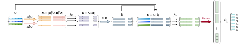
Figure 5: MIN—Proposed architecture for $\bm{F}_{\bm{\vartheta}}$ used to classify edges or relations between photons interactions in the detector.

II-B Histo-image Generation

II-B1 Emission Point Estimation

Using the first two interaction positions $\bm{r}_{1}$ and $\bm{r}_{2}$, the initial energy $E_{\rm{init}}=1.157\ \text{MeV}$ and $E_{1}$ is the deposited energy in the first interaction, the Compton cone can be determined. The cone’s angle $\theta_{\mathrm{c}}\in[-\pi/2,\pi/2]$ is calculated using the KN formula:

$$\cos(\theta_{\mathrm{c}})=1-\frac{m_{\mathrm{e}}c^{2}E_{1}}{E_{\rm{init}}(E_{\rm{init}}-E_{1})}$$ (2)

The cone’s vertex is positioned at the first interaction point of the photon, and its axis runs through to the second interaction point (Figure 1).

The emission point of a prompt gamma can be estimated as the intersection point $\bm{p}\in\mathbb{R}^{3}$ between the Compton cone and the LOR given by the two points $\bm{b}_{1}$ and $\bm{b}_{2}$, i.e., by solving

$$\frac{(\bm{p}-\bm{r}_{1})\cdot\bm{n}}{\|\bm{p}-\bm{r}_{1}\|_{2}}=\cos(\theta_{c}).$$

where $\bm{n}$ is the directional (unitary) vector from $\bm{o}_{2}$ to $\bm{o}_{1}$.

II-B2 Modeling Spatial Uncertainty

However, practical implementation of this method faces challenges due to detector imperfections. In the case of the XEMIS-2 detector, significant uncertainties exist in both energy and spatial measurements. The detector exhibits an energy resolution of 9% FWHM for 511 keV $\gamma$-rays, modeled as a Gaussian distribution around measured energy values. The intrinsic spatial resolution is determined by the detector size and assumed to follow a uniform distribution.

Translating the uncertainties associated with the detector’s measurements to the cone angle $\theta_{\mathrm{c}}$ results in uncertainty around the estimated point $\bm{p}$ on the LOR. However, using a symmetric error model around the estimated point, as described in [7] [7], is not the most effective method for projecting this error from the Compton cone to the LOR. The uncertainty along the LOR is influenced by several factors, including the crossing angle between the Compton cone and the LOR as well as the distance between the vertex of the cone and the LOR. Drawing inspiration from the findings in [8] [8], we propose applying a non-symmetric Gaussian distribution around the estimated point.

Our model uses the the $\sigma^{+}_{\mathrm{mix}}$ and $\sigma^{-}_{\mathrm{mix}}$ STD calculated by DREP (in Appendix, Equation (4) and Equation (5)) to define a collection of “histo-functions” $h_{\bm{p}}$ for all of the $K$ events. The mathematical formulation is:

$$h_{\bm{p}}(t)=\begin{cases}\frac{1}{\sqrt{2\pi(\sigma^{+}_{\mathrm{mix}}+\sigma^{-}_{\mathrm{mix}})}}\exp\left(-\frac{(t-t_{0})^{2}}{2(\sigma^{-}_{\mathrm{mix}})^{2}}\right)&\text{for }t<t_{0},\\ \frac{1}{\sqrt{2\pi(\sigma^{+}_{\mathrm{mix}}+\sigma^{-}_{\mathrm{mix}})}}\exp\left(-\frac{(t-t_{0})^{2}}{2(\sigma^{+}_{\mathrm{mix}})^{2}}\right)&\text{for }t\geq t_{0}.\end{cases}$$ (3)

where $t_{0}$ is the position of $\bm{p}$ along the LOR defined by $\bm{b}_{1}$ and $\bm{b}_{2}$

II-B3 Three-gamma Histogrammer

We define a 3g histogrammer using a non-symmetric Gaussian PDF to model emission event distribution along the LOR. This approach extends the Most Likely Annihilation Position histogrammer proposed by [14] [14] for TOF PET.

The 3g histo-image is created by summing voxelized $P$-dimensional versions of the $h_{\bm{p}}(t)$ for each estimated location $\bm{p}$, $P$ being the number of voxels, resulting in a $P$-dimensional radioactivity image.

II-B4 Attenuation Correction

In 3g PET imaging with ⁴⁴Sc, we need to correct for attenuation of 511 keV and 1,157 keV gamma rays. The attenuation correction factors $a_{\bm{p}}$ for each $\bm{p}$ is given by

$$a_{\bm{p}}=\mathrm{e}^{\int_{\bm{b}_{1}}^{\bm{b}_{2}}\mu_{511}(\bm{r})\,\mathrm{d}{}\bm{r}}\cdot\mathrm{e}^{\int_{\bm{p}}^{\bm{o}_{1}}\mu_{1157}(\bm{r})\,\mathrm{d}{}\bm{r}}$$

where $\mu_{511}(\bm{r})$ and $\mu_{1157}(\bm{r})$ are the attenuation coefficients at position $\bm{r}\in\mathbb{R}^{3}$ for 511 keV and 1,157 keV gamma rays, respectively. The attenuation-corrected histo-function is

$$h_{\bm{p}}^{\mathrm{att}}(x)=a_{\bm{p}}\cdot h_{\bm{p}}(t)\,$$

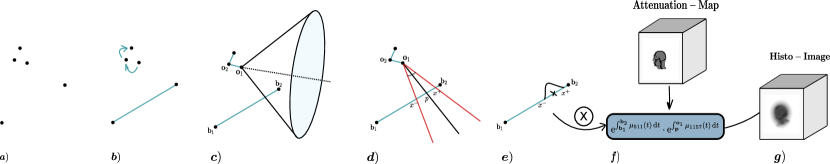
Figure 6: Workflow of the DIRECT-3$\gamma$ Histogrammer: (a) detection of hits by the 3g PET scanner; (b) construction of LOR and determination of prompt gamma interaction order; (c) estimation of intersection between Compton cone and LOR; (d) calculation of uncertainties on the LOR; (e) projection of estimated Gaussian distribution onto image space; and (f) application of attenuation correction.

II-C From the Histo-image to the Final Image

Equation (II-B1) can result in two possible intersection points between the Compton cone and the LOR within the FOV. Both of these solutions are utilized in the creation of histo-images, which leads to noise caused by false positives in the image. Another possible source of noise is inaccuracies in the algorithm that is responsible for determining the sequence of detected gamma rays. Furthermore, we need to correct for the uncertainty along the LOR in the histo-images. Additionally, PR should also be corrected for, although we did not implement it in this work.

To address the issue of blurring and noise in histo-images, we propose the use of an attention U-Net model [15] as the backbone for our image-to-image translation tasks (the full pipeline is illustrated in Figure 2). In this work, we trained and compared two different models: a supervised model, Direct3$\bm{\gamma}$PET_S and a generative model Direct3$\bm{\gamma}$PET_G. The Attention U-Net introduces novel AG which enhance the model’s ability to focus on relevant regions of the input images while suppressing irrelevant information. This mechanism is particularly effective for tasks involving complex anatomical structures, ensuring high sensitivity and accuracy in predictions.

For the supervised model Direct3$\bm{\gamma}$PET_S, we utilize the attention U-Net $\bm{G}_{\bm{\psi}}\colon\mathbb{R}^{P}\to\mathbb{R}^{P}$ with parameter $\bm{\psi}$ to map histo-images $\bm{x}\in\mathbb{R}^{P}$ to true emission point images $\bm{x}^{\star}\in\mathbb{R}^{P}$, as demonstrated in [14] [14]. The training is achieved by minimizing a $L^{1}$ loss function. The extended model Direct3$\bm{\gamma}$PET_G incorporates a patch discriminator and a LS GAN loss functions (i.e., with a discriminator loss) as proposed by [16] [16] and [17] [17].

II-D Detector Setup and Dataset

II-D1 Detector

Data was acquired using simulations on GATE [18] with a human-sized scanner similar in dimensions to the Siemens mMR. This scanner featured an inner diameter of 60 cm and an outer diameter of 90 cm. The detector was modified to use LXe as in the XEMIS scanner. The pixel size was set to $3.125\times 3.125$ mm², with a longitudinal spatial resolution of less than $100$ µm. The energy resolution was approximately $9\%$ FWHM at 511 keV, matching the specifications of the XEMIS2 scanner [19, 20, 21].

II-D2 Training and Evaluation Datasets

Experiment 1

To train MIN and the FCNN, we conducted a simulation using a uniform cylinder in the FOV. This simulation produced up to 20 million 3g events. We only included events where all gamma rays fully interacted with the detector, meaning the sum of deposited energies across all interactions equaled 1.157 MeV. We created different MIN and FCNN based on the number of interactions in each event. For testing, we used a separate dataset of 2 million events, also generated from a uniform cylinder in the FOV.

Experiment 2 and 3: Training of Direct3$\bm{\gamma}$PET_S and Direct3$\bm{\gamma}$PET_G

A variety of 200 XCAT ⁴⁴Sc activity and attenuation (511 keV for back-2-back gammas and 1.157 MeV for the prompt gamma) phantoms [22] ($200\times 200\times 200$, $3$ mm³ voxel size) were utilized, encompassing different anatomical size, shapes and regions. Spherical lesions of varying shapes were randomly added to different regions of these phantoms to simulate diverse scenarios. For each phantom, 1 to 20 Millions 3g events were generated.

We produced histo-images using our histogrammer (Section II-B3), where the Compton cones were determined using three different approaches: (i) by determining the interaction sequences using MIN (Section II-A), namely HO, (ii) by only considering events with exactly two interactions of the prompt gamma, namely H2P, and (iii) by drawing all possibles Compton cones from all possible interaction sequences (thus resulting in a very noisy histo-image representing the worst case scenario), namely HMC. Direct3$\bm{\gamma}$PET_S and Direct3$\bm{\gamma}$PET_G were then trained to map the histo-images $\bm{x}$ to their corresponding GT images $\bm{x}^{\star}$ as described in Section II-C.

To enhance model robustness and prevent overfitting, we implemented a comprehensive data augmentation process during training using various random rigid transformations such as flipping, rotations, translations, with additional intensity rescaling.

The evaluation was conducted using 5 different XCAT volumes, each generated separately with varying body positions and activities. These phantoms are illustrated in Figure 7, which shows transverse emission images for each of the five phantoms used in the study.

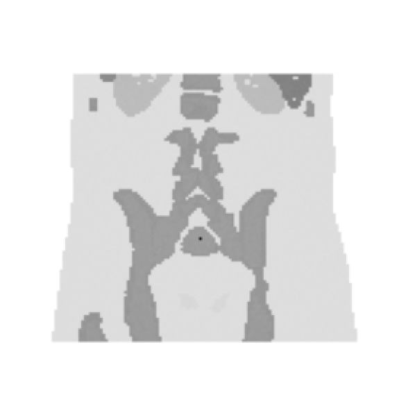
(a) Phantom 1

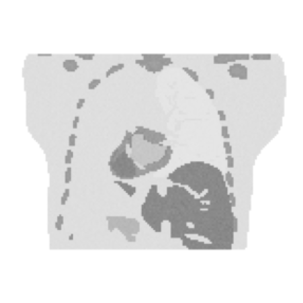
(b) Phantom 2

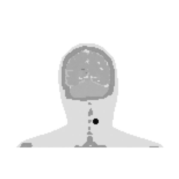
(c) Phantom 3

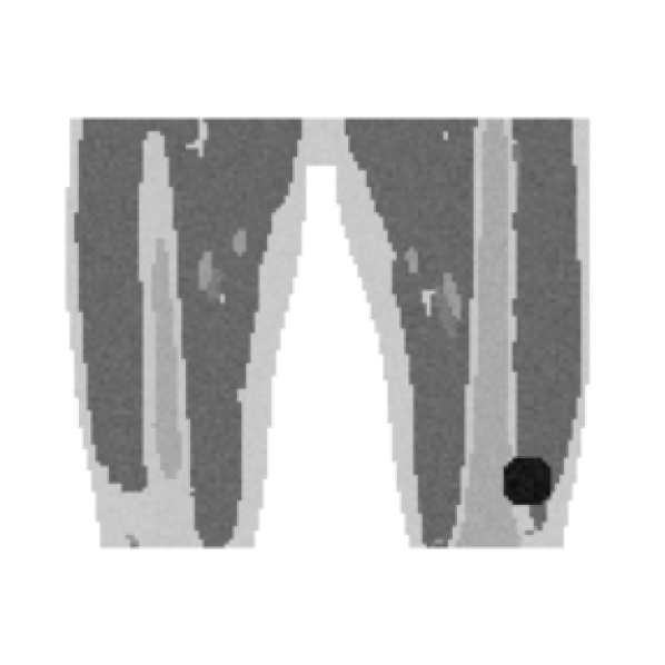
(d) Phantom 4

(e) Phantom 5

Figure 7: Coronal views of the Phantoms used in test dataset.

III Results

III-A Experiment 1: Photon Interaction Sequence Determination

In this section we show the results on prediction of the order of interaction of the three methods described in Section II-A, i.e., $\mathrm{d}\phi$-criterion, FCNN and MIN (proposed approach), from the simulated data (Section II-D2).

Table I presents the accuracy of the three algorithms in predicting photon interaction sequences. The table shows results for events with 3, 4, and 5 interactions. For events with only 2 interactions, no algorithm was applied; instead, we simply chose the position with the highest energy as the first interaction, resulting in approximately 81% accuracy. The table includes two additional columns: “All Events” and “First 2 only”. The “All Events” column represents the overall accuracy of reconstructing the entire interaction path for all events. The “First 2 only” column shows the accuracy of reconstructing just the first and second points of the sequence (needed for drawing the Compton cone). The accuracy is calculated as

$$\textrm{Accuracy}=\frac{\textrm{Number of well classified sequences}}{\textrm{Total number of events}}\,.$$

Approach	N=3	N=4	N=5	All Events	First 2 only
$\mathrm{d}\phi$-criterion	88	73.5	61	0.78	0.798
FCNN	91	82	59	0.80	0.82
MIN	93.5	92	77	0.864	0.877

TABLE I: Experiment 1—Comparison of the three different approaches ($\mathrm{d}\phi$-criterion, FCNN, MIN) for predicting the photon interaction sequence.

The results in Table I demonstrate that the MIN approach consistently outperforms the other two methods across all scenarios. It achieves the highest accuracy for events with 3, 4, and 5 interactions, as well as for overall events and when considering only the first two interactions. As the number of interactions increases, the accuracy of all methods decreases, indicating that longer interaction sequences are more challenging to reconstruct. Interestingly, all methods show slightly higher accuracy when focusing on just the first two interactions, which is crucial for Compton cone reconstruction. It is important to note that MIN produced non-admissible sequences (V-structures, cycles) for 2% of the events, which were included into the accuracy calculations. Despite this limitation, MIN remains the most effective approach for predicting photon interaction sequences in this study.

III-B Experiment 2: Image Reconstruction

In this section, we present a comparative analysis of reconstruction methods using histo-images generated by different ordering algorithms. The histo-images obtained by HO, H2P, and HMC were converted to radioactivity images using Direct3$\bm{\gamma}$PET_S. These images are referred to as OO, O2P and OMC respectively.

Figure 8 shows the histo-images and the resulting radioactivity images for Phantom 1 (Figure 7(a)). From these images, we can see that O2P contains artifacts and lacks homogeneity due to the low number of counts used to build its input H2P (low sensitivity). In contrast, the results from OMC and OO are similar and demonstrate better image quality.

These findings are confirmed quantitatively in Figure 9, which presents a scatter plot of SSIM andPSNR for these methods across multiple patients. The OO method generally outperformed other methods, yielding high SSIM and PSNR values. This suggests that despite not being completely accurate, the ordering algorithm provides reliable reconstruction quality by effectively balancing the trade-off between including more events and maintaining accuracy. Interestingly, the OMC method, which considers all possible interaction orders, showed competitive performance. In some cases, OMC achieved SSIM values comparable to or even slightly higher than OO. This suggests that considering all possible cones can sometimes compensate for the lack of a specific ordering algorithm, potentially due to its ability to capture more information. However, the generally lower PSNR values for OMC indicate that this method may introduce more noise, affecting overall image quality. The O2P method, utilizing only two-interaction events, has the lowest scores. This is likely due to the reduced number of events considered, which lowers the scanner’s sensitivity. While this method ensures that only definite two-interaction events are used, the loss in data quantity significantly impacts reconstruction quality.

GT	H2P	O2P	HMC	OMC	HO	OO

Figure 8: Experiment 2—Outputs of Direct3$\bm{\gamma}$PET_S under different settings. From left to right: GT, H2P, O2P, HMC, OMC, HO, OO.

Figure 9: Scatter plot of SSIM and PSNR values for different reconstruction methods (OO, OMC, and O2P). Each point represents a different patient.

III-C Experiment 3: Direct3$\bm{\gamma}$PET_S vs Direct3$\bm{\gamma}$PET_G

We trained additional model Direct3$\bm{\gamma}$PET_G, independently from scratch for 700 epochs, using HO as input.

Figure 10 includes coronal, sagittal, and transverse views of Phantom 2 (Figure 7(b)). In those images we can see that while Direct3$\bm{\gamma}$PET_S is giving smooth images, it lacking high frequency details, while fine-details are well defined in images resulted by Direct3$\bm{\gamma}$PET_G.

Figure 10 presents coronal, sagittal, and transverse views of the phantom. In these images, while Direct3$\bm{\gamma}$PET_S produces smoother images, it fails to capture high-frequency details. Conversely, Direct3$\bm{\gamma}$PET_G excels in preserving fine details, resulting in more sharply defined and detailed images.

This difference is further illustrated in Figure 11, which presents a scatter plot comparing the performance of Direct3$\bm{\gamma}$PET_S and Direct3$\bm{\gamma}$PET_G in terms of SSIM and PSNR metrics. Direct3$\bm{\gamma}$PET_G achieved higher SSIM values across all tested patients compared to Direct3$\bm{\gamma}$PET_S. However, Direct3$\bm{\gamma}$PET_S exhibited marginally better PSNR performance compared to Direct3$\bm{\gamma}$PET_G.

Several factors contributes to this performance difference: The GAN-based method may excel in preserving structural similarity, which aligns well with the SSIM metric. In contrast, the supervised model’s direct optimization for pixel-wise accuracy contributes to its slightly higher PSNR values. The 3D nature of the reconstruction problem appears to be well-handled by both approaches, with each showing strengths in different aspects of image quality. Despite the small differences, both methods achieve high SSIM and PSNR values, indicating that both approaches are viable for the task. The GAN-based method might offer benefits in terms of structural preservation and perceptual quality.

GT	HO	Direct3$\bm{\gamma}$PETS	rel. difference (Direct3$\bm{\gamma}$PETS)	Direct3$\bm{\gamma}$PETG	rel. difference (Direct3$\bm{\gamma}$PETG)
\begin{overpic}[width=49.86867pt,angle={180},trim=37.13875pt 50.18748pt 37.13875pt 50.18748pt,clip]{images/Expirement3_999/cr_gt_image.pdf} \end{overpic}	\begin{overpic}[width=49.86867pt,angle={180},trim=37.13875pt 50.18748pt 37.13875pt 50.18748pt,clip]{images/Expirement3_999/cr_bp_image.pdf} \end{overpic}	\begin{overpic}[width=49.86867pt,angle={180},trim=37.13875pt 50.18748pt 37.13875pt 50.18748pt,clip]{images/Expirement3_999/cr_sup_image.pdf} \end{overpic}	\begin{overpic}[width=49.86867pt,angle={180},trim=37.13875pt 50.18748pt 37.13875pt 50.18748pt,clip]{images/Expirement3_999/cr_vox2vox_error.pdf} \put(95.0,5.0){\includegraphics[width=7.80748pt,trim=0.0pt 0.0pt 0.0pt 0.0pt,clip]{images/Expirement3_999/Scale_cr.png}} \end{overpic}	\begin{overpic}[width=49.86867pt,angle={180},trim=37.13875pt 50.18748pt 37.13875pt 50.18748pt,clip]{images/Expirement3_999/cr_vox2vox_image.pdf} \end{overpic}	\begin{overpic}[width=49.86867pt,angle={180},trim=37.13875pt 50.18748pt 37.13875pt 50.18748pt,clip]{images/Expirement3_999/cr_vox2vox_error.pdf} \put(95.0,5.0){\includegraphics[width=7.80748pt,trim=0.0pt 0.0pt 0.0pt 0.0pt,clip]{images/Expirement3_999/Scale_cr.png}} \end{overpic}
\begin{overpic}[width=49.86867pt,angle={180},trim=37.13875pt 50.18748pt 37.13875pt 50.18748pt,clip]{images/Expirement3_999/sa_gt_image.pdf} \end{overpic}	\begin{overpic}[width=49.86867pt,angle={180},trim=37.13875pt 50.18748pt 37.13875pt 50.18748pt,clip]{images/Expirement3_999/sa_bp_image.pdf} \end{overpic}	\begin{overpic}[width=49.86867pt,angle={180},trim=37.13875pt 50.18748pt 37.13875pt 50.18748pt,clip]{images/Expirement3_999/sa_sup_image.pdf} \end{overpic}	\begin{overpic}[width=49.86867pt,angle={180},trim=37.13875pt 50.18748pt 37.13875pt 50.18748pt,clip]{images/Expirement3_999/sa_sup_error.pdf} \end{overpic}	\begin{overpic}[width=49.86867pt,angle={180},trim=37.13875pt 50.18748pt 37.13875pt 50.18748pt,clip]{images/Expirement3_999/sa_vox2vox_image.pdf} \end{overpic}	\begin{overpic}[width=49.86867pt,angle={180},trim=37.13875pt 50.18748pt 37.13875pt 50.18748pt,clip]{images/Expirement3_999/sa_vox2vox_error.pdf} \end{overpic}
\begin{overpic}[width=49.86867pt,trim=37.13875pt 50.18748pt 37.13875pt 50.18748pt,clip]{images/Expirement3_999/tr_gt_image.pdf} \end{overpic}	\begin{overpic}[width=49.86867pt,trim=37.13875pt 50.18748pt 37.13875pt 50.18748pt,clip]{images/Expirement3_999/tr_bp_image.pdf} \end{overpic}	\begin{overpic}[width=49.86867pt,trim=37.13875pt 50.18748pt 37.13875pt 50.18748pt,clip]{images/Expirement3_999/tr_sup_image.pdf} \end{overpic}	\begin{overpic}[width=49.86867pt,trim=37.13875pt 50.18748pt 37.13875pt 50.18748pt,clip]{images/Expirement3_999/tr_sup_error.pdf} \end{overpic}	\begin{overpic}[width=49.86867pt,trim=37.13875pt 50.18748pt 37.13875pt 50.18748pt,clip]{images/Expirement3_999/tr_vox2vox_image.pdf} \end{overpic}	\begin{overpic}[width=49.86867pt,trim=37.13875pt 50.18748pt 37.13875pt 50.18748pt,clip]{images/Expirement3_999/tr_vox2vox_error.pdf} \end{overpic}

Figure 10: Experiment 3—Comparison of Direct3$\bm{\gamma}$PET_S and Direct3$\bm{\gamma}$PET_G.

Figure 11: Experiment 2—Scatter plot of SSIM and PSNR values for different reconstruction methods (Direct3$\bm{\gamma}$PET_S and Direct3$\bm{\gamma}$PET_G). Each point represents a different phantom.

IV Discussion

This study introduces a comprehensive approach to 3g PET imaging using ⁴⁴Sc, addressing key challenges in photon interaction sequence determination and emission point estimation. Our proposed MIN demonstrated superior accuracy in determining photon interaction sequences compared to both physical ($\mathrm{d}\phi$-criterion) and classical FCNN methods, particularly when complexity increase and number of interactions of the prompt gamma depass 4. This improvement in sequence determination is crucial for accurate image reconstruction in 3g PET.

We introduced a novel DREP module and implemented a non-symmetric Gaussian function in our 3g histogrammer, both of which have demonstrated significant potential in improving the accuracy of emission event distribution modeling. The DREP module specifically addresses two key types of measurement uncertainties: energy resolution errors and spatial position uncertainties. These uncertainties, inherent in PET detectors, can significantly impact the accuracy of Compton cone reconstruction and, consequently, the precision of emission point estimation. Our 3g histogrammer utilizes this non-symmetric Gaussian approach to more realistically represent the probability distribution of emission points along the LOR. This method accounts for the asymmetric nature of error propagation from the Compton cone to the LOR, a factor often overlooked in conventional symmetric models.

Furthermore, we developed a tailored attenuation correction method specifically for 3g events. Unlike traditional back-to-back annihilation in conventional PET, our method accounts for the attenuation of both the 511 keV annihilation photons and the 1.157 MeV prompt gamma from ⁴⁴Sc decay. This dual-energy attenuation correction is crucial for accurate quantification of activity distribution, especially in larger body regions or dense tissues where attenuation effects are more pronounced. Importantly, we apply this attenuation correction to the histogrammed data before feeding it into our NN for image reconstruction. This pre-processing step is vital as it provides the NN with more accurate input data, allowing it to focus on learning the underlying activity distribution rather than compensating for attenuation effects. By incorporating these physical corrections prior to the deep learning stage, we aim to enhance the overall accuracy and quantitative reliability of the reconstructed PET images.

Our comprehensive analysis of reconstruction methods in 3g imaging has yielded valuable insights into the strengths and limitations of various approaches. Using HO demonstrates superior performance across different scenarios, indicating its effectiveness in optimizing the balance between event inclusion and accuracy. This method’s success can be attributed to its ability to efficiently filter out incorrect interaction sequences while retaining a substantial portion of valid events. Interestingly, using HMC shows competitive performance in certain situations. This approach maximizes information inclusion by backprojecting all potential cones for each event, regardless of the interaction sequence. However, it is important to note that this method comes with significant drawbacks. Firstly, it is computationally intensive, substantially increasing the time required to generate histo-images. For each event, multiple cones must be backprojected, leading to longer processing times. Secondly, this method introduces considerable noise into the histo-images due to the inclusion of incorrect cones, potentially compromising image quality. Despite these limitations, HMC may prove valuable in specific scenarios where reconstruction algorithm development is challenging or not feasible. In such cases, the increased noise and computational cost might be acceptable trade-offs for maximizing data utilization. In contrast, using H2P consistently underperforms compared to the other histo-images. This method, which restricts data selection to events with only two detected interactions, reveals a critical weakness in overly stringent event filtering. While it ensures the use of high-confidence events, it significantly reduces the overall sensitivity of the imaging system. This drastic reduction in usable data compromises the signal-to-noise ratio and, consequently, the overall image quality and quantitative accuracy.

These findings underscore the importance of striking an optimal balance between data inclusion and event confidence in 3g PET imaging. The superior performance of the photon-order algorithm suggests that sophisticated interaction sequence determination methods can significantly enhance image reconstruction quality. However, the potential utility of less restrictive methods in certain scenarios highlights the need for flexible approaches tailored to specific imaging conditions and reconstruction capabilities.

Our comparative analysis of supervised (Direct3$\bm{\gamma}$PET_S) and adversarial (Direct3$\bm{\gamma}$PET_G) training approaches for 3g PET image reconstruction reveals complementary strengths. Direct3$\bm{\gamma}$PET_G generally achieved higher SSIM values, suggesting better structural preservation. Conversely, Direct3$\bm{\gamma}$PET_S showed marginally superior PSNR performance, indicating slightly better noise reduction. These differences likely stem from their distinct optimization objectives: the GAN’s adversarial loss may prioritize structural coherence, while supervised learning directly optimizes pixel-wise accuracy. Importantly, both methods demonstrated high performance across metrics, affirming their viability for 3g PET reconstruction.

V Conclusion

This study introduces and validates a novel approach to 3g-PET imaging using ⁴⁴Sc, addressing key technical challenges and enhancing the accuracy of image reconstruction. Our work demonstrates the efficacy of the MIN method for precise photon interaction sequence determination, significantly outperforming existing techniques. The integration of the DREP and a non-symmetric Gaussian function in the histogrammer has proven crucial in improving the modeling of emission event distributions, thereby refining the overall image quality.

The dual-energy attenuation correction method developed for 3g events, particularly for the 511 keV annihilation photons and the 1,157 keV prompt gamma, ensures more accurate quantification of activity distribution. By applying these corrections before NN processing, we have enhanced the reliability and accuracy of the reconstructed 3g-PET images.

Our comparative analysis of various reconstruction methods underscores the photon-order algorithm’s superior performance in maintaining a balance between data inclusion and accuracy. While more inclusive methods, such as the all-cones approach, offer potential in specific scenarios, their computational demands and noise introduction limit their practicality. Conversely, the restrictive two-interaction method, although precise, compromises overall sensitivity and image quality. Furthermore, the study highlights the advantages of the adversarial approach (Direct3$\bm{\gamma}$PET_G) in preserving structural details and potentially generating more perceptually realistic images, as reflected in its higher SSIM scores.

Future work will focus on adding the attenuation map directely to the network in order to correct attenuation and PR effects directely from an histo-image.

Appendix A Appendix

To address the spatial and energy uncertainties that cause blurring along the LOR in 3g-PET imaging, we have developed a DREP module to determine $\sigma_{\mathrm{mix}}^{\pm}$ in Equation (3). This module accounts for both energy and spatial measurement uncertainties in the estimation of the Compton scattering angle and its propagation to the LOR.

A-A Propagation of Energy Measurement Uncertainty

Given an initial photon energy $E_{\rm{init}}$ and a deposited photon energy $E_{1}$ at first interaction. The Compton scattering equation in terms of the deposited photon energy is given by 2. To find the uncertainty in the scattering angle $\theta_{\mathrm{C}}$ due to the uncertainty in the measured energy, we first take the derivative of $\cos(\theta_{\mathrm{C}})$ with respect to $E_{1}$:

$$\frac{\mathrm{d}(\cos(\theta_{\mathrm{C}}))}{\mathrm{d}E_{1}}=-\frac{m_{\mathrm{e}}c^{2}}{(E_{\rm{init}}-E_{1})^{2}}\,.$$

The uncertainty in $\cos(\theta_{\mathrm{C}})$ is then given by:

$$\Delta\cos(\theta_{\mathrm{C},\mathrm{energy}}) {}=\left|\frac{\mathrm{d}(\cos(\theta_{\mathrm{C}}))}{\mathrm{d}E_{1}}\right|\Delta E_{1}$$

$${}=\left|-\frac{m_{\mathrm{e}}c^{2}}{(E_{\rm{init}}-E_{1})^{2}}\right|\Delta E_{1}\,.$$

Finally, we convert this to the uncertainty in $\theta_{\mathrm{C}}$:

$$\Delta\theta_{\mathrm{C},\mathrm{energy}} {}=\frac{\Delta\cos(\theta_{\mathrm{C},\mathrm{mes}})}{\sin(\theta_{\mathrm{C}})}$$

$${}=\frac{\left|-\frac{m_{\mathrm{e}}c^{2}}{(E_{\rm{init}}-E_{1})^{2}}\right|\Delta E_{1}}{\sin(\theta_{\mathrm{C}})}\,.$$

This equation shows how the error in the measured photon energy propagates to the uncertainty in the scattering angle.

A-B Mixing Energy and Spatial Measurement Uncertainties

In a study on the detector resolution using the XEMIS-1 [21] and XEMIS-2 [23] systems, it was shown that the spatial resolution contribution to the scatter angle error is almost constant and is approximately $\Delta\theta_{\mathrm{C},\mathrm{spatial}}=1.2^{\mathrm{o}}$.

Inspired from [8], we consider variations in the angle $\theta_{\mathrm{C}}$ due to energy and spatial uncertainties:

$$\theta_{\mathrm{C},\text{energy}}^{\pm} =\theta_{\mathrm{C}}\pm\Delta\theta_{\mathrm{C},\text{energy}},\quad\theta_{\mathrm{C},\text{spatial}}^{\pm} =\theta_{\mathrm{C}}\pm\Delta\theta_{\mathrm{C},\text{spatial}}$$

These variations influence the intersection points of the Compton cone with the LOR, resulting in the coordinates $(x_{\text{energy}}^{+},x_{\text{energy}}^{-},x_{\text{spatial}}^{+},x_{\text{spatial}}^{-})$.

We define the blurring on the LOR for each uncertainty as follows:

$$\sigma_{\text{energy}}^{\pm} =\left|x-x_{\text{energy}}^{\pm}\right|,\quad\sigma_{\text{spatial}}^{\pm}=\left|x-x_{\text{spatial}}^{\pm}\right|$$

Finally, we combine these uncertainties using the RSS method, for the positive variation,

$$\sigma_{\text{mix}}^{+}=\sqrt{(\sigma_{\text{energy}}^{+})^{2}+(\sigma_{\text{spatial}}^{+})^{2}}\,,$$ (4)

and the negative variation:

$$\sigma_{\text{mix}}^{-}=\sqrt{(\sigma_{\text{energy}}^{-})^{2}+(\sigma_{\text{spatial}}^{-})^{2}}\,.$$ (5)

References

- [1] JW Kist, B Keizer, M Vlies, AH Brouwers, DA Huysmans, FM Zant, R Hermsen, MP Stokkel, OS Hoekstra and WV Vogel “other members of the THYROPET Study group are John MH de Klerk. 124I PET/CT to predict the outcome of blind 131I treatment in patients with biochemical recurrence of differentiated thyroid cancer; results of a multicenter diagnostic cohort study (THYROPET)” In J Nucl Med 57.5, 2016, pp. 701–7
- [2] Cristina Müller, Maruta Bunka, Josefine Reber, Cindy Fischer, Konstantin Zhernosekov, Andreas Türler and Roger Schibli “Promises of cyclotron-produced 44Sc as a diagnostic match for trivalent –emitters: in vitro and in vivo study of a 44Sc-DOTA-folate conjugate” In Journal of nuclear medicine 54.12 Soc Nuclear Med, 2013, pp. 2168–2174
- [3] P Thirolf, C Lang and K Parodi “Perspectives for Highly-Sensitive PET-Based Medical Imaging Using Coincidences” In Acta Physica Polonica A 127.5 Polska Akademia Nauk. Instytut Fizyki PAN, 2015, pp. 1441–1444
- [4] L Gallego Manzano, S Bassetto, N Beaupere, P Briend, T Carlier, M Cherel, Jean-Pierre Cussonneau, J Donnard, M Gorski and R Hamanishi “XEMIS: A liquid xenon detector for medical imaging” In Nuclear Instruments and Methods in Physics Research Section A: Accelerators, Spectrometers, Detectors and Associated Equipment 787 Elsevier, 2015, pp. 89–93
- [5] L Gallego Manzano, JM Abaline, S Acounis, N Beaupere, JL Beney, J Bert, S Bouvier, P Briend, J Butterworth and T Carlier “XEMIS2: A liquid xenon detector for small animal medical imaging” In Nuclear Instruments and Methods in Physics Research Section A: Accelerators, Spectrometers, Detectors and Associated Equipment 912 Elsevier, 2018, pp. 329–332
- [6] Taiga Yamaya, Eiji Yoshida, Hideaki Tashima, Atsushi Tsuji, Kotaro Nagatsu, Mitsutaka Yamaguchi, Naoki Kawachi, Yusuke Okumura, Mikio Suga and Katia Parodi “Whole gamma imaging (WGI) concept: simulation study of triple-gamma imaging” Soc Nuclear Med, 2017
- [7] D. Giovagnoli, A. Bousse, N. Beaupere, C. Canot, J.-P. Cussonneau, S. Diglio, A. Iborra Carreres, J. Masbou, T. Merlin, E. Morteau, Y. Xing, Y. Zhu, D. Thers and D. Visvikis “A Pseudo-TOF Image Reconstruction Approach for Three-Gamma Small Animal Imaging” In IEEE Transactions on Radiation and Plasma Medical Sciences 5.6, 2021, pp. 826–834 DOI: 10.1109/TRPMS.2020.3046409
- [8] Eiji Yoshida, Hideaki Tashima, Kotaro Nagatsu, Atsushi B Tsuji, Kei Kamada, Katia Parodi and Taiga Yamaya “Whole gamma imaging: a new concept of PET combined with Compton imaging” In Physics in Medicine & Biology 65.12 IOP Publishing, 2020, pp. 125013
- [9] Uwe G Oberlack, Elena Aprile, Alessandro Curioni, Valeri Egorov and Karl-Ludwig Giboni “Compton scattering sequence reconstruction algorithm for the liquid xenon gamma-ray imaging telescope (LXeGRIT)” In Hard X-Ray, Gamma-Ray, and Neutron Detector Physics II 4141, 2000, pp. 168–177 SPIE
- [10] Guillem Pratx and Craig S Levin “Bayesian reconstruction of photon interaction sequences for high-resolution PET detectors” In Physics in Medicine & Biology 54.17 IOP Publishing, 2009, pp. 5073
- [11] Andreas Zoglauer and Steven E. Boggs “Application of neural networks to the identification of the compton interaction sequence in compton imagers” In 2007 IEEE Nuclear Science Symposium Conference Record 6, 2007, pp. 4436–4441 DOI: 10.1109/NSSMIC.2007.4437096
- [12] Mikael Andersson “Gamma-ray racking using graph neural networks”, 2021
- [13] Peter W. Battaglia, Razvan Pascanu, Matthew Lai, Danilo Rezende and Koray Kavukcuoglu “Interaction Networks for Learning about Objects, Relations and Physics”, 2016 eprint: arXiv:1612.00222
- [14] William Whiteley, Vladimir Panin, Chuanyu Zhou, Jorge Cabello, Deepak Bharkhada and Jens Gregor “FastPET: near real-time reconstruction of PET histo-image data using a neural network” In IEEE Transactions on Radiation and Plasma Medical Sciences 5.1 IEEE, 2020, pp. 65–77
- [15] Ozan Oktay, Jo Schlemper, Loic Le Folgoc, Matthew Lee, Mattias Heinrich, Kazunari Misawa, Kensaku Mori, Steven McDonagh, Nils Y Hammerla and Bernhard Kainz “Attention u-net: Learning where to look for the pancreas” In arXiv preprint arXiv:1804.03999, 2018
- [16] Phillip Isola, Jun-Yan Zhu, Tinghui Zhou and Alexei A Efros “Image-to-image translation with conditional adversarial networks” In Proceedings of the IEEE conference on computer vision and pattern recognition, 2017, pp. 1125–1134
- [17] Marco Domenico Cirillo, David Abramian and Anders Eklund “Vox2Vox: 3D-GAN for brain tumour segmentation” In Brainlesion: Glioma, Multiple Sclerosis, Stroke and Traumatic Brain Injuries: 6th International Workshop, BrainLes 2020, Held in Conjunction with MICCAI 2020, Lima, Peru, October 4, 2020, Revised Selected Papers, Part I 6, 2021, pp. 274–284 Springer
- [18] S. Jan, G. Santin, D. Strul, S. Staelens, K. Assie, D. Autret, S. Avner, R. Barbier, M. Bardies, P.. Bloomfield, D. Brasse, V. Breton, P. Bruyndonckx, I. Buvat, A.. Chatziioannou, Y. Choi, Y.. Chung and C. Comtat “GATE: a simulation toolkit for PET and SPECT” In Physics in Medicine & Biology 49.19 IOP Publishing, 2004, pp. 4543
- [19] E Aprile and T Doke “Liquid xenon detectors for particle physics and astrophysics” In Reviews of Modern Physics 82.3 APS, 2010, pp. 2053
- [20] Yuwei Zhu, M Abaline, S Acounis, N Beaupère, JL Beney, J Bert, S Bouvier, P Briend, J Butterworth and T Carlier “Scintillation signal in XEMIS2, a liquid xenon compton camera with 3 imaging technique” In Proceedings of International Conference on Technology and Instrumentation in Particle Physics 2017: Volume 2, 2018, pp. 159–163 Springer
- [21] Lucia Gallego Manzano “Optimization of a single-phase liquid xenon Compton camera for 3 medical imaging”, 2016
- [22] W.. Segars, G. Sturgeon, S. Mendonca, J. Grimes and B… Tsui “4D XCAT phantom for multimodality imaging research” In Medical physics 37.9 Wiley Online Library, 2010, pp. 4902–4915
- [23] Debora Giovagnoli “Image reconstruction for three-gamma PET imaging”, 2020