Polarization of recoil electrons for testing time reversal violation in neutrino elastic scattering on polarized electron target

Abstract

Possible symmetry breaking tests with respect to the time inversion in the elastic scattering of neutrinos on polarized electrons are considered, assuming that the incoming neutrino beam is either longitudinally or transversely polarized, and both momentum and polarization of recoil electrons are observed. In the process, in addition to the standard interaction, the exotic scalar, pseudoscalar and tensor interactions can participate. Due to the nonstandard interactions, different types of triple products in the cross section may appear. We consider several experiments in which mixed products built of the recoil electron polarization and two other vector quantities (incoming neutrino momentum, its polarization, polarization of the electron target and outgoing electron momentum) can be identified. The observation of these effects would unambiguously indicate noninvariance under time reversal and the presence of exotic interactions.

1 Introduction

In the standard model (SM) [1, 2, 3, 4, 5] the time reversal symmetry violation (TRSV) (equivalent CP violation in the case of CPT-invariant theories) is observed in the decays of neutral kaons and B-mesons [6, 7, 8], and described by a standard phase of the Cabibbo-Kobayashi-Maskawa quark-mixing matrix (CKM) [9]. But it is well known this single phase does not explain the observed matter-antimatter asymmetry of universe and hence the need for new phases that break the time reversal [10]. Recall also that the problem of symmetry breaking with respect to time reversal in purely leptonic processes (e.g. elastic scattering of neutrinos on electrons (ESNE)) or semileptonic processes (e.g. nuclear beta decay) is still unresolved. According to SM only the vector V and axial A couplings of left chiral neutrinos can take part in ESNE and they are real due to the hermiticity conditions of interaction lagrangian. This means that there is no room for TRSV triple angular correlations in the elastic scattering cross section. The situation clearly changes when complex exotic scalar, tensor and pseudoscalar couplings are introduced and the scattering target is polarized; measurement potential even increases when the recoil electron polarization is measured. In this case time reversal symmetry breaking triple (mixed) products may appear.

So far experimental efforts are mainly focused on the search for the new effects of TRSV in the decays of polarized nuclei or neutrons. It is worth pointing out the project of the BRAND experiment [11], which will measure all correlation coefficients related to the transverse polarization of recoil electrons coming from the polarized neutron decay. The theoretical grounding for those experiments was first put forward by Jackson et.al. [12], [13] and Ebel [14]. There are also attempts to measure the electric dipole moments of neutrons and atoms as TRSV signatures [15, 16, 17, 18, 19]. Moreover, neutrino oscillation experiments can shed some light on the problem of TRSB in the lepton sector [20, 21].

In this work, we indicate advantages of neutrino elastic scattering experiments on polarized target in search of TRSV with exotic scalar, tensor and pseudoscalar interactions, when the polarization of recoil electrons is observed. The present analysis can be treated as an extension of the research started in previous work [22]. We mention also the work [12] which brings a motivation for the present studies in the construction of new time reversal breaking observables in the context of nonstandard interactions.

The idea of using a polarized target have already found many interesting applications, e.g. in probing the neutrino magnetic moments [23, 24] or the flavor composition of neutrino beam [25], testing TRSV [26, 22] and neutrino nature [27, 28, 29], searches of axions, analysis of spin-spin interaction in gravitation [30, 31, 32, 33], and in the dark matter detection [34, 35, 36, 37]. Similarly, the experiments with polarized target may be useful in testing the predictions of many nonstandard models: the left-right symmetric models [38, 39, 40, 41, 42], composite models [43, 44, 45], models with extra dimensions [46] and the unparticle models [47, 48, 49]. An added benefit of using a polarized target is the ability to precisely measure the background level, as the contributions to the cross section can be controlled by changing the direction of magnetic field [50]. For the sake of the purpose of the present paper we mention preliminary tests of the availability of polarized target for the neutrino measurements [51]. As well, methods of producing polarized gases such as helium, argon, xenon have long been known, but their application to neutrino experiments can be a huge challenge [52, 53].

In the paper we discuss several experimental scenarios for detecting angular correlations violating time reversal. In Sec. 2 we introduce experimental setting and give theoretical description of the considered process. In Sec. 3 we analyze elastic neutrino scattering on polarized target in the case of longitudinally polarized neutrinos. In Sec. 4 we consider the scattering with neutrinos having nonzero transversal spin component. Sec. 5 gives summary of the results. Appendixes contain the results for the cross sections of the analyzed scenarios.

The studies are carried out for the flavor neutrino eigenstates in the relativistic Dirac neutrino limit.

2 Detection process — elastic scattering of neutrinos on polarized electrons

In this section we set basic assumptions regarding analyzed scenarios and performed calculations. Our considerations are based on the process of elastic scattering of neutrinos on polarized electrons. In the experiment with a polarized target we have essentially four vector quantities; the incoming neutrino momentum, the target polarization, the momentum and polarization of the scattered electron. Each of these quantities changes the sign under time inverse, so the mixed scalar product of any three of them is invariant with respect to rotations, but noninvariant under time reversal.

It is assumed that the incoming Dirac low energy neutrino beam (produced by a hypothetical high-intensity emitter located close to the detector) is a superposition of left chiral states with right chiral ones. This means that nonvanishing transversal components of neutrino spin polarization may appear. The issue of neutrino source selection is beyond the purpose of the work and will be crucial in the conditions of a specific experiment. For illustrative purposes, we can indicate the process of the muon capture by proton in which the transversal components of $\nu$ polarization (both time reversal symmetry invariant and breaking ) can appear [54]. These neutrino observables consist only of the interference terms between the standard vector, axial couplings of left chiral neutrinos and exotic scalar, tensor, pseudoscalar couplings of right chiral neutrinos and do not vanish in the relativistic $\nu$ limit.

Fig. 1 illustrates the relative orientation of relevant vector quantities, where the notation is clarified. The left chiral neutrinos interact by the standard vector-axial interaction (VA) and tiny admixture of nonstandard scalar $\rm S_{L}$, tensor $\rm T_{L}$ and pseudoscalar $\rm P_{L}$ interactions. The right chiral neutrinos are only detected by the exotic scalar $\rm S_{R}$, tensor $\rm T_{R}$, pseudoscalar $\rm P_{R}$ interactions. The amplitude for the neutrino-electron scattering at low energies has the form:

$$M_{\nu e^{-}} = \frac{G_{F}}{\sqrt{2}}\{(\overline{u}_{e^{\prime}}\gamma^{\alpha}(c_{\rm V}-c_{\rm A}\gamma_{5})u_{e})(\overline{u}_{\nu^{\prime}}\gamma_{\alpha}(1-\gamma_{5})u_{\nu})$$ (1)

$$\mbox{}+c_{\rm S_{R}}(\overline{u}_{e^{\prime}}u_{e})(\overline{u}_{\nu^{\prime}}(1+\gamma_{5})u_{\nu})$$

$$\mbox{}+c_{\rm P_{R}}(\overline{u}_{e^{\prime}}\gamma_{5}u_{e})(\overline{u}_{\nu^{\prime}}\gamma_{5}(1+\gamma_{5})u_{\nu})$$

$$\mbox{}+\frac{1}{2}c_{\rm T_{R}}(\overline{u}_{e^{\prime}}\sigma^{\alpha\beta}u_{e})(\overline{u}_{\nu^{\prime}}\sigma_{\alpha\beta}(1+\gamma_{5})u_{\nu})$$

$$\mbox{}+c_{\rm S_{\rm L}}(\overline{u}_{e^{\prime}}u_{e})(\overline{u}_{\nu^{\prime}}(1-\gamma_{5})u_{\nu})$$

$$\mbox{}+c_{\rm P_{L}}(\overline{u}_{e^{\prime}}\gamma_{5}u_{e})(\overline{u}_{\nu^{\prime}}\gamma_{5}(1-\gamma_{5})u_{\nu})$$

$$\mbox{}+\frac{1}{2}c_{\rm T_{L}}(\overline{u}_{e^{\prime}}\sigma^{\alpha\beta}u_{e})(\overline{u}_{\nu^{\prime}}\sigma_{\alpha\beta}(1-\gamma_{5})u_{\nu})\},$$

where $G_{F}$ is the Fermi constant [55]. The coupling constants for the nonstandard interactions are denoted with the subscripts L and R as $c_{\rm S_{R,L}}$, $c_{\rm P_{R,L}}$, $c_{\rm T_{R,L}}$ respectively to the incoming $\nu$ of left- and right-handed chirality. These constants are the complex numbers denoted as $c_{\rm S_{R}}=|c_{\rm S_{R}}|e^{i\,\theta_{\rm S,R}}$, $c_{\rm S_{L}}=|c_{\rm S_{L}}|e^{i\,\theta_{\rm S,L}}$, etc. Hermiticity of interaction lagrangian generates the relations between the exotic couplings: $c_{\rm(S,T,P)_{L}}=c_{\rm(S,T,P)_{R}}^{*}$.

The main goal is to calculate the differential cross section for the neutrino-electron scattering in the presence of exotic interactions, assuming that the incoming neutrino beam is polarized, the electron target is oriented, and that the polarization of the scattered electrons is measured. This means using the covariant projection operators for polarized particles [56].

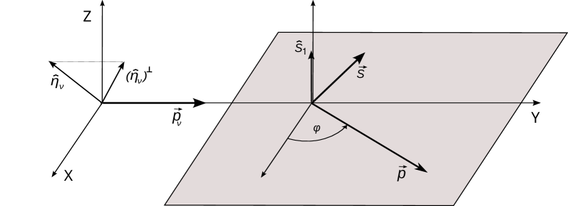
Figure 1: The neutrino scattering on the polarized electron: $\hat{\eta}_{\nu}$ is the unit polarization vector of incoming neutrino in its rest frame. $\hat{\eta}_{\nu}^{\perp}\equiv(\hat{\eta}_{\nu})^{\perp}$ is the transversal component of $\hat{\eta}_{\nu}$; $\hat{s}_{1}$ is the unit electron polarization vector of the target, $\vec{s}$ is the recoil electron polarization vector, $\vec{p}$ is the recoil electron momentum, $\varphi$ is the azimuthal angle of the outgoing electron momentum.

3 Time reversal violation — case of longitudinal neutrino polarization

In this section we consider $\rm VA,S_{L},T_{L}$ interactions and analyze the effects of TRSV assuming that the incoming beam of longitudinally polarized neutrinos scatters on the polarized electron target and the recoil electron momentum and its polarization are measured. As a result, mixed triple products can appear multiplied by the imaginary part of the products between the exotic scalar and tensor couplings or between the tensor and pseudoscalar couplings. We discuss various experimental settings allowing unambiguous detection of the signals generated by triple angular correlations. To this end we assume that the electron target is polarized perpendicularly to the direction of the incoming neutrino beam ($\hat{p}_{\nu}\cdot\hat{s}_{1}=0$). To extract terms breaking the time reversal symmetry we further assume that the scattered electrons are recorded only in the plane perpendicular to the polarization of the electron target ($\hat{p}\cdot\hat{s}_{1}=0$), and events are collected for the two opposite directions of the target polarization. The difference of cross sections taken for $\pm\hat{s}_{1}$ denoted by $\Omega$, eliminates many terms that do not depend on $\hat{s}_{1}$ vector; the relevant formulas can be found in the appendix A, Eqs. (10)-(13). The cross section $\Omega$ consisting of the quadratic terms $|\rm M_{VA}|^{2}$, $|\rm M_{S_{L}}|^{2}$, $|\rm M_{T_{L}}|^{2}$ and the interference term $2\Re(\rm M_{S_{L}}M^{*}_{T_{L}})$, has the structure ${\rm A}\,\hat{s}_{1}\cdot\vec{s}+{\rm B}\,\hat{p}_{\nu}\cdot(\hat{s}_{1}\times\vec{s})+{\rm C}\,\hat{p}\cdot(\hat{s}_{1}\times\vec{s})$. There are three possible ways to eliminate contributions from all time reversal invariant terms.

In the first method one assumes the condition $\hat{s}_{1}\cdot\vec{s}=0$ which amounts to the detection of the outgoing electron polarization in the scattering plane. This removes all supposedly dominating quadratic terms, and leaves us solely with the two triple products ${\rm B}\,\hat{p}_{\nu}\cdot(\hat{s}_{1}\times\vec{s})+{\rm C}\,\hat{p}\cdot(\hat{s}_{1}\times\vec{s})$. With an additional restriction that the experiment registers only the orthogonal polarization component of the scattered electron (i.e. $\vec{s}=\pm\hat{s}_{1}\times\hat{p}$), one obtains for the interference

$$2\Re(\rm M_{S_{L}}M^{*}_{T_{L}}) = \pm 16|c_{\rm S_{R}}||c_{\rm T_{R}}|mE_{\nu}^{3/2}\sqrt{y}\sin{(\theta_{\rm T,R}-\theta_{\rm S,R})}(2m+E_{\nu}y)$$ (2)

$$\left(\sqrt{2m+E_{\nu}y}-\sqrt{E_{\nu}y}\sin{\varphi}\right)$$

(the relevant symbols are defined in the appendix A).

The second method employs the observable $\Omega(\hat{p})-\Omega(-\hat{p})$ in the experiment counting events coming from two opposite momentum directions of the recoil electrons. As in the previous case the quadratic contributions are annihilated, and only $\hat{p}$-dependent mixed product $\hat{p}\cdot(\hat{s}_{1}\times\vec{s})$ survives.

The third approach relies on the restriction of the polarization measurement to its parallel component. In this case $\hat{s}_{1}\cdot\vec{s}=0$ and $\hat{p}\cdot(\hat{s}_{1}\times\vec{s})=0$, thus one is left only with the $\hat{p}_{\nu}$-dependent triple product $\hat{p}_{\nu}\cdot(\hat{s}_{1}\times\vec{s})$.

We conclude with the remark valid for each of the above method that any nonzero signal indicates the presence of the nonstandard time reversal violating $\rm S_{L}$, $\rm T_{L}$ interactions. It can be also seen that the contributions responsible for the time reversal violation survive, even if the cross section is integrated over the recoil electron energy. In consequence, this may improve the detectability of the expected effect.

4 Time reversal violation — scenario with transversal neutrino polarization

In this section we consider the possibility of time reversal violation in the presence of $\rm VA,S_{L},S_{R}$ interactions when the incoming neutrino beam has the nonzero transversal polarization components and scatters on the polarized electron target. It is assumed that both the recoil electron momentum and its polarization are measured. In this case, mixed products containing the transverse neutrino polarization vector appear, which are linear in exotic couplings. To isolate the time reversal violation contributions we impose the following conditions defining the experimental setup, $\hat{p}\cdot\hat{s}_{1}=0$, $\hat{p}\cdot\hat{s}=0$, $\hat{s}_{1}\cdot\hat{s}=0$ (i.e. the three vectors, target polarization vector, outgoing electron polarization and outgoing electron momentum, form an orthonormal basis).

In the first step in analogy with [12, 13, 14] we consider probabilities of emission of electrons having spins in two opposite directions (definition of the relevant cross section denoted by $\Delta$ is given in the appendix B). This observable eliminates exotic squared amplitude $|M_{\rm S_{R}}|^{2}$ and the interference between $S_{L}$ and $S_{R}$ couplings leaving the standard $|M_{\rm VA}|^{2}$ proportional to $\hat{p}_{\nu}\cdot\vec{s}$. The resulting interference term in the cross section includes linear combination of all possible triple scalar products, $\hat{s}_{1}\cdot(\hat{\eta}_{\nu}^{\perp}\times\vec{s})$, $\hat{p}_{\nu}\cdot(\hat{\eta}_{\nu}^{\perp}\times\vec{s})$, $\hat{p}\cdot(\hat{\eta}_{\nu}^{\perp}\times\vec{s})$, $\hat{p}_{\nu}\cdot(\hat{s}_{1}\times\vec{s})$, $\hat{p}\cdot(\hat{s}_{1}\times\vec{s})$; explicit formulas can be found in the appendix B. For unambiguous detection of the exotic $\rm VA-S_{R}$ interference one should be able to eliminate a dominating strong contribution from the standard squared amplitude $|M_{\rm VA}|^{2}$.

In the second step one attempts to get rid of $|M_{\rm VA}|^{2}$ contribution and separate different time reversal breaking contributions coming from specific triple products. Eq. (B) shows that a possible way is to assume $\hat{p}_{\nu}\cdot\vec{s}=0$, but this restriction is too severe (it holds when the scattered electrons are parallel to the incoming neutrinos) and renders this method very inefficient. In the second approach one further specialize the experimental setting taking a difference of cross sections for two opposite directions of target polarization $\pm\hat{s}_{1}$ (definition of the relevant cross section denoted by $\tilde{\Delta}$ is given in the appendix B). As a result $|M_{\rm VA}|^{2}$ vanishes and one is left solely with a linear combination of $\hat{s}_{1}$-dependent triple products, $\hat{s}_{1}\cdot(\hat{\eta}_{\nu}^{\perp}\times\vec{s})$, $\hat{p}_{\nu}\cdot(\hat{s}_{1}\times\vec{s})$, $\hat{p}\cdot(\hat{s}_{1}\times\vec{s})$ (see Eq. (B)). One then concludes that any nonzero result of the experiment confirms the presence of the exotic time reversal violating $\rm S_{R}$ interaction.

With the hypothetical assumption of the source producing neutrinos with a fixed (but unknown) orientation of the transversal polarization one can determine the value of the product $|\hat{\eta}_{\nu}^{\perp}|\Im{(c_{S_{R}})}$. This can be achieved only when the orientation of $\hat{\eta}_{\nu}^{\perp}$ polarization vector is known. To identify the direction of $\hat{\eta}_{\nu}^{\perp}$ one repeats the experiment with $\hat{s}_{1}$ rotated in the plane orthogonal to $\hat{p}_{\nu}$ keeping conditions $\hat{p}\cdot\hat{s}_{1}=0$, $\hat{p}\cdot\hat{s}=0$, $\hat{s}_{1}\cdot\hat{s}=0$, unchanged. It is now straightforward to recognize a direction $\hat{s}_{1}$ parallel to $\hat{\eta}_{\nu}^{\perp}$: indeed, in this case both $\hat{s}_{1}\cdot(\hat{\eta}_{\nu}^{\perp}\times\vec{s})$ and $\hat{p}\cdot\hat{\eta}_{\nu}^{\perp}$ vanish, so the net result is zero. Denoting now by $\varphi_{\nu}$ an angle between $\hat{s}_{1}$ and $\hat{\eta}_{\nu}^{\perp}$ (oriented from $\rm Z$ to $\rm X$ axis, Fig. 1) one obtains the following formula for the interference:

$$2\Re(\rm M_{VA}M^{*}_{S_{R}}) = -8|\hat{\eta}_{\nu}^{\perp}|\Im{(c_{S_{R}})}m\sqrt{y}\cos{\varphi}\sin{\varphi_{\nu}}\Bigl{(}\sin{\varphi}\bigl{(}E_{\nu}\left(2m+E_{\nu}y)\right)^{3/2}$$ (3)

$$-E_{\nu}\sqrt{y}\left(m+E_{\nu}\right)\left(2m+E_{\nu}y\right)\Bigr{)}.$$

In summary, knowing the orientation of the neutrino polarization vector the only quantity to fit the data is $|\hat{\eta}_{\nu}^{\perp}|\Im{(c_{S_{R}})}$. Similarly, as in the scenario considered in Sec. 3, the cross section can be integrated over the outgoing electron energy, potentially increasing the number of events.

5 Conclusions

The paper investigated several scenarios for the time reversal violation in the elastic scattering of Dirac neutrinos on polarized electrons, with the incoming neutrino beam being either longitudinally or transversely polarized, under the assumption that the momentum and polarization of the scattered electrons are observed.

In the case of longitudinal neutrino polarization, it is possible to unambiguously isolate two angular correlations that break the symmetry of time reversal. First, $\hat{p}_{\nu}\cdot(\hat{s}_{1}\times\vec{s})$, is composed of the incoming neutrino momentum, target polarization and polarization of the scattered electron. Second, $\hat{p}\cdot(\hat{s}_{1}\times\vec{s})$, consists of recoil electron momentum, its polarization, and polarization of the target. The expected effect depends on the interference between the scalar and tensor interactions.

In the case of transverse neutrino polarization one can, again, clearly identify the contribution from the time reversal symmetry violation triple products. The transversal neutrino polarization enters three mixed products, $\hat{s}_{1}\cdot(\hat{\eta}_{\nu}^{\perp}\times\vec{s})$, $\hat{p}_{\nu}\cdot(\hat{\eta}_{\nu}^{\perp}\times\vec{s})$, $\hat{p}\cdot(\hat{\eta}_{\nu}^{\perp}\times\vec{s})$, and appears in various double products multiplying two previously mentioned time reversal symmetry breaking terms. All new effects are linear in the exotic scalar $S_{R}$ interaction of right chiral neutrinos (a similar regularity shows up for tensor $T_{R}$ or pseudoscalar $P_{R}$ interactions).

The high-precision tests considered in this work would be a major challenge for experimental groups, because strong sources of low-energy (monoenergetic) neutrinos, large polarized targets and detectors sensitive to the directionality of scattered electrons are demanded. Besides, measurements of the recoil electron polarization would also be a difficult task, although the detection methods by Mott scattering have been known for a long time and used in beta decay experiments. Potential measurement of effects associated with transverse neutrino polarization would require further research on the selection of a suitable neutrino source. In particular it is crucial to explain the role of exotic interactions in the production of neutrino beam with nonzero transverse polarization.

Appendix A Scenario with $\rm VA,S_{L,R},T_{L,R}$ interactions for longitudinally polarized neutrino

The laboratory differential cross section for $\hat{p}_{\nu}\cdot\hat{\eta}_{\nu}=-1$, $\hat{p}_{\nu}\cdot\hat{s}_{1}=0$ and $\hat{p}\cdot\hat{s}_{1}=0$ is defined as

$$\frac{d^{2}\sigma}{d\varphi d\,y}=\frac{G_{F}^{2}}{64\pi^{2}E_{\nu}\,m}\,|M_{\nu e}|^{2},\\$$ (4)

where

$$y:=\frac{T_{e}}{E_{\nu}}=\frac{m}{E_{\nu}}\frac{2\cos^{2}{\theta_{e}}}{(1+\frac{m}{E_{\nu}})^{2}-\cos^{2}{\theta_{e}}}$$

is the ratio of the kinetic energy of the recoil electron $T_{e}$ to the incoming $\nu_{e}$ energy $E_{\nu}$, and $m$ is the electron mass. The squared amplitudes have the form

$$|M_{\rm VA}|^{2} = \frac{-16m^{2}}{m+yE_{\nu}}\sqrt{\frac{E_{\nu}}{2m+yE_{\nu}}}\left\{-\left(\sqrt{y}\left(\sqrt{yE_{\nu}\left(2m+yE_{\nu}\right)}\left(\hat{s}_{1}\cdot\vec{s}+1\right)\right.\right.\right.$$ (5)

$$\left.\left.\left.+2(y-2)\,\,\hat{p}\cdot\vec{s}\,\,E_{\nu}\right)m^{2}+E_{\nu}\left((y-2)\,\hat{p}\cdot\vec{s}\,\,E_{\nu}y^{3/2}+\left(2\left(y^{2}-y+1\right)+\right.\right.\right.\right.$$

$$\left.\left.\left.\left.\left(y^{2}+2y-2\right)\hat{s}_{1}\cdot\vec{s}\right)\sqrt{E_{\nu}\left(2m+yE_{\nu}\right)}\right)m+y\left((y-2)y\right.\right.\right.$$

$$\left.\left.\left.+2(y-1)\hat{s}_{1}\cdot\vec{s}+2\right)\sqrt{E_{\nu}^{5}\left(2m+yE_{\nu}\right)}\right)c_{\rm A}^{2}+2c_{\rm V}c_{\rm A}E_{\nu}\left(2\sqrt{y}\,\hat{p}\cdot\vec{s}\,m^{2}+\right.\right.$$

$$\left.\left.\left((y-2)\left(y+\hat{p}_{\nu}\cdot\vec{s}\right)\sqrt{E_{\nu}\left(2m+yE_{\nu}\right)}-(y-4)\sqrt{y}\,\hat{p}\cdot\vec{s}\,\,E_{\nu}\right)m\right.\right.$$

$$\left.\left.+(y-2)y\left(\left(y+\hat{p}_{\nu}\cdot\vec{s}\right)\sqrt{E_{\nu}^{3}\left(2m+yE_{\nu}\right)}-\sqrt{y}\,\hat{p}\cdot\vec{s}\,\,E_{\nu}^{2}\right)\right)\right.$$

$$\left.+c_{\rm V}^{2}\biggl{(}y\left(\sqrt{E_{\nu}\left(2m+yE_{\nu}\right)}\left(\hat{s}_{1}\cdot\vec{s}+1\right)+2\sqrt{y}\,\hat{p}\cdot\vec{s}\,\,E_{\nu}\right)m^{2}\right.$$

$$\left.\left.+E_{\nu}\left((y+4)\,\hat{p}\cdot\vec{s}\,\,E_{\nu}y^{3/2}+\left(-2\hat{p}_{\nu}\cdot\vec{s}y+2y+(y(y+2)-2)\hat{s}_{1}\cdot\vec{s}-2\right)\right.\right.\right.$$

$$\left.\left.\left.\sqrt{E_{\nu}\left(2m+yE_{\nu}\right)}\right)m-y\Bigl{(}\left(y\left(y+2\hat{p}_{\nu}\cdot\vec{s}-2\right)-2(y-1)\hat{s}_{1}\cdot\vec{s}+2\right)\right.\right.$$

$$\left.\sqrt{E_{\nu}^{5}\left(2m+yE_{\nu}\right)}-2y^{3/2}\,\hat{p}\cdot\vec{s}\,\,E_{\nu}^{3}\Bigr{)}\biggr{)}\right\}$$

$$|M_{\rm S_{\rm L}}|^{2} = 8m^{2}y\left|c_{S_{R}}\right|{}^{2}\left(\hat{s}_{1}\cdot\vec{s}+1\right)E_{\nu}\left(2m+yE_{\nu}\right)$$ (6)

$$|M_{\rm T_{\rm L}}|^{2} = \frac{-16m\left|c_{T_{R}}\right|{}^{2}}{m+yE_{\nu}}\sqrt{\frac{E_{\nu}}{2m+yE_{\nu}}}\biggl{(}-(y-2)y\left(\left(y+2\hat{p}_{\nu}\cdot\vec{s}-2\right)\sqrt{2m+yE_{\nu}}\right.$$ (7)

$$\left.\left.-2\,\hat{p}\cdot\vec{s}\,\sqrt{yE_{\nu}}\right)E_{\nu}^{5/2}+m\left((y-2)(y+4)\sqrt{yE_{\nu}}\,\hat{p}\cdot\vec{s}\,+\left(-2(y-2)\hat{p}_{\nu}\cdot\vec{s}\right.\right.\right.$$

$$\left.\left.\left.+y\left(y\hat{s}_{1}\cdot\vec{s}+4\right)-4\right)\sqrt{2m+yE_{\nu}}\right)E_{\nu}^{3/2}+m^{2}\sqrt{y}\left(\sqrt{yE_{\nu}\left(2m+yE_{\nu}\right)}\left(\hat{s}_{1}\cdot\vec{s}+1\right)\right.\right.$$

$$+2(y-2)\,\hat{p}\cdot\vec{s}\,E_{\nu}\Bigr{)}\biggr{)}$$

$$2\Re(\rm M_{S_{L}}M^{*}_{T_{L}}) = \frac{-16m\sqrt{y}E_{\nu}^{3/2}}{m+yE_{\nu}}\biggl{(}m\left(\Im\left(c_{S_{R}}\right)\Im\left(c_{T_{R}}\right)+\Re\left(c_{S_{R}}\right)\Re\left(c_{T_{R}}\right)\right)\Bigl{(}-\left(\hat{s}_{1}\cdot\vec{s}+1\right)$$ (8)

$$\left.E_{\nu}^{3/2}y^{5/2}+2\left(\hat{s}_{1}\cdot\vec{s}+1\right)\left(yE_{\nu}\right){}^{3/2}-m\left((y-2)\sqrt{2m+yE_{\nu}}\,\hat{p}\cdot\vec{s}\right.\right.$$

$$\left.\left.+\hat{s}_{1}\cdot\vec{s}\left(\sqrt{y^{3}E_{\nu}}-2\sqrt{yE_{\nu}}\right)+\sqrt{y^{3}E_{\nu}}\right)+2m\sqrt{yE_{\nu}}\right)-\left(\Im\left(c_{T_{R}}\right)\Re\left(c_{S_{R}}\right)\right.$$

$$\left.-\Im\left(c_{S_{R}}\right)\Re\left(c_{T_{R}}\right)\right)\left(m+yE_{\nu}\right)\left(\,\hat{p}\cdot\vec{s}\,\hat{p}_{\nu}\cdot(\hat{p}\times\hat{s}_{1})\sqrt{yE_{\nu}}\left(2m+yE_{\nu}\right)\right.$$

$$\left.+\hat{p}_{\nu}\cdot(\hat{s}_{1}\times\vec{s})\sqrt{yE_{\nu}}\left(2m+yE_{\nu}\right)+\left(2m\left(\hat{p}_{\nu}\cdot(\hat{p}\times\vec{s})+\hat{p}_{\nu}\cdot(\hat{p}\times\hat{s}_{1})\right)\right.\right.$$

$$\left.\left.-\hat{p}\cdot(\hat{s}_{1}\times\vec{s})\left(2m+yE_{\nu}\right)\right)\sqrt{2m+yE_{\nu}}\right)\biggr{)}$$

$$|M_{\rm T_{\rm R}}|^{2} = 0,\quad|M_{\rm S_{\rm R}}|^{2}=0$$

$$2\Re(\rm M_{S_{R}}M^{*}_{T_{R}}) = 0,\quad 2\Re(\rm M_{S_{L}}M^{*}_{S_{R}})=0$$

$$2\Re(\rm M_{S_{R}}M^{*}_{T_{L}}) = 0,\quad 2\Re(\rm M_{T_{L}}M^{*}_{T_{R}})=0$$

$$2\Re(\rm M_{S_{L}}M^{*}_{T_{R}}) = 0,\quad 2\Re(\rm M_{VA}M^{*}_{T_{L}})=0$$

$$2\Re(\rm M_{VA}M^{*}_{S_{L}}) = 0,\quad 2\Re(\rm M_{VA}M^{*}_{T_{R}})=0$$

$$2\Re(\rm M_{VA}M^{*}_{S_{R}}) = 0$$ (9)

If we take the difference of the cross sections $\Omega=\frac{1}{2}\left[\frac{d^{2}\sigma}{d\varphi d\,y}|_{\hat{s}_{1}}-\frac{d^{2}\sigma}{d\varphi d\,y}|_{(-\hat{s}_{1})}\right]$ for two opposite directions of target polarization ($\pm\hat{s}_{1}$) we obtain

$$|M_{\rm VA}|^{2} = 16m^{2}\hat{s}_{1}\cdot\vec{s}\left(c_{A}^{2}-c_{V}^{2}\right)E_{\nu}\left(my+2(y-1)E_{\nu}\right)$$ (10)

$$|M_{\rm S_{L}}|^{2} = 8m^{2}y\left|c_{S_{R}}\right|^{2}\hat{s}_{1}\cdot\vec{s}\,E_{\nu}\left(2m+yE_{\nu}\right)$$ (11)

$$|M_{\rm T_{L}}|^{2} = -16m^{3}y\left|c_{T_{R}}\right|^{2}\hat{s}_{1}\cdot\vec{s}\,E_{\nu}$$ (12)

$$2\Re(\rm M_{S_{L}}M^{*}_{T_{L}}) = \frac{-16m\sqrt{y}E_{\nu}^{3/2}}{m+yE_{\nu}}\Bigl{(}m\,\hat{s}_{1}\cdot\vec{s}\,\left(\Im\left(c_{S_{R}}\right)\Im\left(c_{T_{R}}\right)+\Re\left(c_{S_{R}}\right)\Re\left(c_{T_{R}}\right)\right)$$ (13)

$$\left(-E_{\nu}^{3/2}y^{5/2}+2\left(yE_{\nu}\right){}^{3/2}+2m\sqrt{yE_{\nu}}-m\sqrt{y^{3}E_{\nu}}\right)$$

$$-\left(\Im\left(c_{T_{R}}\right)\Re\left(c_{S_{R}}\right)-\Im\left(c_{S_{R}}\right)\Re\left(c_{T_{R}}\right)\right)\left(m+yE_{\nu}\right)\left(2m+yE_{\nu}\right)$$

$$\left(\hat{p}_{\nu}\cdot(\hat{s}_{1}\times\vec{s})\sqrt{yE_{\nu}}-\hat{p}\cdot(\hat{s}_{1}\times\vec{s})\sqrt{2m+yE_{\nu}}\right)\Bigr{)}$$

Appendix B Scenario with $\rm VA,S_{L},S_{R}$ interactions for $\hat{\eta}_{\nu}^{\perp}\neq 0$

The difference of cross sections $\Delta=\frac{1}{2}\left[\frac{d^{2}\sigma}{d\varphi d\,y}|_{\vec{s}}-\frac{d^{2}\sigma}{d\varphi d\,y}|_{(-\vec{s})}\right]$ taken for two opposite spin directions of the recoil electron $\pm\hat{s}$ with $\hat{p}_{\nu}\cdot\hat{s}_{1}=0$ when orthonormality conditions are requested, i.e. $\hat{p}\cdot\hat{s}_{1}=0,\hat{p}\cdot\hat{s}=0,\hat{s}\cdot\hat{s}_{1}=0$ has the form

$$|M_{\rm VA}|^{2} = -16c_{\rm V}m^{2}E_{\nu}^{2}\left(\hat{p}_{\nu}\cdot\hat{\eta}_{\nu}-1\right)\hat{p}_{\nu}\cdot\vec{s}\left(c_{\rm V}y-c_{\rm A}\left(y-2\right)\right)$$

$$|M_{\rm S_{R}}|^{2} = 0,\quad|M_{\rm S_{L}}|^{2}=0,\quad 2\Re(\rm M_{\rm S_{L}}M^{*}_{\rm S_{R}})=0,\quad 2\Re(\rm M_{\rm VA}M^{*}_{\rm S_{L}})=0$$

$$2\Re(\rm M_{\rm VA}M^{*}_{\rm S_{R}}) = A_{0}\,+A_{1}\,\hat{s}_{1}\cdot(\hat{\eta}_{\nu}^{\perp}\times\vec{s})+A_{2}\,\hat{p}_{\nu}\cdot(\hat{\eta}_{\nu}^{\perp}\times\vec{s})+A_{2}\,\hat{p}\cdot(\hat{\eta}_{\nu}^{\perp}\times\vec{s})$$ (14)

$$+A_{4}\,\hat{p}_{\nu}\cdot(\hat{s}_{1}\times\vec{s})+A_{5}\,\hat{p}\cdot(\hat{s}_{1}\times\vec{s})$$

where the coefficients $A_{0},A_{1}$, $A_{2}$, $A_{3}$, $A_{4}$, $A_{5}$ are given by

$$A_{0} = -8mE_{\nu}\Re{(c_{\rm S_{R}})}\sqrt{y}\Bigl{(}\vec{s}\cdot\hat{\eta}_{\nu}^{\perp}\,m\sqrt{y}\left(E_{\nu}y\left(c_{\rm A}-c_{\rm V}\right)+2c_{\rm A}m+2c_{\rm V}E_{\nu}\right)$$

$$\quad-c_{\rm A}\,\hat{p}_{\nu}\cdot\vec{s}\,\hat{p}\cdot\hat{\eta}_{\nu}^{\perp}\,\sqrt{E_{\nu}\left(2m+E_{\nu}y\right)^{3}}+c_{\rm V}\,\hat{p}_{\nu}\cdot\vec{s}\,\hat{p}\cdot\hat{\eta}_{\nu}^{\perp}\,y\sqrt{E_{\nu}^{3}\left(2m+E_{\nu}y\right)}\Bigr{)}$$

$$A_{1} = 8c_{A}\Im{(c_{S_{R}})}m^{2}E_{\nu}y\left(2m+E_{\nu}y\right)$$

$$A_{2} = -8c_{A}\Im{(c_{S_{R}})}mE_{\nu}^{2}y\left(2m+E_{\nu}y\right)$$

$$A_{3} = 8\Im{(c_{S_{R}})}mE_{\nu}^{3/2}\sqrt{y\left(2m+E_{\nu}y\right)}\left(2c_{A}m+c_{A}E_{\nu}y+c_{V}my\right)$$

$$A_{4} = 8c_{A}\Im{(c_{S_{R}})}m\hat{p}\cdot\hat{\eta}_{\nu}^{\perp}\sqrt{y}\left(E_{\nu}\left(2m+E_{\nu}y\right)\right)^{3/2}$$

$$A_{5} = -8c_{A}\Im{(c_{S_{R}})}mE_{\nu}^{2}\hat{p}\cdot\hat{\eta}_{\nu}^{\perp}y\left(2m+E_{\nu}y\right)$$ (15)

If we additionally calculate the differences $\tilde{\Delta}=\frac{1}{2}\left[\Delta(\hat{s}_{1})-\Delta(-\hat{s}_{1})\right]$ of the obtained cross sections for two opposite directions of target polarization $\pm\hat{s}_{1}$, we get

$$|M_{\rm VA}|^{2} = 0$$

$$2\Re(\rm M_{VA}M^{*}_{S_{R}}) = B_{1}\,\hat{s}_{1}\cdot(\hat{\eta}_{\nu}^{\perp}\times\vec{s})+B_{2}\,\hat{p}_{\nu}\cdot(\hat{s}_{1}\times\vec{s})+B_{3}\,\hat{p}\cdot(\hat{s}_{1}\times\vec{s})$$ (16)

where the coefficients are given by $B_{1}=A_{1}$, $B_{2}=A_{4}$, $B_{3}=A_{5}$.

References

• [1] S. L. Glashow, Nucl. Phys. 22, 579 (1961)
• [2] S. Weinberg, Phys. Rev. Lett. 19, 1264 (1967)
• [3] A. Salam, A. Salam, in Elementary Particle Theory (Almquist and Wiksells, Stockholm, 1969)
• [4] R. P. Feynman, M. Gell-Mann, Phys. Rev. 109, 193 (1958)
• [5] E. C. G. Sudarshan, R. E. Marshak, Phys. Rev. 109, 1860 (1958)
• [6] J.H. Christenson, J.W. Cronin, V.L. Fitch and R. Turlay, Phys. Rev. Lett. 13, 138 (1964)
• [7] B. Aubert et al., Phys. Rev. Lett. 87, 091801 (2001)
• [8] K. Abe et al., Phys. Rev. Lett. 87, 091802 (2001)
• [9] M. Kobayashi, T. Maskawa, Prog. Theor. Phys. 49, 652 (1973)
• [10] A. Riotto, M. Trodden, Annu. Rev. Nucl. Part. Sci. 49, 35 (1999)
• [11] K. Bodek et al., EPJ Web of Conferences 262, 01014 (2022)
• [12] J. Jackson et al., Phys. Rev. 106, 517 (1957)
• [13] J. Jackson et al., Nucl. Phys. 4, 206 (1957)
• [14] M. E. Ebel et al., Nucl. Phys. 4, 213 (1957)
• [15] S. Weinberg, Phys. Rev. D 42, 860 (1990)
• [16] R. Garisto, G. L. Kane, Phys. Rev. D 44, 2038 (1991)
• [17] G. Belanger, C. Q. Geng, Phys. Rev. D 44, 2789 (1991)
• [18] G. H. Wu, J. N. Ng. Phys.Lett. B 392, 93 (1997)
• [19] E. Gabrielli, Phys. Lett. B 301, 409 (1993)
• [20] S. Geer, Phys. Rev. D 57, 6989 (1998)
• [21] S. Geer, Phys. Rev. D 59, 039903 (1999)
• [22] W. Sobków, A. Błaut, Eur. Phys. J. C 78, 197 (2018)
• [23] J. Bernabeu et al., Phys. Lett. B 613, 162 (2005)
• [24] T. I. Rashba, V. B. Semikoz, Phys. Lett. B 479, 218 (2000)
• [25] P. Minkowski, M. Passera, Phys. Lett. B 541, 151 (2002)
• [26] S. Ciechanowicz et al., Phys. Rev. D 71, 093006 (2005)
• [27] A. Błaut, W. Sobków, Eur. Phys. J. C 80, 261 (2020)
• [28] J. Barranco et al., Phys. Lett. B 739, 343 (2014)
• [29] J. Barranco et al., J. Phys. G: Nucl. Part. Phys. 47, 035201 (2020)
• [30] V. A. Guseinov et al., Phys. Rev. D 75, 073021 (2007)
• [31] W.-T. Ni et al., Phys. Rev. Lett. 82, 2439 (1999)
• [32] W. Bialek et al., Phys. Rev. Lett. 56, 1623 (1986)
• [33] P. V. Vorobyov, Y. I. Gitarts, Phys. Lett. B 208, 146 (1988)
• [34] C.-T. Chiang, M. Kamionkowski, G. Z. Krnjaic, Phys. Dark Univ. 1, 109 (2012)
• [35] T. Franarin, M. Fairbairn, Phys. Rev. D 94, 053004 (2016)
• [36] G. D. Starkman, D. N. Spergel, Phys. Rev. Lett. 74, 2623 (1995)
• [37] R. Catena, K. Fridell, V Zema, JCAP 11, 018 (2018)
• [38] J.C. Pati, A. Salam, Phys. Rev. D 10, 275 (1974)
• [39] R. Mohapatra, J.C. Pati, Phys. Rev. D 11, 566 (1975)
• [40] R.N. Mohapatra, G. Senjanovic, Phys. Rev. D 12, 1502 (1975)
• [41] M. A. B. Beg et al., Phys. Rev. Lett. 38, 1252 (1977)
• [42] P. Herczeg, Phys. Rev. D 34, 3449 (1986)
• [43] A. Jodidio et al., Phys. Rev. D 34, 1967 (1986)
• [44] E. J. Eichten, K. D. Lane, M.E. Peskin, Phys. Rev. Lett. 50, 811 (1983)
• [45] P. Herczeg, Prog. Part. Nucl. Phys. 46, 413 (2001)
• [46] N. Arkani-Hamed, S. Dimopoulous, G. Dvali, J. March-Russell, Phys. Lett. B 429, 263 (1998).
• [47] T. Banks, A. Zaks, Nucl. Phys. B 196, 189 (1982)
• [48] H. Georgi, Phys. Rev. Lett. 98, 221601 (2007)
• [49] H. Georgi, Phys. Lett. B 650, 275 (2007)
• [50] M. Misiaszek et al., Nucl. Phys. B 734, 203 (2006)
• [51] B. Babussinov et al., Nucl. Instrum. and Meth. A 694, 335 (2012)
• [52] M. A. Bouchiat, T. R. Carver, C. M. Varnum, Phys. Rev. Lett. 5, 373 (1960)
• [53] T. G. Walker, W. Happer, Rev. Mod. Phys. 69, 629 (1997)
• [54] S. Ciechanowicz, M. Misiaszek, S. Sobków, Eur. Phys. J. C 32, s01, s151 (2003)
• [55] R. L. Workman et al. (Particle Data Group), Prog. Theor. Exp. Phys. 2022, 083C01 (2022)
• [56] L. Michel, A. S. Wightman, Phys. Rev. 98, 1190 (1955)