Dynamics of Entanglement Generation and Transfer

Abstract

We show that the generating and transfer of entanglement during adiabatic interactions can be traced to a succession of avoided energy level crossings at which eigenvalues swap their eigenvectors. These swaps of eigenvectors weave the entanglement in multi-partite systems. The efficiency of this weaving of entanglement depends on the narrowness of the avoided level crossings and it is, therefore, constraining the speed of adiabatic evolution. This relates an adiabatic quantum computation’s complexity, as measured by its minimum duration, to that quantum computation’s usage of the resource of entanglement. To derive these results, we employ the spectral theorem to decompose interaction Hamiltonians into rank-one projectors and we then use the adiabatic theorem to successively adiabatically introduce these projectors. For each projector activation, using recent exact results on the behaviour of eigensystems under the addition of Hamiltonians, we can then non-perturbatively calculate the entanglement dynamics. Our findings provide new tools for the analysis and control of the dynamics of entanglement.

I Introduction

Entanglement, as a phenomenon without classical analog, is of fundamental theoretical importance as well as an essential resource in quantum technologies. Here, we analyze the generating and transmission of entanglement during adiabatic interactions. This includes the interactions in adiabatic quantum computing [1, 2, 3, 4, 5, 6], which is known to be equivalent to algorithmic quantum computing up to polynomial overhead [7].

I.1 Setup

In order to analyze the basic processes underlying the generating and transmission of entanglement, we here consider a setup consisting of three systems, $\tilde{A}$, $A$ and $B$. We take their Hilbert space to be finite-dimensional, which is justified as long as the systems possess a finite size and a finite energy budget. Systems $\tilde{A}$ and $A$ are assumed to be initially entangled. During the subsequent unitary time evolution, systems $A$ and $B$ interact adiabatically while system $\tilde{A}$ remains a non-interacting ancilla, as illustrated in Figure 1. This setup allow us to analyze not only how the interaction generates entanglement between $A$ and $B$, but also how it can transfer $\tilde{A}$’s initial entanglement with $A$ to system $B$ or system $AB$.

Within this setup, we will relate the efficiency of the transfer of entanglement to the narrowness of avoided level crossings and, therefore, to the speed of adiabatic evolution. This offers new tools for relating a quantum computation’s need for the resource of quantum entanglement to that quantum computation’s complexity as measured by its minimum duration. As technical tools, we introduce Renyi entropy-based measures of coherent information for both the direct quantum channel from $A$ to $A^{\prime}$ and for the complementary channel from $A$ to $B^{\prime}$.

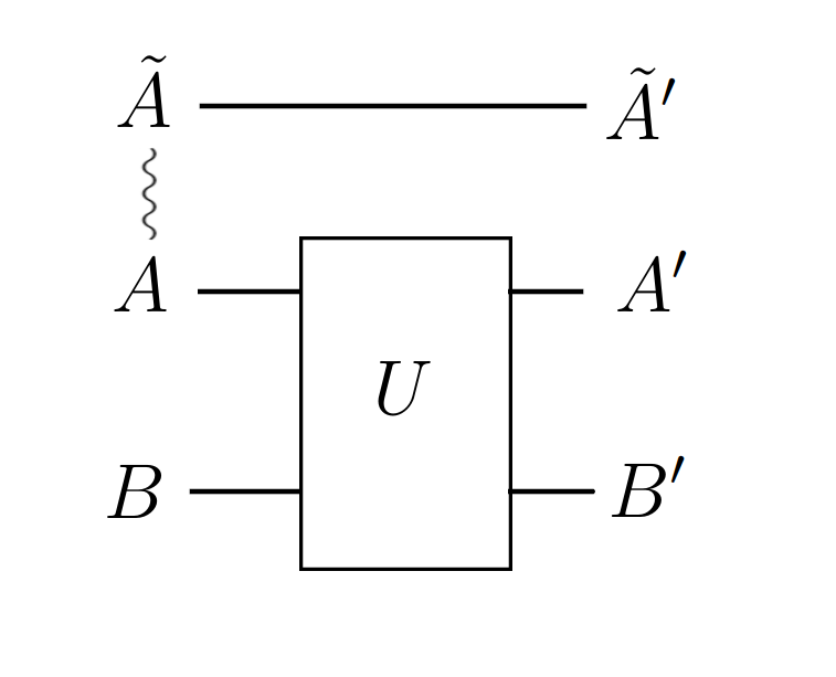
Figure 1: Systems $\tilde{A}$ and $A$ are prepared in an entangled state. The time evolution operator, $U$, is adiabatically generated by a Hamiltonian which acts non-trivially only on system $AB$.

I.2 Methods

We consider the dynamics generated by a generic Hamiltonian of the form $H_{0}+g(t)H_{int}$ where $g(t)$ increases from zero to $g(T)$ slowly enough for the evolution to be adiabatic. We decompose this evolution into manageable segments by employing the spectral and adiabatic theorems. First, we use the spectral theorem to decompose $H_{int}$ into rank-one projectors, $H_{int}=\sum_{n}\lambda_{n}\outerproduct{v_{n}}{v_{n}}$. We then employ the adiabatic theorem to reschedule the adiabatic evolution by sequentially adiabatically adding, or ‘activating’, these projectors: in order to arrive at the final Hamiltonian $H_{0}+g(T)H_{int}$, we start with $H_{0}$ and then one by one we adiabatically add $\mu_{n}|v_{n}\rangle\langle v_{n}|$ by swiping the prefactor $\mu_{n}$ of each projector $\outerproduct{v_{n}}{v_{n}}$ from $\mu_{n}=0$ to $\mu_{n}=g(T)\lambda_{n}$.

Each of these adiabatic activations of a rank-one projector takes the form

$$H(\mu)=D+\mu\outerproduct{v}{v}$$ (1)

where $D$ is the Hamiltonian before the new activation, $\outerproduct{v}{v}:=\outerproduct{v_{n}}{v_{n}}$ is the projector that is next to be activated, and $\mu$ is adiabatically swept from the initial $\mu=0$ to its final value $\mu=g(T)\lambda_{n}$.

Our overall task, which is to track the evolution of the entanglement in the system $\tilde{A}AB$, is thereby decomposed into a sequence of more manageable tasks: for each activation of a projector, track the evolution of the eigenvalues $s_{n}(\mu)$ and eigenvectors $|s_{n}(\mu)\rangle$ in $H(\mu)|s_{n}(\mu)\rangle=s_{n}(\mu)|s_{n}(\mu)\rangle$ as $\mu$ runs from $\mu=0$ to its final value $\mu=g(T)\lambda_{n}$. This is a useful decomposition because it allows us to recruit the recent results in [8], which nonperturbatively describe the evolution of the eigenvalues $s_{n}(\mu)$ and eigenstates $|s_{n}(\mu)\rangle$ of self-adjoint operators $H(\mu)$ for all $D$ and $|v\rangle$, in finite-dimensional Hilbert spaces.

By applying these methods to the interactions in the multi-partite system $\tilde{A},A,B$, we will show that, during each activation of a new projector, the generating and transfer of entanglement decomposes into a succession of avoided level crossings at which, crucially, the two involved eigenvalues swap their eigenvectors. These swappings of eigenvectors are, in this sense, weaving the entanglement.

I.3 Structure of the paper

• Section II provides an intuitive overview of key findings, highlighting conceptual points and using visualization.

• Section III introduces several lemmas that serve as basic mathematical preliminaries.

• Section IV establishes conditions for maximizing the transfer or preservation of entanglement during the adiabatic interactions of $A$ and $B$.

• Sections V and VI demonstrate that complete entanglement transfer, or preservation, induces a clearly structured evolution of the eigenspectrum and eigenvectors of the total time-dependent Hamiltonian of the system $\tilde{A}AB$. Further, a link is established between the entanglement dynamics and the permutation group.

• Section VII demonstrates a direct relationship between the maximum speed of an adiabatic quantum computation on one hand, and that computation’s generating and transfer of the resource of entanglement. This is achieved by relating the narrowness of the gaps in avoided level crossings to the efficiency of entanglement generation and transfer in those avoided level crossings.

• Section VIII introduces and applies measures of coherent information that are useful for non-perturbative quantifying the transfer of entanglement among subsystems.

II Intuitive overview of the results

As indicated above, we are decomposing any given generic adiabatic dynamics into a succession of adiabatic additions, or ‘activations’, of rank one projectors. During each new activation of a projector, our task is, therefore, to track the evolution of the eigenvectors and eigenvalues of a Hamiltonian of the form $H(\mu)=D+\mu\outerproduct{v}{v}$, where $\mu$ is adiabatically swept from $\mu=0$ to its final value $\mu=g(T)\lambda_{n}$. Here, $D$ is the Hamiltonian at the end of the prior activation. With the notation $D|d_{n}\rangle=d_{n}|d_{n}\rangle$, we have $d_{n}=s_{n}(0)$ and $|d_{n}\rangle=|s_{n}(0)\rangle$.

During each of these activations, i.e., as a $\mu$ is adiabatically swept from $\mu=0$ to its final value $\mu=g(T)\lambda_{n}$, a succession of avoided level crossings occurs [8]. As we will show in the present paper, if the system is subdivided into subsystems, it is at these avoided level crossings that the generation and transfer of entanglement among the subsystems occurs. This is because at each avoided level crossing, a pair of eigenvalues swaps their eigenvectors.

This key dynamics is most clearly seen in those cases where $|v\rangle$ is not parallel but almost parallel to an initial eigenvector $|s_{n}(0)\rangle=\ket{d_{n}}$ of the initial Hamiltonian $D$. In these cases, which we will call edge cases, any changes of the entanglement among $\tilde{A}$, $A$, and $B$ while adiabatically sweeping $\mu$ from $\mu=0$ to $\mu=g(T)\lambda_{n}$ always occur suddenly at specific values of $\mu$ that we will call critical $\mu$ values. It is at these critical $\mu$ values that the crossing of two energy eigenvalues, say $s_{n}(\mu)$ and $s_{n+1}(\mu)$ is narrowly avoided while these two eigenvalues quickly swap their eigenvectors, $|s_{n}(\mu)\rangle$ and $|s_{n+1}(\mu)\rangle$, thereby in this sense weaving entanglement among the subsystems. In the non-edge cases, characterized by generic $\ket{v}$, the behaviour remains qualitatively the same, except that the level crossings are avoided with greater gaps, and the eigenvector swaps are less sudden.

The fact that in edge cases, i.e., for narrow gaps, each involved eigenvector evolves into an orthogonal and therefore very different eigenvector over a very small range of values of $\mu$ implies that these $\mu$-values need to be traversed particularly slowly for the evolution to remain adiabatic. As we will discuss below, this relates an adiabatic quantum computation’s use of the resource of entanglement to the maximum speed of that computation.

In the body of the paper we will present further findings, such as a relation between the rate of entanglement transfer and the narrowness of an avoided level crossings, which subsequently determines the minimum duration of the adiabatic evolution. We will also non-perturbatively quantify the flow of quantum information through both the direct and complementary channels, i.e., from $A$ to $A^{\prime}$ and from $A$ to $B^{\prime}$.

First, however, it will be useful to postpone the mathematical details and instead establish intuition and visualizations for the dynamics of the weaving of entanglement that we discussed above. To this end, let us first visualize the dynamics of eigenvalues and eigenvectors under adiabatic activation for a total system. Second, we apply this to visualize the generation of entanglement among subsystems $A$ and $B$. Third, we visualize the transfer of entanglement among subsystems by visualizing how system $\tilde{A}$, which was initially entangled with $A$ can become entangled with $B$ or $AB$ instead.

II.1 Visualization of the dynamics of eigenvectors and eigenvalues during an adiabatic activation

As outlined above, we decompose the general problem into segments of adiabatic evolution, each of which is described by a Hamiltonian of the form of (1).

We begin by visualizing the dynamics of the eigenvalues. In the simplest case, $|v\rangle$ equals one of the eigenvectors of $D$, i.e., $|v\rangle=|d_{i}\rangle=|s_{i}(0)\rangle$. The adiabatic evolution is trivial in this case, as all eigenvectors stay the same and also all eigenvalues are constant, $s_{n}(\mu)=s_{n}(0)=d_{n}$, except for $n=i$ where we have $s_{i}(\mu)=s_{i}(0)+\mu$. Since $s_{i}(\mu)$ is the only eigenvalue that changes, it crosses the levels of all other eigenvalues, see the blue line in Figure 2.a.

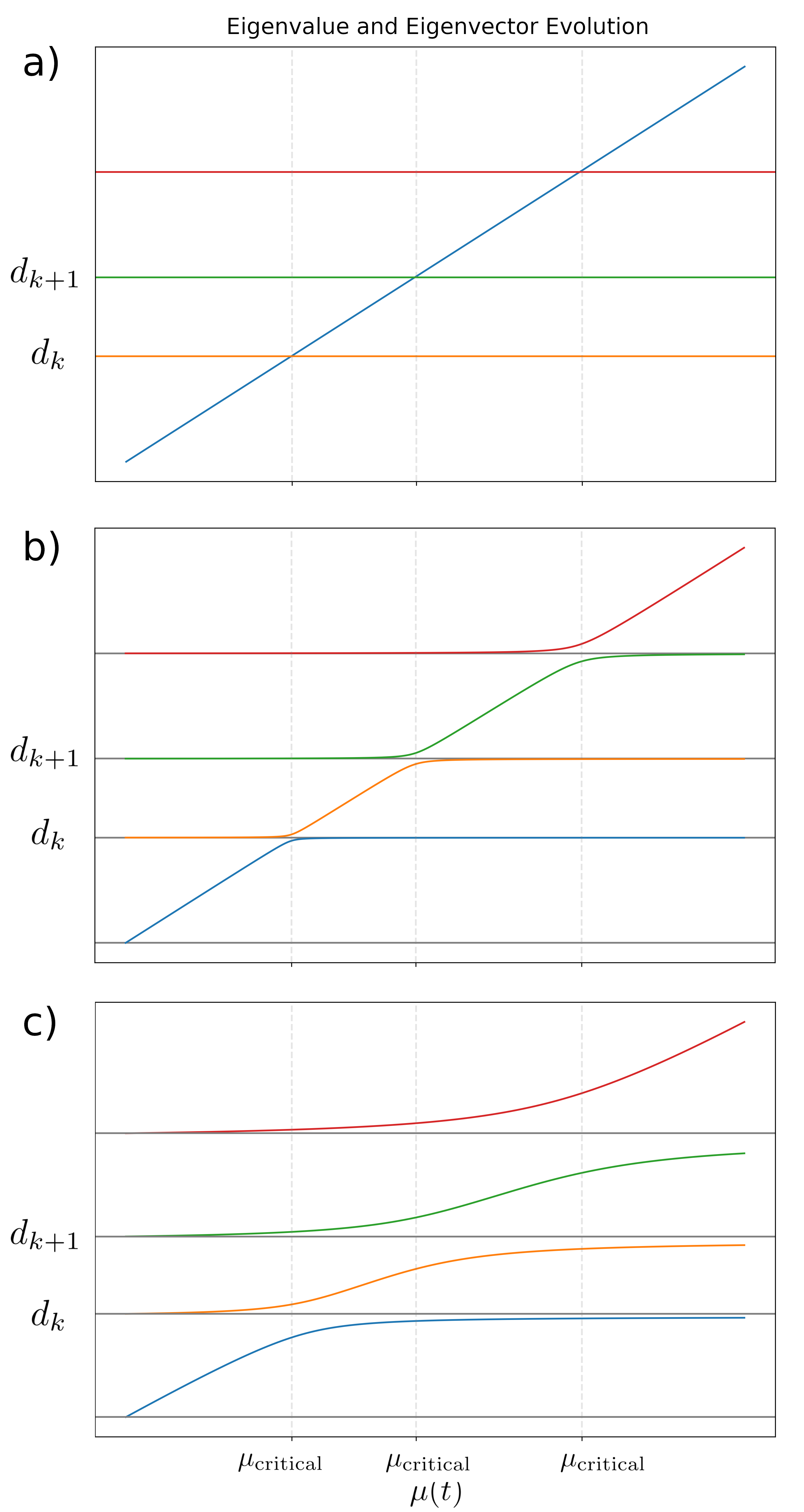
Figure 2: The dynamics of the eigenvalues of $H(\mu)$ for a generic choice of $D$ and with $|v\rangle$ chosen to be a) a trivial case, b) an edge case and c) a non-edge case.

Now let us consider what we call an edge case, i.e., a case where $|v\rangle$ is not equal to but close to one of the eigenvectors of $D$, i.e.: $|v\rangle\approx|d_{i}\rangle=|s_{i}(0)\rangle$ for a fixed $i$. The adiabatic behaviour is now very different: as illustrated in Figure 2.b, all level crossings are narrowly avoided as $\mu$ runs through the reals. We call the values of $\mu$ at which these level crossing avoidances occur the critical $\mu$ values. The eigenvalue that is increasing while $\mu$ runs through $\mu=0$ is the eigenvalue $s_{i}(\mu)$.

The non-edge cases, i.e., when $|v\rangle$ is not close to an eigenvector of $D$, exhibit the same qualitative behaviour, see [8]: as $\mu$ runs from $\mu=-\infty$ to $\mu=+\infty$, all eigenvalues $s_{k}(\mu)$ strictly monotonically increase and all level crossings are avoided, though generally less narrowly. Each eigenvalue converges to the starting value of the next higher eigenvalue $s_{k+1}(\mu)$.

We now address the dynamics of the eigenvectors $|s_{k}(\mu)\rangle$. In the trivial cases, as in Figure 2.a, the eigenvectors do not change. In the edge cases, $|v\rangle\approx|d_{i}\rangle=|s_{i}(0)\rangle$ for a fixed $i$, as illustrated in Figure 2.b, let us consider the $k$’th eigenvalue, $d_{k}=s_{k}(0)$ of $D$. Initially, as $\mu$ is running from $\mu=0$ to larger values, $s_{k}(\mu)$ and its eigenvector remain approximately constant: $s_{k}(\mu)\approx s_{k}(0)=d_{k}$ and $|s_{k}(\mu)\rangle\approx|s_{k}(0)\rangle=|d_{k}\rangle$. Then, at a critical $\mu$ value, the eigenvalue $s_{k}(\mu)$ starts to grow, see Figure 2.b. At the same time, at this critical $\mu$ value, the eigenvector $|s_{k}(\mu)\rangle$ changes quickly from $|s_{k}(\mu)\rangle\approx|s_{k}(0)\rangle=|d_{k}\rangle$ to $|s_{k}(\mu)\rangle\approx|v\rangle$.

As $\mu$ grows further it eventually reaches the next critical $\mu$ value, where the eigenvalue $s_{k}(\mu)$ changes its eigenvector again, now from $|s_{k}(\mu)\rangle\approx|v\rangle$ to $|s_{k}(\mu)\rangle\approx|s_{k+1}(0)\rangle=|d_{k+1}\rangle$. This is illustrated in Figure 3. Notice that for $k=i$, we have $|s_{i}(\mu)\rangle\approx|v\rangle$ as $\mu$ passes through $\mu=0$.

Figure 3: The evolution of the eigenvalue $s_{k}(\mu)$ and eigenvector $|s_{k}(\mu)\rangle$ as a function of the parameter $\mu$. Annotations along the eigenvalue curve specify the eigenvector corresponding to $s_{k}(\mu)$. As $\mu$ runs from left to right, it passes two critical $\mu$ values, the eigenvector $|s_{k}(\mu)\rangle$ first transitions from $|s_{k}(\mu)\rangle\approx|s_{k}(0)\rangle=\ket{d_{k}}$ to $|s_{k}(\mu)\rangle\approx\ket{v}$ and then to $|s_{k}(\mu)\rangle\approx\ket{d_{k+1}}$.

The suddenness with which an eigenvalue changes its eigenvector as $\mu$ moves through a critical point is illustrated in Figure 4.

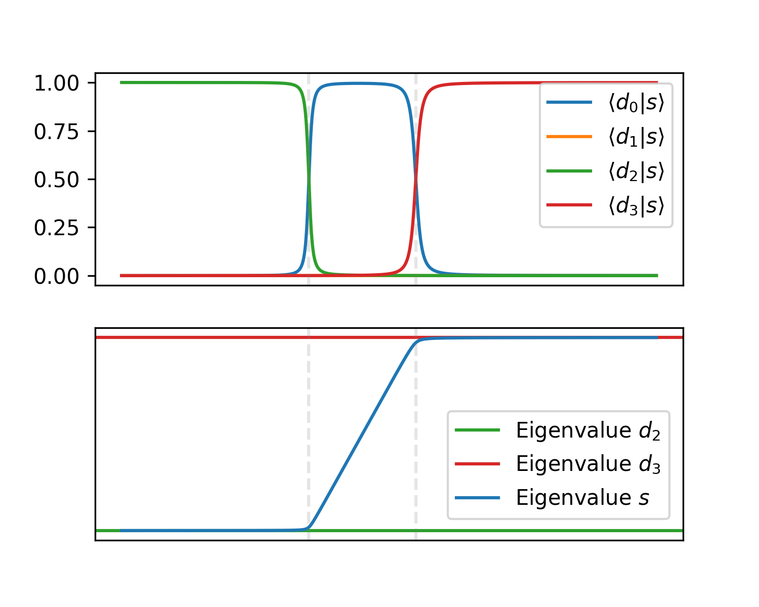
Figure 4: Example of an edge case with $\ket{v}\approx\ket{d_{0}}$, illustrating the eigenvalue $s_{k}(\mu)$ changing its eigenvector $|s_{k}(\mu)\rangle$ when passing through critical $\mu$ values (indicated by grey vertical dashed lines).

The larger picture is, as shown in Figure 2, that at each critical $\mu$ value two eigenvalues narrowly avoid crossing. Figure 5 visualizes what this means for the eigenvectors $|s_{k}(\mu)\rangle$ and $|s_{k+1}(\mu)\rangle$ of two eigenvalues $s_{k}(\mu)$ and $s_{k+1}(\mu)$ at a narrow crossing avoidance: the eigenvalues quickly trade their eigenvectors.

In later sections, we will show that the extent of crossing avoidance and suddenness of eigenvector change is determined by a single parameter $\epsilon$.

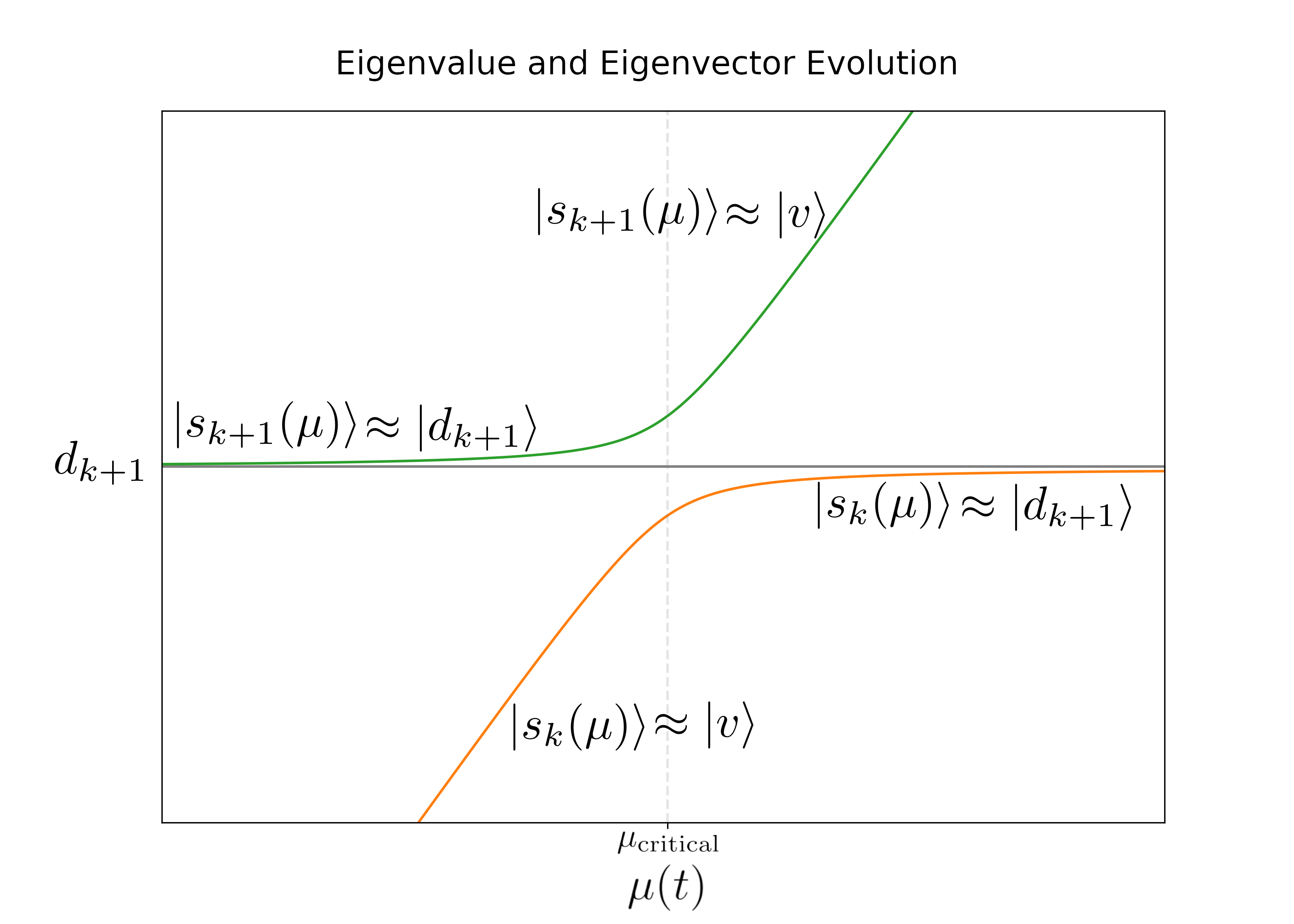
Figure 5: At a critical $\mu$ value, the eigenvalues $s_{k}(\mu)$ and $s_{k+1}(\mu)$ of $H(\mu)=D+\mu|v\rangle\langle v|$ trade their eigenvectors.

In non-edge cases, as in Figure 2.c, the situation is qualitatively the same. All level crossings are avoided, and the eigenvalues trade their eigenvectors, although the level crossings can be avoided less narrowly and can also occur at values other than the eigenvalues $d_{k}$. Further, during a phase in which an eigenvalue $s_{n}(\mu)$ quickly grows, its eigenvector $|s_{n}(\mu)\rangle$ need no longer approximate $|v\rangle$. See [8] for the details. In comparison, the edge cases are characterized by very narrow level crossing avoidances that occur suddenly, and the associated eigenvector swaps are correspondingly sudden. Hence, the edge cases offer sharper tools for analyzing or controlling entanglement dynamics. We will, therefore, pay particular attention to the edge cases.

II.2 Visualization of entanglement generation in the bi-partite system $AB$

By applying these findings to a system that is divided into two subsystems, $A$ and $B$, we can track the dynamics of the entanglement between $A$ and $B$ during adiabatic evolution. The analysis can be applied to any activation of a projector, i.e., with any starting Hamiltonian $D$. However, for the purpose of gaining intuition, it is convenient to consider an initial Hamiltonian $D$ that is of the typical form of a free Hamiltonian, $D=H_{A}\otimes I+I\otimes H_{B}$. We denote the spectra of $H_{A}$ and $H_{B}$ by $\{a_{i}\},\{b_{j}\}$ and we assume them to be generic, i.e., such that the spectrum of $D$ is non-degenerate. We denote the eigenbases of $A$ and $B$ by $\{|a_{i}\rangle\},\{|b_{j}\rangle\}$.

Further, when activating a projector $\outerproduct{v}{v}$, we will, for clarity, focus on edge cases, $|v\rangle\approx|a_{i}\rangle|b_{j}\rangle$, for fixed $i$ and $j$. The dynamics at each critical $\mu$ value can then be deduced from Figure 5: as two neighbouring energy eigenvalues narrowly avoid crossing at a critical $\mu$ value, they trade their eigenvectors: prior to reaching the critical $\mu$ value, the eigenvector $|s_{k}(\mu)\rangle$ of the eigenvalue $s_{k}(\mu)$ is $|s_{k}(\mu)\rangle\approx\ket{v}$, while the eigenvector $|s_{k+1}(\mu)\rangle$ associated with $s_{k+1}(\mu)$ is $|s_{k+1}(\mu)\rangle\approx\ket{d_{k+1}}$. Passing the critical $\mu$ value, the eigenvectors switch: the eigenvector $|s_{k}(\mu)\rangle$ belonging to the eigenvalue $s_{k}(\mu)$ transitions to $|s_{k}(\mu)\rangle\approx\ket{d_{k+1}}$, and the eigenvector $|s_{k+1}(\mu)\rangle$ belonging to the eigenvalue $s_{k+1}(\mu)$ transitions to $|s_{k+1}(\mu)\rangle\approx\ket{v}$. The application to the two-partite system $AB$ is illustrated in Figure 6,

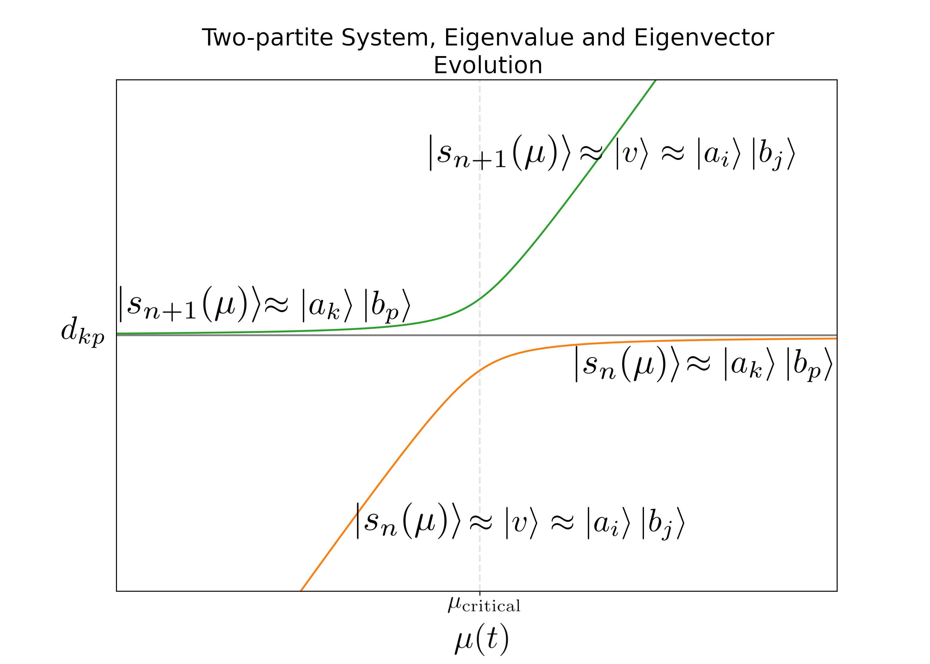
Figure 6: Eigenvector swap at a critical $\mu$ value, in a two-partite system $AB$.

where we can read off two observations on the dynamics of the entanglement in system $AB$:

Observation 1.

In edge cases, every initially unentangled state that is an energy eigenstate becomes briefly entangled during an avoided level crossing, but this entanglement does not persist after the avoided level crossing. To see this, we recall that every initial energy eigenstate is a product state $|a_{k}\rangle|b_{p}\rangle$. As $\mu$ is adiabatically swept, the eigenvalue of this product state moves, eventually avoiding a level crossing and swapping its eigenvector with the eigenvector of the neighbouring eigenvalue, which is also an initial energy eigenstate and, therefore, a product state. This means that in edge cases, energy eigenstates evolve into energy eigenstates and since neither is entangled, no entanglement is being generated. Except that during the brief period of the level crossing avoidance, i.e., close to a critical $\mu$, the continuity of the swapping of the eigenvectors implies that each of the two eigenvalues temporarily possesses an eigenvector that is a superposition of the two product states that are being swapped. This means that each of these evolving states is temporarily entangled during the level crossing avoidance. Of course, this otherwise temporary entanglement can be frozen by freezing the value of $\mu$ at the critical value.

Observation 2.

In edge cases, any initially unentangled state that is not an energy eigenstate can become entangled during an avoided level crossing, and this entanglement persists after the avoided level crossing. Assume, e.g., that system $AB$ was prepared in an unentangled state that is a superposition of energy eigenstates, such as the state $(|a_{k}\rangle+|a_{m}\rangle)|b_{p}\rangle$. During the time evolution, at a critical $\mu$ value, this state can become permanently entangled as, e.g., the state $|a_{k}\rangle|b_{p}\rangle$ can be swapped, for example, for the state $|a_{k}\rangle|b_{p+1}\rangle$, so that after the avoided level crossing our system is in the entangled state $|a_{k}\rangle|b_{p+1}\rangle+|a_{m}\rangle|b_{p}\rangle$. Unlike in the case of Observation 1 above, here the newly generated entanglement between $A$ and $B$ persists for values of $\mu$ larger than the critical $\mu$. In this sense, entanglement between $A$ and $B$ can be said to be ‘woven’ during an eigenvector swap at an avoided level crossing.

II.3 Visualization of entanglement transfer in the tri-partite system $\tilde{A}AB$

Similarly, in the tripartite system $\tilde{A}AB$, let us consider initial Hamiltonians of the form $D=H_{\tilde{A}}\otimes I\otimes I+I\otimes H_{A}\otimes I+I\otimes I\otimes H_{B}$ and activate a projector though $H(\mu)=D+\mu(I\otimes\outerproduct{v}{v})$ which acts on the Hilbert space $\mathcal{H}_{A}\otimes\mathcal{H}_{B}$. Similar to the two-partite case, the structure of the entanglement in the tri-partite system $\tilde{A}AB$ can only change when eigenvalues avoid crossing and thereby swap their eigenvectors. Again, this is particularly clear in edge cases, as is illustrated in Fig.7,

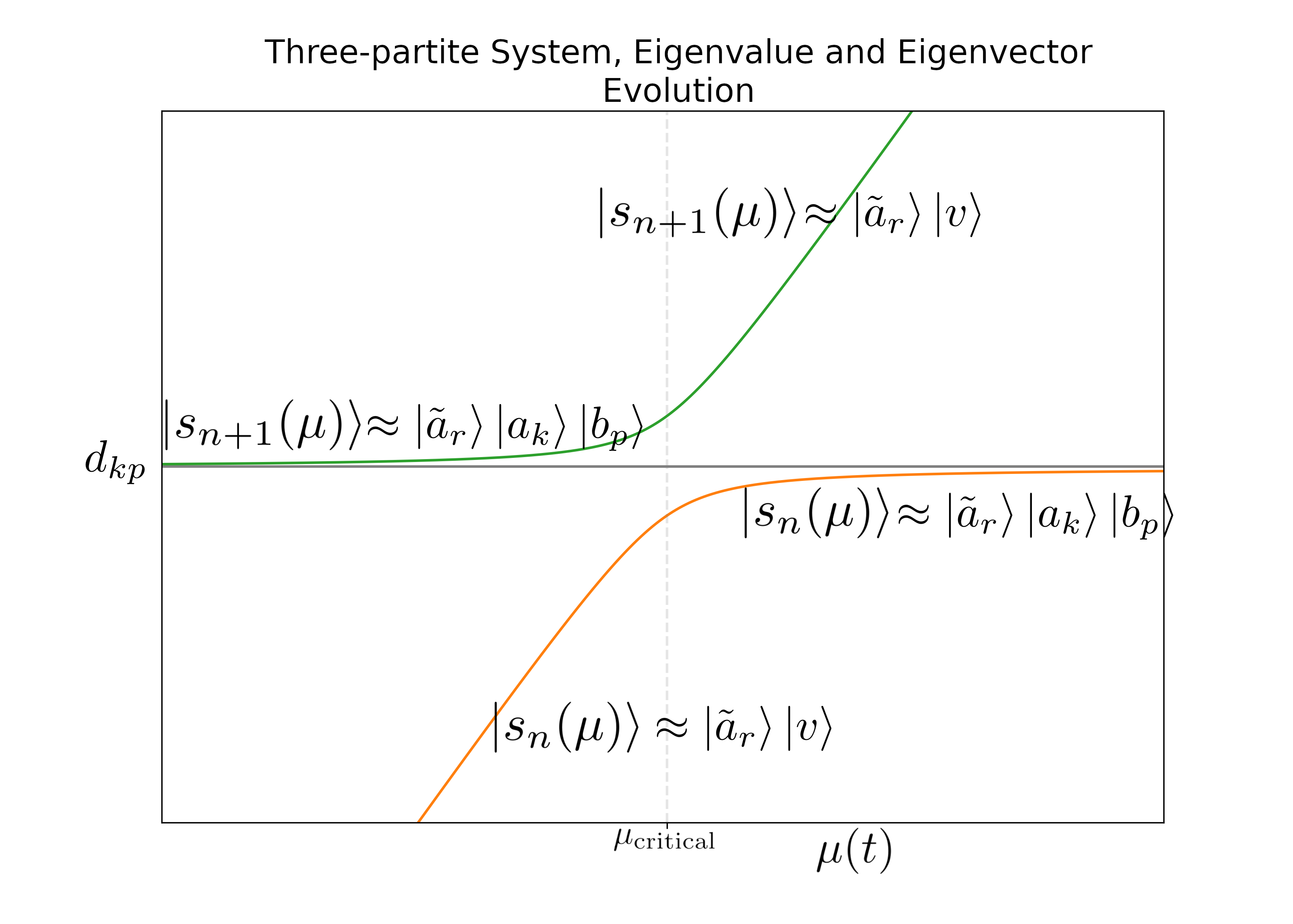
Figure 7: Example of an edge case in the three-partite system $\tilde{A}AB$. As two eigenvalues avoid a level crossing, they swap their eigenvectors, which can induce changes to the entanglement in system $\tilde{A}AB$.

where we can read off the basic dynamics of the entanglement in system $\tilde{A}AB$.

First, since the ancilla $\tilde{A}$ does not participate in the interaction, we obtain analogs of Observations 1 and 2 for system $AB$, if the ancilla $\tilde{A}$ is prepared unentangled. For example, since the result of any narrowly avoided level crossing is that the two eigenvalues swap their eigenvectors, any unentangled eigenstate of $D$, such as $|s_{n+1}(\mu)\rangle\approx|\tilde{a}_{r}\rangle|a_{k}\rangle|b_{p}\rangle$ ultimately evolves into another unentangled eigenstate of $D$, such as $|s_{n+1}(\mu)\rangle\approx|\tilde{a}_{r}\rangle|v\rangle$ and therefore no entanglement has been generated after an avoided level crossing. Except, during the brief period when the swap occurs, i.e., close to a critical $\mu$ value, an initially unentangled state such as here $|s_{n+1}(\mu)\rangle\approx|\tilde{a}_{r}\rangle|a_{k}\rangle|b_{p}\rangle$ will be a linear combination of the form: $|s_{n+1}(\mu)\rangle\approx\alpha|\tilde{a}_{r}\rangle|a_{k}\rangle|b_{p}\rangle+\beta|\tilde{a}_{r}\rangle|v\rangle$. We notice that if $|v\rangle\approx|a_{i}\rangle|b_{j}\rangle$ with $i\neq k$ and $j\neq p$, then $AB$ will be entangled around the critical $\mu$ value. As anticipated, since the ancilla is here a mere spectator, this matches 1 above for the bipartite case. Clearly, also 2 for the bipartite system $AB$ above has an immediate generalization to the tripartite system, if the ancilla system $\tilde{A}$ is chosen to be initially unentangled.

Finally, we analyze the fundamental processes in which an interaction induces a transfer of entanglement.

To this end, we assume that $\tilde{A}$ and $A$ are initially entangled and we use our findings above to study how an interaction between $A$ and $B$ can turn the initial entanglement between $\tilde{A}$ and $A$ into entanglement between $\tilde{A}$ and either $B$ or $AB$. Consider, for example, the initial state of the form

$$|\psi_{0}\rangle:=\frac{1}{\sqrt{2}}\left(|\tilde{a}_{r}\rangle|a_{k}\rangle|b_{p}\rangle+|\tilde{a}_{s}\rangle|a_{l}\rangle|b_{p}\rangle\right)$$ (2)

with $r\neq s$ and $k\neq l$. Here, systems $\tilde{A}$ and $A$ are entangled, and system $B$ is unentangled. Then, during the evolution, one of the two vectors on the RHS, say $|\tilde{a}_{r}\rangle|a_{k}\rangle|b_{p}\rangle$ will be the first to be swapped for $|v\rangle$ at some critical $\mu$ value. After passing this critical $\mu$ value, the initial state $|\psi_{0}\rangle$ will therefore have adiabatically evolved into:

$$|\psi_{1}\rangle:=\frac{1}{\sqrt{2}}\left(|\tilde{a}_{r}\rangle|v\rangle+|\tilde{a}_{s}\rangle|a_{l}\rangle|b_{p}\rangle\right)$$ (3)

We can now easily read off, for example, that by choosing $|v\rangle\approx|a_{l}\rangle|b_{q}\rangle$ with $q\neq p$, the state $|\psi_{1}\rangle$ possesses entanglement only between $\tilde{A}$ and $B$ while $A$ becoming unentangled:

$$|\psi_{1}\rangle\approx\frac{1}{\sqrt{2}}\left(|\tilde{a}_{r}\rangle|a_{l}\rangle|b_{q}\rangle+|\tilde{a}_{s}\rangle|a_{l}\rangle|b_{p}\rangle\right)$$ (4)

For this choice of $|v\rangle$, the interaction between $A$ and $B$, therefore, transferred the entanglement that $A$ initially possessed with $\tilde{A}$ to $B$, while passing the critical $\mu$ value.

Similarly, it is clear that the choice of $|v\rangle\approx|a_{t}\rangle|b_{q}\rangle$ with $t\neq l$ and $q\neq p$, transfers the entanglement that $\tilde{A}$ initially possessed with $A$ to system $AB$, by yielding instead the tri-partite entangled state:

$$|\psi_{1}\rangle\approx\frac{1}{\sqrt{2}}\left(|\tilde{a}_{r}\rangle|a_{t}\rangle|b_{q}\rangle+|\tilde{a}_{s}\rangle|a_{l}\rangle|b_{p}\rangle\right)$$ (5)

For this choice of $|v\rangle$, the interaction between $A$ and $B$ therefore transferred the entanglement that $A$ initially possessed with $\tilde{A}$ to the system $AB$.

Here, we only remark that, similarly, it is possible to systematically analyze the adiabatic dynamics of entanglement in $n$-partite systems with $n$ arbitrarily large.

III Mathematical preparations

As motivated above, we consider a time-dependent Hamiltonian that acts on an $N$-dimensional Hilbert space $\mathcal{H}$ and takes the form:

$$H_{tot}(t):=H_{0}+g(t)H_{int}$$ (6)

Here, $H_{0}$ and $H_{int}$ are Hermitian operators acting on $\mathcal{H}$. We refer to $H(0)=H_{0}$ as the initial Hamiltonian, and for some suitably chosen final time $T>0$, we call $H(T)$ the final Hamiltonian. The coupling function $g(t)$ is assumed to monotonically increase from $g(0)=0$ to a final value $g(T)$, slowly enough for the evolution to be adiabatic. As anticipated above, we break down this problem into more manageable parts. To this end, we invoke the spectral theorem and rewrite $H_{int}$ as a weighted sum of rank one projectors, $H_{int}=\sum_{k}\lambda_{k}\outerproduct{v_{k}}{v_{k}}$. Instead of adiabatically adding all of $g(T)H_{int}$ simultaneously to $H_{0}$, as in (6), we adiabatically add the weighted projectors $g(T)\lambda_{k}\outerproduct{v_{k}}{v_{k}}$ one by one to $H_{0}$.

Each activation of a projector is described by a time-dependent Hamiltonian of the form:

$$H(t):=D+\mu(t)\outerproduct{v}{v}$$ (7)

Here, for a fixed index $k$, we define $\outerproduct{v}{v}:=\outerproduct{v_{k}}{v_{k}}$. For the purpose of activating an individual projector, it is convenient to denote the starting and the final time of the activation of this new projector by $t=0$ and $t=t_{f}$, respectively. We choose $\mu(t)$ to be a function that monotonically runs from $\mu(0)=0$ to $\mu(t_{f})=g(T)\lambda_{k}$ slowly enough for the evolution to be adiabatic. We now focus on the dynamics during the addition of an individual projector.

Before we get to the main results, we present a useful lemma which shows that for an eigenvalue $s$, there is an eigenstate $\ket{s}$ of the Hamiltonian $H(t)$ in (7) for which nonperturbatively an explicit expression can be given.

Lemma 1.

Let $H(t)$ in (7) be the Hamiltonian of a quantum system with a non-degenerate spectrum. Let $\ket{v}$ be arbitrary. For any eigenvalue $s:=s(\mu(t))$ of $H(t)$, the corresponding eigenstate $\ket{s}$ is given by

$$\ket{s} =\gamma\big{(}sI-D\big{)}^{-1}\ket{v},$$ (8)

where $\gamma$ is a normalization constant defined as

$$\gamma=\frac{1}{\|(sI-D)^{-1}\ket{v}\|}.$$ (9)

The lemma states that the eigenstate $\ket{s}$ can be explicitly expressed as a function of $\ket{v}$, the initial Hamiltonian $D$, and the eigenvalue $s$. The proof of this lemma and of the subsequent propositions in this paper are in the appendices.

The lemma can be combined with the adiabatic theorem [1, 3], which says that if a quantum system is initialized in an eigenstate of the initial Hamiltonian $D$ and evolved sufficiently slowly, then, for any time $t$, the system’s state will stay arbitrarily close to an instantaneous eigenstate of $H(t)$ corresponding to the same energy level.

Lemma 2.

Let $H(t)$ in (7) be the Hamiltonian of a quantum system whose spectrum is non-degenerate, and let $\ket{v}$ be arbitrary. Let $u:=t/t_{f}\in[0,1]$ and $\tilde{\mu}(u):=\mu(ut_{f})$, then the rescaled version of $H(t)$ is:

$$\tilde{H}(u):=D+\tilde{\mu}(u)\outerproduct{v}{v}$$ (10)

Assume that the system is initially in the $n$’th–level energy eigenstate $\ket{\tilde{s}_{n}(0)}=\ket{d_{n}}$ of $\tilde{H}(0)=D$. Suppose that it undergoes adiabatic evolution until a final time $t_{f}$, which is chosen in accordance with the condition of the adiabatic theorem [3]:

$$t_{f} \gg\max_{u\in[0,1]}\frac{\left|\innerproduct{\tilde{s}_{m}(u)}{v}\innerproduct{v}{\tilde{s}_{n}(u)}d\tilde{\mu}/du\right|}{\tilde{s}_{nm}(u)^{2}},\ \ \ n\neq m$$ (11)

Here, $\tilde{s}_{nm}(u)=\tilde{s}_{n}(u)-\tilde{s}_{m}(u)$ and $\tilde{s}_{k}(u)$ is an eigenvalue of $\tilde{H}(u)$. Then, the evolved state of the system at time $t_{f}$ will in effect remain in the instantaneous eigenstate $\ket{s_{n}(\mu(t_{f}))}$, that is

$$\left\|U(t_{f})\ket{d_{n}}-\ket{s_{n}(\mu(t_{f}))}\right\|\approx 0,$$ (12)

where

$$U(t_{f}) :=\mathcal{T}\exp\left\{-\textrm{i}\int_{0}^{t_{f}}H(t)dt\right\},$$ (13)

and $\mathcal{T}$ denotes the time-ordering operator. In the limit of $t_{f}\rightarrow\infty$, we have the exact relation:

$$U(t_{f})\ket{d_{n}}=\ket{s_{n}(\mu(t_{f}))}=\gamma(s_{n}(\mu(t_{f}))I-D)^{-1}\ket{v}$$ (14)

In this paper, we always assume that $t_{f}$ is chosen sufficiently large to ensure that the time evolution operator $U(t_{f})$ evolves the initial eigenstate $\ket{d_{n}}$ into the eigenstate $\ket{s_{n}(t_{f})}$ to any desired target accuracy, so that, in effect, we can write $U(t_{f})\ket{d_{n}}=\ket{s_{n}(t_{f})}$.

Remark: The reason for using the unitless variable $u$ in condition (11) traces to the observation that traditional conditions for adiabaticity had missed the fact that exceptional non-adiabaticity can build up through resonances from seemingly adiabatic oscillatory time dependence in the Hamiltonian, see [3]. The condition that the Hamiltonian can be written as a function of the unitless time variable $u$ excludes such oscillatory behaviour because it would set a new scale. This, in turn, renders condition (11) robust. For a detailed review, see [5].

III.1 The relationship between the coupling strength $\mu(t_{f})$ and the final eigenvalue $s$.

It would be desirable to be able to express the eigenvalues, $s_{n}(\mu)$ of a Hamiltonian $H(\mu)=D+\mu|v\rangle\langle v|$ as an explicit expression in radicals, e.g., by solving explicitly for the roots, $s_{n}(\mu)$, of the characteristic polynomial of $H(\mu)$. As Galois theory showed, this is impossible for Hilbert space dimensions larger than 4, see [9]. In this section, we present a lemma, see also [8], that describes a method to bypass this limitation by inverting the problem: it is possible to give an explicit expression for $\mu$ as a function of the eigenvalue $s$ for all real $s$. Concretely, working in the eigenbasis $\{\ket{d_{k}}\}_{k=0}^{N-1}$ of the initial Hamiltonian $D$, we have:

$$\mu(s)=\left(\sum_{k=0}^{N-1}\frac{|v_{k}|^{2}}{s-d_{k}}\right)^{-1}$$ (15)

In the equation above, $v_{k}:=\innerproduct{v}{d_{k}}$ and the $d_{k}$ are the eigenvalues of the initial Hamiltonian $D$.

Therefore, one can fix $s$ and then use (15) to obtain the desired coupling strength $\mu$ so that $H(\mu)$ has $s$ as an eigenvalue.

Lemma 3.

Let $s$ be an arbitrary real number. Consider the Hamiltonian defined by $H(s)=D+\mu(s)\outerproduct{v}{v}$, where $\mu(s)$ is as in (15) and $\ket{v}$ is arbitrary. Then, $s$ is an eigenvalue of $H(s)$.

Allowing $s$ to change over time, we will, for simplicity, write $H(t)=H(s(t))$. Incorporating the principles from Lemma 2 and Lemma 3, a comprehensive non-perturbative framework can be formulated for the determination of final eigenstates and eigenvalues of a time-dependent Hamiltonian $H(t)$. Initially, one selects a real number $s$ and employs Lemma 3 to define the final Hamiltonian $H(t_{f})$. Subsequently, Lemma 1 provides the exact form of the final eigenstate associated with $H(t_{f})$.

In instances where pre-selecting the eigenvalue $s$ is impractical, an alternative strategy is to establish a fixed value for $\mu(t_{f})$ and then employ numerical methods in conjunction with (15).

IV Transmission and Preservation of Entanglement in Tripartite Systems

In this section, our goal is to identify the elementary principles that govern entanglement transmission or preservation under addition of the initial Hamiltonian $D$ and the coupling term $\mu(t)\outerproduct{v}{v}$. Therefore, we investigate the dynamics of entanglement within a tri-partite system situated in the Hilbert space $\mathcal{H}_{\tilde{A}}\otimes\mathcal{H}_{A}\otimes\mathcal{H}_{B}$. We assume here that system $A$ is initially prepared entangled with an ancillary system $\tilde{A}$, such that $\tilde{A}$ purifies $A$. The system $B$ is assumed to be initially pure and unentangled with both $A$ and $\tilde{A}$. Subjected to a time-dependent Hamiltonian as in (16), the composite pure system $\tilde{A}AB$ then undergoes adiabatic evolution while $\tilde{A}$ remains inert. The interaction between $A$ and $B$ induced by the term $\mu(t)\outerproduct{v}{v}$ can then not only entangle the systems $A$ and $B$ but can also transfer entanglement that $A$ initially possessed with $\tilde{A}$ to $B$ or $AB$. The setup is illustrated in Figure 1. For example, $\tilde{A}$ and $A$ might represent qubits in a quantum processor, while $B$ could describe another qubit of the processor or an environment.

We assume that the following Hamiltonian interaction governs the adiabatic evolution:

$$H(t)=I\otimes H_{A}\otimes I+I\otimes I\otimes H_{B}+\mu(t)I\otimes\outerproduct{v}{v}$$ (16)

Here, $H_{A}$ and $H_{B}$ denote the Hamiltonians of systems $A$ and $B$ respectively. We define the initial Hamiltonian $D$ as $D:=H_{A}\otimes I+I\otimes H_{B}$. Subsequently, the total Hamiltonian in (16) simplifies to:

$$H(t)=I\otimes D+\mu(t)I\otimes\outerproduct{v}{v}$$ (17)

For this system, let $\{\ket{a_{i}}\}$ and $\{\ket{b_{i}}\}$ represent the sets of eigenstates corresponding to systems $A$ and $B$ respectively. Additionally, we introduce $\{\ket{\tilde{a}_{i}}\}$ as an arbitrary basis for the ancillary system $\tilde{A}$. We let the system $\tilde{A}A$ start in a pure state. For some fixed $i$ and $j$, we define the state of $\tilde{A}A$ to be

$$\ket{\psi_{\tilde{A}A}}=\alpha_{ii}\ket{\tilde{a}_{i}}\ket{a_{i}}+\alpha_{jj}\ket{\tilde{a}_{j}}\ket{a_{j}},$$ (18)

where $\alpha_{ii}$ and $\alpha_{jj}$ are complex coefficients. We may assume, for example, an entangled state $\ket{\psi_{\tilde{A}A}}$ with $|\alpha_{ii}|^{2}=|\alpha_{jj}|^{2}=1/\sqrt{2}$. Then the joint initial state of $\tilde{A}AB$ is:

$$\ket{\psi_{\tilde{A}AB}}=\left(\alpha_{ii}\ket{\tilde{a}_{i}}\ket{a_{i}}+\alpha_{jj}\ket{\tilde{a}_{j}}\ket{a_{j}}\right)\ket{b_{0}}$$ (19)

Now, we are ready to establish the conditions for maximizing the transfer or preservation of entanglement during the course of adiabatic evolution. That is, we show that for an appropriate choice of $\ket{v}$ and $\mu(t_{f})$, it is possible to transmit entanglement in the sense that $\tilde{A}$’s initial entanglement with $A$ turns into entanglement of $\tilde{A}$ with $B$, while $A$ becomes pure and therefore disentangled from both $\tilde{A}$ and $B$. Conversely, we show how to reverse the entanglement transmission so that $\tilde{A}$ is again entangled with $A$, and $B$ returns to being in a pure state.

Furthermore, we find that transferring entanglement is computationally expensive due to the need for a slower rate of adiabatic evolution. As we will discuss in Section VII, selecting the state $\ket{v}$ to maximize entanglement transfer leads to reduced energy gaps of the Hamiltonian in (16), which is important because the minimum duration, $t_{f}$, of the evolution is determined by the minimum energy gap, see, e.g., (11). We find that highly efficient entanglement transfer necessitates a significantly prolonged evolution time.

Another interesting finding is that entanglement transfer and preservation are not continuous processes. We show that entanglement relations between systems can abruptly reverse to their original state even if $\mu(t_{f})$ and $\ket{v}$ are changed in a continuous manner.

Let us first start with the trivial choice of $\ket{v}$. Let $\ket{v}$ be an eigenstate of the Hamiltonian $D=H_{A}\otimes I+I\otimes H_{B}$. That is, $\ket{v}=\ket{a_{p}}\ket{b_{k}}$ for some fixed $p$ and $k$. In this case, the initial Hamiltonian $I\otimes D$ commutes with the interaction Hamiltonian $\mu(t)I\otimes\outerproduct{v}{v}$ and the final state $\ket{\psi_{\tilde{A}^{\prime}A^{\prime}B^{\prime}}}$ only acquires relative phases:

$$\ket{\psi_{\tilde{A}^{\prime}A^{\prime}B^{\prime}}}=\alpha_{ii}\omega_{ii}\ket{\tilde{a}_{i}}\ket{a_{i}}\ket{b_{0}}+\alpha_{jj}\omega_{jj}\ket{\tilde{a}_{j}}\ket{a_{j}}\ket{b_{0}}$$ (20)

where $|\omega_{ii}|,|\omega_{jj}|=1$ for some fixed $i$ and $j$. Importantly, $\tilde{A}A$ remains entangled and pure, and $B$ is unentangled and pure. Therefore, the entanglement structure remained unchanged. In this trivial case, we see that $\ket{v}$, being an eigenstate of $D$, cannot affect the entanglement characteristics of any of the systems.

It is reasonable to assume that $\ket{v}$ that maximizes the transmission or preservation of entanglement must be a linear combination of specific eigenstates of $D$. Indeed, this is the case. However, surprisingly, such $\ket{v}$ must be arbitrarily close to exactly one of the eigenstates of $D$ and yet not be equal to it. Using the notation $\mu_{t_{f}}$ to represent $\mu(t_{f})$ and defining $v_{kp}$ as the coefficients of $\ket{v}$ in the eigenbasis $\{\ket{a_{k}}\ket{b_{p}}\}_{kp}$, where

$$v_{kp}=\innerproduct{v}{a_{k}b_{p}},$$ (21)

we present the following theorem.

Theorem 4.

Let $n=\dim A$ and $m=\dim B$. For some fixed indices $i<j$, suppose the eigenvalues of $D$ are ordered as

$$d_{i0}<d_{i1}<\cdots<d_{j0}<d_{j1}.$$ (22)

Let system $\tilde{A}A$ be entangled and $B$ be in a pure, unentangled state:

$$\ket{\psi_{\tilde{A}AB}}=\alpha_{ii}\ket{\tilde{a}_{i}}\ket{a_{i}}\ket{b_{0}}+\alpha_{jj}\ket{\tilde{a}_{j}}\ket{a_{j}}\ket{b_{0}}$$ (23)

Fix an index $\ell\geq 0$ such that $d_{i0}\leq d_{i\ell}<d_{j0}$. For $\epsilon>0$, if $\ket{v}$ is such that

$$v_{kp}=\begin{cases}1-(nm-1)\epsilon^{2}&\text{for }k=i,p=\ell,\\ \epsilon&\text{otherwise},\end{cases}$$ (24)

and

$$\mu_{t_{f}}\in\left(\frac{d_{j0}-d_{i\ell}}{|v_{i\ell}|^{2}},\frac{d_{j1}-d_{i\ell}}{|v_{i\ell}|^{2}}\right).$$ (25)

Then, as $\epsilon\to 0$, the entanglement of the evolved system is such that $\tilde{A}$ becomes entangled with $B$, and $A$ becomes pure and unentangled. Furthermore, if

$$\mu_{t_{f}}>\frac{d_{j1}-d_{i\ell}}{|v_{i\ell}|^{2}},$$ (26)

then as $\epsilon\to 0$, the entanglement of the evolved system is such that $\tilde{A}$ becomes again entangled with $A$, and $B$ becomes again pure and unentangled.

The theorem, therefore, provides us with a construction of interaction Hamiltonians $\mu(t_{f})\outerproduct{v}{v}$ to accomplish transfer or preservation of entanglement. Furthermore, the theorem explicitly identifies the values of $\mu(t_{f})$ at which $A$ transfers its entanglement with $\tilde{A}$ to $B$, as detailed in (25). It also specifies the precise values of $\mu(t_{f})$ required to revert the entanglement relationships back to their original configuration.

We note that since $\ket{v}$ in (24) has the dominant component $v_{i\ell}\approx 1$ for $\epsilon\ll 1$, it is close to an eigenstate $\ket{a_{i}}\ket{b_{\ell}}$ of the initial Hamiltonian $D$. However, $\ket{v}$ significantly differs from $\ket{a_{i}}\ket{b_{\ell}}$ in its effect on the final system’s entanglement structure. We see that entanglement transfer or preservation is not continuous relative to the change of $\ket{v}$. For example, one might construct $\ket{v}$ with sufficiently small $\epsilon$ and some finite $\mu_{t_{f}}$ such that $\tilde{A}$ becomes entangled with $B$ and $A$ becomes pure and unentangled. However, if $\epsilon$ reaches its limit $0$, i.e., $\epsilon=0$, then $\ket{v}=\ket{a_{i}}\ket{b_{\ell}}$ and the structure of entanglement abruptly reverts to its original state. This is because, as we have seen, eigenstates of $D$ do not change the entanglement structure of the initial system, i.e., $A$ remains entangled with $\tilde{A}$ and $B$ remains pure and unentangled.

V Entanglement Transfer/Preservation Induces Structured Eigenspectrum and Eigenvector Dynamics.

The dynamics of eigenvalues and associated eigenstates of $H(t_{f})$, under the influence of $\mu(t_{f})\outerproduct{v}{v}$ as constructed in Theorem 4, play a crucial role in understanding entanglement transfer and preservation in quantum systems. In this section, we explore these dynamics in detail, showing that each eigenstate of the initial Hamiltonian $D$ undergoes a three-stage adiabatic evolution.

Initially, in the first stage of the evolution, an eigenstate of $D$ remains nearly static, exhibiting minimal change. The second stage is marked by the eigenstate closely aligning with $\ket{v}$, reflecting a significant shift in its characteristics. Finally, in the third stage, the eigenstate transitions towards a neighbouring higher energy eigenstate. Similar behaviour can be observed for the eigenvalues. Each eigenvalue undergoes exactly the same three-stage evolution. In the first state, an eigenvalue remains almost static. During the second stage, the eigenvalue increases at a speed close to $1$. Importantly, only one eigenvalue at a time has a velocity near $1$ while the rest remain almost static. During the third stage, the eigenvalue approaches a higher energy eigenvalue and slows down without ever crossing it. The dynamics of this behaviour are illustrated in Figure 3. This three-stage progression elucidates the mechanisms behind the subtle shifts in eigenstate positions and energies, providing a comprehensive understanding of how entanglement properties are influenced and manipulated through the choice of $\mu(t_{f})\outerproduct{v}{v}$ in Theorem 4.

The influence of positive semidefinite $\mu(t_{f})\outerproduct{v}{v}$ with an arbitrary $\ket{v}$ is thoroughly documented in the literature [8, 10]. Generally, the neighbouring eigenvalues $s_{k}<s_{k+1}$ of $H(t_{f})$ interlace with the neighbouring eigenvalues $d_{k}<d_{k+1}$ of $D$. This yields the interlacing inequality:

$$d_{k}\leq s_{k}\leq d_{k+1}\leq s_{k+1}$$ (27)

As $\mu_{t_{f}}$ increases from negative infinity to positive infinity, the eigenvalues of $H(t_{f})$ increase monotonically. Absence of orthogonality between $\ket{v}$ and any eigenstate $\ket{d_{k}}$ of $D$ ensures the prohibition of energy level-crossings for all finite $\mu_{t_{f}}$. Conversely, if $\ket{v}$ is orthogonal to a particular eigenstate $\ket{d_{j}}$, then the associated eigenvalue $s_{j}$ remains fixed, permitting potential level-crossings. This scenario has been previously encountered in Section IV; when $\ket{v}$ coincided with an eigenvector of $D$. In this scenario, when $\mu_{t_{f}}$ approaches positive infinity, a single eigenvalue increases, sequentially crossing all higher energy levels. Furthermore, we have seen that such $\ket{v}$ does not change the entanglement structure for any values of $\mu_{t_{f}}$.

On the other hand, the optimal selection of $\ket{v}$ in Theorem 4 maximizes entanglement transmission or preservation for finite values $\mu_{t_{f}}$, it also imposes a strict pattern in the evolution of eigenvalues $s_{k}$ and eigenstates $\ket{s_{k}}$ of $H(t)$. As per the formulation of $\ket{v}$ in (24) with $\epsilon>0$ sufficiently small, no level-crossings occur for all finite $\mu_{t_{f}}$ due to the non-zero components $v_{k}=\innerproduct{v}{d_{k}}\geq\epsilon$ with any eigenstate $\ket{d_{k}}$ of $D$. Furthermore, considering the eigenvalue velocities total to unity [8, 10], at any moment, precisely one eigenvalue exhibits a velocity of $|1-(nm-1)\epsilon^{2}|^{2}\approx 1$, with the rest advancing minimally with the maximum velocity proportional to $\epsilon^{2}\approx 0$. Specifically, as $\mu_{t_{f}}$ increases, a solitary eigenvalue $s_{k}$ ascends to the next larger eigenvalue $s_{k+1}$ at a velocity of $|1-(nm-1)\epsilon^{2}|^{2}$. Due to the eigenvalue $s_{k}$ ascending to the almost static larger eigenvalue $s_{k+1}$, the energy gap becomes narrower, yet no level-crossing is happening. The level-crossing avoidance can be attributed to an eventual deceleration in eigenvalue velocity which changes from $|1-(nm-1)\epsilon^{2}|^{2}$ to near zero, and the larger eigenvalue $s_{k+1}$ acquiring the velocity of $|1-(nm-1)\epsilon^{2}|^{2}$ and hence avoiding the crossing with the eigenvalue $s_{k}$.

Consequently, we can categorize the behaviour of each eigenvalue $s_{k}$ of $H(t)$ and its corresponding eigenvector into three distinct evolutionary phases, characterized by three specific intervals of $\mu(t)$. During the initial interval $\mathcal{I}_{1}:=(-\infty,\mu_{1})$, the eigenvalue $s_{k}$ is $\epsilon^{2}$–close to $d_{k}$ with the maximum velocity proportional to $\epsilon^{2}$. In the subsequent interval $\mathcal{I}_{2}:=(\mu_{1},\mu_{2})$, the eigenvalue $s_{k}$ experiences an increased velocity of $|1-(nm-1)\epsilon^{2}|^{2}$, indicating a more rapid ascent. Finally, in the interval $\mathcal{I}_{3}:=(\mu_{2},+\infty)$, the eigenvalue $s_{k}$ is $\epsilon^{2}$–close to $d_{k+1}$ and resumes back to a slower pace. These intervals collectively span nearly the entire spectrum of the real line. This comprehensive coverage allows us to predict the eigenstate $\ket{s_{k}}$ associated with any given value of $\mu(t)$ within these intervals. This observation is formally presented in the following theorem.

Theorem 5.

Let $N$ be the dimension of the Hilbert space that $H(t)$ acts on and $\{d_{j}\}_{j=0}^{N-1}$ be the increasing sequence of the eigenvalues of $D$.

Fix index $i$ and let $\epsilon>0$. Suppose $\ket{v}$ is a vector characterized by its components $v_{j}=\innerproduct{v}{d_{j}}$ as follows:

$$v_{j}=\begin{cases}1-(N-1)\epsilon^{2}&\text{if }j=i\\ \epsilon&\text{otherwise}\end{cases}$$ (28)

For $k>i$, if $\mu_{t_{f}}$ lies within the interval

$$\left(-\infty,\frac{d_{k}-d_{i}}{|v_{i}|^{2}}\right),$$ (29)

then the eigenstate $\ket{d_{k}}$ of $D$ adiabatically evolves as

$$U_{t_{f}}\ket{d_{k}}\rightarrow\ket{d_{k}}\text{ as }\epsilon\rightarrow 0.$$ (30)

If $\mu_{t_{f}}$ lies within the interval

$$\left(\frac{d_{k}-d_{i}}{|v_{i}|^{2}},\frac{d_{k+1}-d_{i}}{|v_{i}|^{2}}\right),$$ (31)

then

$$U_{t_{f}}\ket{d_{k}}\rightarrow\ket{d_{i}}\text{ as }\epsilon\rightarrow 0.$$ (32)

If $\mu_{t_{f}}$ lies within the interval

$$\left(\frac{d_{k+1}-d_{i}}{|v_{i}|^{2}},+\infty\right),$$ (33)

then

$$U_{t_{f}}\ket{d_{k}}\rightarrow\ket{d_{k+1}}\text{ as }\epsilon\rightarrow 0.$$ (34)

The endpoints of the interval in (31) deserve special attention. These are the “critical points” around which eigenstate transitions are happening. For $\epsilon$ sufficiently small, consider the critical point $\mu_{k+1}:=(d_{k+1}-d_{i})/|v_{i}|^{2}$ in (31). Slightly before this critical point, say at $\mu_{k+1}-\Delta\mu$, the state $\ket{d_{k}}$ evolves into $\ket{d_{i}}$. However, right after the critical point at $\mu_{k+1}+\Delta\mu$, the state $\ket{d_{k}}$ evolves into the next energy level eigenstate $\ket{d_{k+1}}$, while the state $\ket{d_{k+1}}$ evolves into $\ket{d_{i}}\approx\ket{v}$. Essentially, in the limit of $\epsilon$ tending to zero, this evolution behaviour can be characterized as a swap: $\ket{d_{k}}$ and $\ket{d_{k+1}}$ swap places while $\mu(t)$ passes the critical point. To emphasize this remarkable fact, we present an alternative theorem that focuses on the eigenstate transitions around the critical points.

Theorem 6 (Alternative).

Let $\{d_{j}\}_{j=0}^{N-1}$ be an increasing sequence of eigenvalues of $D$.

Fix index $i$ and let $\epsilon\in(0,1)$. Suppose $\ket{v}$ is a vector characterized by its components $v_{j}=\innerproduct{v}{d_{j}}$ as follows:

$$v_{j}=\begin{cases}1-(N-1)\epsilon^{2}&\text{if }j=i\\ \epsilon&\text{otherwise}\end{cases}$$ (35)

For each $k\geq i$, define $\mu_{k+1}$ as:

$$\mu_{k+1}:=\frac{d_{k+1}-d_{i}}{|v_{i}|^{2}}$$ (36)

Let $U(t)$ be the adiabatic evolution operator of $H(t)$. Then, in the limit as $\epsilon\to 0$, the following transitions occur:

$$U\left(t(\mu_{k+1}-\Delta\mu)\right)\ket{d_{k}}\rightarrow\ket{d_{i}}$$ (37)

$$U\left(t(\mu_{k+1}+\Delta\mu)\right)\ket{d_{k}}\rightarrow\ket{d_{k+1}}$$ (38)

$$U\left(t(\mu_{k+1}-\Delta\mu)\right)\ket{d_{k+1}}\rightarrow\ket{d_{k+1}}$$ (39)

$$U\left(t(\mu_{k+1}+\Delta\mu)\right)\ket{d_{k+1}}\rightarrow\ket{d_{i}}$$ (40)

In the above, $\Delta\mu$ is chosen such that

$$0<\Delta\mu<\min\{\mu_{k+2}-\mu_{k+1},\mu_{k+1}-\mu_{k}\},$$ (41)

where $\mu_{k}<\mu_{k+1}<\mu_{k+2}$.

Theorem 5 and its alternative formulation Theorem 6 illustrate explicit dynamics of eigenstate transitions around the critical points $\mu_{\text{critical}}\equiv\mu_{k}$. Both theorems can be further conceptualized in a succinct statement which describes a swap of states around the critical points. To get an intuition for the upcoming statements, it is useful to examine Figure 5 where we see the mechanics of a swap. Specifically, for $\mu<\mu_{\text{critical}}$, the eigenstate $\ket{s_{k}(\mu)}\approx\ket{v}$, whereas $\ket{s_{k+1}(\mu)}\approx\ket{d_{k+1}}$. However, for $\mu>\mu_{\text{critical}}$, we have $\ket{s_{k}(\mu)}\approx\ket{d_{k+1}}$ and $\ket{s_{k+1}(\mu)}\approx\ket{v}$.

Theorem 7 (Eigenstates Swap).

Let $d_{k+1}$ be an eigenvalue of $D$. Suppose that $\ket{v}$ is constructed as in (35). Let $\mu_{k+1}$ and $\Delta\mu>0$ be the critical point and increment of $\mu_{k+1}$ as described in (36) and (41), respectively. Then, in the limit $\epsilon\rightarrow 0$, we have the following relation:

$$\ket{s_{k}(\mu_{k+1}-\Delta\mu)}=\ket{v}\ \text{ and }\ \ket{s_{k+1}(\mu_{k+1}-\Delta\mu)}=\ket{d_{k+1}}$$

$$\ket{s_{k}(\mu_{k+1}+\Delta\mu)}=\ket{d_{k+1}}\ \text{ and }\ \ket{s_{k+1}(\mu_{k+1}+\Delta\mu)}=\ket{v}$$

Here, for the adiabatic evolution operator $U(t(\mu))$ of $H(t)$, we have:

$$\ket{s_{k}(\mu)}:=U(t(\mu))\ket{d_{k}}$$ (42)

VI Group theoretic view of the special construction of $\ket{v}$

In the previous section, we showed that the evolution with $\ket{v}$ constructed as in Theorem 7 results in two eigenvalues swapping their eigenvectors. It is possible to represent this swapping as a transposition of two elements in a set comprised of eigenvectors of $H(t)$. A transposition in a set of elements is a permutation that exchanges two elements and keeps all the rest unchanged.

It is well known that the permutation group $S_{N}$ on $N$ elements can be generated by composing transpositions. This means that using multiple interaction terms, which are constructed according to Theorem 7, we can obtain any permutation of eigenvectors of the Hamiltonian $H(t)$. By this, we mean that upon addition of the specially constructed interaction terms $\mu^{(j)}(t)|v^{(j)}\rangle\langle v^{(j)}|$ to the initial Hamiltonian $D$, the eigenvalues of $H(t)=D+\sum_{j}\mu^{(j)}(t)|v^{(j)}\rangle\langle v^{(j)}|$ will have the eigenvectors of the initial Hamiltonian $D$ but permuted. To see this remarkable relation, consider the Hamiltonian

$$H(t)=D+\mu(t)\outerproduct{v}{v},$$ (43)

where $\mu(0)=0$. Let

$$M_{0}:=\{\ket{d_{0}},\ket{d_{1}},\ldots,\ket{d_{k}},\ldots,\ket{d_{N-1}}\}$$ (44)

denote an ordered set of eigenvectors of $H(0)=D$ with the corresponding eigenvalues ordered as

$$d_{0}<d_{1}<\cdots<d_{k}<\cdots<d_{N-1}.$$ (45)

We now construct $\ket{v}$ in accordance with Theorem 7. Specifically, we set the $k$th component of $\ket{v}$ to be dominant, $v_{k}=1-(N-1)\epsilon^{2}$ where $\epsilon\ll 1$. The rest of the components are set to $\epsilon$. Let $t_{f}$ denote the final time. Set $\mu(t_{f})=\mu_{k+1}+\Delta\mu$ where $\mu_{k+1}$ is the critical $\mu$-value defined as

$$\mu_{k+1}=\frac{d_{k+1}-d_{k}}{|v_{k}|^{2}},$$ (46)

and $0<\Delta\mu<\mu_{k+2}$.

By Theorem 7, in the limit $\epsilon\rightarrow 0$, the final Hamiltonian $H(t_{f})$ will have the following ordered set of eigenvectors

$$M_{t_{f}}=\{\ket{d_{0}},\ket{d_{1}},\ldots,\ket{d_{k+1}},\ket{d_{k}},\ldots,\ket{d_{N-1}}\},$$ (47)

with the corresponding eigenvalues

$$s_{0}<s_{1}<\cdots<s_{k}<s_{k+1}<\cdots<s_{N-1}.$$ (48)

We note that the final Hamiltonian $H(t_{f})$ has the same eigenvectors as the initial Hamiltonian $H(0)=D$, but the $k$th and $k+1$ eigenvalues have traded eigenvectors, i.e., the eigenvalues $s_{k}<s_{k+1}$ have the associated eigenvectors $\ket{d_{k+1}}$ and $\ket{d_{k}}$, respectively. We have illustrated this behaviour in Figure 5.

In the construction above, we have shown that choosing the $k$th component of $\ket{v}$ to be dominant and choosing the critical point $\mu_{k+1}$ accomplishes the transposition of eigenvectors $\ket{d_{k}}$ and $\ket{d_{k+1}}$. Using the group theoretic cycle notation, we let $(k,k+1)$ denote a transposition of elements $k$ and $k+1$, and $*$ denote the action of transposition on a set of elements. For example, $(3,4)*\{1,2,3,4\}=\{1,2,4,3\}$ signifies that $3$ is mapped to $4$, and $4$ is mapped to $3$. Therefore, the choice of the dominant component $v_{k}$ and the critical point $\mu_{k+1}$ can be succinctly represented as a transposition $(k,k+1)$ which acts on a set of eigenvectors $M_{0}$. Hence, we can write

$$(k,k+1)*M_{0}=M_{t_{f}}.$$ (49)

It is now trivial to see how adding multiple rank-one projectors affects the eigenstates of $H(t)$. Let $D^{(1)}:=H(t_{f})$ and add another interaction term $\mu^{(2)}(t)|v^{(2)}\rangle\langle v^{(2)}|$ such that $\mu^{(2)}(t)=0$ for $t\leq t_{f}$. Then, the updated Hamiltonian is

$$H(t) =D^{(1)}+\mu^{(2)}(t)|v^{(2)}\rangle\langle v^{(2)}|,$$ (50)

such that

$$H(t) =D^{(1)},\text{ for }t=t_{f},$$ (51)

$$H(t) =D^{(1)}+\mu^{(2)}(t)|v^{(2)}\rangle\langle v^{(2)}|,\text{ for }t_{f}<t\leq t_{f}^{(2)}.$$ (52)

We, construct $|v^{(2)}\rangle$ with a dominant component $v^{(2)}_{j}$, choose the critical point $\mu_{j+1}^{(2)}$ and let $\mu(t_{f}^{(2)})=\mu_{j+1}^{(2)}+\Delta\mu^{(2)}$. Using the cyclic notation for transposition, we can easily obtain the set $M_{t_{f}^{(2)}}$ of eigenvectors of $H(t_{f}^{(2)})$. To this end, perform the following computation:

$$(j,j+1)(k,k+1)*M_{0}=(j,j+1)*M_{t_{f}}=M_{t_{f}^{(2)}}$$ (53)

That is, we first swap elements $k$ and $k+1$, and then we swap elements ${j,j+1}$.

This abstraction allows us to deduce several interesting properties about the addition of specially constructed rank-one projectors. For example, if $\mu^{(2)}(t)|v^{(2)}\rangle\langle v^{(2)}|$ is introduced before $\mu(t)\outerproduct{v}{v}$, how does the ordering of eigenstates change? We can easily answer this question by recalling that the transpositions $(j,j+1)$ and $(k,k+1)$ commute if $j\neq k$. Therefore, the ordering of eigenvectors of the final Hamiltonian $H(t_{f}^{(2)})$ is the same regardless of which interaction term is introduced first as long as $j\neq k$.

Recalling that transpositions generate the permutation group $S_{N}$, we can deduce that adding multiple specially constructed rank-one projectors is equivalent to composing transpositions, and by composing transpositions, we can achieve any permutation. Therefore, it is possible to induce any ordering of eigenstates of the final Hamiltonian.

We would like to point out that transpositions are not the only types of permutation that can be achieved. It is also possible to choose the critical point $\mu_{k}$ such that the associated permutation is a shift. To see this, choose the dominant component to be $v_{k}$ for $k<N-1$. Then choose the critical point $\mu_{N-1}$ and set $\mu(t_{f})=\mu_{N-1}+\Delta\mu$. Then, the associated permutation is a shift to the right of all elements that are greater or equal to $k$. This shift in cycle notation is $(k,k+1,k+2,\ldots,N-1)$. The rest of the elements remain unchanged.

Since the set of permutations $S_{N}$ forms a group, it contains a neutral element, and each element in $S_{N}$ has an inverse. We can identify the neutral element of $S_{N}$ with the interaction term $\mu(t)\outerproduct{v}{v}$ where $\ket{v}$ is simply an eigenvector of $D$. Adding such an interaction term will keep the order of eigenvectors unchanged. To find the inverse of a permutation, it is sufficient to identify inverses of transpositions $(k,k+1)$. In other words, we want to find $\mu^{(2)}(t)|v^{(2)}\rangle\langle v^{(2)}|$, which reverses the action of $\mu(t)\outerproduct{v}{v}$ associated with the transposition $(k,k+1)$. To achieve this, we work in the eigenbasis of $D^{(1)}=D+\mu(t_{f})\outerproduct{v}{v}$. Next, we choose a critical point $\mu^{(2)}_{k+1}$, set $\mu(t_{f}^{(2)})=\mu^{(2)}_{k+1}+\Delta\mu^{(2)}$, and choose the dominant component $\ket{v}$ to be $v_{k}$. This can be again written as $(k,k+1)^{(2)}$, where the superscript indicates that transposition acts on eigenvectors of $D^{(1)}=D+\mu(t_{f})\outerproduct{v}{v}$.

Having generalized the behaviour of eigenstates of the Hamiltonian under the addition of specially constructed rank-one projects, we can revisit Theorem 4 and view it from the perspective of permutations. We again consider the tripartite system $\tilde{A}AB$, where $\tilde{A}A$ are entangled, and $B$ is in a pure, unentangled state. For some fixed indices $i<j$, suppose eigenvalues of $D$ are ordered as

$$d_{i0}<d_{i1}<\cdots<d_{i\ell}<\cdots<d_{j0}<d_{j1},$$ (54)

and suppose that the combined system is initialized in the following state:

$$\ket{\psi_{\tilde{A}AB}}=\alpha_{ii}\ket{\tilde{a}_{i}}\ket{a_{i}}\ket{b_{0}}+\alpha_{jj}\ket{\tilde{a}_{j}}\ket{a_{j}}\ket{b_{0}}$$ (55)

We construct $\ket{v}$ according to Theorem 4, namely, we let $v_{i\ell}$ to be the dominant component, and we choose the critical point $\mu_{j0}=(d_{j0}-d_{i\ell})/|v_{i\ell}|^{2}$ and set $\mu(t_{f})=\mu_{j0}+\Delta\mu$. Then the initial state in (55) will adiabatically evolve into

$$\ket{\psi_{\tilde{A}^{\prime}A^{\prime}B^{\prime}}} =\eta_{ii}\alpha_{ii}\ket{\tilde{a}_{i}}\ket{a_{i}}\ket{b_{0}}+\eta_{jj}\alpha_{jj}\ket{\tilde{a}_{j}}\ket{a_{i}}\ket{b_{\ell}}$$

$$=\ket{a_{i}}\otimes(\eta_{ii}\alpha_{ii}\ket{\tilde{a}_{i}}\ket{b_{0}}+\eta_{jj}\alpha_{jj}\ket{\tilde{a}_{j}}\ket{b_{\ell}}).$$ (56)

In the above $\eta_{ii},\eta_{jj}$ are dynamical phases. Importantly, $\ket{a_{i}}$ can be factored out. Therefore, $A$ is now unentangled and pure, whereas $\tilde{A}$ and $B$ are entangled. Essentially, we performed a shift and a swap in the eigenvectors of $H(t_{f})$. Specifically, the eigenvalue $s_{j0}$ of $H(t_{f})$ now has eigenvector $\ket{a_{i}}\ket{b_{\ell}}$, whereas the eigenvalue $s_{i\ell}$ has a acquired the eigenvector of the neighbouring larger eigenvalue $d_{i,\ell+1}$. Having assigned (permuted) the eigenvectors of $H(t_{f})$ to different eigenvalues, we made sure that the initial state in (55) adiabatically evolves into (VI).

VII Maximum Entanglement Transfer is Computationally Expensive

In the context of entanglement transfer or preservation, the selection of the state $\ket{v}$ as defined in (24) plays a crucial role. While this choice maximizes the transfer or preservation of entanglement, it also leads to the minimization of energy gaps within the Hamiltonian. Consequently, the evolution time $t_{f}$, which inversely correlates with the smallest energy gap according to (11), is significantly extended in scenarios of nearly complete entanglement transfer.

This section provides a lower bound estimation for the energy gap between any two consecutive energy levels. To achieve maximal entanglement transfer or preservation, the state $\ket{v}$ is configured such that one of its components equals $1-(\dim A\cdot\dim B-1)\epsilon^{2}$, while the remaining components are set to $\epsilon$. The limit of maximal entanglement corresponds to $\epsilon\rightarrow 0$.

We will demonstrate that for sufficiently small $\epsilon>0$, the minimum energy gap $g_{min}$ between any two adjacent energy levels is at the very least proportional to $\epsilon^{2}$.

Theorem 8.

Let $\ket{v}$ be constructed as in (24). For index $k$, let $s_{k}(\mu(t))<s_{k+1}(\mu(t))$ be any two consecutive eigenvalues of $H(t)$. Then, there exists $C_{0}>0$ such that:

$$s_{k+1}(\mu(t))-s_{k}(\mu(t))\geq C_{0}\epsilon^{2}\text{ for all }t>0$$ (57)

Remark: In the theorem, we assume $\epsilon\ll 1$ to be sufficiently small to guarantee a single dominant component in $\ket{v}$. Additionally, since the distance between $d_{k+1}$ and $d_{k}$ can be arbitrarily small, it is essential that $\epsilon$ is less than this distance.

Theorem 8 highlights that the minimum energy gap $g_{min}$ is directly influenced by the value of $\epsilon$. This discovery is pivotal in establishing a relationship between the time complexity of adiabatic computation and the dynamics of entanglement transfer or preservation. By integrating this finding with the conditions for adiabaticity detailed in (11), we infer the following:

$$t_{f} \gg\max_{u\in[0,1]}\frac{\left|d\tilde{\mu}/du\innerproduct{\tilde{s}_{m}(u)}{v}\innerproduct{v}{\tilde{s}_{n}(u)}\right|}{(C_{0}\epsilon^{2})^{2}}$$ (58)

$$\geq\max_{u\in[0,1]}\frac{\left|d\tilde{\mu}/du\innerproduct{\tilde{s}_{m}(u)}{v}\innerproduct{v}{\tilde{s}_{n}(u)}\right|}{\tilde{s}_{nm}(u)^{2}},\ \ \ n\neq m$$ (59)

Therefore, the selection of $\ket{v}$ in (24) with $\epsilon\ll 1$ not only maximizes entanglement transfer or preservation but also minimizes energy gaps. Consequently, (58) is an upper bound on the minimum adiabatic evolution time in Hamiltonians where $\ket{v}$ is arbitrarily chosen. In other words, the right-hand side of (58) upper bounds (59) where $\ket{v}$ is arbitrary.

We complete this section by recalling the interlacing inequalities delineated in (27), which we, for convenience, restate below:

$$d_{k}\leq s_{k}\leq d_{k+1}\leq s_{k+1}$$ (60)

Given the construction of $\ket{v}$ that maximizes entanglement transfer or preservation, the eigenvalue $s_{k}$ converges to either $d_{k}$ or $d_{k+1}$ as $\epsilon$ tends to zero.

Lemma 9.

Let $\ket{v}$ be constructed as in (24) and suppose that for $k\geq i,$ we have

$$\mu(t)>\frac{d_{k+1}-d_{i}}{|v_{i}|^{2}}.$$ (61)

Then, there exists $C_{1}>0$ such that

$$d_{k+1}-s_{k}(\mu(t))<C_{1}\epsilon^{2}.$$ (62)

Consequently,

$$\frac{\epsilon}{d_{k+1}-s_{k}(\mu(t))}>\frac{1}{C_{1}\epsilon}.$$ (63)

Furthermore, if

$$0\leq\mu(t)<\frac{d_{k}-d_{i}}{|v_{i}|^{2}},$$ (64)

then there exists $C_{2}\geq 0$ such that

$$s_{k}-d_{k}\leq C_{2}\epsilon^{2}.$$ (65)

The lemma above will be pivotal in understanding the following section, where we demonstrate the entanglement transfer, entanglement preservation and orderly evolution of the eigenspectrum of $H(t)$ with narrowing eigengaps.

VII.1 Qubits Example

To elucidate the principles and develop intuition behind Theorem 4 and Theorem 5, we analyze a model wherein the systems $\tilde{A},A,$ and $B$ are represented as qubits. Let $D=H_{A}\otimes I+I\otimes H_{B}$ be the initial Hamiltonian of systems $A$ and $B$. Suppose $D$ is a $4\times 4$ matrix with distinct, positive eigenvalues:

$$d_{00}=5,d_{01}=10,d_{10}=12,d_{11}=17$$ (66)

Working in the eigenbasis $\{\ket{a_{k}}\ket{b_{p}}\}_{kp}$ of $D$, we let the initial state of the composite system be

$$\ket{\psi_{\tilde{A}AB}}=\alpha_{00}\ket{\tilde{a}_{0}}\ket{a_{0}}\ket{b_{0}}+\alpha_{11}\ket{\tilde{a}_{1}}\ket{a_{1}}\ket{b_{0}},$$ (67)

where $|\alpha_{00}|=|\alpha_{11}|$, and $\{\ket{\tilde{a}_{k}}\}$ is an arbitrary basis of $\tilde{A}$. Note that $\tilde{A}$ and $A$ are maximally entangled and $B$ is unentangled and pure. Selecting $\ket{v}$ in accordance with (24) and setting $\epsilon=0.02$ yields:

$$\ket{v}=\left(1-(nm-1)\epsilon^{2}\right)\ket{a_{0}}\ket{b_{0}}+\epsilon\sum_{kp\neq 00}\ket{a_{k}}\ket{b_{p}}$$ (68)

We remark that $\ket{v}$ has a dominant component

$$v_{00} =1-(nm-1)\epsilon^{2}$$

$$=1-(2\times 2-1)\times 0.02^{2}\approx 0.9988.$$ (69)

For comparative analysis, we introduce another state $\ket{v^{\prime}}$ constituted by random, non-zero coefficients, normalized to unity.

This establishes two scenarios: one where $\ket{v^{\prime}}$ is arbitrarily selected, and a second where $\ket{v}$ adheres to Theorem 4. The respective Hamiltonians for each scenario are:

$$H_{v^{\prime}}(t) =I\otimes D+\mu(t)I\otimes\outerproduct{v^{\prime}}{v^{\prime}}$$

$$H_{v}(t) =I\otimes D+\mu(t)I\otimes\outerproduct{v}{v}$$ (70)

In Figure 8, we present the evolution of the energy spectra as a function of the coupling parameter $\mu(t)$ for both outlined scenarios. Upon qualitative analysis, it is observed that the eigenvalues of $H_{v^{\prime}}(t)$ ascend at various velocities, with various energy gaps. Conversely, the eigenvalues of $H_{v}(t)$ manifest a highly ordered progression. Specifically, for any given value of $\mu(t)$, a solitary eigenvalue ascends at a velocity of $|v_{00}|^{2}\approx 1$, while other eigenvalues progress at a rate near zero. As was mentioned before, this distinct dynamical pattern adheres to the conservation of eigenvalue velocities (all velocities add to unity). Importantly, we see that energy gaps become narrower, yet no level-crossings are happening.

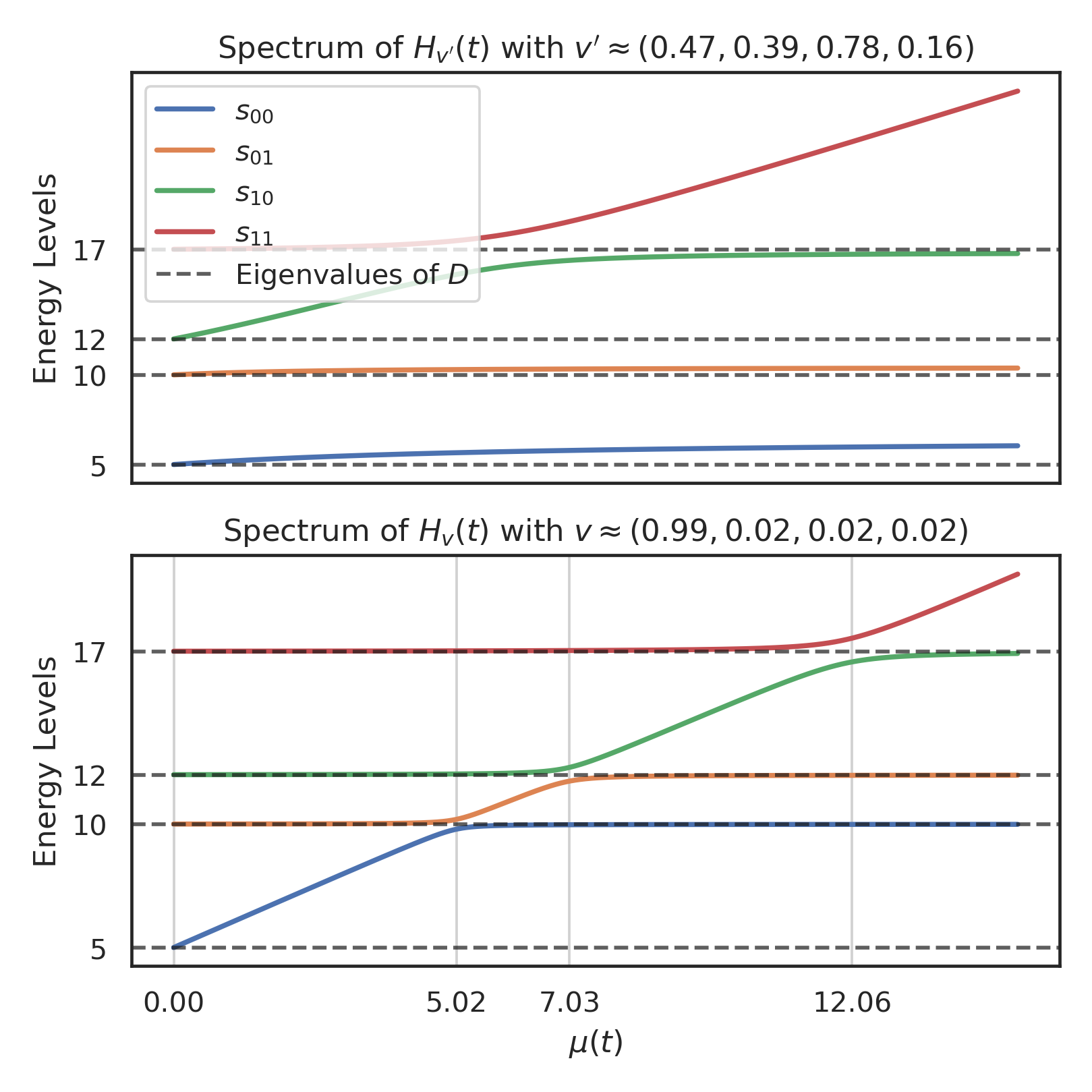
Figure 8:

The systematic progression of eigenvalues associated with $H_{v}(t)$ facilitates an intuitive characterization of the time evolution of the state $\ket{\psi_{\tilde{A}AB}}$ in (67). Let $I\otimes U(t_{f})$ denote the adiabatic evolution operator prescribed by the Hamiltonian $H_{v}(t)$. Then the final evolved state is:

$$\ket{\psi_{\tilde{A}^{\prime}A^{\prime}B^{\prime}}}=\alpha_{00} \ket{\tilde{a}_{0}}U(t_{f})\ket{a_{0}}\ket{b_{0}}$$

$$+\alpha_{11}\ket{\tilde{a}_{1}}U(t_{f})\ket{a_{1}}\ket{b_{0}}$$ (71)

Let us consider the first term $U(t_{f})\ket{a_{0}}\ket{b_{0}}$ of the equation above. Applying Lemma 1 and recalling Theorem 5 we deduce that

$$U(t_{f})\ket{a_{0}}\ket{b_{0}}=\eta_{00}\gamma_{00}(s_{00}I-D)^{-1}\ket{v}$$

$$=\eta_{00}\gamma_{00}\left(\frac{v_{00}}{s_{00}-d_{00}}\ket{a_{0}}\ket{b_{0}}+\frac{\epsilon}{s_{00}-d_{01}}\ket{a_{0}}\ket{b_{1}}\right)+O(\epsilon),$$

where $\eta_{00}$ is a dynamical phase. From the bottom subplot of Figure 8, we see that on the interval $\mathcal{I}_{1}:=(5.02,+\infty)$, the lowest eigenvalue $s_{00}$ converges to the eigenvalue $d_{01}=10$ of $D$. Indeed, by Lemma 9, the coefficient $\epsilon/(s_{00}-d_{01})\approx 1/\epsilon$ is a large number that dominates other coefficients. Hence,

$$U(t_{f})\ket{a_{0}}\ket{b_{0}}\approx\eta_{00}\ket{a_{0}}\ket{b_{1}}.$$ (73)

Let us now examine the evolution of the second term $U(t_{f})\ket{a_{1}}\ket{b_{0}}$ of the equation in (VII.1). Consider the interval $\mathcal{I}_{2}:=(7.03,12.06)$ which can be computed using eigenvalues of $D$ and (25) in Theorem 4. Then for $\mu_{t_{f}}$ in $\mathcal{I}_{2}$, by Lemma 1, we have:

$$U(t_{f})\ket{a_{1}}\ket{b_{0}}=\eta_{10}\gamma_{10}(s_{10}I-D)^{-1}\ket{v}$$ (74)

Since on the interval $\mathcal{I}_{2}$, the eigenvalue $s_{10}$ is not close to any of the eigenvalues and the coefficient $v_{00}\approx 0.9988$ [VII.1] of $\ket{a_{0}}\ket{b_{0}}$ dominates, we have:

$$U(t_{f})\ket{a_{1}}\ket{b_{0}}=\eta_{10}\gamma_{10}(s_{10}I-D)^{-1}\ket{v}$$

$$=\eta_{10}\gamma_{10}\left(\frac{v_{00}}{s_{10}-d_{00}}\ket{a_{0}}\ket{b_{0}}+\sum_{kp\neq 00}\frac{\epsilon}{s_{10}-d_{kp}}\ket{a_{k}}\ket{b_{p}}\right)$$

$$=\eta_{10}\gamma_{10}\frac{v_{00}}{s_{10}-d_{00}}\ket{a_{0}}\ket{b_{0}}+O(\epsilon)$$

Therefore, we have:

$$U(t_{f})\ket{a_{1}}\ket{b_{0}}\approx\eta_{10}\ket{a_{0}}\ket{b_{0}}\approx\eta_{10}\ket{v}$$ (75)

Substituting the results in (73) and (75) into the final state in (VII.1), we get:

$$\ket{\psi_{\tilde{A}^{\prime}A^{\prime}B^{\prime}}}\approx\alpha_{00}\eta_{00}\ket{\tilde{a}_{0}}\ket{a_{0}}\ket{b_{1}}+\alpha_{11}\eta_{10}\ket{\tilde{a}_{1}}\ket{a_{0}}\ket{b_{0}}$$ (76)

We immediately see that $\ket{a_{0}}$ can be factored out. Therefore, the system $A^{\prime}$ is disentangled and pure, whereas system $\tilde{A}^{\prime}$ and $B^{\prime}$ are maximally entangled. Hence, for $\mu_{t_{f}}\in\mathcal{I}_{2}$ and the choice of $\ket{v}$ in (68), we achieved maximum transfer of entanglement.

A similar analysis on the interval $\mathcal{I}_{3}:=(12.06,+\infty)$ which is computed according to (26) in Theorem 4 shows that the entanglement between $\tilde{A}^{\prime}$ and $A^{\prime}$ is reverted back, while $B^{\prime}$ becomes disentangled and pure. To see this, we inspect the bottom subplot of Figure 8 and note that on the interval $\mathcal{I}_{3}$, we have $s_{00}$ and $s_{10}$ being close to $d_{01}=10$ and $d_{11}=17$ respectively. Hence:

$$U(t_{f})\ket{a_{0}}\ket{b_{0}} \approx\eta_{00}\ket{a_{0}}\ket{b_{1}},$$

$$U(t_{f})\ket{a_{1}}\ket{b_{0}} \approx\eta_{10}\ket{a_{1}}\ket{b_{1}}$$ (77)

Therefore, the final state is:

$$\ket{\psi_{\tilde{A}^{\prime}A^{\prime}B^{\prime}}}\approx\alpha_{00}\eta_{00}\ket{\tilde{a}_{0}}\ket{a_{0}}\ket{b_{1}}+\alpha_{11}\eta_{10}\ket{\tilde{a}_{1}}\ket{a_{1}}\ket{b_{1}}$$ (78)

We readily see that $\ket{b_{1}}$ can be factored out, and $\tilde{A}^{\prime}$ and $A^{\prime}$ are maximally entangled. That is, the original entanglement is maximally preserved.

This example illustrates the complex yet ordered nature of adiabatic state evolution and its implications for the entanglement characteristics of a quantum system. From knowledge of the eigenvalues of the matrix $D$, one can compute specific intervals using (31) for the coupling parameter $\mu_{t_{f}}$ where entanglement transfer or preservation occurs.

VIII Non-perturbative Measures of Entanglement and Coherent Information

In this section, we focus on quantifying entanglement transfer or preservation in cases where the interaction term $\outerproduct{v}{v}$ is chosen arbitrarily. As previously discussed in Section VII.1 and illustrated in the top subplot of Figure 8, an arbitrary selection of $\ket{v}$ results in a complex and unordered eigenspectrum dynamics in $H(t)$. As a result, this leads to only partial entanglement transfer or preservation. To accurately assess these effects, we introduce a series of non-perturbative equations. These equations serve as a generalization of the previously presented results.

Our first inquiry centers on quantifying the residual entanglement within $\tilde{A}A$ following its interaction with $B$ during the course of adiabatic evolution, as governed by the Hamiltonian outlined in (16). Our second inquiry focuses on quantifying the entanglement transfer from $A$ to $B$, also following the course of the adiabatic evolution. For the first inquiry, we will work with the direct channel from $A$ to the adiabatically evolved $A^{\prime}$. For the second inquiry, we will work with a complementary channel from $A$ to the adiabatically evolved $B^{\prime}$. We denote the direct and complementary channels as ${A\rightarrow A^{\prime}}$ and ${A\rightarrow B^{\prime}}$, respectively.

A quantum channel’s quantum capacity, i.e., its ability to transmit entanglement, is usually defined through an optimization over the so-called coherent information [11], for parallel uses of the channel with entangled input allowed. The coherent information for the channel ${A\rightarrow A^{\prime}}$, the so-called direct channel, reads:

$$I^{d}=S(A^{\prime})-S\left((\tilde{A}A)^{\prime}\right)$$ (79)

The coherent information for the complementary channel $A\rightarrow B^{\prime}$, reads:

$$I^{c}=S(B^{\prime})-S\left((\tilde{A}B)^{\prime}\right)$$ (80)

Here, $S(\cdot)$ denotes the von Neumann entropy, and its argument denotes a subsystem for which the entropy is computed. Essentially, the coherent information compares joint and marginal von Neumann entropies and finding it positive proves the existence of entanglement. The von Neumann entropy is entanglement monotone if the total system is in a pure state, but its calculation requires the diagonalization of the density operator. This is where the generalization to $\alpha$-Rényi entropy proves useful. Defined for a positive real number $\alpha\neq 1$ as

$$S_{\alpha}(\rho):=\frac{1}{1-\alpha}\log\text{Tr}(\rho^{\alpha}).$$ (81)

The $\alpha$-Rényi entropy encompasses the von Neumann entropy as a special case when $\alpha$ approaches 1. Importantly, the $2$-Rényi entropy $S_{2}(\rho)=-\log\text{Tr}(\rho^{2})$ is directly related to the easy-to-calculate purity $\Tr(\rho^{2})$ of a state.

Recent work has shown that comparing purities of combined and marginal systems tends to be significantly more effective than using von Neumann entropies for witnessing entanglement [12]. Motivated by this insight, we introduce the concept of purity-based coherent information. This alternative formulation for the direct channel $A\rightarrow A^{\prime}$ mirrors the conventional definition as given in (79) and is expressed as:

$$PI^{d}:=P\left((\tilde{A}A)^{\prime}\right)-P\left(A^{\prime}\right)$$ (82)

Similarly, the purity-based coherent information for the complementary channel $A\rightarrow B^{\prime}$ is defined as:

$$PI^{c}=P\left((\tilde{A}B)^{\prime}\right)-P\left(B^{\prime}\right)$$ (83)

Just as coherent information, purity-based coherent information, when positive, indicates the presence of quantum correlations between the subsystems. In contrast to the von Neumann entropy, which requires diagonalization of the density matrix, purities can be computed much more easily, analytically or determined empirically by creating interference between two identical instances of the quantum system [13, 14].

Let us briefly examine a couple of trivial scenarios to illuminate the implications of (82). Assume that after the adiabatic interaction, $(\tilde{A}A)^{\prime}$ is in a pure, maximally entangled state. Under this condition, the subsystem $A^{\prime}$ is maximally mixed. In other words, $P((\tilde{A}A)^{\prime})=1$ and $P(A^{\prime})<1$. This leads to the result that $PI^{d}>0$, affirming the statement that $(\tilde{A}A)^{\prime}$ features entanglement. In a complementary manner, if $PI^{d}>0$ and $(\tilde{A}A)^{\prime}$ is found to be in a pure state, we can once again deduce that $(\tilde{A}A)^{\prime}$ is indeed entangled. Generally, whenever $1\geq P(({A}A)^{\prime})>P(A^{\prime})$ it is always possible to infer that $(\tilde{A}A)^{\prime}$ features entanglement [12].

It is straightforward to transform the equations above into the 2-Rényi-coherent information. First, we take the negative logarithms of $P((\tilde{A}A)^{\prime})$ and $P(A^{\prime})$ in (82). This yields the conditional Rényi entropy $S_{2}(\tilde{A}^{\prime}|A^{\prime})$. Then, we multiply both sides of the equation by the negative one to get to the definition of coherent information. Therefore, the $2$-Rényi-coherent information for the direct channel $A\rightarrow A^{\prime}$ is defined as follows:

$$RI^{d} :=\log P\left((\tilde{A}A)^{\prime}\right)-\log P\left(A^{\prime}\right)$$ (84)

$$=S_{2}(A^{\prime})-S_{2}\left((\tilde{A}A)^{\prime}\right)$$

Similarly, we define the $2$-Rényi-coherent information for the complementary channel $A\rightarrow B^{\prime}$ as:

$$RI^{c} :=\log P\left((\tilde{A}B)^{\prime}\right)-\log P\left(B^{\prime}\right)$$ (85)

$$=S_{2}(B^{\prime})-S_{2}\left((\tilde{A}B)^{\prime}\right)$$

Given the monotonic behaviour of the logarithm function, it can be readily inferred that a positive value for $RI^{d}$ serves as a witness for quantum correlations such as entanglement in $(\tilde{A}A)^{\prime}$. This leads us to establish the following equivalence relation

$$P\left((\tilde{A}A)^{\prime}\right)>P\left(A^{\prime}\right)\iff S_{2}(A^{\prime})>S_{2}\left((\tilde{A}A)^{\prime}\right),$$

or equivalently,

$$RI^{d}>0\iff PI^{d}>0.$$

Similarly, we can show that

$$RI^{c}>0\iff PI^{c}>0.$$ (86)

In light of this equivalence, our subsequent analysis will focus on purities and $PI^{d}$ with $PI^{c}$, which offer the advantage of yielding more straightforward and transparent mathematical expressions. The next section presents the analytical non-perturbative expression for computing (82) and (84).

VIII.1 Coherent information of direct and complementary channels

In this section, we derive analytical expressions for the purity-based coherent information of the direct channel $A\rightarrow A^{\prime}$ and complementary channel $A\rightarrow B^{\prime}$ after the adiabatic interaction of $A$ and $B$, as governed by the Hamiltonian outlined in (16) where the interaction term $\outerproduct{v}{v}$ is arbitrary. Throughout this section, let us assume that the system $\tilde{A}A$ is initialized in a pure entangled state while system $B$ starts as a pure and unentangled state. Under these premises, we derive several theorems and corollaries that characterize the evolution of entanglement from its initial value to arbitrary subsequent values.

We let the system $\tilde{A}A$ start in a pure state and choose an arbitrary basis $\{\ket{\tilde{a}_{k}}\}$ for the Hilbert space $\mathcal{H}_{\tilde{A}}$ of the system $\tilde{A}$. For some fixed $i$ and $j$, we define the state of $\tilde{A}A$ to be

$$\ket{\psi_{\tilde{A}A}}=\alpha_{ii}\ket{\tilde{a}_{i}}\ket{a_{i}}+\alpha_{jj}\ket{\tilde{a}_{j}}\ket{a_{j}},$$ (87)

where $\alpha_{ii}$ and $\alpha_{jj}$ are complex coefficients. We may assume that $|\alpha_{ii}|^{2}=|\alpha_{jj}|^{2}$, or in other words, the initial state $\ket{\psi_{\tilde{A}A}}$ starts out entangled. Then the joint initial state of $\tilde{A}AB$ is:

$$\ket{\psi_{\tilde{A}AB}}=\alpha_{ii}\ket{\tilde{a}_{i}}\ket{a_{i}}\ket{b_{0}}+\alpha_{jj}\ket{\tilde{a}_{j}}\ket{a_{j}}\ket{b_{0}}$$ (88)

Since $\ket{a_{i}}$ and $\ket{b_{0}}$ are eigenstates of the initial Hamiltonian $D$, by Lemma 1, the adiabatically evolved state is

$$\ket{\psi_{\tilde{A}^{\prime}A^{\prime}B^{\prime}}} =\alpha_{ii}\ket{\tilde{a}_{i}}U(t_{f})(\ket{a_{i}}\ket{b_{0}})$$

$$\hbox{}\quad\quad\quad+\alpha_{jj}\ket{\tilde{a}_{j}}U(t_{f})(\ket{a_{j}}\ket{b_{0}})$$ (89)

$$=\alpha_{ii}\eta_{i0}\ket{\tilde{a}_{i}}\ket{s_{i0}}+\alpha_{jj}\eta_{j0}\ket{\tilde{a}_{j}}\ket{s_{j0}},$$ (90)

where $\eta_{i0}$ and $\eta_{j0}$ are dynamical phases. We show that the purity-based coherent information of the direct channel $A\rightarrow A^{\prime}$ can be computed as follows.

Theorem 10.

Consider a tripartite quantum system $\tilde{A}AB$ initially prepared in a state described by (88). Assume that the system undergoes adiabatic evolution according to the Hamiltonian $H(t)$, as defined by (16) with $\outerproduct{v}{v}$ being arbitrary. Then the purity-based coherent information for the direct channel $A\rightarrow A^{\prime}$ is given by

$$PI^{d} =\nu\Tr[\Tr_{B}[\outerproduct{s_{i0}}{s_{j0}}]\Tr_{B}[\outerproduct{s_{j0}}{s_{i0}}]\Big{]}$$ (91)

$$-\nu\Tr[\Tr_{B}[\outerproduct{s_{i0}}{s_{i0}}]\Tr_{B}[\outerproduct{s_{j0}}{s_{j0}}]\Big{]},$$

where $\nu=2|\alpha_{ii}|^{2}|\alpha_{jj}|^{2}$.

Similarly, the purity-based coherent information of the complementary channel $A\rightarrow B^{\prime}$ is given by the following theorem.

Theorem 11.

Under the assumptions stated in Theorem 10, the purity-based coherent information for the complementary channel $A\rightarrow B^{\prime}$ is given by

$$PI^{c} =\nu\Tr[\Tr_{A}[\outerproduct{s_{i0}}{s_{j0}}]\Tr_{A}[\outerproduct{s_{j0}}{s_{i0}}]\Big{]}$$

$$-\nu\Tr[\Tr_{A}[\outerproduct{s_{i0}}{s_{i0}}]\Tr_{A}[\outerproduct{s_{j0}}{s_{j0}}]\Big{]},$$ (92)

where $\nu=2|\alpha_{ii}|^{2}|\alpha_{jj}|^{2}$.

We conclude this section by presenting two important lemmas that are used to derive explicit formulas for the aforementioned coherent information measures in Theorem 10 and Theorem 11. Given the relation in Lemma 1, we have:

$$\ket{s}=\gamma(sI-D)^{-1}\ket{v}$$ (93)

Then, we can explicitly compute the purity of the reduced density matrix of $\outerproduct{s}{s}$.

Lemma 12.

Let $\rho_{AB}:=\outerproduct{s}{s}$ and $\rho_{A}:=\Tr_{B}\left[\rho_{AB}\right]$, then the purity of $\rho_{A}$ is given by

$$P(\rho_{A})=\gamma^{4}\sum_{ijkp}\frac{v_{ij}}{(s-d_{ij})}\frac{v^{*}_{kj}}{(s-d_{kj})}\frac{v_{kp}}{(s-d_{kp})}\frac{v^{*}_{ip}}{(s-d_{ip})},$$ (94)

where $v_{ij}=\bra{v}\ket{a_{i},b_{j}}$ is a coefficient matrix of $\ket{v}$ in the eigenbasis $\{\ket{a_{i}}\ket{b_{j}}\}_{ij}$ of $D$ and

$$\gamma=\left(\sum_{ij}\left|\frac{v_{ij}}{s-d_{ij}}\right|^{2}\right)^{-1/2}.$$ (95)

We have presented a non-perturbative, explicit formula for calculating the purity of a reduced density matrix corresponding to the eigenstates of the final Hamiltonian $H(t_{f})$. Below, we introduce a lemma, which is a generalization of Lemma 12. This lemma is instrumental in deriving explicit equations in Theorem 10 and Theorem 11.

Lemma 13.

Let $\ket{s}$, $\ket{s^{\prime}}$, $\ket{s^{\prime\prime}}$ and $\ket{s^{\prime\prime\prime}}$ be eigenstates defined as in (93). Then the following holds:

$$\Tr[\Tr_{B}[\outerproduct{s}{s^{\prime}}]\Tr_{B}[\outerproduct{s^{\prime\prime}}{s^{\prime\prime\prime}}]\Big{]}=\\ \gamma\gamma^{\prime}\gamma^{\prime\prime}\gamma^{\prime\prime\prime}\sum_{ijkp}\frac{v_{ij}}{(s-d_{ij})}\frac{v^{*}_{kj}}{(s^{\prime}-d_{kj})}\frac{v_{kp}}{(s^{\prime\prime}-d_{kp})}\frac{v^{*}_{ip}}{(s^{\prime\prime\prime}-d_{ip})}$$ (96)

Therefore, whenever $s=s^{\prime},s^{\prime\prime},s^{\prime\prime\prime}$, the equation in (96) becomes $P(\rho_{A})$ in (94). Now, using Lemma 12 or Lemma 13 it is straightforward to derive explicit equations for computing the quantities $\Tr[\Tr_{B}[\outerproduct{s_{i0}}{s_{j0}}]]$ and $\Tr[\Tr_{B}[\outerproduct{s_{i0}}{s_{i0}}]]$ that appear in Theorem 10 and Theorem 11. This, in turn, yields explicit non-perturbative equations for purity-based coherent information $PI^{d}$ and $PI^{c}$.

VIII.2 Maximum and minimum of coherent information

In this section, we show that the construction of $\ket{v}$ in Theorem 4 that accomplishes entanglement transfer or preservation is just a special case of Theorem 10 and Theorem 11 that maximizes/minimizes $PI^{d}$ and $PI^{c}$.

We commence by examining the initial quantum state specified by equation (88), with the coefficients $\alpha_{ii}$ and $\alpha_{jj}$ each set to $1/\sqrt{2}$. A straightforward analysis reveals that initially (at $\mu=0$), the coherent information of the direct quantum channel from $A$ to itself stands at the maximum $PI_{\text{init}}^{d}=1/2$. Concurrently, the initial coherent information associated with the complementary channel from $A$ to $B$ is at its minimum $PI_{\text{init}}^{c}=-1/2$. Given that $PI_{\text{init}}^{d}$ is positive, it is inferred that the system $\tilde{A}A$ is entangled, a fact that is directly observable from the initial state configuration. The derivation that $PI_{\text{init}}^{d}=1/2$ is achieved through the application of Theorem 10, under the assumption that the system has not undergone evolution, resulting in $\ket{s_{i0}}=\ket{a_{i}}\ket{b_{0}}$ and $\ket{s_{j0}}=\ket{a_{j}}\ket{b_{0}}$. Therefore, the calculation proceeds as follows:

$$PI_{\text{init}}^{d} =\nu\Tr[\Tr_{B}[\ket{a_{i}}\ket{b_{0}}\bra{a_{j}}\bra{b_{0}}]\Tr_{B}[\ket{a_{j}}\ket{b_{0}}\bra{a_{i}}\bra{b_{0}}]\Big{]}$$

$$-\nu\Tr[\Tr_{B}[\ket{a_{i}}\ket{b_{0}}\bra{a_{i}}\bra{b_{0}}]\Tr_{B}[\ket{a_{j}}\ket{b_{0}}\bra{a_{j}}\bra{b_{0}}]\Big{]}$$

$$=\nu\Tr[\outerproduct{a_{i}}{a_{j}}\outerproduct{a_{j}}{a_{i}}]-\nu\Tr[\outerproduct{a_{i}}{a_{i}}\outerproduct{a_{j}}{a_{j}}]$$

$$=\nu\Tr[\outerproduct{a_{i}}{a_{i}}]$$

$$=2|\alpha_{ii}|^{2}|\alpha_{jj}|^{2}$$

$$=\frac{2}{4}=\frac{1}{2}$$

The subsequent application of Theorem 11 (where we trace over $A$) yields $PI_{\text{init}}^{c}=-1/2$.

We now introduce an interaction term $\mu(t)\outerproduct{v}{v}$ to adiabatically evolve the initial state, where $\ket{v}$ is constructed as specified in Theorem 4, and $\mu(t_{f})$ is selected based on the interval defined in equation (25). Specifically, the dominant component of $\ket{v}$, $v_{i0}$, is set to $1-(nm-1)\epsilon^{2}$, and $\mu(t_{f})$ is chosen from the interval $((d_{j0}-d_{i0})/|v_{i0}|^{2},(d_{j1}-d_{i0})/|v_{i0}|^{2})$.

By employing Theorem 5 and Theorem 11, we demonstrate that the coherent information of the complementary channel from $A$ to $B^{\prime}$, denoted as $PI_{\text{final}}^{c}$, tends to its maximum value $1/2$ as $\epsilon$ tends to zero. This signifies that the entanglement initially present between $A$ and $\tilde{A}$ has been almost completely transferred to $B$ over the course of adiabatic evolution. The calculation for the coherent information of the complementary channel from $A$ to $B^{\prime}$ is as follows:

$$PI_{\text{final}}^{c} =\nu\Tr[\Tr_{A}[\outerproduct{s_{i0}}{s_{j0}}]\Tr_{A}[\outerproduct{s_{j0}}{s_{i0}}]\Big{]}$$

$$-\nu\Tr[\Tr_{A}[\outerproduct{s_{i0}}{s_{i0}}]\Tr_{A}[\outerproduct{s_{j0}}{s_{j0}}]\Big{]}$$ (97)

Due to the construction of $\ket{v}$ and the choice of $\mu(t_{f})$, by Theorem 5 we know that as $\epsilon\rightarrow 0$, we have:

$$\ket{s_{i0}} =U(t_{f})\ket{a_{i}}\ket{b_{0}}\rightarrow\ket{a_{i}}\ket{b_{1}},$$

$$\ket{s_{j0}} =U(t_{f})\ket{a_{j}}\ket{b_{0}}\rightarrow\ket{a_{i}}\ket{b_{0}}$$

Therefore, in the limit of $\epsilon\rightarrow 0$, we get:

$$PI_{\text{final}}^{c} =\nu\Tr[\Tr_{A}[\ket{a_{i}}\ket{b_{1}}\bra{a_{i}}\bra{b_{0}}]\Tr_{A}[\ket{a_{i}}\ket{b_{0}}\bra{a_{i}}\bra{b_{1}}]$$

$$-\nu\Tr[\Tr_{A}[\ket{a_{i}}\ket{b_{1}}\bra{a_{i}}\bra{b_{1}}]\Tr_{A}[\ket{a_{i}}\ket{b_{0}}\bra{a_{i}}\bra{b_{0}}]\Big{]}$$

$$=\nu\Tr[\outerproduct{b_{1}}{b_{0}}\outerproduct{b_{0}}{b_{1}}]-\nu\Tr[\outerproduct{b_{1}}{b_{1}}\outerproduct{b_{0}}{b_{0}}]$$

$$=\nu\Tr[\outerproduct{b_{1}}{b_{1}}]$$

$$=2|\alpha_{ii}|^{2}|\alpha_{jj}|^{2}$$

$$=\frac{2}{4}=\frac{1}{2}$$

Correspondingly, it can be shown that in the limit $\epsilon\rightarrow 0$, we get $PI_{\text{final}}^{d}=-1/2$.

Hence, we establish that the value of coherent information of the complementary channel $PI_{\text{final}}^{c}$ at the end of the adiabatic evolution matches the initial maximum value of coherent information of the direct channel $PI_{\text{init}}^{d}$ of the system prior to evolution, confirming the nearly complete transfer of entanglement from $A$ to $B$ during the process.

IX Outlook

Entanglement, as a phenomenon without classical analog, is not only of foundational interest but also of practical importance as a key resource in quantum technologies. We developed here new nonperturbative methods to analyze the creation and transmission of entanglement which, therefore, possess potential for wide applicability. Below, we outline a few directions for further research and applications.

Tracing entanglement creation and transfer to swaps of eigenstates at avoided level crossings. We decomposed adiabatic interactions into a sequence of projector activations. For each of these activations, we then traced the changes of entanglement to a sequence of eigenstate swaps that occur at avoided level crossings. The dynamics of the entanglement, i.e., the speed of the underlying swaps of eigenstates, depends on how narrow the level crossings are avoided, and this can be traced back to how closely the currently activated projector $|v\rangle\langle v|$ is aligned to any prior eigenvector, $|d_{k}\rangle$. We showed this explicitly for bi-partite and tri-partite systems, but it should be straightforward to extend this analysis to the dynamics of the more complex types of entanglement that can arise in $n$-partite systems for $n>3$.

New entanglement measures. Based on our finding that the dynamics of entanglement can be traced back to eigenstate swaps at avoided level crossings, the development of new measures of multi-partite entanglement may be possible. For example, it will be interesting to explore measures based on the minimum number of projector activations, avoided level crossings and associated state swaps that are needed to create a given entangled state from an unentangled state. Such measures are nontrivial since, for example, for a projector activation to arrive at a desired critical $\mu$ value, it may first have to pass through other critical $\mu$ values that could impart collateral damage to the effort of generating the entangled target state. Similar to Rubik’s cube, a group theoretic analysis could be developed here, or at least mnemonic devices. Inspired by the categorical approach to knot invariants [15, 16], it may also be possible to use category-theoretic methods to develop entanglement measures or entanglement invariants (i.e., functors) based on our findings. To this end, the over and under crossings in knots would be replaced by the different but reminiscent structure of eigenvector swaps at avoided level crossings. While the Reidemeister moves of knots lead to the quantum Yang Baxter equation whose solutions provide knot invariant polynomials, as is well known [17], here it will be very interesting to pursue an analog approach by exploring possible analogs of Reidemeister moves for avoided level crossings.

Quantitative tracking of entanglement with coherent information. In order to quantitatively track the creation and transfer of entanglement during interactions, we calculated coherent informations based on the 2-Renyi entropy. This allowed us to use our nonpertubative approach to track the dynamics of entanglement during the full duration of even strong interactions. For prior results on the perturbative tracking of the dynamics of entropies and entanglement during interactions, see,[18, 19, 20]. It will also be interesting to apply our nonperturbative methods to the $1$-Renyi entropy-based coherent information since this will provide lower bounds to the quantum channel capacities of the direct and complementary channels.

Connecting computational complexity and usage of the resource of entanglement. Our results quantitatively relate a mathematical problem’s computational complexity, as measured by the maximum speed of its adiabatic quantum computability, to the adiabatic quantum computation’s usage of the resource of entanglement. Concretely, we found quantitative relationships between the efficiency of the adiabatic generation and/or transfer of entanglement during an avoided level crossing on one hand, and how narrowly the level crossing is avoided on the other hand. These results link, therefore, the adiabatic dynamics of entanglement to energy gaps and, therefore, to the slowdown required to keep the quantum computation adiabatic.

Also in quantum annealing, which has already found industrial applications [21, 22, 23, 24, 25], it should be very interesting to explore analogously the relationship between computational complexity, in the sense of the maximum speed of the computation, and the usage of the resource of entanglement.

Non-adiabatic quantum computation and Landau-Zener. More generally, the role of entanglement in adiabatic and adiabatic-inspired algorithms is an active area of research [26, 27, 28, 29, 30, 31, 32, 33] for which our results could provide new tools. For example, the group theoretic approach in Section VI could enable qualitative tracking of entanglement, also possibly using graphical strategies, [34, 35], without the need for full numerical simulations.

In particular, it will be interesting to explore how the relationship between computational speed and the usage of the resource of entanglement that we found here generalizes to adiabatic-inspired and diabatic quantum computing algorithms such as QAOA [26] and adiabatic/diabatic quantum algorithms, see, e.g., [36, 28], as well as to counter-diabatic algorithms, see, e.g., [37, 38]. To this end, it will be straightforward, for example, to generalize our present results by strategically permitting diabatic state transitions, namely by using the Landau-Zener transition probabilities to allow controlled non-adiabaticity at chosen avoided level crossings.

Quantum Error Correction. In quantum processors, an important source of quantum errors is the inadvertent creation or transfer of entanglement due to unintended interactions among qubits or between qubits and their environment. Quantum error correction aims to protect quantum information through encoding and decoding techniques. Numerous studies, including those in adiabatic quantum computation, have focused on this goal [39, 40, 41, 42, 43].

In this context, the theory presented in this work demonstrates, for example, that if a qubit $A$ is entangled with an ancilla $\tilde{A}$, it is possible to surgically disentangle $A$ from $\tilde{A}$ by having a qubit $B$ interact with $A$ using for example a tailored edge-case-like Hamiltonian. Equally, it is possible to choose the interaction between $B$ and $A$ such that the entanglement with $\tilde{A}$ becomes distributed between $A$ and $B$, see e.g., the tri-partite entangled state (5). This ability to surgically entangle, disentangle and transfer entanglement, Hilbert space dimension by Hilbert space dimension, i.e., on the most elementary level, should be useful for quantum error prevention and correction in adiabatic, adiabatic-inspired and algorithmic quantum computation, see, e.g., [39, 40, 41, 42, 43]. To this end, it should be very interesting to explore training machine learning models to use these surgical tools for quantum error prevention and correction adapted to the hardware at hand. For examples of machine learning applied to quantum computation (including adiabatic computation) and error correction, see e.g., [44, 45, 46, 47, 48, 49, 50, 51, 52].

Acknowledgements
AK and EG acknowledge support through a grant from the National Research Council of Canada (NRC). AK also acknowledges a Discovery Grant from the National Science and Engineering Council of Canada (NSERC), a Discovery Project grant of the Australian Research Council (ARC). EG acknowledges partial support through Mitacs Accelerate Fellowship. EG also acknowledges the support provided by NSERC through a Canada Graduate Scholarship – Doctoral Program (CGS-D).

Appendix A Proof of Lemma 1

Our goal is to derive an explicit expression for the eigenstate $\ket{s}$ of $H(t)$. Let $s:=s(\mu(t))$ and $\mu:=\mu(t)$. We want to consider the following eigenvector equation:

$$H(t)\ket{s} =s\ket{s}$$ (98)

$$\left(D+\mu\outerproduct{v}{v}\right)\ket{s} =s\ket{s}$$ (99)

Rearranging terms, we get:

$$(sI-D)\ket{s} =\mu\ket{v}\innerproduct{v}{s}$$ (100)

$$\ket{s} =\mu\innerproduct{v}{s}(sI-D)^{-1}\ket{v}$$ (101)

Finally, we set $\gamma=1/\|(sI-D)^{-1}\ket{v}\|$ and redefine $\ket{s}$ as

$$\ket{s}:=\gamma(sI-D)^{-1}\ket{v}.$$ (102)

Appendix B Proof of Lemma 2

The statements of Lemma 2 is simply applying the adiabatic theorem in [3] to the result of Lemma 1.

Appendix C Proof of Lemma 3

Consider an $N\times N$ Hermitian matrix $H(s)=D+\mu(s)\outerproduct{v}{v}$, where $\mu(s)$ is a scalar function to be determined. Let $\{d_{k}\}$ and $\{\ket{d_{k}}\}$ be the eigenvalues and eigenvectors of $D$. Define $v_{k}=\innerproduct{d_{k}}{v}$. For a real number $s$, the characteristic polynomial $p(s)$ of $H(s)$ can be expressed as:

$$p(s) =\det\left(H(s)-sI\right)$$

$$=\det\left(D+\mu(s)\outerproduct{v}{v}-sI\right)$$ (103)

Using Cauchy’s formula for the determinant of a rank-one perturbation [53, Section 0.8], we have:

$$p(s)=\det(D-sI)\left(1-\mu(s)\sum_{k=0}^{N-1}\frac{|v_{k}|^{2}}{s-d_{k}}\right)$$ (104)

Define $\mu(s)$ as:

$$\mu(s)=\left(\sum_{k=0}^{N-1}\frac{|v_{k}|^{2}}{s-d_{k}}\right)^{-1}$$ (105)

This choice of $\mu(s)$ ensures that the factor within the parentheses in the determinant expression [104] becomes zero, leading to $p(s)=0$. Therefore, $s$ is an eigenvalue of $H(s)$.

Appendix D Proof of Theorem 4

The proof is the direct application of Theorem 5 or Theorem 6. Let the system $\tilde{A}A$ be entangled and $B$ be in a pure and unentangled state:

$$\ket{\psi_{\tilde{A}AB}}=\alpha_{ii}\ket{\tilde{a}_{i}}\ket{a_{i}}\ket{b_{0}}+\alpha_{jj}\ket{\tilde{a}_{j}}\ket{a_{j}}\ket{b_{0}}.$$ (106)

For $\epsilon>0$ and fixed index $i$, define $\ket{v}$ in the eigenbasis $\{\ket{a_{k}}\ket{b_{p}}\}_{kp}$ of $H_{A}$ and $H_{B}$ such that

$$v_{kp}=\begin{cases}1-(nm-1)\epsilon^{2}&\text{for }k=i,p=0,\\ \epsilon&\text{otherwise}.\end{cases}$$ (107)

Suppose that $\mu_{t_{f}}$ is in the interval $\left(\frac{d_{j0}-d_{i0}}{|v_{i0}|^{2}},\frac{d_{j1}-d_{i0}}{|v_{i0}|^{2}}\right)$. Then, by Theorem 5, at the limit $\epsilon\rightarrow 0$, the state $\ket{a_{i}}\ket{b_{0}}$ evolves into the next higher-energy state $\ket{a_{i}}\ket{b_{1}}$, while the state $\ket{a_{j}}\ket{b_{0}}$ evolves into $\ket{a_{i}}\ket{b_{0}}$. Hence, the final state is:

$$\ket{\psi_{\tilde{A}^{\prime}A^{\prime}B^{\prime}}} =\eta_{ii}\alpha_{ii}\ket{\tilde{a}_{i}}\ket{a_{i}}\ket{b_{1}}+\eta_{jj}\alpha_{jj}\ket{\tilde{a}_{j}}\ket{a_{i}}\ket{b_{0}}$$

$$=\ket{a_{i}}\otimes\left(\eta_{ii}\alpha_{ii}\ket{\tilde{a}_{i}}\ket{b_{1}}+\eta_{jj}\alpha_{jj}\ket{\tilde{a}_{j}}\ket{b_{0}}\right)$$ (108)

In the above, $\eta_{ii}$ and $\eta_{jj}$ are dynamical phases that were acquired during the evolution. Importantly, we immediately see that $\ket{a_{i}}$ can be factored out, which implies that system $A$ is now untangled and pure, whereas $\tilde{A}$ and $B$ are entangled.

Suppose that $\mu_{t_{f}}>\frac{d_{j1}-d_{i0}}{|v_{i0}|^{2}}$. Then, by Theorem 5, at $\epsilon\rightarrow 0$, the states $\ket{a_{i}}\ket{b_{0}}$ and $\ket{a_{j}}\ket{b_{0}}$ evolve to their next respective higher-energy states: $\ket{a_{i}}\ket{b_{1}}$ and $\ket{a_{j}}\ket{b_{1}}$. Hence, the final state of the total system is:

$$\ket{\psi_{\tilde{A}AB}}=\eta^{\prime}_{ii}\alpha_{ii}\ket{\tilde{a}_{i}}\ket{a_{i}}\ket{b_{1}}+\eta^{\prime}_{jj}\alpha_{jj}\ket{\tilde{a}_{j}}\ket{a_{j}}\ket{b_{1}}$$ (109)

In the above, $\eta^{\prime}_{ii},\eta^{\prime}_{jj}$ are dynamical phases acquired during the evolution. Furthermore, the state $\ket{b_{1}}$ can be factored out. We deduce that the system $B$ is now pure and unentangled, whereas $\tilde{A}$ and $A$ are entangled as in the initial state. As such, the entanglement structure is preserved.

Appendix E Proof of Lemma 9

We first prove the Lemma 9 and use it to prove Theorem 5. Let $N$ be the dimension of the Hilbert space $H(t)$ acts on. Let $\{\ket{d_{j}}\}_{j=0}^{N-1}$ be the eigenbasis of $D$ with eigenvalues $d_{0}<\cdots<d_{N-1}$. Consider the characteristic polynomial of $H(t)$ in the eigenbasis $D$ and $\mu\geq 0$:

$$p(s) =\det(D+\mu\outerproduct{v}{v}-sI)$$ (110)

$$=\det(D-sI)\left(1+\mu\sum_{j=0}^{N-1}\frac{|v_{j}|^{2}}{d_{j}-s}\right)$$ (111)

$$=\prod_{j=0}^{N-1}(d_{j}-s)\left(1+\mu\sum_{j=0}^{N-1}\frac{|v_{j}|^{2}}{d_{j}-s}\right).$$ (112)

Fix index $i$ and construct $\ket{v}$ according to (28) in Theorem 5. Then,

$$v_{j}=\begin{cases}1-(N-1)\epsilon^{2}&\text{ for }j=i,\\ \epsilon&\text{ otherwise.}\end{cases}$$ (113)

Without loss of generality, assume that $i=0$, then $v_{0}=1-(N-1)\epsilon^{2}$ and $v_{j}=\epsilon$ for $j>0$. The characteristic polynomial becomes:

$$p(s)=\prod_{j=0}^{N-1}(d_{j}-s)\left(1+\mu\frac{|v_{0}|^{2}}{d_{0}-s}+\mu\epsilon^{2}\sum_{j=1}^{N-1}\frac{1}{d_{j}-s}\right)$$ (114)

For any index $p$, due to the interlacing inequality, there exists eigenvalue $s$ of $H(t)$ such that $d_{p}\leq s<d_{p+1}$. Without loss of generality and for simplicity, we consider $p=0$. Then, $d_{0}\leq s<d_{1}$ for $\mu\geq 0$. Hence, we have:

$$p(s)=\prod_{j=0}^{N-1}(d_{j}-s)\left(1+\mu\frac{|v_{0}|^{2}}{d_{0}-s}+\mu\epsilon^{2}\sum_{j=1}^{N-1}\frac{1}{d_{j}-s}\right)=0$$ (115)

Assuming $\mu>0$, we get $d_{0}<s<d_{1}$. Therefore, we must have

$$1+\mu\frac{|v_{0}|^{2}}{d_{0}-s}+\mu\epsilon^{2}\sum_{j=1}^{N-1}\frac{1}{d_{j}-s}=0.$$ (116)

Rewrite the above as

$$1+\mu\frac{|v_{0}|^{2}}{d_{0}-s}+\mu\epsilon^{2}\frac{1}{d_{1}-s}+\mu\epsilon^{2}\sum_{j=2}^{N-1}\frac{1}{d_{j}-s}=0.$$ (117)

Since $d_{0}<s<d_{1}<\cdots<d_{N-1}$, we have $d_{j}-s>d_{j}-d_{1}$ for $j\geq 2$. It follows that

$$\sum_{j=2}^{N-1}\frac{1}{d_{j}-s}<\sum_{j=2}^{N-1}\frac{1}{d_{j}-d_{1}}.$$ (118)

Define $Z:=\sum_{j=2}^{N-1}\frac{1}{d_{j}-d_{1}}$ and note that it is independent of $s$ and hence independent of $\mu$. Thus,

$$1+\mu\frac{|v_{0}|^{2}}{d_{0}-s}+\mu\epsilon^{2}\frac{1}{d_{1}-s}+\mu\epsilon^{2}Z>0.$$ (119)

Rearranging yields:

$$\epsilon^{2}\frac{1}{d_{1}-s}>-\frac{1}{\mu}+\frac{|v_{0}|^{2}}{s-d_{0}}-\epsilon^{2}Z.$$ (120)

Since $d_{0}<s<d_{1}$, we have $s-d_{0}<d_{1}-d_{0}$. Therefore, $|v_{0}|^{2}/(s-d_{0})>|v_{0}|^{2}/(d_{1}-d_{0})$. Using this, we get

$$\epsilon^{2}\frac{1}{d_{1}-s}>-\frac{1}{\mu}+\frac{|v_{0}|^{2}}{d_{1}-d_{0}}-\epsilon^{2}Z.$$ (121)

Rearranging terms yields:

$$\epsilon^{2}+\epsilon^{2}(d_{1}-s)Z>(d_{1}-s)\left(-\frac{1}{\mu}+\frac{|v_{0}|^{2}}{d_{1}-d_{0}}\right)$$ (122)

Since $d_{1}-s<d_{1}-d_{0}$, we can write:

$$\epsilon^{2}+\epsilon^{2}(d_{1}-d_{0})Z>(d_{1}-s)\left(-\frac{1}{\mu}+\frac{|v_{0}|^{2}}{d_{1}-d_{0}}\right)$$ (123)

The above can be rewritten as:

$$\frac{\epsilon^{2}(1+(d_{1}-d_{0})Z)}{-\frac{1}{\mu}+\frac{|v_{0}|^{2}}{d_{1}-d_{0}}}>d_{1}-s$$ (124)

Note that the denominator can be re-expressed as:

$$-\frac{1}{\mu}+\frac{|v_{0}|^{2}}{d_{1}-d_{0}}=\frac{|v_{0}|^{2}\mu+d_{0}-d_{1}}{(d_{1}-d_{0})\mu}$$ (125)

Hence, (124) can be written as:

$$\frac{\epsilon^{2}(1+(d_{1}-d_{0})Z)(d_{1}-d_{0})\mu}{|v_{0}|^{2}\mu+d_{0}-d_{1}}>d_{1}-s$$ (126)

Since $\mu>(d_{1}-d_{0})/|v_{0}|^{2}$, we have $|v_{0}|^{2}\mu+d_{0}-d_{1}>0$. Finally, we note that $|v_{0}|^{2}<1$, therefore $|v_{0}|^{2}\mu<\mu<2\mu$. Thus, we have:

$$\frac{\epsilon^{2}(1+(d_{1}-d_{0})Z)(d_{1}-d_{0})2\mu}{\mu+d_{0}-d_{1}}>d_{1}-s$$ (127)

We can eliminate the dependence on $\mu$ by letting $\mu\rightarrow+\infty$. In the limit $\mu\rightarrow+\infty$, we get a tighter bound:

$$\epsilon^{2}\left(1+(d_{1}-d_{0})Z\right)(d_{1}-d_{0})2>d_{1}-s$$ (128)

Using similar arguments as above, it is straightforward to show that for $0<\mu<d_{1}-d_{0}<(d_{1}-d_{0})/|v_{0}|^{2}$ and $d_{1}<s<d_{2}$, we have

$$\frac{\epsilon^{2}\mu(d_{1}-d_{0})}{d_{1}-\mu-d_{0}}\geq s-d_{1}.$$ (129)

We note that the bound can be saturated for $\mu=0$. In this case, we have $H(t)=D$, which means $s=d_{1}$. This proves Lemma 9.

Appendix F Proof of Theorem 5

We now prove Theorem 5. By Lemma 1 and Lemma 2, we have

$$U(t_{f})\ket{d_{k}}=\gamma(sI-D)^{-1}\ket{v},$$ (130)

where eigenvalue $d_{k}<s<d_{k+1}$. For $0<\mu<(d_{k}-d_{i})/|v_{i}|^{2}$, by Lemma 9, we get that there exists $C_{2}\geq 0$ such that

$$s-d_{k}\leq C_{2}\epsilon^{2}.$$ (131)

Furthermore, we have:

$$\frac{\epsilon}{s-d_{k}}\geq\frac{\epsilon}{C_{2}\epsilon^{2}}=\frac{1}{C_{2}\epsilon}$$ (132)

It follows that the component $\innerproduct{s}{d_{k}}$ of $\ket{s}$ tends to dominate all other components:

$$\innerproduct{s}{d_{k}}=\gamma\frac{v_{k}}{s-d_{k}}=\gamma\frac{\epsilon}{s-d_{k}}\rightarrow 1\text{ as }\epsilon\rightarrow 0$$ (133)

We remark that the normalization constant $\gamma$ prevents the equation above blow up by trending toward zero together with $\epsilon$. Therefore, $\ket{s}\rightarrow\ket{d_{k}}$ as $\epsilon\rightarrow 0$. This proves (30).

Now, suppose that $(d_{k+1}-d_{i})/|v_{i}|^{2}<\mu$ and as before $d_{k}<s<d_{k+1}$. Then by Lemma 9, there exists $C_{1}$ such that:

$$d_{k+1}-s<C_{1}\epsilon^{2}$$ (134)

It follows that

$$\innerproduct{s}{d_{k+1}}=\gamma\frac{v_{k+1}}{s-d_{k+1}}=\gamma\frac{\epsilon}{s-d_{k+1}}<-\gamma\frac{1}{C_{1}\epsilon}.$$ (135)

Hence, the component $\innerproduct{s}{d_{k+1}}$ of $\ket{s}$ approaches $-1$ as $\epsilon$ tends to zero. Also, as $\epsilon$ tends to zero, so does $\gamma$. This proves (34).

For a fixed $\mu\in\left(\frac{d_{k}-d_{i}}{|v_{i}|^{2}},\frac{d_{k+1}-d_{i}}{|v_{i}|^{2}}\right)$, we have $d_{k}<s<d_{k+1}$. Therefore, the component

$$\innerproduct{s}{d_{i}}=\gamma\frac{v_{i}}{s-d_{i}}=\gamma\frac{1-(N-1)\epsilon^{2}}{s-d_{i}}$$ (136)

must converge to $1$ as $\epsilon$ tends to zero and $\gamma$ tends to $s-d_{i}$. This proves (32).

Appendix G Proof of Theorem 6

Theorem 6 is a restatement of Theorem 5 with a focus on the critical points $\mu_{k+1}:=(d_{k+1}-d_{k})/|v_{i}|^{2}$ instead of the intervals given in Theorem 5. We only note that $\mu(t)$ is a monotonous function of time and hence is invertible. Therefore, for $\mu(t)=\mu_{k+1}\pm\Delta\mu$, we can solve for $t$ to get the critical time point $t(\mu_{k+1}\pm\Delta\mu)$ around which the eigenstate transitions are happening.

Appendix H Proof of Theorem 8

For an index $k$, define $s_{k}:=s_{k}(\mu)$. Recall that for $\mu\geq 0$, $s_{k}\leq d_{k+1}\leq s_{k+1}$. We will show that for the construction of $\ket{v}$ as in Theorem 5 there exists $C_{0}>0$ such that

$$d_{k+1}-s_{k} >C_{0}\epsilon^{2},$$ (137)

$$s_{k+1}-d_{k+1} \geq 0.$$ (138)

Therefore, $d_{k+1}-s_{k}+s_{k+1}-d_{k+1}=s_{k+1}-s_{k}>C_{0}\epsilon^{2}$.

For the case $\mu<0$, we will simply have a vertically mirrored behaviour. That is

$$s_{k-1}\leq d_{k-1}\leq s_{k}\leq d_{k},$$ (139)

and it will follow that

$$s_{k}-d_{k-1} >C_{0}\epsilon^{2},$$ (140)

$$d_{k-1}-s_{k-1} >0.$$ (141)

Hence, $s_{k}-s_{k-1}>C_{0}\epsilon^{2}$.

Since the case $\mu<0$ is the mirrored version of the case $\mu\geq 0$, we prove the case for the positive $\mu$ for which $s_{k}\leq d_{k+1}\leq s_{k+1}$.

Without loss of generality, fix $i=0$, then $v_{0}=1-(N-1)\epsilon^{2}$ and $v_{j}=\epsilon$ for $j>0$. Also, for notation clarity, fix $k=0$. Then we show $s_{1}-s_{0}>C_{0}\epsilon^{2}$.

Consider a characteristic polynomial $H(t)=D+\mu\outerproduct{v}{v}$ given by:

$$p(s)=\prod_{j=0}^{N-1}(d_{j}-s)\left(1+\mu\frac{|v_{0}|^{2}}{d_{0}-s}+\mu\epsilon^{2}\sum_{j=1}^{N-1}\frac{1}{d_{j}-s}\right)$$ (142)

Due to the construction of $\ket{v}$ and $\mu\geq 0$, the eigenvalue $s_{0}$ of $H(t)$ is such that $d_{0}\leq s_{0}<d_{1}$. Hence, $p(s_{0})=0$. Since, the case $\mu=0$ is trivial, we consider $\mu>0$. Then it follows that:

$$1+\mu\frac{|v_{0}|^{2}}{d_{0}-s_{0}}+\mu\epsilon^{2}\frac{1}{d_{1}-s_{0}}+\mu\epsilon^{2}\sum_{j=2}^{N-1}\frac{1}{d_{j}-s_{0}}=0$$ (143)

We want to show that there exists $C_{0}>0$, such that $d_{1}-s_{0}>C_{0}\epsilon^{2}$. To this end, rearrange (143) as follows:

$$\frac{\epsilon^{2}}{d_{1}-s_{0}}=-\frac{1}{\mu}-\frac{|v_{0}|^{2}}{d_{0}-s_{0}}-\epsilon^{2}\sum_{j=2}^{N-1}\frac{1}{d_{j}-s_{0}}$$ (144)

Then,

$$\frac{\epsilon^{2}}{d_{1}-s_{0}}<-\frac{1}{\mu}-\frac{|v_{0}|^{2}}{d_{0}-s_{0}}=-\frac{1}{\mu}+\frac{|v_{0}|^{2}}{s_{0}-d_{0}}.$$ (145)

Suppose $s_{0}$ is closer to $d_{1}$, i.e., $s_{0}>\frac{d_{1}+d_{0}}{2}$, then

$$\frac{|v_{0}|^{2}}{s_{0}-d_{0}}<\frac{|v_{0}|^{2}}{(d_{1}+d_{0})/2-d_{0}}=\frac{2|v_{0}|^{2}}{d_{1}-d_{0}}.$$ (146)

It follows that

$$\frac{\epsilon^{2}}{d_{1}-s_{0}}<-\frac{1}{\mu}+\frac{2|v_{0}|^{2}}{d_{1}-d_{0}}=\frac{2|v_{0}|^{2}\mu-d_{1}+d_{0}}{\mu(d_{1}-d_{0})}.$$ (147)

Rearranging yields:

$$\frac{\epsilon^{2}\mu(d_{1}-d_{0})}{2|v_{0}|^{2}\mu+d_{0}-d_{1}}<d_{1}-s_{0}$$ (148)

Note that for $\mu>(d_{1}-d_{0})/2|v_{0}|^{2}$, the denominator is finite and positive. Also, since $|v_{0}|^{2}\mu<\mu$, we can write:

$$\frac{\epsilon^{2}\mu(d_{1}-d_{0})}{2\mu+d_{0}-d_{1}}<d_{1}-s_{0}$$ (149)

This shows that we can choose $C_{0}$ to be a function of $\mu>(d_{1}-d_{0})/2|v_{0}|^{2}$. However, we can also find a simpler but less tight bound which is independent of $\mu$. Note that $s_{0}$ is at its closest to $d_{1}$ for $\mu\rightarrow+\infty$. Therefore, we have

$$\lim_{\mu\rightarrow+\infty}\frac{\epsilon^{2}\mu(d_{1}-d_{0})}{2\mu+d_{0}-d_{1}}=\frac{\epsilon^{2}(d_{1}-d_{0})}{2},$$ (150)

and it follows that for $\mu>0$,

$$\frac{\epsilon^{2}(d_{1}-d_{0})}{2}<d_{1}-s_{0}(\mu).$$ (151)

Therefore, we can choose $C_{0}=(d_{1}-d_{0})/2$.

We now show $s_{1}-d_{1}\geq 0$. Note that for $\mu=0$, we get $s_{1}=d_{1}$, and for $\mu>0$, $s_{1}-d_{1}>0$ because $v_{j}>0$ for all $j$. Hence, we have

$$s_{1}-d_{1} \geq 0,$$ (152)

$$d_{1}-s_{0} >C_{0}\epsilon^{2}.$$ (153)

Adding two inequalities together gives

$$s_{1}-s_{0}>C_{0}\epsilon^{2}.$$ (154)

Appendix I Proof of Theorem 10

We commence with an initial state $\ket{\psi_{\tilde{A}AB}}\in\mathcal{H}_{\tilde{A}}\otimes\mathcal{H}_{A}\otimes\mathcal{H}_{B}$. Let $\{\tilde{a}_{k}\}$ be an arbitrary basis of $\mathcal{H}_{\tilde{A}}$. Let $\{\ket{a_{m}}\ket{b_{n}}\}$ be an eigenbasis given by Hamiltonians $H_{A}$ and $H_{B}$, which act on the Hilbert spaces $\mathcal{H}_{A}$ and $\mathcal{H}_{B}$, respectively. Then, for some fixed indices $i$ and $j$, the initial state is defined as

$$\ket{\psi_{\tilde{A}AB}}=\left(\alpha_{ii}\ket{\tilde{a}_{i}}\ket{a_{i}}+\alpha_{jj}\ket{\tilde{a}_{j}}\ket{a_{j}}\right)\ket{b_{0}}.$$ (155)

Here $\alpha_{ii}$ and $\alpha_{jj}$ are complex coefficients such that $|\alpha_{ii}|^{2}+|\alpha_{jj}|^{2}=1$. We express the initial state in matrix density formalism, i.e., $\rho_{\tilde{A}AB}=\outerproduct{\psi_{\tilde{A}AB}}{\psi_{\tilde{A}AB}}$. The goal is to compute the purity of the final state $\rho_{\tilde{A}^{\prime}A^{\prime}}$ of the evolved subsystem $\tilde{A}^{\prime}A^{\prime}$. Recall that given an initial eigenstate $\ket{a_{k}}\ket{b_{0}}$, the final eigenstate $\ket{s_{k0}}$ is given by Lemma 1. That is, we have:

$$\ket{s_{k0}}=\gamma(s_{k0}I-D)^{-1}\ket{v}$$ (156)

Therefore, by Lemma 1, the final state $\rho_{\tilde{A}^{\prime}A^{\prime}}$ is given by:

$$\rho_{\tilde{A}^{\prime}A^{\prime}} =|\alpha_{ii}|^{2}\outerproduct{\tilde{a}_{i}}{\tilde{a}_{i}}\otimes\Tr_{B}[\outerproduct{s_{i0}}{s_{i0}}]$$ (157)

$$+\alpha_{ii}\alpha_{jj}^{*}\outerproduct{\tilde{a}_{i}}{\tilde{a}_{j}}\otimes\Tr_{B}[\outerproduct{s_{i0}}{s_{j0}}]$$

$$+\alpha_{jj}\alpha_{ii}^{*}\outerproduct{\tilde{a}_{j}}{\tilde{a}_{i}}\otimes\Tr_{B}[\outerproduct{s_{j0}}{s_{i0}}]$$

$$+|\alpha_{jj}|^{2}\outerproduct{\tilde{a}_{j}}{\tilde{a}_{j}}\otimes\Tr_{B}[\outerproduct{s_{j0}}{s_{j0}}]$$

In the above, we absorbed dynamical phases that arise during the adiabatic evolution into the definition of eigenbasis vectors $\ket{a_{k}}$. Alternatively, we could carry the dynamical phases throughout the analysis to find that they eventually simplify unity. Therefore, for ease of computation and clarity, we go with the former approach. The square of the final state is:

$$\rho_{\tilde{A}^{\prime}A^{\prime}}^{2} =|\alpha_{ii}|^{4}\outerproduct{\tilde{a}_{i}}{\tilde{a}_{i}}\otimes\Tr_{B}[\outerproduct{s_{i0}}{s_{i0}}]^{2}$$ (158)

$$+|\alpha_{ii}|^{2}\alpha_{ii}\alpha_{jj}^{*}\outerproduct{\tilde{a}_{i}}{\tilde{a}_{j}}\otimes\Tr_{B}[\outerproduct{s_{i0}}{s_{i0}}]\Tr_{B}[\outerproduct{s_{i0}}{s_{j0}}]$$

$$+|\alpha_{ii}|^{2}|\alpha_{jj}|^{2}\outerproduct{\tilde{a}_{i}}{\tilde{a}_{i}}\otimes\Tr_{B}[\outerproduct{s_{i0}}{s_{j0}}]\Tr_{B}[\outerproduct{s_{j0}}{s_{i0}}]$$

$$+|\alpha_{jj}|^{2}\alpha_{ii}\alpha_{jj}^{*}\outerproduct{\tilde{a}_{i}}{\tilde{a}_{j}}\otimes\Tr_{B}[\outerproduct{s_{i0}}{s_{j0}}]\Tr_{B}[\outerproduct{s_{j0}}{s_{j0}}]$$

$$+|\alpha_{ii}|^{2}\alpha_{jj}\alpha_{ii}^{*}\outerproduct{\tilde{a}_{j}}{\tilde{a}_{i}}\otimes\Tr_{B}[\outerproduct{s_{j0}}{s_{i0}}]\Tr_{B}[\outerproduct{s_{i0}}{s_{i0}}]$$

$$+|\alpha_{ii}|^{2}|\alpha_{jj}|^{2}\outerproduct{\tilde{a}_{j}}{\tilde{a}_{j}}\otimes\Tr_{B}[\outerproduct{s_{j0}}{s_{i0}}]\Tr_{B}[\outerproduct{s_{i0}}{s_{j0}}]$$

$$+|\alpha_{jj}|^{2}\alpha_{jj}\alpha_{ii}^{*}\outerproduct{\tilde{a}_{j}}{\tilde{a}_{i}}\otimes\Tr_{B}[\outerproduct{s_{j0}}{s_{j0}}]\Tr_{B}[\outerproduct{s_{j0}}{s_{i0}}]$$

$$+|\alpha_{jj}|^{4}\outerproduct{\tilde{a}_{j}}{\tilde{a}_{j}}\otimes\Tr_{B}[\outerproduct{s_{j0}}{s_{j0}}]^{2}$$

Upon computing the trace of $\rho_{\tilde{A}^{\prime}A^{\prime}}^{2}$, and recognizing that $\Tr[\outerproduct{\tilde{a}_{m}}{\tilde{a}_{n}}]$ yields the Kronecker delta $\delta_{mn}$, we can derive the expression for $P((\tilde{A}A)^{\prime})$:

$$P\left((\tilde{A}A)^{\prime}\right) =|\alpha_{ii}|^{4}\Tr[\big{(}\Tr_{B}[\outerproduct{s_{i0}}{s_{i0}}]\big{)}^{2}\Big{]}$$

$$+|\alpha_{jj}|^{4}\Tr[\big{(}\Tr_{B}[\outerproduct{s_{j0}}{s_{j0}}]\big{)}^{2}\Big{]}$$

$$+2|\alpha_{ii}|^{2}|\alpha_{jj}|^{2}\Tr[\Tr_{B}[\outerproduct{s_{i0}}{s_{j0}}]\Tr_{B}[\outerproduct{s_{j0}}{s_{i0}}]\Big{]}$$ (159)

Given (157) it is straightforward to compute $P(A^{\prime})$. We first trace out $\tilde{A}$ and obtain:

$$\rho_{A^{\prime}}=|\alpha_{ii}|^{2}\Tr_{B}[\outerproduct{s_{i0}}{s_{i0}}]+|\alpha_{jj}|^{2}\Tr_{B}[\outerproduct{s_{j0}}{s_{j0}}]$$ (160)

Squaring $\rho_{A^{\prime}}$ and taking its trace yields:

$$P(A^{\prime}) =|\alpha_{ii}|^{4}\Tr[\big{(}\Tr_{B}[\outerproduct{s_{i0}}{s_{i0}}]\big{)}^{2}\Big{]}$$

$$+|\alpha_{jj}|^{4}\Tr[\big{(}\Tr_{B}[\outerproduct{s_{j0}}{s_{j0}}]\big{)}^{2}\Big{]}$$

$$+2|\alpha_{ii}|^{2}|\alpha_{jj}|^{2}\Tr[\Tr_{B}[\outerproduct{s_{i0}}{s_{i0}}]\Tr_{B}[\outerproduct{s_{j0}}{s_{j0}}]\Big{]}$$ (161)

Subtracting $P(A^{\prime})$ from $P((\tilde{A}A)^{\prime})$ yields the result.

Appendix J Proof of Theorem 11

The proof of Theorem 11 follows the exact steps of the proof in Appendix I except we trace over $A$ instead of $B$. Therefore, the purity of $P((\tilde{A}B)^{\prime})$ reads as:

$$P\left((\tilde{A}B)^{\prime}\right) =|\alpha_{ii}|^{4}\Tr[\big{(}\Tr_{A}[\outerproduct{s_{i0}}{s_{i0}}]\big{)}^{2}\Big{]}$$

$$+|\alpha_{jj}|^{4}\Tr[\big{(}\Tr_{A}[\outerproduct{s_{j0}}{s_{j0}}]\big{)}^{2}\Big{]}$$

$$+2|\alpha_{ii}|^{2}|\alpha_{jj}|^{2}\Tr[\Tr_{A}[\outerproduct{s_{i0}}{s_{j0}}]\Tr_{A}[\outerproduct{s_{j0}}{s_{i0}}]\Big{]}$$ (162)

Additionally, the marginal purity of $B^{\prime}$ is given by:

$$P(B^{\prime}) =|\alpha_{ii}|^{4}\Tr[\big{(}\Tr_{A}[\outerproduct{s_{i0}}{s_{i0}}]\big{)}^{2}\Big{]}$$

$$+|\alpha_{jj}|^{4}\Tr[\big{(}\Tr_{A}[\outerproduct{s_{j0}}{s_{j0}}]\big{)}^{2}\Big{]}$$

$$+2|\alpha_{ii}|^{2}|\alpha_{jj}|^{2}\Tr[\Tr_{A}[\outerproduct{s_{i0}}{s_{i0}}]\Tr_{A}[\outerproduct{s_{j0}}{s_{j0}}]\Big{]}$$ (163)

Subtracting $P(B^{\prime})$ from $P((\tilde{A}B)^{\prime})$ yields the final result.

Appendix K Proof of Lemma 12

By Lemma 1 we have

$$\ket{s}=\gamma\sum_{ij}\frac{v_{ij}}{s-d_{ij}}\ket{a_{i}}\ket{b_{j}},$$ (164)

where $\{\ket{a_{i}}\ket{b_{j}}\}_{ij}$ is the eigenbasis of $D=H_{A}\otimes I+I\otimes H_{B}$. It follows that:

$$\rho_{AB}=\outerproduct{s}{s}=\gamma^{2}\sum_{ijkp}\frac{v_{ij}}{s-d_{ij}}\frac{v_{kp}^{*}}{s-d_{kp}}\ket{a_{i}}\ket{b_{j}}\bra{a_{k}}\bra{b_{p}}$$ (165)

Tracing over $B$ yields:

$$\rho_{A}:=\Tr_{B}(\outerproduct{s}{s})=\gamma^{2}\sum_{j}\sum_{ik}\frac{v_{ij}}{s-d_{ij}}\frac{v_{kj}^{*}}{s-d_{kj}}\outerproduct{a_{i}}{a_{k}}$$ (166)

Squaring $\rho_{A}$ and tracing yields the result.

Appendix L Proof of Lemma 13

The proof follows the same steps as the proof in Appendix K except we use Lemma 1 to compute $\outerproduct{s}{s^{\prime}}$ and $\outerproduct{s^{\prime\prime}}{s^{\prime\prime\prime}}$ where $s,s^{\prime},s^{\prime\prime},s^{\prime\prime\prime}$ are eigenvalues of final Hamiltonian:

$$\outerproduct{s}{s^{\prime}} =\gamma\gamma^{\prime}\sum_{ijkp}\frac{v_{ij}}{s-d_{ij}}\frac{v_{kp}^{*}}{s^{\prime}-d_{kp}}\ket{a_{i}}\ket{b_{j}}\bra{a_{k}}\bra{b_{p}},$$

$$\outerproduct{s^{\prime\prime}}{s^{\prime\prime\prime}} =\gamma^{\prime\prime}\gamma^{\prime\prime\prime}\sum_{ijkp}\frac{v_{ij}}{s^{\prime\prime}-d_{ij}}\frac{v_{kp}^{*}}{s^{\prime\prime\prime}-d_{kp}}\ket{a_{i}}\ket{b_{j}}\bra{a_{k}}\bra{b_{p}}$$

Tracing over $B$ yields:

$$\Tr_{B}(\outerproduct{s}{s^{\prime}}) =\gamma\gamma^{\prime}\sum_{j}\sum_{ik}\frac{v_{ij}}{s-d_{ij}}\frac{v_{kj}^{*}}{s^{\prime}-d_{kj}}\outerproduct{a_{i}}{a_{k}},$$

$$\Tr_{B}(\outerproduct{s^{\prime\prime}}{s^{\prime\prime\prime}}) =\gamma^{\prime\prime}\gamma^{\prime\prime\prime}\sum_{j}\sum_{ik}\frac{v_{ij}}{s^{\prime\prime}-d_{ij}}\frac{v_{kj}^{*}}{s^{\prime\prime\prime}-d_{kj}}\outerproduct{a_{i}}{a_{k}}$$

Computing the product $\Tr_{B}(\outerproduct{s}{s^{\prime}})\Tr_{B}(\outerproduct{s^{\prime\prime}}{s^{\prime\prime\prime}})$ and tracing yields the result.

References

- Born and Fock [1928] M. Born and V. Fock, Beweis des Adiabatensatzes, Zeitschrift für Physik 51, 165 (1928).
- Kato [1950] T. Kato, On the adiabatic theorem of quantum mechanics, Journal of the Physical Society of Japan 5, 435 (1950).
- Amin [2009] M. H. Amin, Consistency of the adiabatic theorem, Physical review letters 102, 220401 (2009).
- Farhi et al. [2000] E. Farhi, J. Goldstone, S. Gutmann, and M. Sipser, Quantum computation by adiabatic evolution, arXiv preprint quant-ph/0001106 (2000).
- Albash and Lidar [2018] T. Albash and D. A. Lidar, Adiabatic quantum computation, Reviews of Modern Physics 90, 015002 (2018).
- Amin et al. [2008] M. H. Amin, P. J. Love, and C. Truncik, Thermally assisted adiabatic quantum computation, Physical review letters 100, 060503 (2008).
- Aharonov et al. [2008] D. Aharonov, W. Van Dam, J. Kempe, Z. Landau, S. Lloyd, and O. Regev, Adiabatic quantum computation is equivalent to standard quantum computation, SIAM review 50, 755 (2008).
- Šoda and Kempf [2022] B. Šoda and A. Kempf, Newton cradle spectra, arXiv preprint arXiv:2206.09927 (2022).
- Artin and Milgram [1998] E. Artin and A. N. Milgram, Galois Theory, Vol. 2 (Courier Corporation, 1998).
- Bunch et al. [1978] J. R. Bunch, C. P. Nielsen, and D. C. Sorensen, Rank-one modification of the symmetric eigenproblem, Numerische Mathematik 31, 31 (1978).
- Gyongyosi et al. [2018] L. Gyongyosi, S. Imre, and H. V. Nguyen, A survey on quantum channel capacities, IEEE Communications Surveys & Tutorials 20, 1149 (2018).
- Schneeloch et al. [2023] J. Schneeloch, C. C. Tison, H. S. Jacinto, and P. M. Alsing, Negativity vs. purity and entropy in witnessing entanglement, Scientific Reports 13, 4601 (2023).
- Ekert et al. [2002] A. K. Ekert, C. M. Alves, D. K. Oi, M. Horodecki, P. Horodecki, and L. C. Kwek, Direct estimations of linear and nonlinear functionals of a quantum state, Physical review letters 88, 217901 (2002).
- Brun [2004] T. A. Brun, Measuring polynomial functions of states, arXiv preprint quant-ph/0401067 (2004).
- Gruenberg [2006] K. W. Gruenberg, Cohomological Topics in Group Theory, Vol. 143 (Springer, 2006).
- Kauffman [2001] L. H. Kauffman, Knots and Physics, Vol. 1 (World scientific, 2001).
- Majid [2000] S. Majid, Foundations of Quantum Group Theory (Cambridge university press, 2000).
- Wen and Kempf [2022] R. Y. Wen and A. Kempf, The transfer of entanglement negativity at the onset of interactions, Journal of Physics A: Mathematical and Theoretical 55, 495304 (2022).
- Kendall et al. [2022] E. Kendall, B. Šoda, and A. Kempf, Transmission of coherent information at the onset of interactions, Journal of Physics A: Mathematical and Theoretical 55, 255301 (2022).
- Kendall and Kempf [2020] E. Kendall and A. Kempf, The dynamics of entropies at the onset of interactions, Journal of Physics A: Mathematical and Theoretical 53, 425303 (2020).
- Inoue et al. [2021] D. Inoue, A. Okada, T. Matsumori, K. Aihara, and H. Yoshida, Traffic signal optimization on a square lattice with quantum annealing, Scientific reports 11, 3303 (2021).
- Gabbassov [2022] E. Gabbassov, Transit facility allocation: Hybrid quantum-classical optimization, Plos one 17, e0274632 (2022).
- Kitai et al. [2020] K. Kitai, J. Guo, S. Ju, S. Tanaka, K. Tsuda, J. Shiomi, and R. Tamura, Designing metamaterials with quantum annealing and factorization machines, Physical Review Research 2, 013319 (2020).
- Phillipson [2024] F. Phillipson, Quantum computing in logistics and supply chain management-an overview, arXiv preprint arXiv:2402.17520 (2024).
- Li et al. [2024] J. Li, Z. Li, L. Yao, K. Wang, J. Li, Y. Lu, and C. Hu, Optimisation of spatiotemporal context-constrained full-view area coverage deployment in camera sensor networks via quantum annealing, International Journal of Geographical Information Science , 1 (2024).
- Farhi et al. [2014] E. Farhi, J. Goldstone, and S. Gutmann, A quantum approximate optimization algorithm, arXiv preprint arXiv:1411.4028 (2014).
- Zhou et al. [2020] L. Zhou, S.-T. Wang, S. Choi, H. Pichler, and M. D. Lukin, Quantum approximate optimization algorithm: Performance, mechanism, and implementation on near-term devices, Physical Review X 10, 021067 (2020).
- Gabbassov et al. [2023] E. Gabbassov, G. Rosenberg, and A. Scherer, Quantum optimization: Lagrangian dual versus qubo in solving constrained problems, arXiv preprint arXiv:2310.04542 (2023).
- Nakhl et al. [2024] A. C. Nakhl, T. Quella, and M. Usman, Calibrating the role of entanglement in variational quantum circuits, Physical Review A 109, 032413 (2024).
- Dupont et al. [2022] M. Dupont, N. Didier, M. J. Hodson, J. E. Moore, and M. J. Reagor, Entanglement perspective on the quantum approximate optimization algorithm, Physical Review A 106, 022423 (2022).
- Díez-Valle et al. [2021] P. Díez-Valle, D. Porras, and J. J. García-Ripoll, Quantum variational optimization: The role of entanglement and problem hardness, Physical Review A 104, 062426 (2021).
- Wiersema et al. [2020] R. Wiersema, C. Zhou, Y. de Sereville, J. F. Carrasquilla, Y. B. Kim, and H. Yuen, Exploring entanglement and optimization within the hamiltonian variational ansatz, PRX Quantum 1, 020319 (2020).
- Lanting et al. [2014] T. Lanting, A. J. Przybysz, A. Y. Smirnov, F. M. Spedalieri, M. H. Amin, A. J. Berkley, R. Harris, F. Altomare, S. Boixo, P. Bunyk, et al., Entanglement in a quantum annealing processor, Physical Review X 4, 021041 (2014).
- Wen et al. [2023] Z. Wen, Y. Liu, S. Tan, J. Chen, M. Zhu, D. Han, J. Yin, M. Xu, and W. Chen, Quantivine: A visualization approach for large-scale quantum circuit representation and analysis, IEEE Transactions on Visualization and Computer Graphics (2023).
- Bley et al. [2024] J. Bley, E. Rexigel, A. Arias, N. Longen, L. Krupp, M. Kiefer-Emmanouilidis, P. Lukowicz, A. Donhauser, S. Küchemann, J. Kuhn, et al., Visualizing entanglement in multiqubit systems, Physical Review Research 6, 023077 (2024).
- Crosson and Lidar [2021] E. Crosson and D. Lidar, Prospects for quantum enhancement with diabatic quantum annealing, Nature Reviews Physics 3, 466 (2021).
- Chandarana et al. [2022] P. Chandarana, N. N. Hegade, K. Paul, F. Albarrán-Arriagada, E. Solano, A. Del Campo, and X. Chen, Digitized-counterdiabatic quantum approximate optimization algorithm, Physical Review Research 4, 013141 (2022).
- Xu et al. [2024] R. Xu, J. Tang, P. Chandarana, K. Paul, X. Xu, M. Yung, and X. Chen, Benchmarking hybrid digitized-counterdiabatic quantum optimization, Physical Review Research 6, 013147 (2024).
- Mohseni et al. [2021] N. Mohseni, M. Narozniak, A. N. Pyrkov, V. Ivannikov, J. P. Dowling, and T. Byrnes, Error suppression in adiabatic quantum computing with qubit ensembles, npj Quantum Information 7, 71 (2021).
- Amin et al. [2023] M. H. Amin, A. D. King, J. Raymond, R. Harris, W. Bernoudy, A. J. Berkley, K. Boothby, A. Smirnov, F. Altomare, M. Babcock, et al., Quantum error mitigation in quantum annealing, arXiv preprint arXiv:2311.01306 (2023).
- Young et al. [2013] K. C. Young, M. Sarovar, and R. Blume-Kohout, Error suppression and error correction in adiabatic quantum computation i: techniques and challenges, arXiv preprint arXiv:1307.5893 (2013).
- Shingu et al. [2024] Y. Shingu, T. Nikuni, S. Kawabata, and Y. Matsuzaki, Quantum annealing with error mitigation, Physical Review A 109, 042606 (2024).
- Bunyk et al. [2021] P. I. Bunyk, J. King, M. C. Thom, M. H. Amin, A. Y. Smirnov, S. Yarkoni, T. M. Lanting, A. D. King, and K. T. Boothby, Error reduction and, or, correction in analog computing including quantum processor-based computing (2021), uS Patent 11,100,418.
- Zeng et al. [2020] Y. Zeng, J. Shen, S. Hou, T. Gebremariam, and C. Li, Quantum control based on machine learning in an open quantum system, Physics Letters A 384, 126886 (2020).
- Ding et al. [2021] Y. Ding, Y. Ban, J. D. Martín-Guerrero, E. Solano, J. Casanova, and X. Chen, Breaking adiabatic quantum control with deep learning, Physical Review A 103, L040401 (2021).
- Lin et al. [2020] J. Lin, Z. Y. Lai, and X. Li, Quantum adiabatic algorithm design using reinforcement learning, Physical Review A 101, 052327 (2020).
- Convy et al. [2022] I. Convy, H. Liao, S. Zhang, S. Patel, W. P. Livingston, H. N. Nguyen, I. Siddiqi, and K. B. Whaley, Machine learning for continuous quantum error correction on superconducting qubits, New Journal of Physics 24, 063019 (2022).
- Kim et al. [2020] C. Kim, K. D. Park, and J.-K. Rhee, Quantum error mitigation with artificial neural network, IEEE Access 8, 188853 (2020).
- Henson et al. [2018] B. M. Henson, D. K. Shin, K. F. Thomas, J. A. Ross, M. R. Hush, S. S. Hodgman, and A. G. Truscott, Approaching the adiabatic timescale with machine learning, Proceedings of the National Academy of Sciences 115, 13216 (2018).
- Khalid et al. [2023] I. Khalid, C. A. Weidner, E. A. Jonckheere, S. G. Schirmer, and F. C. Langbein, Sample-efficient model-based reinforcement learning for quantum control, Physical Review Research 5, 043002 (2023).
- Ma et al. [2023] N. Ma, W. Chu, P. Zhao, and J. Gong, Adiabatic quantum learning, Physical Review A 108, 042420 (2023).
- Mohseni et al. [2023] N. Mohseni, C. Navarrete-Benlloch, T. Byrnes, and F. Marquardt, Deep recurrent networks predicting the gap evolution in adiabatic quantum computing, Quantum 7, 1039 (2023).
- Horn and Johnson [2012] R. A. Horn and C. R. Johnson, Matrix Analysis (Cambridge university press, 2012).