Complete Gravitational-Wave Spectrum of the Sun

Abstract

The high-temperature plasma in the solar interior generates stochastic gravitational waves (GWs). Due to its significance as the primary source of high-frequency GWs in the solar system, we reexamine this phenomenon highlighting some physical processes, including the contribution of macroscopic hydrodynamic fluctuations. Our analysis builds upon several studies of axion emission from the Sun, particularly in relation to the treatment of plasma effects. Similar to many well-motivated Early Universe signals, we find that the resulting GW spectrum is several orders of magnitude below the current sensitivities of axion helioscopes such as (Baby)IAXO.

Introduction. While current observational efforts [1, 2, 3, 4, 5, 6] to detect gravitational waves (GWs) have predominantly focused on frequencies below a few kHz, a growing community is seriously considering higher frequencies with the hope of detecting Early Universe signals [7]. This prompts the question of identifying GW backgrounds associated with the Standard Model (SM) at this frequency range. The dominant source of such GWs is the Sun.

A seminal work by Weinberg [8] estimated a total power of approximately $6\times 10^{7}\,\mathrm{W}$. Although this figure turns out to be an excellent approximation (we find $1.3\times 10^{8}\,\mathrm{W}$), his spectrum was calculated only for soft gravitons from proton and electron collisions and neglected radial dependences –particularly of plasma effects [9, 10]– as well as additional contributions such as that of photoproduction [11, 12]. Employing a state-of-the-art solar model, we revisit the computation of the solar GW spectrum. For this we rely on several studies of axion emission from the Sun and show that they can be adapted to solar GWs, particularly those related to the treatment of plasma effects. Additionally, we point out the contribution from hydrodynamical fluctuations, previously overlooked, but essential for completing the spectrum in its low-frequency range. Our prediction of the complete solar GW power spectrum is summarized in Fig. 1.

We organize the discussion as follows. We start by reviewing properties of the solar plasma that will be relevant throughout, then we compile all the contributions to the GW spectrum of the Sun and clarify what has been omitted in the literature. Subsequently, we discuss implications for axion helioscopes. In the Appendix we provide the details of our calculations. Throughout we adopt Heaviside units, take $\hbar=c=1$, and utilize the Minkowski metric $\eta_{\mu\nu}=\text{diag}(+---)$.

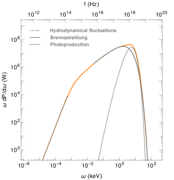
Figure 1: GW power per unit logarithmic frequency, originating from the solar thermal plasma as a function of the frequency, $\omega=2\pi f$.

The solar plasma. We model the Sun as a non-relativistic plasma composed of electrons ($e$) and nucleons ($Z$) following a Maxwell-Boltzmann distribution. We take the corresponding temperature and number density distributions from the B16-GS98 Solar model [13], and estimate the electron density assuming full ionization. Elements heavier than Helium are negligible and are excluded from the analysis.

GWs originate through microscopic and macroscopic mechanisms, respectively corresponding to particle collisions emitting gravitons and GW emission sourced by hydrodynamic fluctuations. The former corresponds to frequencies much larger than that of collisions in the solar plasma, so that there is sufficient time for them not to interfere with each other [14]. Below all collision frequencies of the plasma, fluctuations are large compared with the characteristic microscopic dimensions, allowing a hydrodynamical approach to calculate GW emission [15, 16].

The estimation of the collision frequencies for each species, $\omega^{(i)}_{c}$, is therefore of utmost importance for this work. By following the approach detailed next, we obtain the results presented in Fig. 2. We first calculate the viscosity cross section, $\sigma_{V}$. For instance, for $eZ$,

$$\sigma_{V}^{(eZ)}=\int\frac{\mathrm{d}\sigma}{\mathrm{d}\Omega}^{(eZ)}\sin^{2}\theta\mathrm{d}\Omega\simeq\frac{2\pi\alpha^{2}Z^{2}}{E_{i}^{2}}L_{\text{Coulomb}}\,,$$ (1)

and similarly for $ee$. The collision frequencies are then estimated from the corresponding scattering rate as $\omega^{(e)}_{c}=n_{e}\sigma_{V}^{(ee)}v+\sum_{Z}n_{Z}\sigma_{V}^{(eZ)}v$.

Screening gives rise, in the non-relativistic limit, to an effective Yukawa potential with a range given by the Debye-Hückel screening scale, $\kappa=\left(4\pi\alpha(n_{e}+\sum_{Z}Zn_{Z})/T\right)^{1/2}$ [9], see Fig. 2. For instance, for $eZ$ collisions, $V_{\text{Coulomb}}=-Z\alpha/r\to-Z\alpha e^{-\kappa r}/r$. For non-relativistic collisions, the scattering rate associated with these potentials may be non-perturbative. Nevertheless, in the Sun the scattering largely occurs either in the Born regime, where perturbation theory is applicable, or in the semi-classical regime, where classical physics can be employed. In these cases, the viscosity cross section is given by the last equality in Eq. (1), where the Coulomb logarithm, $L_{\text{Coulomb}}$, equals $\log 2p_{i}/\kappa$ and $\log E_{i}/(Z^{2}\alpha\kappa)$, in the Born and semi-classical approximations, respectively [17, 18].

We note that the collision frequencies should be regarded as transitions scales, particularly because Eq. (1) is valid only up to logarithmic accuracy [19] and different prescriptions exist for the velocity averaging [17]. Here, we follow [14] and take $v$ equal to its thermal average. For further details, see the Appendix.

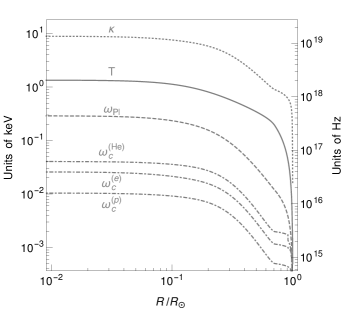
Figure 2: Screening scale (dotted), temperature (solid), plasma frequency (dashed), and collision frequencies (dot-dashed) as a function of distance from the center for the adopted solar model [13]. See text for details.

GWs from hydrodynamical fluctuations. We closely follow Ref. [15] to calculate this contribution. In essence, GWs in this limit are sourced by tensor fluctuations of the energy-momentum tensor, whose Fourier transform is largely independent of the frequency and wave number. Being purely hydrodynamical, the tensor fluctuations are simply proportional to the shear viscosity, $\eta$, of the plasma. Plugging them in Einstein’s Equations, one obtains

$$\frac{\mathrm{d}P}{\mathrm{d}\omega}\Bigg{|}_{\mathrm{Hydrodynamics}}=\frac{16G\omega^{2}}{\pi}\int_{\text{Sun}}\!\!\!\!\mathrm{d}^{3}\mathbf{r}\,\eta T\,.$$ (2)

While this emission has not been previously investigated for the Sun or stellar plasmas, it is known that it contributes to the GW emission from the Early Universe plasma, that is, to the Cosmic Gravitational Microwave Background (CGMB) [15, 20, 21]. The only conceptual difference here is that viscosity must be computed differently because the solar plasma is non-relativistic.

Due to the significant mass ratio between protons and electrons, the primary source of shear viscosity may be attributed to momentum transfer involving protons. For this we note that proton-proton collisions in the Sun are semi-classical. Moreover, the proton component of the solar plasma is not strongly correlated, meaning that the average Coulomb potential energy is much smaller than the thermal energy (which follows from $\alpha\,n_{p}^{1/3}/T\sim 0.03-0.07\ll 1$). This justifies to employ the numerical fits to the state-of-the-art simulations reported by Ref. [22] –more precisely, its Eq. (31)– for the calculation of the viscosity. In practice, this is just a slight modification of the Landau-Spitzer theory, which predicts $\eta\sim m_{p}v_{p}/\sigma^{(pp)}_{V}$ [19]. Let us remark that Eq. (2) loses its validity when the sound waves associated with the hydrodynamical fluctuations are damped by viscosity [23], which happens for $\omega\gtrsim\omega^{(p)}_{c}$ in the one-component approximation.

The solar GW power spectrum from hydrodynamic fluctuations is given by the dashed-dotted line in Fig. 1, where we conservatively put a cut-off for frequencies above $0.05\,\omega_{c}^{(p)}\big{|}_{\rm Center}$ in light of damping.

Collision	$\frac{\mathrm{d}\Gamma}{\mathrm{d}\omega\mathrm{d}V}$
Photoproduction	$n_{\gamma}n_{Z}GZ^{2}\alpha\pi\,\delta(\omega-E_{i})\frac{p_{i}}{\omega}\int\mathrm{d}\!\cos\theta\left(\cot^{2}\!\frac{\theta}{2}[1+\cos^{2}\theta]|F(\theta)|^{2}+{\cal O}(\omega_{\rm Pl}^{2}/\omega^{2})\right)$	$|F(\theta)|^{2}=\frac{\left(2\omega\sin\!\frac{\theta}{2}\right)^{2}}{\kappa^{2}+\left(2\omega\sin\!\frac{\theta}{2}\right)^{2}}$
$\gamma\,Z/e\to Z/e\,h$
Bremsstrahlung	$\frac{32n_{e}n_{Z}GZ^{2}\alpha^{2}p_{i}}{15\omega}\left(\frac{1}{m_{e}}+\frac{1}{m_{Z}}\right)\left(3(1+\xi^{2}){L}+10\xi+{\cal O}(\xi_{s}^{2})\right)$	$\xi=p_{f}/p_{i}$, $\xi_{s}=\kappa/p_{i}$
$eZ\to eZ\,h$		$\omega=E_{i}(1-\xi^{2})$
Bremsstrahlung	$\frac{16n_{e}^{2}G\alpha^{2}p_{i}}{15\omega m_{e}}\left(\left(6(1+\xi^{2})-\frac{3(1-\xi^{2})^{4}+7(1-\xi^{4})^{2}}{2(1+\xi^{2})^{3}}\right){L}+20\xi-\frac{6\xi(1+\xi^{4})}{(1+\xi^{2})^{2}}+{\cal O}(\xi_{s}^{2})\right)$	$L=\log\sqrt{\frac{(1+\xi)^{2}+\xi_{s}^{2}}{(1-\xi)^{2}+\xi_{s}^{2}}}$
$ee\rightarrow ee\ h$

Table 1: Emission rates of gravitons, $h$, from the indicated process in the non-relativistic limit. $p_{i}$ ($p_{f}$) denotes the initial (final) momentum of the colliding particles in the center-of-mass frame, and $E_{i}$ is total kinetic energy.

GWs from particle collisions. This contribution to the solar GW spectrum is obtained by thermally averaging individual graviton emission rates,

$$\frac{\mathrm{d}P}{\mathrm{d}\omega}\Bigg{|}_{\mathrm{Collisions}}=\int_{\text{Sun}}\!\!\!\!\mathrm{d}^{3}\mathbf{r}\,\sum_{i}\omega\left\langle\frac{\mathrm{d}\Gamma^{(i)}(\mathbf{r})}{\mathrm{d}\omega\mathrm{d}V}\right\rangle\,.$$ (3)

The rates entering here are calculated by squaring the relevant amplitudes using CalcHEP [24] and FeynRules [25], and taking the non-relativistic limit for electrons and nucleons. Such rates, at leading order in the screening scale, are summarized in Table 1, while full expressions are reported in the Appendix. We assume spherical symmetry for the integration in the Sun.

Bremsstrahlung. We account for plasma effects following the bremsstrahlung treatment of Ref. [10]. This entails modifying the propagator of the photon exchanged by the charged particles with an effective mass equal to $\kappa$, as suggested by the aforementioned Yukawa potential. In addition to corrections of order $\kappa^{2}/p_{i}^{2}$, this introduces an infrared cut-off. This is essential because, in the absence of screening, the rates exhibit a logarithmic divergence for soft gravitons.

Notably, our explicit computations reveal that the bremsstrahlung rates depend on a common regulating logarithm, which for soft gravitons approaches the one entering the viscosity cross section of Eq. (1). This is not a coincidence, soft theorems [8] arising from basic principles of quantum field theory dictate that $\omega\mathrm{d}\Gamma^{(eZ)}/\mathrm{d}\omega\mathrm{d}V|_{\mathrm{soft}}=(32G/5\pi)E_{i}^{2}\sin^{2}\theta\,n_{e}n_{Z}\sigma^{(eZ)}_{V}v$ for $\omega\ll E_{i}\sim T$, and a similar expression for $ee$ with a factor $1/2$ . Applying this to the center of the Sun is how Weinberg [8, 14] originally found a flat power spectrum, $\mathrm{d}P/\mathrm{d}\omega$, with only a minor logarithmic dependence. Interestingly, despite its quantum-mechanical origin, this formula coincides [14, 27, 28] with the classical emission rate of GWs associated with the quadrupole of the $eZ/ee$ hyperbolic orbit for sufficiently soft radiation .

Weinberg’s calculation motivated studies of bremsstrahlung beyond the soft limit. Reference [30, 31] reported rates associated with $eZ$ –but not $ee$– using similar methods to ours but assuming an infinitely heavy nucleon and no screening. Likewise, bremsstrahlung rates neglecting screening were calculated assuming that the emission comes from one electron moving in the Coulomb potential of a nucleon [32, 33] or another electron [27]. Our results agree with these studies in the appropriate limit .

It is worth mentioning that Ref. [27] calculated $ee$ bremsstrahlung rates in the non-relativistic limit through the following clever insight: photon bremsstrahlung from $ee$ results from their quadrupole, as their dipole vanishes by their indistinguishability, which allows adapting the $ee$ electromagnetic emission to gravitational radiation, with the adjustment being a mere global factor. Our rates, obtained through a different approach, support this conclusion.

Finally, let us remark that our procedure relies on the validity of the Born approximation, which for $ee$ and $eZ$ holds throughout the Sun, except in the outermost regions, approximately the last 15% of the solar radius. Since bremsstrahlung is dominated by processes at the center, neglecting non-perturbative corrections to the graviton emission is justified. The solar GW power spectrum from bremsstrahlung is given by the solid line in Fig. 1, where we put a cut-off for frequencies below $\omega_{c}^{(e)}\big{|}_{\rm Center}$. We remark that for this we use the full rates reported in the appendix, where further details are provided.

Photoproduction. This is analogue to the Primakoff and Compton production of axions. Our results in Table 1 with $\kappa=\omega_{\rm Pl}=0$ coincide with the differential rates for graviton emission reported in Ref. [11]. Nevertheless, from this it is impossible to make sense of the integrated rate, as it diverges due to the collinear divergence appearing at $\theta=0$. To tackle this problem, we again employ insights from axion physics [10]. Concretely, we note that charged particles in the solar plasma mutually interact through their Coulomb fields, leading to a pair correlation function [35, 10, 36]. This gives rise to an effective form factor –$F(\theta)$, in Table 1– that depends on the screening scale $\kappa$ and regularizes the total rate.

If one neglects such correlations and instead consider photons scattering off individual screened charges, one finds the rate given in Table 1, but with $|F(\theta)|\to|F(\theta)|^{2}$ [37]. In practice, this corresponds to modifying the photon propagator with an effective mass, a picture which is appropriate if the scattering process is so slow that the charged particles can move around and rearrange themselves [38]. This issue has been revisited recently for the Primakoff process of axions, accounting for the velocity in the form factor [39]. Despite the differences between axions and gravitons, from this study corrections to the choice given in Table 1 are expected to be negligible.

Note also that the dispersion relation of the initial-state photon is influenced by the surrounding plasma, which imparts an effective mass to transverse photons equal to the plasma frequency, $\omega_{\mathrm{Pl}}=\left(4\pi n_{e}\alpha/m_{e}\right)^{1/2}$. However, since the solar temperature far exceeds it (see Fig. 2), the GW spectrum remains largely insensitive to the photon’s effective mass, a fact we have verified explicitly. The main consequence is the phase-space factor $p_{i}/\omega$, that provides a lower cut-off to the photoproduction contribution at each point of the Sun. We note that this is completely analogous to the Primakoff effect for axions, which we discuss in the appendix for completeness. It is noteworthy that Ref. [12] calculated photoproduction rates using semi-classical methods and including the effect of the plasma frequency, but did not account for screening, which is the dominant effect.

The resulting solar GW power spectrum from photoproduction is given by the dashed line in Fig. 1.

Transition regime and other processes. As it shifts from macroscopic to microscopic fluctuations, $\mathrm{d}P/\mathrm{d}\omega$ transitions from $\propto\omega^{2}$ to $\propto\omega^{0}$ within the range $\omega^{(p)}_{c}\lesssim\omega\lesssim\omega^{(e)}_{c}$. Similar to the case of the CGMB, a thorough examination of this regime necessitates a hydrodynamical simulation. Nevertheless, we postulate an interpolating factor $\omega^{2}/(\omega^{2}+\omega_{0}^{2})$. Eqs. (2)-(3) and the Landau-Spitzer viscosity for protons give $\omega_{0}\approx(\omega^{(p)}_{c}\omega^{(e)}_{c})^{1/2}\propto 1/\eta$. Notably, the interpolating factor with the predicted scale $\omega_{0}\propto 1/\eta$ is also found in analytical studies of the energy-momentum tensor for relativistic plasmas (in the so-called shear channel) [15]. It is also worth mentioning that power shifts from $\mathrm{d}P/\mathrm{d}\omega\propto\eta\sim 1/\sigma_{V}$ to soft bremsstrahlung, where $\mathrm{d}P/\mathrm{d}\omega\propto\sigma_{V}$. Interestingly, the same behavior is found for the CGMB because $\sigma_{V}\sim\alpha^{2}/T^{2}$. Our interpolation of the solar GW power spectrum between the hydrodynamic and bremsstrahlung regime is given by the orange solid line in Fig. 1.

We might consider other emission processes known to exist for axions, including small features associated with atomic emission lines [40, 41] as well as photoproduction exploiting the solar magnetic field at frequencies $\omega_{\mathrm{Pl}}$ [42, 43, 44, 39], i.e. from longitudinal photons. However, we emphasize that gravitons exhibit a unique coupling to photons and fermions indicating fixed proportions for the different contributions of the solar spectrum. In contrast, axions possess model-dependent couplings to photons and fermions, allowing scenarios where bremsstrahlung is subdominant compared to photoproduction processes induced by the solar magnetic field. In the light of this, the latter hardly contribute to the GW spectrum around $\omega_{\mathrm{Pl}}\sim 0.3\,\mathrm{keV}$ or lower where bremsstrahlung dominates by more than five orders of magnitude.

As explained above, similar to axions, the emission rates of gravitons from atomic levels can be derived by multiplying ordinary atomic transition rates by a global factor, see e.g. Refs. [45, 46]. Being quadrupole transitions, these are largely suppressed in comparison to those induced by dipole terms, to which axions couple [40, 41], and hence we neglect them.

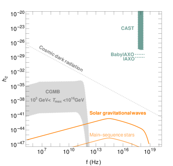
Figure 3: Characteristic GW strain versus frequency. Exclusion bound and corresponding projected sensitivities of current (CAST) and future (BabyIAXO, IAXO) axion helioscopes, together with the corresponding predictions from the solar GW spectrum in Fig. 1, an estimate of the stochastic background from the main-sequence stars in the Milky Way, the CGMB spectrum, and the bound from the total radiation in the Universe.

Discussion and outlook. Our interpolation of the solar GW power spectrum including all processes is presented in Fig. 1. In terms of power, the relative contribution of each process is as follows: 25% for photoproduction, 33% for $ee$ bremsstrahlung, 24% for $ep$ bremsstrahlung, 17% for $eHe$ bremsstrahlung, with the rest attributed to the hydrodynamical contribution.

Axion helioscopes [47] can be used as detectors of gravitational radiation exploiting the inverse Gertsenshtein effect [48, 49], by which GWs convert to electromagnetic waves in the presence of an external magnetic field. Reference [50] presented an exclusion bound from CAST [51], sensitivity prospects for IAXO [52], and compared them against Weinberg’s prediction of the solar GW spectrum. In Fig. 3 we present their findings in terms of the GW strain, $h_{c}\equiv 2(G\,\mathrm{d}P/\mathrm{d}\omega)^{1/2}/d_{\rm Sun}\omega^{1/2}$, together with the complete spectrum as derived from Fig. 1. For comparison, we also display the CGMB, whose overall normalization depends upon the (unknown) maximum temperature of the primordial plasma [21]. In addition, we show the cosmic dark radiation bound, arising from the fact that GWs contribute to the energy budget of the Universe in the form of radiation and are thus limited by Big Bang Nucleosynthesis (BBN) and Cosmic Microwave Background (CMB) observations [7]. In addition, we derive also prospects for BabyIAXO following Refs. [21, 52]. For further comparison, we include an estimate of the stochastic background associated with main-sequence stars in the galaxy. Noting that these stars have similar masses to the Sun [53], we approximate their GW spectrum using the one of the Sun, leading to $h_{c\,\text{stars}}=\sqrt{\int dV\,n_{\text{stars}}\,d^{2}_{\rm Sun}/d^{2}}\,h_{c\,\text{Sun}}$. A similar estimation has been performed in Ref. [54] for stellar neutrinos. Adapting their results for the ${}^{7}\mathrm{Be}$ line, we find $h_{c\,\text{stars}}\sim 10^{-4}h_{c\,\text{Sun}}$. We note that this figure should be regarded as an order-of-magnitude estimate.

Our calculation of solar GWs reveals a clear similarity between gravitons and axions. Expanding on this idea, we could consider the emission of massive spin-2 particles from the Sun, which could also constitute the dark matter of the Universe, see e.g. [55, 56, 57]. Extending the methods discussed here to such particles, we find that the resulting spectrum is nearly identical to that of the solar GWs, differing only by an overall factor associated with the coupling of spin-2 particles to SM fields. In a separate publication [58], we will discuss this synergy and present observational prospects at helioscopes.

Our study represents a step towards establishing a multi-frequency GW background from SM processes, similar to that of neutrinos [59]. In fact, our approach can be extended to other stellar plasmas  and to the early stages of the Universe after nucleosynthesis, where plasmas are also non-relativistic. Figure 3 indicates that current experiments are still many orders of magnitude away from detecting signals from these backgrounds. Whether we can aspire to probe such strain sensitivities in the future remains an open question.

Acknowledgements. We thank Diego Blas, Andrea Caputo, Valerie Domcke, Javier Galán, Maurizio Giannotti, Igor Irastorza, Mikko Laine, Jamie McDonald, Maxim Pospelov and Georg Raffelt for discussions. CGC is supported by a Ramón y Cajal contract with Ref. RYC2020-029248-I, the Spanish National Grant PID2022-137268NA-C55 and Generalitat Valenciana through the grant CIPROM/22/69. A.R. acknowledges support by the Deutsche Forschungsgemeinschaft (DFG, German Research Foundation) under Germany’s Excellence Strategy - EXC 2121 Quantum Universe - 390833306 and under - 491245950. This article is based upon work from COST Action COSMIC WISPers CA21106, supported by COST (European Cooperation in Science and Technology).

Appendix A Viscosity cross sections in the Born and semi-classical regimes

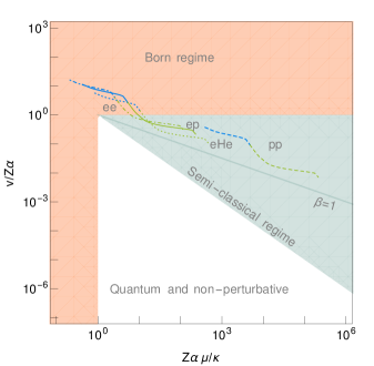
Figure S1: Scattering regimes of the indicated solar collisions due to the screened Coulomb potential. Perturbation theory is applicable in the Born regime, while classical physics is valid in the semi-classical regime. Different points correspond to various distances from the center of the Sun. See the text for details.

Viscosity cross sections can be used to estimate collision frequencies, and as discussed in the main text, Weinberg’s soft theorem relates them to graviton bremsstrahlung. Hence, they are of utmost importance for this work. They are defined by

$$\sigma_{V}^{(ab)}=\int\frac{\mathrm{d}\sigma}{\mathrm{d}\Omega}^{(ab)}\sin^{2}\theta\,\mathrm{d}\Omega\,.$$ (S1)

For a Coulomb potential, $V(r)=-Z_{a}Z_{b}\alpha/r$, between two particles of charge $Z_{a}$ and $Z_{b}$ (in units of $e$), this cross section logarithmically diverges, because the corresponding $\mathrm{d}\sigma^{(ab)}/{\mathrm{d}\Omega}$ scales as $1/\sin^{4}(\theta/2)$. This is not really a problem because the Coulomb potential is screened. In the non-relativistic limit, this is described by an effective Yukawa potential with a range given by the Debye-Hückel screening scale,

$$V(r)=-\frac{Z_{a}Z_{b}\alpha}{r}e^{-\kappa r}\,, \kappa^{2}=\frac{4\pi\alpha}{T}\left(n_{e}+\sum_{Z}Zn_{Z}\right)\,.$$ and (S2)

Determining $\mathrm{d}\sigma^{(ab)}/{\mathrm{d}\Omega}$ for non-relativistic particles interacting by means of such a potential is non-trivial due to non-perturbative effects. Nevertheless, as we show in the sequel, for the relevant collisions in the Sun the scattering largely occurs either in the Born regime, where perturbation theory is applicable, or in the weakly coupled semi-classical regime, where classical physics can be employed. In both scenarios, one obtains

$$\sigma_{V}^{(ab)}\simeq\frac{2\pi\alpha^{2}Z_{a}^{2}Z_{b}^{2}}{E_{i}^{2}}L_{\text{Coulomb}}\,,$$ (S3)

where $L_{\text{Coulomb}}$ is the Coulomb logarithm. We emphasize this is valid to logarithmic accuracy, meaning that this expressions neglects quantities smaller than $L_{\text{Coulomb}}$. For a comprehensive discussion see e.g. Ref. [19]. The Born regime applies for large velocities, namely $Z\alpha\ll v$, or for sufficiently small couplings, concretely $Z\alpha\ll\kappa/\mu$ [19], where $\mu$ is the reduced mass. Ordinary quantum perturbation theory employing the potential in Eq. (S2) gives 

$$L_{\text{Coulomb}}=\log\left(\frac{2\mu v}{\kappa}\right)\,.$$ (S4)

The semi-classical regime takes place when the de Broglie wavelength is much smaller than the range of the potential, that is, $\kappa\ll\mu v$  [19]. In this case there is a critical parameter, $\beta=|Z_{a}||Z_{b}|\kappa\alpha/\mu v^{2}$, determining different sub-regimes [18]. For $\beta\ll 1$, of interest in this work, the plasma is weakly-coupled and the Coulomb logarithm is given by [19, 18]

$$L_{\text{Coulomb}}=\log\left(\frac{\mu v^{2}}{|Z_{a}||Z_{b}|\alpha\kappa}\right)\,.$$ (S5)

The range of applicability of either regime along the position in the Sun is sketched in Fig. S1. The green portion of the lines corresponds to the 15% outermost part, while the blue part corresponds to the innermost 85%. For simplicity we only show $ee$, $ep$, $eHe$ and $pp$ collisions. We also show the line $\beta=1$, above which the plasma is weakly coupled and Eq. (S5) can be used. Note that pp collisions are semi-classical, as mentioned in the main text.

Appendix B Graviton emission rates and Feynman rules

The emission rate per unit volume of one graviton in the collision of two particles is given by

$$\frac{d\Gamma}{\mathrm{d}\omega\mathrm{d}V}\left(1+2\rightarrow h_{\lambda}\cdots\right)=\int dn_{1}dn_{2}|{\cal M}(\lambda)|^{2}{\rm d(PS)}(2\pi)^{4}\delta^{(4)}\left(p_{1}+p_{2}-p-\sum_{k}p_{k}\right)\,,$$ (S6)

where $p=(\omega,\bf{p})$ and $\lambda$ are respectively the graviton momentum and helicity, while ${\rm d(PS)}$ is the phase space associated with the final-state particles,

$${\rm d(PS)}=\frac{\omega^{2}{\rm d}\Omega_{\bf{p}}}{(2\pi)^{3}2\omega}\prod_{k}\frac{{\rm d}^{3}p_{k}}{(2\pi)^{3}2E_{k}}\,.$$ (S7)

In addition, ${\cal M}(\lambda)$ is the graviton emission amplitude, which can be cast as

$${\cal M}(\lambda)={\cal M}_{\mu\nu}\epsilon^{\mu\nu}_{(\lambda)}(p)\,,$$ (S8)

where polarizations tensors are given by

$$\epsilon^{\mu\nu}_{\pm 2}(p)=\epsilon_{\pm}^{\mu}(p)\epsilon_{\pm}^{\nu}(p)\,, \epsilon_{\pm}^{\mu}(p)=\frac{1}{\sqrt{2}}\left(\begin{array}[]{c}0\\ \mp\cos\theta\cos\phi+i\sin\phi\\ \mp\cos\theta\sin\phi-i\cos\phi\\ \pm\sin\theta\end{array}\right)\,, p^{\mu}=\left(\begin{array}[]{c}\omega\\ |\bf{p}|\sin\theta\cos\phi\\ |\bf{p}|\sin\theta\sin\phi\\ |\bf{p}|\cos\theta\end{array}\right)\,.$$ with and (S17)

When perturbation theory applies, ${\cal M}_{\mu\nu}$ in Eq. (S6) can be calculated from tree-level diagrams, with the vertices obtained from

$$\mathcal{L}=\frac{1}{2}\partial_{\rho}h_{\mu\nu}\partial^{\rho}h^{\mu\nu}-\frac{1}{2}\partial_{\rho}h\partial^{\rho}h+\partial_{\rho}h\partial_{\nu}h^{\rho\nu}-\partial_{\rho}h_{\mu\nu}\partial^{\nu}h^{\mu\rho}+\frac{1}{2}\kappa_{G}\,h_{\mu\nu}T^{\mu\nu}\,,$$ (S18)

where $T^{\mu\nu}$ is the stress-energy-momentum tensor of the Standard-Model particles, and $g_{\mu\nu}=\eta_{\mu\nu}+\kappa_{G}h_{\mu\nu}$ with $\kappa_{G}=\sqrt{32\pi G}$. The corresponding Feynman rules of relevance for this work are $C^{\rm(fermion)}_{\mu\nu}(p_{1},p_{2})=\frac{i}{8}\kappa_{G}\left[2\eta_{\mu\nu}(\not{p}_{1}+\not{p}_{2}-2m_{f})-(p_{1}+p_{2})_{\mu}\gamma_{\nu}-\gamma_{\mu}(p_{1}+p_{2})_{\nu}\right]\,,$    $C^{\rm(photon)}_{\alpha\beta\mu\nu}(p_{1},p_{2})=-\frac{i}{2}\kappa_{G}\left[\eta_{\mu\nu}\eta_{\alpha\beta}\,p_{1}\cdot p_{2}-\eta_{\mu\nu}p_{1\beta}p_{2\alpha}+\eta_{\nu\alpha}p_{1\beta}p_{2\mu}-\eta_{\alpha\beta}p_{1\nu}p_{2\mu}+\eta_{\mu\beta}p_{1\nu}p_{2\alpha}\right.$ $\qquad\qquad\qquad\left.-\eta_{\nu\alpha}\eta_{\mu\beta}p_{1}\cdot p_{2}+\eta_{\nu\beta}p_{1\mu}p_{2\alpha}-\eta_{\alpha\beta}p_{1\mu}p_{2\nu}+\eta_{\mu\alpha}p_{1\beta}p_{2\nu}-\eta_{\nu\beta}\eta_{\mu\alpha}p_{1}\cdot p_{2}\right]\,,$   $C^{\rm(quartic)}_{\alpha\mu\nu}=-\frac{i}{4}eZ\kappa_{G}\left[2\eta_{\mu\nu}\gamma_{\alpha}-\eta_{\alpha\mu}\gamma_{\nu}-\eta_{\alpha\nu}\gamma_{\mu}\right]\,.$

The fermion line is either $e$ or $Z$. These rules agree with existing literature (see e.g. [66, 67]), and were derived implementing Eq. (S18) in FeynRules [25]. This process also gives the input needed by CalcHEP [24] for cross section calculations. Using Package-X [68], we manipulate the symbolic output thus obtained to compute ${\cal M}^{\mu\nu}$. For all processes, we verify that

$$p^{\mu}{\cal M}_{\mu\nu}=0\,,$$ (S19)

as follows from energy-momentum conservation.

Validity of the Born approximation. The procedure just described relies on the validity of the Born approximation, which holds true for photoproduction, $\gamma a\to ah$, but becomes problematic for bremsstrahlung processes, $ab\to ab\,h$. (Here $a$ or $b$ stands for an electron or a nucleon, as above). Let us discuss bremsstrahlung first. This issue is closely connected to the perturbativity in the $ab$ collisions, discussed above. This can be understood as follows. The Born approximation assumes that particles in the initial and final states are approximately described by plane waves. While this assumption holds true for gravitons, it does not necessarily apply to electrons or nucleons, as they are subject to mutual interaction. The extent to which a plane wave is a good approximation depends on whether this mutual interaction is perturbative. If it is, the wave function of electrons or nucleons can be expanded perturbatively, resulting in a plane wave with a small additional contribution, whose impact on the scattering rate appears beyond the Born approximation.

The previous argument makes it clear that whenever perturbativity is a problem for graviton bremsstrahlung, it is also a problem for the bremsstrahlung of axion or photons. Interestingly, Weinberg has recently revisited the latter case, providing approximation formulas for photon bremsstrahlung valid beyond the Born approximation [17] (see also Ref. [69]). Such formulas arise from the non-perturbative wave functions and provide substantial corrections when $v/Z\alpha$ is small. In light of Fig. S1, this shows that for the main processes contributing to graviton bremsstrahlung in the Sun –namely, $ee$, $ep$ and $eHe$– the Born approximation works well except in the last 15% of the solar radius. There, the temperature is comparatively lower resulting in $v/Z\alpha<1$, invalidating the plane-wave assumption. Since bremsstrahlung is dominated by processes at the center, neglecting non-perturbative corrections to the graviton emission is justified. Likewise, this argument applies to axion bremsstrahlung, where accounting for non-perturbative wave functions gives corrections below 10% (see e.g. Ref. [39]).

Finally, the aforementioned argument justifies the use of the Born approximation for photoproduction because the charged particles in the initial state, although non-relativistic, do not experience a distortion of their wave function, as in the case of bremsstrahlung.

B.1 Photoproduction

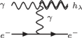
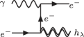
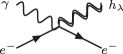
Figure S2: Feynman diagrams for photoproduction

Having justified the Born approximation, let us note that diagrammatically such collisions correspond to Feynman diagrams where the photon emits $h_{\pm 2}$ and then collides with a charged particle (Primakoff-like scattering), or to one photon impinging on a charged particle that subsequently emits $h_{\pm 2}$ (Compton-like scattering), or to a diagram involving a contact interaction with all particles. Using Eq. (S7), the amplitude can be cast as

$${\cal M}_{\alpha\beta}=\overline{u}_{3}\Gamma_{\alpha\beta\mu}u_{2}\,\epsilon^{\mu}(p_{1})\,,$$ (S20)

where the subscripts $2$ and $3$ refer to the fermion in the initial and final state, respectively, while $1$ refers to the incoming photon. Following the procedure outlined above, we find

$$\Gamma_{\alpha\beta\mu}= - \frac{Ze}{(p_{2}-p_{3})^{2}}C_{\mu\lambda\alpha\beta}^{\rm(photon)}(p_{1},p_{3}-p_{2})\gamma^{\lambda}$$

$$+ \frac{Ze}{(p_{1}+p_{2})^{2}-m_{f}^{2}}C^{\rm(fermion)}_{\alpha\beta}(p_{1}+p_{2},p_{3})\left(\not{p_{1}}+\not{p_{2}}+m_{f}\right)\gamma_{\mu}$$

$$+ \frac{Ze}{(p_{1}-p_{3})^{2}-m_{f}^{2}}\gamma_{\mu}\left(-\not{p_{1}}+\not{p_{3}}+m_{f}\right)C^{\rm(fermion)}_{\alpha\beta}(p_{2},-p_{1}+p_{3})$$

$$+ C^{\rm(quartic)}_{\mu\alpha\beta}\,.$$

In addition to making sure that this satifies Eq. (S19), we also verify gauge invariance by means of the Ward–Takahashi relation

$$p_{1}^{\mu}\,\left(\overline{u}_{3}\Gamma_{\alpha\beta\mu}u_{2}\,\epsilon^{\alpha\beta}_{(\lambda)}(p)\right)=0\,.$$ (S22)

Plugging Eq. (B.1) into Eq. (S6), we obtain the photoproduction rates. Taking the non-relativistic limit, $m_{f}\gg\omega$, we obtain the differential emission rate

$$\frac{\mathrm{d}\Gamma}{\mathrm{d}\omega\mathrm{d}V\mathrm{d}\Omega}\left(\gamma Z\to Z\,h\right)=n_{\gamma}n_{Z}\delta(\omega-p_{i})\,Z^{2}\frac{\mathrm{d}\sigma}{\mathrm{d}\Omega}\bigg{|}_{e}\,, \frac{\mathrm{d}\sigma}{\mathrm{d}\Omega}\bigg{|}_{e}=\frac{1}{2}\,\alpha G\,\cot^{2}\!\frac{\theta}{2}\left(1+\cos^{2}\theta\right)\,.$$ with (S23)

This cross section was reported in Ref. [37, 11]. As usual, here $\theta$ is the scattering angle in the photoproduction process, i.e. the angle between the graviton and the incoming particles. So far, we have assumed that the photon is massless. However, the surrounding plasma gives photons in the external line an effective mass given by the plasma frequency, $\omega_{\rm pl}$. A similar modification is required in the photon propagator and vertices. Nevertheless, the solar temperature far exceeds $\omega_{\rm pl}$ (see Fig. 2), allowing us to calculate photoproduction rates by expanding on $\omega_{\rm pl}$. In practice, this approach is effectively equivalent to treating the external photon as massless while incorporating the plasma frequency into the phase space, as reported in the Table 1 with $\kappa=0$. The resulting cross section agrees with semi-classical calculations [12] accounting for a non-trivial dispersion (without screening).

As is clear from Eq. (S23), the total rate diverges due to the pole at $\theta=0$. The origin of the divergence is the photon propagator in the amplitude of the Primakoff-like diagram, whose denominator $-(p_{2}-p_{3})^{2}$ equals in the non-relativistic limit the square of the three-momentum transfer, $|{\bf q}|=2\omega\sin(\theta/2)$. To gain further intuition on this, let us discuss the case of axions, where a similar divergence occurs for the Primakoff effect. As shown in [10], the divergence is effectively regularized by accounting for correlations among plasma particles. This is closely related to screening, and despite the differences between axions and gravitons, the same remains true for the latter in non-relativistic limit, $m_{f}\gg\omega$. We repeat the argument here for completeness.

In the non-relativistic limit, $|{\bf q}|/m_{f}\ll 1$, and therefore the charged particles off which the photon scatters may be regarded as at rest during the collision. As a result, the photon scatters off a charge distribution, $\rho({\bf r})$, with a cross section

$$\frac{\mathrm{d}\sigma}{\mathrm{d}\Omega}=\frac{\mathrm{d}\sigma}{\mathrm{d}\Omega}\bigg{|}_{e}\left|F(\mathbf{q})\right|^{2}\,, F({\bf q})=\frac{1}{e}\int\mathrm{d}{\bf r}\,e^{i{\bf q}\cdot{\bf r}}\rho({\bf r})\,.$$ where (S24)

The cross section with subscript $e$ refers to electrons as introduced in Eq. (S23). For $N$ point charges $Z_{i}e$ located at $\mathbf{r}_{i}$, a explicit computation shows that $F({\bf q})=\sum_{i}^{N}Z_{i}e^{i{\bf q}\cdot{\bf r}_{i}}$ as well as $\left|F(\mathbf{q})\right|^{2}=\sum_{i}^{N}Z_{i}^{2}+\sum_{\begin{subarray}{c}i\neq j\end{subarray}}^{N}Z_{i}Z_{j}\cos\left(\mathbf{q}\cdot\mathbf{r}_{ij}\right)$ where $\mathbf{r}_{ij}\equiv\mathbf{r}_{i}-\mathbf{r}_{j}$. This must be averaged accounting for the statistical ensemble describing the plasma. Clearly, the first term is associated with individual charges, while the second one describes interference effects. The latter averages to zero for very diluted plasmas ($\kappa\to 0$) because their particles are uncorrelated. In that case, the total rate in Eq. (S24) simply consists of adding the contribution of individual charges. Nevertheless, in real plasmas particles mutually interact through their Coulomb fields and their motion is slightly correlated. Concretely, the potential, $\phi_{i}$, around a given particle is sourced by a charge cloud with density

$$\rho_{i}(r)=Z_{i}e\left(\delta^{3}(\mathbf{r})-\frac{\kappa^{2}}{4\pi}\frac{e^{-\kappa r}}{r}\right)=-\nabla^{2}\phi_{i}\,.$$ (S25)

That is, the Coulomb field of any charge is screened over distances larger than about $\kappa^{-1}$. To determine the aforementioned average, and hence the effect of correlations, we note that the potential energy associated with Eq. (S25) is given by $U=\frac{1}{2}e\sum^{N}_{i\neq j}Z_{i}\phi_{i}$. Employing the Boltzmann factor associated with this potential energy, $e^{-U/T}$, at leading order in $\alpha$ one finds that thermal average is

$$\sum^{N}_{j\neq i}Z_{j}\langle\cos\left(\mathbf{q}\cdot\mathbf{r}_{ij}\right)\rangle=-\frac{Z_{i}\kappa^{2}}{\kappa^{2}+|{\bf q}|^{2}}\,, \left\langle\left|F(\mathbf{q})\right|^{2}\right\rangle=\sum_{i=1}^{N}Z_{i}^{2}\left(1-\frac{\kappa^{2}}{\kappa^{2}+|\mathbf{q}|^{2}}\right)\,.$$ which leads to (S26)

Hence, Eq. (S24) implies that [10]

$$\left\langle\frac{\mathrm{d}\sigma}{\mathrm{d}\Omega}\right\rangle=\sum_{i=1}^{N}Z_{i}^{2}\frac{\mathrm{d}\sigma}{\mathrm{d}\Omega}\bigg{|}_{e}\frac{|\mathbf{q}|^{2}}{\kappa^{2}+|\mathbf{q}|^{2}}\,.$$ (S27)

In summary, one must add individual cross sections introducing a global factor determined by the screening scale. This clearly regularizes the divergence at $|{\bf q}|=0$. Following this procedure, we obtain the rates reported in Table 1. A few comments are in order.

While the Compton process for axions arises from a renormalizable coupling, $g_{aee}$, leading to a cross section independent of the momentum transfer in the non-relativistic limit, the Primakoff process results from a non-renormalizable coupling, $g_{a\gamma\gamma}$, and leads to a differential cross section scaling as the fourth power of the momentum transfer [10]. Thus, only the latter exhibits a divergence, raising the question of whether the Compton-like and Primakoff-like diagrams for gravitons must be separated somehow. Nonetheless, unlike photoproduction of axions, where such a separation is feasible, for gravitons that cannot be done in a meaningful manner. First, because they depend on the same coupling, namely, the gravitational coupling in Eq. (S18). Moreover, although the identity in Eq. (S22) is separately satisfied by the Compton-like diagrams of Fig. S2, that is not the case of the identity associated with energy-momentum conservation, Eq. (S19). In the light of this, we apply Eq. (S27) to photoproduction of gravitons as a whole.

One might ignore the correlations given by Eq. (S26) and assume that the incoming photon scatters off a single charge distribution given by Eq. (S25). This is the regularization advocated by Ref. [37]. The resulting cross section is that in Eq. (S27) with $|\mathbf{q}|^{2}/(\kappa^{2}+|\mathbf{q}|^{2})\to|\mathbf{q}|^{4}/(\kappa^{2}+|\mathbf{q}|^{2})^{2}$. As explained in the main text, this issue has been revisited recently for the Primakoff process [39], accounting for the velocity in the form factor. Corrections to Eq. (S27) have been deemed negligible. Coupled with this, let us remark that, as opposed to bremsstrahlung or two-two scattering, the effect of screening here cannot be understood as an effective mass for the photon for several reasons. First, the effective mass of transverse photons in the external line is given by the plasma frequency, $\omega_{\rm pl}$, and not by the Debye-Hückel screening scale, $\kappa$, which in the Sun satisfies $\omega_{\rm pl}\ll\kappa$. See Fig. 2. In fact, even if one adopts an ad-hoc prescription in which the virtual photon in Fig. S2 has a mass $\kappa$, while the incoming external photon has a mass $\omega_{\rm pl}$, one quickly finds inconsistencies. For instance, this approach spoils Eq. (S19).

B.2 Bremsstrahlung

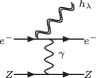
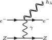
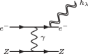
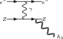
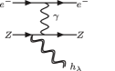
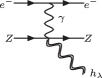
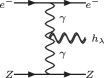
Figure S3: Feynman diagrams for bremsstrahlung in $eZ$ collisions.

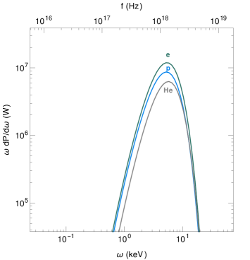
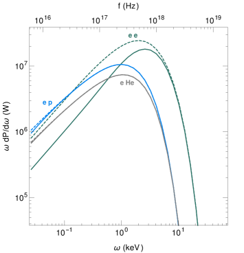
Figure S4: Left: Contribution of photoproduction processes to the solar GW spectrum. Right: Contribution of bremsstrahlung processes to the solar GW spectrum. Solid lines are the full results determined by Eqs. (B.2) and  (S29). The dashed lines are the leading results in the screening scale, reported in Table 1.

In the Born approximation, there are seven Feynman diagrams associated with bremsstrahlung in $eZ$ collisions, see Fig. S3. For $ee$ collisions, additional diagrams are obtained by symmetrizing the final state of those shown in Fig. S3. Note that bremsstrahlung from two-nucleon states are negligible. To calculate the corresponding $M^{\mu\nu}$, we follow the procedure outlined above. Concretely, we manipulate the symbolic output provided by CalcHEP [24] using Package-X [68]. Crucially, we verify that Eq. (S19) is satisfied. Subsequently, we use this together with the appropriate polarization tensors to compute ${\cal M}(\lambda)$. To account for screening, we modify the photon propagators with an effective mass equal to the screening scale. As argued above, that is the correct prescription for slow particles such as the non-relativistic plasma components (in contrast to the external photon in the photoproduction process described above). From this, we calculate the differential cross sections in energy. To the best of our knowledge, the expression for these have never been reported in the literature in a general form. This is not surprising as the aforementioned procedure is a daunting task, even in the the non-relativistic limit. After algebraic manipulation, in such a limit we find

$$\frac{{\mathrm{d}}\sigma\!v}{{\mathrm{d}}\omega}\Bigg{|}_{eZ\to eZ\,h} = \frac{32Z^{2}\alpha^{2}Gp_{i}}{15\omega}\left(\frac{1}{m_{e}}+\frac{1}{m_{Z}}\right)\left[3(1+\xi^{2}+\xi_{s}^{2})L\right.$$

$$\left.+10\xi+\frac{1}{3}\xi_{s}^{2}\left(\frac{(1-\xi)^{2}\left(18(1+\xi)^{4}+29(1+\xi)^{2}\xi_{s}^{2}+12\xi_{s}^{4}\right)}{\left((1+\xi)^{2}+\xi_{s}^{2}\right)^{3}}-(\xi\to-\xi)\right)\right]\,,$$

with notation $L$, $\xi$ and $\xi_{s}$ introduced in Table 1. In this calculation we do not take the limit $m_{Z}\gg m_{e}$, we simply assume that both nucleons and electrons are non-relativistic. Likewise

$$\frac{{\mathrm{d}}\sigma\!v}{{\mathrm{d}}\omega}\Bigg{|}_{ee\to ee\,h}=\frac{32\alpha^{2}Gp_{i}}{15\omega m_{e}}\left\{20\xi-\frac{6\xi(1+\xi^{4})}{(1+\xi^{2})^{2}}+\left[6(1+\xi^{2})-\frac{3(1-\xi^{2})^{4}+7(1-\xi^{4})^{2}}{2(1+\xi^{2})^{3}}\right.\right.$$ (S29)

$$\left.\left.\frac{1}{2}\xi_{s}^{2}\left(\frac{6(\xi^{4}+1)(1-\xi^{2})^{2}}{(\xi^{2}+1)^{2}(\xi^{2}+\xi_{s}^{2}+1)^{2}}+\frac{2(\xi^{4}-4\xi^{2}+1)(1-\xi^{2})^{2}}{(\xi^{2}+1)(\xi^{2}+\xi_{s}^{2}+1)^{3}}+\frac{13\xi^{8}+22\xi^{4}+13}{(\xi^{2}+1)^{3}(\xi^{2}+\xi_{s}^{2}+1)}+15\right)\right]L\right.$$

$$+\left.\xi_{s}^{2}\left[2(1-\xi^{2})^{2}\left(-\frac{(1-\xi)^{4}-80\xi^{2}}{16\,\xi^{2}(\xi+1)^{2}((\xi+1)^{2}+\xi_{s}^{2})}-\frac{3(\xi^{4}+1)\xi_{s}^{2}+4(\xi^{6}+1)}{8\xi(\xi^{2}+1)^{2}(\xi^{2}+\xi_{s}^{2}+1)^{2}}+\frac{6(\xi+1)^{2}+5\xi_{s}^{2}}{3((\xi+1)^{2}+\xi_{s}^{2})^{3}}\right)\right.\right.$$

$$\left.\left.-(\xi\to-\xi)\right]\right\}\,.$$

For $\xi_{s}=0$, these cross sections agree fully with those reported by Gould in Refs. [33, 27]. The total emission rate is given by

$$\frac{\mathrm{d}\Gamma}{\mathrm{d}\omega\mathrm{d}V}\Bigg{|}_{\rm Bremsstrahlung}=\frac{1}{2}n_{e}^{2}\frac{{\mathrm{d}}\sigma\!v}{{\mathrm{d}}\omega}\Bigg{|}_{ee\to ee\,h}+\sum_{Z}n_{e}n_{Z}\frac{{\mathrm{d}}\sigma\!v}{{\mathrm{d}}\omega}\Bigg{|}_{eZ\to eZ\,h}\,.$$ (S30)

The partial contributions of each channel are shown in Fig. S4. To leading order in the screening scale the resulting expressions are reported in Table 1. While these approximations are quite accurate for $eZ$ bremsstrahlung, they are less precise for $ee$ bremsstrahlung, as shown in Fig. S4. This underscores the critical importance of incorporating screening effects in the bremsstrahlung rates.

Soft emission. Let us consider the initial state $eZ$. A soft graviton leads to $\xi\to 1$. Taking $\xi_{s}\to 0$, the effect of screening appears only in the logarithm with $L\to L_{\rm Coulomb}$, and the corresponding emission rate can be cast as

$$\frac{\mathrm{d}\Gamma}{\mathrm{d}\omega\mathrm{d}V}\Bigg{|}_{eZ\to eZ\,h}=\frac{64\alpha^{2}Z^{2}Gv}{5}L_{\rm Coulomb}n_{e}n_{Z}=\frac{8G}{5\pi}n_{e}n_{Z}\,\mu^{2}v^{5}\sigma_{V}^{(eZ)}\,.$$ (S31)

In the last equation, we use the viscosity cross section obtained in Eq. (S3) with $E_{i}=\mu v^{2}/2$. Note that $v=p_{i}\left(\frac{1}{m_{e}}+\frac{1}{m_{Z}}\right)$. Similarly, for $ee$ Eq. (S29) reduces to

$$\frac{\mathrm{d}\Gamma}{\mathrm{d}\omega\mathrm{d}V}\Bigg{|}_{ee\to ee\,h}=\frac{32\alpha^{2}Z^{2}Gv}{5}L_{\rm Coulomb}n_{e}^{2}=\frac{4G}{5\pi}n_{e}^{2}\,\mu^{2}v^{5}\sigma_{V}^{(ee)}\,.$$ (S32)

Here $v=2p_{i}/m_{e}$. As explained in the text, this was first proven by Weinberg [8], who used it to estimate the total power emitted by the Sun.

References

- [1] LIGO Scientific, Virgo Collaboration, B. P. Abbott et al., “GW170817: Observation of Gravitational Waves from a Binary Neutron Star Inspiral,” Phys. Rev. Lett. 119 no. 16, (2017) 161101, arXiv:1710.05832 [gr-qc].
- [2] LIGO Scientific, Virgo Collaboration, B. P. Abbott et al., “Observation of Gravitational Waves from a Binary Black Hole Merger,” Phys. Rev. Lett. 116 no. 6, (2016) 061102, arXiv:1602.03837 [gr-qc].
- [3] EPTA, InPTA: Collaboration, J. Antoniadis et al., “The second data release from the European Pulsar Timing Array - III. Search for gravitational wave signals,” Astron. Astrophys. 678 (2023) A50, arXiv:2306.16214 [astro-ph.HE].
- [4] D. J. Reardon et al., “Search for an Isotropic Gravitational-wave Background with the Parkes Pulsar Timing Array,” Astrophys. J. Lett. 951 no. 1, (2023) L6, arXiv:2306.16215 [astro-ph.HE].
- [5] NANOGrav Collaboration, G. Agazie et al., “The NANOGrav 15 yr Data Set: Evidence for a Gravitational-wave Background,” Astrophys. J. Lett. 951 no. 1, (2023) L8, arXiv:2306.16213 [astro-ph.HE].
- [6] H. Xu et al., “Searching for the Nano-Hertz Stochastic Gravitational Wave Background with the Chinese Pulsar Timing Array Data Release I,” Res. Astron. Astrophys. 23 no. 7, (2023) 075024, arXiv:2306.16216 [astro-ph.HE].
- [7] N. Aggarwal et al., “Challenges and opportunities of gravitational-wave searches at MHz to GHz frequencies,” Living Rev. Rel. 24 no. 1, (2021) 4, arXiv:2011.12414 [gr-qc].
- [8] S. Weinberg, “Infrared photons and gravitons,” Phys. Rev. 140 (1965) B516–B524.
- [9] E. E. Salpeter, “Electrons Screening and Thermonuclear Reactions,” Australian Journal of Physics 7 (Sept., 1954) 373.
- [10] G. G. Raffelt, “Astrophysical Axion Bounds Diminished by Screening Effects,” Phys. Rev. D 33 (1986) 897.
- [11] N. A. Voronov, “Gravitational Compton effect and photoproduction of gravitons by electrons,” Sov. Phys. JETP 37 (1973) 953–958.
- [12] D. V. Galtsov, “Photocoulomb gravitons and gravitational emittance of the sun,” Zh. Eksp. Teor. Fiz. 67 (1974) 425–427.
- [13] N. Vinyoles, A. M. Serenelli, F. L. Villante, S. Basu, J. Bergström, M. C. Gonzalez-Garcia, M. Maltoni, C. Peña Garay, and N. Song, “A new Generation of Standard Solar Models,” Astrophys. J. 835 no. 2, (2017) 202, arXiv:1611.09867 [astro-ph.SR].
- [14] S. Weinberg, Gravitation and Cosmology: Principles and Applications of the General Theory of Relativity. No. Sec. 10.4. John Wiley and Sons, New York, 1972.
- [15] J. Ghiglieri and M. Laine, “Gravitational wave background from Standard Model physics: Qualitative features,” JCAP 07 (2015) 022, arXiv:1504.02569 [hep-ph].
- [16] E. Lifshitz and L. Pitaevskii, Statistical Physics, Part 2. No. §88-§89. Butterworth-Heinemann, Oxford, 1980.
- [17] S. Weinberg, “Soft Bremsstrahlung,” Phys. Rev. D 99 no. 7, (2019) 076018, arXiv:1903.11168 [astro-ph.GA].
- [18] S. A. Khrapak, A. V. Ivlev, G. E. Morfill, and S. K. Zhdanov, “Scattering in the Attractive Yukawa Potential in the Limit of Strong Interaction,” Phys. Rev. Lett. 90 no. 22, (2003) 225002.
- [19] L. Pitaevskii and E. Lifshitz, Physical Kinetics: Volume 10. No. 41. Elsevier Science, 2012.
- [20] J. Ghiglieri, G. Jackson, M. Laine, and Y. Zhu, “Gravitational wave background from Standard Model physics: Complete leading order,” JHEP 07 (2020) 092, arXiv:2004.11392 [hep-ph].
- [21] A. Ringwald, J. Schütte-Engel, and C. Tamarit, “Gravitational Waves as a Big Bang Thermometer,” JCAP 03 (2021) 054, arXiv:2011.04731 [hep-ph].
- [22] J. Daligault, K. O. Rasmussen, and S. D. Baalrud, “Determination of the shear viscosity of the one-component plasma,” Phys. Rev. E 90 (Sep, 2014) 033105. https://link.aps.org/doi/10.1103/PhysRevE.90.033105.
- [23] P. Klose, M. Laine, and S. Procacci, “Gravitational wave background from non-Abelian reheating after axion-like inflation,” JCAP 05 (2022) 021, arXiv:2201.02317 [hep-ph].
- [24] A. Belyaev, N. D. Christensen, and A. Pukhov, “CalcHEP 3.4 for collider physics within and beyond the Standard Model,” Comput. Phys. Commun. 184 (2013) 1729–1769, arXiv:1207.6082 [hep-ph].
- [25] A. Alloul, N. D. Christensen, C. Degrande, C. Duhr, and B. Fuks, “FeynRules 2.0 - A complete toolbox for tree-level phenomenology,” Comput. Phys. Commun. 185 (2014) 2250–2300, arXiv:1310.1921 [hep-ph].
- [26] Although Refs. [8, 14] seemingly omitted it, this symmetrization factor is explicitly included in the chain [61] and in axion bremsstrahlung from [10].
- [27] R. J. Gould, “The graviton luminosity of the sun and other stars,” Astrophys. J. 288 (Jan., 1985) 789–794.
- [28] A. M. Steane, “Gravitational bremsstrahlung in plasmas and clusters,” Phys. Rev. D 109 no. 6, (2024) 063032, arXiv:2309.06972 [astro-ph.HE].
- [29] Note that this is in agreement with the arguments presented in [62] concerning the treatment of a classical GW as a collection of individual gravitons (see also [63]).
- [30] B. M. Barker, S. N. Gupta, and J. Kaskas, “Graviton bremsstrahlung and infrared divergence,” Phys. Rev. 182 (1969) 1391–1396.
- [31] G. Papini and S. R. Valluri, “Gravitons in Minkowski Space-Time. Interactions and Results of Astrophysical Interest,” Phys. Rept. 33 (1977) 51–125.
- [32] D. V. Gal’Tsov and Y. V. Grats, “Gravitational radiation from Coulomb collisions,” Soviet Physics Journal 17 no. 12, (Dec., 1974) 1713–1717.
- [33] R. J. Gould, “Quadrupole Bremsstrahlung in the Scattering of Identical Charged Bosons and Fermions,” Phys. Rev. A 23 (1981) 2851–2857.
- [34] A recent attempt to interpolate between the external field approximation and the semi-classical approach has been given in Ref. [28]. Our results with no screening do not match theirs as they neglect electrons’ indistinguishability.
- [35] L. D. Landau and E. M. Lifshitz, Statistical Physics, Part 1. No. §79. Butterworth-Heinemann, Oxford, 1980.
- [36] G. G. Raffelt, “Plasmon Decay Into Low Mass Bosons in Stars,” Phys. Rev. D 37 (1988) 1356.
- [37] W. K. De Logi and A. R. Mickelson, “Electrogravitational Conversion Cross-Sections in Static Electromagnetic Fields,” Phys. Rev. D 16 (1977) 2915–2927.
- [38] G. G. Raffelt, Stars as laboratories for fundamental physics: The astrophysics of neutrinos, axions, and other weakly interacting particles. 5, 1996.
- [39] S. Hoof, J. Jaeckel, and L. J. Thormaehlen, “Quantifying uncertainties in the solar axion flux and their impact on determining axion model parameters,” JCAP 09 (2021) 006, arXiv:2101.08789 [hep-ph].
- [40] J. Redondo, “Solar axion flux from the axion-electron coupling,” JCAP 12 (2013) 008, arXiv:1310.0823 [hep-ph].
- [41] M. Pospelov, A. Ritz, and M. B. Voloshin, “Bosonic super-WIMPs as keV-scale dark matter,” Phys. Rev. D 78 (2008) 115012, arXiv:0807.3279 [hep-ph].
- [42] A. Caputo, A. J. Millar, and E. Vitagliano, “Revisiting longitudinal plasmon-axion conversion in external magnetic fields,” Phys. Rev. D 101 no. 12, (2020) 123004, arXiv:2005.00078 [hep-ph].
- [43] C. A. J. O’Hare, A. Caputo, A. J. Millar, and E. Vitagliano, “Axion helioscopes as solar magnetometers,” Phys. Rev. D 102 no. 4, (2020) 043019, arXiv:2006.10415 [astro-ph.CO].
- [44] E. Guarini, P. Carenza, J. Galan, M. Giannotti, and A. Mirizzi, “Production of axionlike particles from photon conversions in large-scale solar magnetic fields,” Phys. Rev. D 102 no. 12, (2020) 123024, arXiv:2010.06601 [hep-ph].
- [45] S. Boughn and T. Rothman, “Aspects of graviton detection: Graviton emission and absorption by atomic hydrogen,” Class. Quant. Grav. 23 (2006) 5839–5852, arXiv:gr-qc/0605052.
- [46] T. Rothman and S. Boughn, “Can gravitons be detected?,” Found. Phys. 36 (2006) 1801–1825, arXiv:gr-qc/0601043.
- [47] P. Sikivie, “Experimental Tests of the Invisible Axion,” Phys. Rev. Lett. 51 (1983) 1415–1417. [Erratum: Phys.Rev.Lett. 52, 695 (1984)].
- [48] M. E. Gertsenshtein, “ Wave Resonance of Light and Gravitational Waves ,” Sov. Phys. JETP 14 (1962) 84.
- [49] D. Boccaletti, V. De Sabbata, P. Fortini, and C. Gualdi, “Conversion of photons into gravitons and vice versa in a static electromagnetic field,” Il Nuovo Cimento B (1965-1970) 70 no. 2, (Dec, 1970) 129–146. https://doi.org/10.1007/BF02710177.
- [50] A. Ejlli, D. Ejlli, A. M. Cruise, G. Pisano, and H. Grote, “Upper limits on the amplitude of ultra-high-frequency gravitational waves from graviton to photon conversion,” Eur. Phys. J. C 79 no. 12, (2019) 1032, arXiv:1908.00232 [gr-qc].
- [51] CAST Collaboration, V. Anastassopoulos et al., “New CAST Limit on the Axion-Photon Interaction,” Nature Phys. 13 (2017) 584–590, arXiv:1705.02290 [hep-ex].
- [52] IAXO Collaboration, E. Armengaud et al., “Physics potential of the International Axion Observatory (IAXO),” JCAP 06 (2019) 047, arXiv:1904.09155 [hep-ph].
- [53] J. Bovy, “Stellar inventory of the solar neighbourhood using gaia dr1,” Monthly Notices of the Royal Astronomical Society 470 no. 2, (May, 2017) 1360–1387. http://dx.doi.org/10.1093/mnras/stx1277.
- [54] E. Brocato, V. Castellani, S. Degl’Innocenti, G. Fiorentini, and G. Raimondo, “Stars as galactic neutrino sources,” Astron. Astrophys. 333 (1998) 910, arXiv:astro-ph/9711269.
- [55] E. Babichev, L. Marzola, M. Raidal, A. Schmidt-May, F. Urban, H. Veermäe, and M. von Strauss, “Bigravitational origin of dark matter,” Phys. Rev. D 94 no. 8, (2016) 084055, arXiv:1604.08564 [hep-ph].
- [56] E. Babichev, L. Marzola, M. Raidal, A. Schmidt-May, F. Urban, H. Veermäe, and M. von Strauss, “Heavy spin-2 Dark Matter,” JCAP 09 (2016) 016, arXiv:1607.03497 [hep-th].
- [57] X. Chu and C. Garcia-Cely, “Self-interacting Spin-2 Dark Matter,” Phys. Rev. D 96 no. 10, (2017) 103519, arXiv:1708.06764 [hep-ph].
- [58] J. Galán, C. García-Cely, and A. Ringwald In preparation (2024) .
- [59] E. Vitagliano, I. Tamborra, and G. Raffelt, “Grand Unified Neutrino Spectrum at Earth: Sources and Spectral Components,” Rev. Mod. Phys. 92 (2020) 45006, arXiv:1910.11878 [astro-ph.HE].
- [60] See [27] for a discussion on white dwarfs and neutron stars.
- [61] H. A. Bethe and C. L. Critchfield, “The formation of deuterium by proton combination,” Phys. Rev. 54 (1938) 248–254.
- [62] D. Carney, V. Domcke, and N. L. Rodd, “Graviton detection and the quantization of gravity,” Phys. Rev. D 109 no. 4, (2024) 044009, arXiv:2308.12988 [hep-th].
- [63] F. Dyson, “Is a graviton detectable?,” Int. J. Mod. Phys. A 28 (2013) 1330041.
- [64] R. Flauger and S. Weinberg, “Absorption of Gravitational Waves from Distant Sources,” Phys. Rev. D 99 no. 12, (2019) 123030, arXiv:1906.04853 [hep-th].
- [65] Although this agrees with [64], the viscosity cross section reported by Weinberg in his textbook [14] is of this.
- [66] S. Y. Choi, J. S. Shim, and H. S. Song, “Factorization and polarization in linearized gravity,” Phys. Rev. D 51 (1995) 2751–2769, arXiv:hep-th/9411092.
- [67] J. F. Donoghue, “General relativity as an effective field theory: The leading quantum corrections,” Phys. Rev. D 50 (1994) 3874–3888, arXiv:gr-qc/9405057.
- [68] H. H. Patel, “Package-X 2.0: A Mathematica package for the analytic calculation of one-loop integrals,” Comput. Phys. Commun. 218 (2017) 66–70, arXiv:1612.00009 [hep-ph].
- [69] J. Pradler and L. Semmelrock, “Accurate Gaunt Factors for Nonrelativistic Quadrupole Bremsstrahlung,” Astrophys. J. 916 no. 2, (2021) 105, arXiv:2103.03248 [astro-ph.CO].