Regge trajectories for the triply heavy bottom-charm baryons in the diquark picture

Abstract

We present the explicit form of the Regge trajectory relations for the triply heavy bottom-charm baryons, which can be applied to investigate both the $\lambda$-mode excited states and the $\rho$-mode excited states. We estimate the masses of the $\lambda$-excited states and the $\rho$-excited states. The results are in agreement with other theoretical predictions. Both the $\lambda$-trajectories and the $\rho$-trajectories are discussed. Moreover, the behaviors of the $\lambda$- and $\rho$-trajectories for various baryons are discussed. It is shown that both the $\lambda$-trajectories and the $\rho$-trajectories for baryons are concave downwards in the $(M^{2},\,x)$ plane. The Regge trajectories for the light baryons are approximately linear and become concave as the masses of the light constituents are considered.

I Introduction

In the diquark picture, the triply heavy bottom-charm baryons, $\Omega_{ccb}$ and $\Omega_{cbb}$, are composed of one doubly diquark ($(cc)$ or $(bb)$) and one heavy quark ($b$ or $c$). The triply heavy bottom-charm baryons have been studied by a vast variety of approaches including the lattice QCD Mathur:2018epb , the renormalization group procedure for effective particles Serafin:2018aih , the relativistic quark model based on the quark-diquark picture in the quasipotential approach Faustov:2021qqf , the non-relativistic quark model Silvestre-Brac:1996myf ; Roberts:2007ni ; deArenaza:2024dhe , the constituent quark model Yang:2019lsg , the bag model Hasenfratz:1980ka , the sum rules Zhang:2009re ; Najjar:2024deh ; Wang:2011ae , the relativistic three-quark model Martynenko:2007je , the variational method Jia:2006gw , and baryon Faddeev equations Yin:2019bxe .

The triply heavy bottom-charm baryons are also discussed by the Regge trajectories Ishida:1994pf ; Chen:2023djq ; Oudichhya:2023pkg . In preceding works, the Regge trajectories for the triply heavy bottom-charm baryons are mostly the $\lambda$-trajectories, with few studies addressing the $\rho$-trajectories Ishida:1994pf . In this work, we investigate both the $\lambda$-trajectories and the $\rho$-trajectories for the triply heavy bottom-charm baryons. The Regge trajectories take different forms in different energy regions Chen:2022flh ; Chen:2021kfw . In the case of the $\lambda$-mode, the triply heavy bottom-charm baryons are the heavy-heavy systems because both the diquark ($(bb)$ or $(cc)$) and the quark ($b$ or $c$) are heavy. In the case of the $\rho$-mode, the triply heavy bottom-charm baryons also show the heavy-heavy properties because the diquarks $(bb)$ and $(cc)$ are the heavy-heavy systems. By employing the diquark Regge trajectory relation Feng:2023txx , we present the Regge trajectory relations (II.5) for the triply heavy bottom-charm baryons. The masses of the $\lambda$-excited states and the $\rho$-excited states are estimated, and both the $\lambda$-trajectories and the $\rho$-trajectories are discussed.

The paper is organized as follows: In Sec. II, the Regge trajectory relations are obtained from the spinless Salpeter equation. In Sec. III, we investigate the Regge trajectories for the triply heavy bottom-charm baryons and estimate the masses of the excited states. The conclusions are presented in Sec. IV.

II Regge trajectory behaviors for baryons

In this section, we discuss the behaviors of the Regge trajectories for various baryons with the help of the diquark Regge trajectories Chen:2023cws ; Feng:2023txx ; Chen:2023ngj . The behaviors of the Regge trajectories for various tetraquarks are referred to Ref. plan .

II.1 Preliminary

In the diquark picture, baryons consist of one quark in color $3_{c}$ and one diquark in color $\bar{3}_{c}$, see Fig. 1. $\rho$ separates the quarks in the diquark, and $\lambda$ separates the quark and the diquark. There exist two excited modes: the $\rho$-mode involves the radial and orbital excitation in the diquark, and the $\lambda-$mode involves the radial or orbital excitation between the quark and diquark. Consequently, there exist two series of Regge trajectories: one series of $\rho$-trajectories and one series of $\lambda$-trajectories.

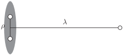
Figure 1: Schematic diagram of the baryons in the diquark-quark picture.

Table 1: The completely antisymmetric states for the diquarks in $\bar{3}_{c}$ Feng:2023txx . $j_{d}$ is the spin of the diquark $(qq^{\prime})$, $s_{d}$ denotes the total spin of two quarks, $l$ represents the orbital angular momentum. $n=n_{r}+1$, $n_{r}$ is the radial quantum number, $n_{r}=0,1,2,\cdots$.

Spin of diquark	Parity	Wave state	Configuration
( $j_{d}$ )	$(j_{d}^{P})$	$(n^{2s_{d}+1}l_{j_{d}})$
$j_{d}=0$	$0^{+}$	$n^{1}s_{0}$	$[qq^{\prime}]^{{\bar{3}_{c}}}_{n^{1}s_{0}}$
	$0^{-}$	$n^{3}p_{0}$	$[qq^{\prime}]^{{\bar{3}_{c}}}_{n^{3}p_{0}}$
$j_{d}=1$	$1^{+}$	$n^{3}s_{1}$, $n^{3}d_{1}$	$\{qq^{\prime}\}^{{\bar{3}_{c}}}_{n^{3}s_{1}}$,  $\{qq^{\prime}\}^{{\bar{3}_{c}}}_{n^{3}d_{1}}$
	$1^{-}$	$n^{1}p_{1}$, $n^{3}p_{1}$	$\{qq^{\prime}\}^{{\bar{3}_{c}}}_{n^{1}p_{1}}$,  $[qq^{\prime}]^{{\bar{3}_{c}}}_{n^{3}p_{1}}$
$j_{d}=2$	$2^{+}$	$n^{1}d_{2}$, $n^{3}d_{2}$	$[qq^{\prime}]^{{\bar{3}_{c}}}_{n^{1}d_{2}}$,  $\{qq^{\prime}\}^{{\bar{3}_{c}}}_{n^{3}d_{2}}$
	$2^{-}$	$n^{3}p_{2}$, $n^{3}f_{2}$	$[qq^{\prime}]^{{\bar{3}_{c}}}_{n^{3}p_{2}}$,  $[qq^{\prime}]^{{\bar{3}_{c}}}_{n^{3}f_{2}}$
$\cdots$	$\cdots$	$\cdots$	$\cdots$

In the diquark picture, the state of a baryon is denoted as

$$\left((qq^{\prime})_{n^{2s_{d}+1}l_{j_{d}}}{{q^{\prime\prime}}}\right)_{N^{2j+1}L_{J}},$$ (1)

where the superscripts $\bar{3}_{c}$, $3_{c}$ and $1_{c}$ are omitted. The diquark $(qq^{\prime})$ is $\{qq^{\prime}\}$ or $[qq^{\prime}]$. $\{qq^{\prime}\}$ and $[qq^{\prime}]$ indicate the permutation symmetric and antisymmetric flavor wave functions, respectively. The completely antisymmetric states for the diquarks in $\bar{3}_{c}$ are listed in Table 1. $N=N_{r}+1$, where $N_{r}=0,\,1,\,\cdots$. $n=n_{r}+1$, where $n_{r}=0,\,1,\,\cdots$. $N_{r}$ and $n_{r}$ are the radial quantum numbers of the baryon and diquark, respectively. $\vec{J}=\vec{L}+\vec{j}$, $\vec{j}=\vec{j}_{d}+\vec{s}_{{q^{\prime\prime}}}$, $\vec{j}_{d}=\vec{s}_{d}+\vec{l}$. $\vec{J}$, $\vec{j}_{d}$ and $\vec{s}_{{q^{\prime\prime}}}$ are the spins of baryon, diquark and quark $q^{\prime\prime}$, respectively. $\vec{j}$ is the summed spin of diquark and quark in the baryon. $L$ and $l$ are the orbital quantum numbers of baryon and diquark, respectively. $\vec{s}_{d}$ is the summed spin of quarks in the diquark.

II.2 Spinless Salpeter equation

The spinless Salpeter equation Godfrey:1985xj ; Ferretti:2019zyh ; Bedolla:2019zwg ; Durand:1981my ; Durand:1983bg ; Lichtenberg:1982jp ; Jacobs:1986gv reads as

$$M\Psi_{d,b}({{\bf r}})=\left(\omega_{1}+\omega_{2}\right)\Psi_{d,b}({{\bf r}})+V_{d,b}\Psi_{d,b}({{\bf r}}),$$ (2)

where $M$ is the bound state mass (diquark or baryon). $\Psi_{d,b}({{\bf r}})$ are the diquark wave function and the baryon wave function, respectively. $V_{d,b}$ denotes the diquark potential and the baryon potential, respectively (see Eq. (4)). $\omega_{1}$ is the relativistic energy of constituent $1$ (quark or diquark), and $\omega_{2}$ is of constituent $2$ (quark),

$$\omega_{i}=\sqrt{m_{i}^{2}+{\bf p}^{2}}=\sqrt{m_{i}^{2}-\Delta}\;\;(i=1,2).$$ (3)

$m_{1}$ and $m_{2}$ are the effective masses of constituent $1$ and $2$, respectively.

When using diquark in multiquark systems, the interactions between quark and quark, diquark and quark, and diquark and diquark are needed. In Ref. Faustov:2021hjs , these interactions are constructed with the help of the off-mass-shell scattering amplitude, which is projected onto the positive energy states. The interactions can also be established by expanding the interactions of the quark-antiquark system to the quark-quark system, and then to the diquark-antidiquark systems or the diquark-quark systems Lundhammar:2020xvw . Furthermore, the effect of the finite size of diquark is treated differently. In Refs. Faustov:2021hjs , the size of diquark is taken into account through corresponding form factors. At times, diquark is taken as being pointlike Ferretti:2019zyh ; Lundhammar:2020xvw ; we use this approximation in the present work.

Following Refs. Ferretti:2019zyh ; Bedolla:2019zwg ; Ferretti:2011zz ; Eichten:1974af ; Chen:2023web ; Chen:2023djq , we employ the potential

$$V_{d,b} =-\frac{3}{4}\left[V_{c}+{\sigma}r+C\right]\left({\bf{F}_{i}}\cdot{\bf{F}_{j}}\right)_{d,b},$$ (4)

where $V_{c}\propto{1/r}$ is a color Coulomb potential or a Coulomb-like potential due to one-gluon-exchange. $\sigma$ is the string tension. $C$ is a fundamental parameter Gromes:1981cb ; Lucha:1991vn . The part in the bracket is the Cornell potential Eichten:1974af . ${\bf{F}_{i}}\cdot{\bf{F}_{j}}$ is the color-Casimir,

$$\langle{(\bf{F}_{i}}\cdot{\bf{F}_{j}})_{d}\rangle=-\frac{2}{3},\quad\langle{(\bf{F}_{i}}\cdot{\bf{F}_{j}})_{b}\rangle=-\frac{4}{3}.$$ (5)

II.3 Regge trajectory relations

For the heavy-heavy systems, $m_{1},m_{2}{\gg}{{|\bf p|}}$, Eq. (2) reduces to

$$M\Psi_{d,t}({{\bf r}}) = \left[(m_{1}+m_{2})+\frac{{{\bf p}}^{2}}{2\mu}\right]\Psi_{d,t}({{\bf r}})$$ (6)

$$+V_{d,t}\Psi_{d,t}({{\bf r}}),$$

where

$$\mu=m_{1}m_{2}/(m_{1}+m_{2}).$$ (7)

By employing the Bohr-Sommerfeld quantization approach Brau:2000st and using Eqs. (4) and (6), we obtain the parameterized relation Chen:2022flh ; Chen:2021kfw

$$M=m_{R}+\beta_{x}(x+c_{0x})^{2/3}\;(x=l,\,n_{r},\,L,\,N_{r})$$ (8)

with

$$m_{R}=m_{1}+m_{2}+C^{\prime},$$ (9)

where

$$C^{\prime}=\left\{\begin{array}[]{cc}C/2,&\text{diquarks},\\ C,&\text{baryons}.\end{array}\right.$$ (10)

$$\sigma^{\prime}=\left\{\begin{array}[]{cc}\sigma/2,&\text{diquarks},\\ \sigma,&\text{baryons}.\end{array}\right.$$ (11)

$\beta_{x}$ reads

$$\beta_{x}=c_{fx}c_{x}c_{c}.$$ (12)

$c_{c}$ and $c_{x}$ are

$$c_{c}=\left(\frac{\sigma^{\prime 2}}{\mu}\right)^{1/3},\;c_{l}=\frac{3}{2},\;c_{n_{r}}=\frac{\left(3\pi\right)^{2/3}}{2}.$$ (13)

Both $c_{fl}$ and $c_{fn_{r}}$ are equal theoretically to one and are fitted in practice. In Eq. (8), $m_{1}$, $m_{2}$, $c_{x}$ and $\sigma$ are universal. $c_{0x}$ are determined by fit. $c_{fl}$ and $c_{fn_{r}}$ are theoretically equal to one but are fitted in practice.

For the heavy-light systems ($m_{1}\to\infty$ and $m_{2}\to 0$), Eq. (2) simplifies to

$$M\Psi_{d,t}({{\bf r}})=\left[m_{1}+{{|\bf p|}}+V_{d,t}\right]\Psi_{d,t}({{\bf r}}).$$ (14)

By employing the Bohr-Sommerfeld quantization approach Brau:2000st , the parameterized formula can be written as Chen:2022flh ; Chen:2021kfw

$$M=m_{R}+\beta_{x}\sqrt{x+c_{0x}}\;(x=l,\,n_{r},\,L,\,N_{r}).$$ (15)

The parameters in Eq. (15) read as

$$c_{c}=\sqrt{\sigma^{\prime}},\;c_{l}=2,\;c_{n_{r}}=\sqrt{2\pi}.$$ (16)

For the heavy-light systems, the common choice of $m_{R}$ is Selem:2006nd ; Chen:2021kfw ; Veseli:1996gy

$$m_{R}=m_{1}.$$ (17)

Eq. (15) with (17) is obtained in the limit $m_{1}\to\infty$ and $m_{2}\to 0$. There are different ways to include the light constituent’s mass Selem:2006nd ; Nielsen:2018uyn ; Sonnenschein:2018fph ; MartinContreras:2020cyg ; Chen:2023cws ; Chen:2023ngj ; Chen:2022flh ; Chen:2014nyo ; Afonin:2014nya ; Sergeenko:1994ck . Two modified formulas are proposed in Ref. Chen:2023cws , which can universally describe both the heavy-light mesons and the heavy-light diquarks. One is Eq. (15) with (9). Another reads

$$M=m_{R}+\sqrt{\beta_{x}^{2}(x+c_{0x})+\kappa_{x}m^{3/2}_{2}(x+c_{0x})^{1/4}}$$ (18)

if $m_{2}{\ll}M$, where

$$m_{R}=m_{1}+C^{\prime},\quad\kappa_{x}=\frac{4}{3}\sqrt{{\pi}\beta_{x}},$$ (19)

where $\beta_{x}$ is in (24). Eq. (15) with (9) is an extension of Afonin:2014nya

$$M=m_{1}+m_{2}+\sqrt{a(n_{r}+{\alpha}l+b)}$$ (20)

and the formula Chen:2022flh

$$(M-m_{1}-m_{2}-C)^{2}=\alpha_{x}(x+c_{0})^{\gamma}$$ (21)

while (18) with (19) is based on the results in Selem:2006nd ; Sonnenschein:2018fph . Although they give different behavior of $m_{2}$, Eq. (15) with (9) and Eq. (18) with (19) produce consistent results for $l,\,n_{r}<10$ and have the same behavior $M{\sim}x^{1/2}$ Chen:2023cws .

For the light systems ($m_{1},\,m_{2}\to 0$), Eq. (2) simplifies to

$$M\Psi_{d,t}({{\bf r}})=\left[2{{|\bf p|}}+V_{d,t}\right]\Psi_{d,t}({{\bf r}}).$$ (22)

By employing the Bohr-Sommerfeld quantization approach Brau:2000st , the parameterized formula can be written as Chen:2022flh ; Chen:2021kfw

$$M=\beta_{x}\sqrt{x+c_{0x}}\;(x=l,\,n_{r},\,L,\,N_{r}).$$ (23)

For the light systems, the parameters read as

$$c_{c}=\sqrt{\sigma^{\prime}},\;c_{l}=2\sqrt{2},\;c_{n_{r}}=2\sqrt{\pi}.$$ (24)

According to the results in Refs. Selem:2006nd ; Sonnenschein:2018fph , similar to Eq. (18) proposed in Chen:2023cws , we suggest

$$M=C^{\prime}+\sqrt{\beta_{x}^{2}(x+c_{0x})+\kappa_{x}\left(m_{1}^{3/2}+m_{2}^{3/2}\right)(x+c_{0x})^{1/4}}.$$ (25)

Based on Eq. (20) Afonin:2014nya , we obtain a modified Regge trajectory relation for the light-light systems in Ref. Chen:2023ngj

$$M=m_{R}+\beta_{x}\sqrt{x+c_{0x}},$$ (26)

where

$$c_{c}=\sqrt{\sigma^{\prime}},\;c_{l}=2\sqrt{2},\;c_{n_{r}}=2\sqrt{\pi}.$$ (27)

$m_{R}$ is in Eq. (9).

Table 2: The coefficients for the heavy-heavy systems (HHS), the heavy-light systems (HLS), and the light-light systems (LLS).

	HHS	HLS	LLS
$\nu$	$2/3$	$1/2$	$1/2$
$c_{c}$	$\left({\sigma^{\prime 2}}/{\mu}\right)^{1/3}$	$\sqrt{\sigma^{\prime}}$	$\sqrt{\sigma^{\prime}}$
$c_{l,\,L}$	$3/2$	$2$	$2\sqrt{2}$
$c_{n_{r},\,N_{r}}$	${\left(3\pi\right)^{2/3}}/{2}$	$\sqrt{2\pi}$	$2\sqrt{\pi}$

When Eq. (15) with (9) is employed to discuss the heavy-light systems, and Eq. (26) with (9) is used to discuss the light systems, summarising Eqs. (8), (15) with (9) and (26) with (9), we have a general form of the Regge trajectories Chen:2022flh ; Xie:2024dfe

$$M= m_{R}+\beta_{x}(x+c_{0x})^{\nu}\,\,(x=l,\,n_{r},\,L,\,N_{r}),$$

$$m_{R}= m_{1}+m_{2}+C^{\prime},\quad\beta_{x}=c_{fx}c_{x}c_{c},$$ (28)

where ${\nu}$, $c_{x}$ and $c_{c}$ are listed in Table 2. $c_{fx}$ are theoretically equal to one and are fitted in practice. $c_{0x}$ vary with different Regge trajectories. Eq. (II.3) can be employed to discuss various systems including the heavy-heavy systems, the heavy-light systems, and the light-light systems: diquarks, mesons, baryons, and tetraquarks Chen:2023djq ; Chen:2023ngj ; Chen:2023web .

We notice that the general form (II.3) remains open and is provisional. Because there are different methods to include the masses of the light constituents. More theoretical and experimental data are needed. In addition, the parameter values are universal for both the heavy-heavy systems and the heavy-light systems Chen:2023cws ; Feng:2023txx . However, the parameter values change for the light systems Chen:2023ngj to obtain agreeable results.

II.4 Behaviors of the Regge trajectories for baryons

As an example, we consider the baryon $(qq^{\prime}){{q^{\prime\prime}}}$, in which the light diquark $(qq^{\prime})$ is composed of two light quarks and ${{q^{\prime\prime}}}$ is also light. When discussing the Regge trajectories of the light diquarks, Eq. (25) gives the same behavior as Eq. (26) with (9),

$$M_{\rho}{\sim}x_{\rho}^{1/2},$$ (29)

where $M_{\rho}$ is the diquark mass. Generally speaking, the diquark Regge trajectories are not the same as the $\rho$-trajectories of baryons. For a light diquark composed of two light quarks, the behavior of the diquark Regge trajectory is definite (see Eq. (29)) if the masses of light quarks are not considered. However, it is indefinite when discussing the $\rho$- and $\lambda$-trajectories of baryons composed of the light diquark and/or the light quark. If the diquark $(qq^{\prime})$ is regarded as being light, when Eq. (25) is chosen as the $\lambda$-trajectory relation, it will give $M{\sim}M_{\rho}^{3/2}$ while Eq. (26) with (9) gives $M{\sim}M_{\rho}$ due to different ways to include the light constituent’s mass $M_{\rho}$ [corresponding to $m_{1,2}$ in Eq. (25) and (26) with (9).]. They give two different behaviors of the $\rho$-trajectories. Using Eq. (29), Eq. (25) gives $M{\sim}x_{\rho}^{3/4}$ while Eq. (26) with (9) gives $M{\sim}x_{\rho}^{1/2}$. When discussing the $\rho$-trajectories, highly excited diquark will be involved. The first radially and orbitally excited $(ud)$ are about $1.3$ GeV. The masses of the $1^{1}p_{1}$ states of $(us)$ and $(ss)$ are much heavier, $1.46$ GeV and $1.65$ GeV Chen:2023ngj , respectively. They approximate or even exceed the mass of the charm quark. Therefore, the light diquark composed of two light quarks can be regarded as being heavy when discussing the $\rho$-trajectories of baryons. Then, Eq. (15) with (9) or Eq. (18) with (19) can be chosen as the ${\lambda}$-trajectory formula. They will give the same $\rho$-trajectory behavior, $M{\sim}M_{\rho}$. Using Eq. (29), we get $M{\sim}x_{\rho}^{1/2}$.

Table 3: Behaviors of two series of Regge trajectories for different baryons in the diquark picture. $Q=c,\,b$ and $q=u,\,d,\,s$. $M$ is the mass of the baryons. $x_{\lambda}=L,\,N_{r}$ are the angular momentum quantum number and the radial quantum number for the $\lambda$ mode. $x_{\rho}=l,\,n_{r}$ are for the $\rho$ mode. ${\,{\boldsymbol{?}}}$ denotes the indefinite result.

		Traj. behavior $M{\sim}x^{\nu}$		Traj. behavior $M^{2}{\sim}x^{\nu^{\prime}}$
		$\rho$-mode	$\lambda$-mode	$\rho$-mode	$\lambda$-mode
1	$(qq^{\prime})q^{\prime\prime}$	$x_{\rho}^{1/2}$, $x_{\rho}^{3/4}$${\,{\boldsymbol{?}}}$	$x_{\lambda}^{1/2}$	$x_{\rho}$, $x_{\rho}^{3/4}$${\,{\boldsymbol{?}}}$	$x_{\lambda}$, $x_{\lambda}^{1/2}$${\,{\boldsymbol{?}}}$
2	$(qq^{\prime})Q$	$x_{\rho}^{1/2}$, $x_{\rho}^{3/4}$${\,{\boldsymbol{?}}}$	$x_{\lambda}^{1/2}$, $x_{\lambda}^{2/3}$${\,{\boldsymbol{?}}}$	$x_{\rho}^{1/2}$, $x_{\rho}^{3/4}$${\,{\boldsymbol{?}}}$	$x_{\lambda}^{1/2}$, $x_{\lambda}^{2/3}$${\,{\boldsymbol{?}}}$
3	$(Qq)q^{\prime}$	$x_{\rho}^{1/2}$	$x_{\lambda}^{1/2}$	$x_{\rho}^{1/2}$	$x_{\lambda}^{1/2}$
4	$(Qq^{\prime})Q^{\prime}$	$x_{\rho}^{1/2}$	$x_{\lambda}^{2/3}$	$x_{\rho}^{1/2}$	$x_{\lambda}^{2/3}$
5	$(QQ^{\prime})q$	$x_{\rho}^{2/3}$	$x_{\lambda}^{1/2}$	$x_{\rho}^{2/3}$	$x_{\lambda}^{1/2}$
6	$(QQ^{\prime})Q^{\prime\prime}$	$x_{\rho}^{2/3}$	$x_{\lambda}^{2/3}$	$x_{\rho}^{2/3}$	$x_{\lambda}^{2/3}$

If the light diquark is regarded as being light, $\lambda$-trajectories behave as $M{\sim}x^{1/2}_{\lambda}$ no matter if Eq. (25) or Eq. (26) with (9) is chosen as the $\lambda$-trajectory formula. If the light diquark is regarded as being heavy, $\lambda$-trajectories also behave as $M{\sim}x_{\lambda}^{1/2}$ according to Eq. (15) with (9) or Eq. (18) with (19). Therefore, the behavior of the $\lambda$-trajectories is definite whether the light diquark is regarded as being light or being heavy.

As in the preceding discussions, when the diquark in a baryon is composed of two light quarks, discussing the Regge trajectories will be confronted with two problems. One is when the light diquark can be regarded as being heavy, which will affect not only the behaviors of the ${\lambda}$-trajectories but also those of the $\rho$-trajectories. Another is how to introduce the mass of the light constituent if the diquark is light, which will effect the behavior of the $\rho$-trajectories. These two problems remain open; thus, the behaviors of the Regge trajectories of the baryons containing the light diquark remain indefinite, see Table 3.

When the diquark is doubly heavy or heavy-light, it is clear how to introduce its large mass, and the way of introducing the light mass does not affect the Regge trajectory behaviors (see Eqs. (8) with (9) and Eq. (15) with (9) or Eq. (18) with (19)). The Regge trajectory formulas can be written explicitly, and then the behaviors of the $\lambda$-trajectory and the $\rho$-trajectory are definite. For example, the Regge trajectory for the baryons composed of one doubly heavy diquark and one heavy quark can be written explicitly as Eq. (II.5) with (II.5). Other types of baryons can be discussed in a similar manner. The Regge trajectory behaviors of different types of baryons are listed in Table 3.

The behaviors of the Regge trajectories discussed are for the linearly confining potential $V_{c}{\sim}r$, and they vary with different confining potentials. Moreover, the results in Table 3 are obtained without considering various mixings. When the mixings are considered, the behaviors of the Regge trajectories will become complex.

In Ref. Chen:2023web , we suggest that all Regge trajectories for the diquarks, mesons, baryons, and tetraquarks are concave downwards in the $(M^{2},\,x)$ $(x=L,\,N_{r})$ planes. For the light systems, the Regge trajectories are also concave when considering the masses of the light constituents. The trajectories for baryons and tetraquarks discussed in Refs. Chen:2023web ; Chen:2023djq in fact are the $\lambda$-trajectories. We can see from Table 3 that both the $\lambda$-trajectories and the $\rho$-trajectories of various baryons are all concave downwards in the $(M^{2},\,x)$ $(x=l,\,n_{r},\,L,\,N_{r})$ planes. For the light systems, the trajectories approximate linearity as the masses are neglected and become concave when the masses are considered.

II.5 Regge trajectory relations for the triply heavy baryons

A triply heavy baryon consists of one doubly heavy diquark $(QQ^{\prime})$ and one heavy quark $Q^{\prime\prime}$. According to Eq. (II.3), we have the Regge trajectory relations for the triply heavy baryons

$$M =m_{R{\lambda}}+\beta_{x_{\lambda}}(x_{\lambda}+c_{0x_{\lambda}})^{2/3}\;(x_{\lambda}=L,\,N_{r}),$$

$$M_{\rho} =m_{R\rho}+\beta_{x_{\rho}}(x_{\rho}+c_{0x_{\rho}})^{2/3}\;(x_{\rho}=l,\,n_{r}),$$ (30)

where

$$m_{R{\lambda}} =M_{\rho}+m_{Q^{\prime\prime}}+C,$$

$$m_{R\rho} =m_{Q}+m_{Q^{\prime}}+C/2,$$

$$\beta_{L} =\frac{3}{2}\left(\frac{\sigma^{2}}{\mu_{\lambda}}\right)^{1/3}c_{fL},\;\beta_{N_{r}}=\frac{(3\pi)^{2/3}}{2}\left(\frac{\sigma^{2}}{\mu_{\lambda}}\right)^{1/3}c_{fN_{r}},$$

$$\mu_{\lambda} =\frac{M_{\rho}m_{Q^{\prime\prime}}}{M_{\rho}+m_{Q^{\prime\prime}}},\;\mu_{\rho}=\frac{m_{Q}m_{Q^{\prime}}}{m_{Q}+m_{Q^{\prime}}},$$

$$\beta_{l} =\frac{3}{2}\left(\frac{\sigma^{2}}{4\mu_{\rho}}\right)^{1/3}c_{fl},\;\beta_{n_{r}}=\frac{(3\pi)^{2/3}}{2}\left(\frac{\sigma^{2}}{4\mu_{\rho}}\right)^{1/3}c_{fn_{r}}.$$ (31)

In Eq. (II.5), $M$ is the baryon mass, and $M_{\rho}$ is the diquark mass. The second relation in Eq. (II.5) is used to calculate the diquark masses. The first relation in Eq. (II.5) together with other relations in Eq. (II.5) and (II.5) is employed to calculate the baryon mass. It is obvious that there are two series of Regge trajectories for the triply heavy baryons.

III Regge trajectories for $\Omega_{ccb}$ and $\Omega_{cbb}$

In this section, both the $\lambda-$trajectories and the $\rho-$trajectories for the triply heavy bottom-charm baryon are investigated.

III.1 Parameters

The quark masses, the string tension $\sigma$, and the parameter $C$ are from Ref. Faustov:2021qqf . The parameters for the doubly heavy diquarks $(cc)$ and $(bb)$ are from Ref. Feng:2023txx and listed in Table 4. With these parameters determined, the $\rho-$modes and the diquark masses can be discussed (see Eqs. (II.5) and (II.5)). To discuss the $\lambda-$modes excited states, the parameters $c_{fL}$, $c_{fN_{r}}$, $c_{0{L}}$, and $c_{0N_{r}}$ should be determined (see Eqs. (32) and (33)). More detailed discussions are in Xie:2024dfe .

Table 4: The values of parameters Feng:2023txx ; Faustov:2021qqf .

	$m_{c}=1.55\;{{\rm GeV}}$,   $m_{b}=4.88\;{{\rm GeV}}$,
	$\sigma=0.18\;{{\rm GeV}^{2}}$,  $C=-0.3\;{{\rm GeV}}$,
$(cc)$	$c_{fn_{r}}=1.0$,  $c_{fl}=1.17$,
	$c_{0n_{r}}(1^{3}s_{1})=0.205$, $c_{0{l}}(1^{3}s_{1})=0.337$,
$(bb)$	$c_{fn_{r}}=1.0$,  $c_{fl}=1.17$,
	$c_{0n_{r}}(1^{3}s_{1})=0.01$, $c_{0{l}}(1^{3}s_{1})=0.001$.

According to Eq. (II.5), $c_{fx_{\lambda}}$ and $c_{0x_{\lambda}}$ are needed to determine a Regge trajectory as $m_{R_{\lambda}}$ can be calculated by using Eq. (II.5) and parameters in Table 4. Two or more states on the Regge trajectory are needed to obtain $c_{fx_{\lambda}}$ and $c_{0x_{\lambda}}$. Since the experimental data are absent, we choose $c_{fx_{\lambda}}$ and $c_{0x_{\lambda}}$ by fitting these parameters from other systems. In addition, $c_{fx_{\lambda}}$ and $c_{0x_{\lambda}}$ vary with masses of constituents. We obtain the fitted parameter relations in Ref. Xie:2024dfe

$$c_{fL}= 1.116+0.013\mu_{\lambda},\;c_{0L}=0.540-0.141\mu_{\lambda},$$ (32)

$$c_{fN_{r}}= 1.008+0.008\mu_{\lambda},\;c_{0N_{r}}=0.334-0.087\mu_{\lambda},$$ (33)

where $\mu_{\lambda}$ is the reduced masses, see Eq. (II.5). As more experimental data or more theoretical data become available, the fitted formulas will be refined.

III.2 $\lambda-$ and $\rho-$trajectories

Table 5: The spin-averaged masses of the $\lambda$-excited states of $\Omega_{ccb}$ and $\Omega_{cbb}$ (in ${{\rm GeV}}$). The notation in Eq. (1) is rewritten as $|n^{2s_{d}+1}l_{j_{d}},N^{2j+1}L_{J}\rangle$. And $|n^{2s_{d}+1}l_{j_{d}},NL\rangle$ denotes the spin-averaged states. Eqs. (II.5), (32) and (33) are used.

$|n^{2s_{d}+1}l_{j_{d}},NL\rangle$	$(cc)b$	$c(bb)$
$|1^{3}s_{1},1S\rangle$	7.88	11.11
$|1^{3}s_{1},2S\rangle$	8.35	11.63
$|1^{3}s_{1},3S\rangle$	8.68	11.99
$|1^{3}s_{1},4S\rangle$	8.97	12.31
$|1^{3}s_{1},5S\rangle$	9.22	12.59
$|1^{3}s_{1},1S\rangle$	7.88	11.12
$|1^{3}s_{1},1P\rangle$	8.22	11.48
$|1^{3}s_{1},1D\rangle$	8.46	11.75
$|1^{3}s_{1},1F\rangle$	8.67	11.98
$|1^{3}s_{1},1G\rangle$	8.86	12.19
$|1^{3}s_{1},1H\rangle$	9.03	12.38

Table 6: Same as Table 5 except for the $\rho$-excited states. $\times$ denotes the nonexist states.

$|n^{2s_{d}+1}l_{j_{d}},NL\rangle$	$(cc)b$	$c(bb)$
$|1^{3}s_{1},1S\rangle$	7.88	11.11
$|2^{3}s_{1},1S\rangle$	8.25	11.43
$|3^{3}s_{1},1S\rangle$	8.52	11.63
$|4^{3}s_{1},1S\rangle$	8.74	11.79
$|5^{3}s_{1},1S\rangle$	8.95	11.94
$|1^{3}s_{1},1S\rangle$	7.89	11.10
$|1^{3}p_{2},1S\rangle$$(\times)$	8.17	11.36
$|1^{3}d_{3},1S\rangle$	8.37	11.51
$|1^{3}f_{4},1S\rangle$$(\times)$	8.55	11.64
$|1^{3}g_{5},1S\rangle$	8.70	11.76
$|1^{3}h_{6},1S\rangle$$(\times)$	8.85	11.86

Table 7: Comparison of theoretical predictions for the spin averaged masses of the triply heavy bottom-charm baryons baryons (in GeV).

Baryon	$|n^{2s_{d}+1}l_{j_{d}},NL\rangle$	Our	Ref. Faustov:2021qqf	Ref. Silvestre-Brac:1996myf	Ref. Yang:2019lsg	Ref. Roberts:2007ni
$\Omega_{ccb}$	$|1^{3}s_{1},1S\rangle$	7.88	7.99	8.04	8.02	8.26
	$|1^{3}s_{1},2S\rangle$	8.35	8.41	8.46	8.46
	$|1^{3}s_{1},1P\rangle$	8.22	8.26	8.32	8.31	8.42
	$|2^{3}s_{1},1S\rangle$	8.25	8.36
$\Omega_{cbb}$	$|1^{3}s_{1},1S\rangle$	11.11	11.21	11.24	11.21	11.55
	$|1^{3}s_{1},2S\rangle$	11.63	11.70	11.64	11.62
	$|1^{3}s_{1},1P\rangle$	11.48	11.53	11.55	11.51	11.74
	$|2^{3}s_{1},1S\rangle$	11.43	11.51

Figure 2: The $\lambda$-trajectories for the triply heavy bottom-charm baryons. Circles represent the predicted data and the black lines are the $\lambda$-trajectories, see Eq. (II.5). Data are listed in Table 5.

Figure 3: The $\rho$-trajectories for the triply heavy bottom-charm baryons. Circles represent the predicted data and the black lines are the $\rho$-trajectories, see Eq. (II.5). Data are listed in Table 6.

By using Eqs. (II.5), (32) and (33), along with the parameters in Table 4, the spin-averaged masses of the $\lambda$-excitations and $\rho$-excitations are estimated (see Tables 5 and 6). The obtained results are in agreement with other theoretical predictions, see Table 7. The $\lambda$-trajectories and $\rho$-trajectories are shown in Figs. 2 and 3.

There are two series of masses: one is for the $\lambda$-excited states and the other is for the $\rho$-excited states. There is no degeneracy in masses, see Tables 5 and 6. For an excited state, the mass of the $\lambda$-mode will be larger than that of the $\rho$-mode. There exist mixing between $\lambda$-excitations and $\rho$-excitations or between $\lambda$-excitations themselves, for example, $3p1S-1s2P$ with $J^{P}=1/2^{-}$ and $3/2^{-}$ Gershtein:2000nx . In this work, different mixings are not considered.

Both the diquarks ($(bb)$ and $(cc)$) and the quarks ($b$ and $c$) are heavy; therefore, the case of the triply heavy bottom-charm baryons is simple, and the Regge trajectory relations can be written explicitly, see (II.5). From Eq. (II.5), we can see easily that the $\lambda$-trajectories and $\rho$-trajectories have the same behaviors, $M{\sim}x^{2/3}_{\lambda}$ and $M{\sim}x^{2/3}_{\rho}$.

The curvature of the Regge trajectories holds significant importance Chen:2018bbr . In potential models, the curvature is related to the dynamic equation and the confining potential. In this work, we show that for the triply heavy bottom-charm baryon, not only the $\lambda$-trajectories but also the $\rho$-trajectories are concave in the $(M^{2},\,x)$ planes, see Eq. (II.5).

IV Conclusions

By employing the diquark Regge trajectory relation, we present explicitly the Regge trajectory relations for the triply heavy bottom-charm baryons, which can investigate both the $\lambda$-mode excited states and the $\rho$-mode excited states. We estimate the masses of the $\lambda$-excited states and the $\rho$-excited states. The results are in agreement with other theoretical predictions.

Both the $\lambda$-trajectories and the $\rho$-trajectories are discussed. The $\rho$-trajectories behave as $M{\sim}x_{\rho}^{2/3}$ because the $\rho$-mode excitations are in the doubly heavy diquarks ($(bb)$ or $(cc)$), which are the heavy-heavy systems. Similarly, the $\lambda$-trajectories behave as $M{\sim}x_{\lambda}^{2/3}$ because the $\lambda$-mode excitations occur between the doubly heavy diquark and the heavy quark, with the diquark ($(cc)$ or $(bb)$) and quark ($b$ or $c$) forming a heavy-heavy system.

Moreover, the behaviors of the $\lambda$- and $\rho$-trajectories for various baryons are discussed. It is shown that both the $\lambda$-trajectories and the $\rho$-trajectories for baryons are concave downwards in the $(M^{2},\,x)$ plane. The Regge trajectories for the light baryons approximate linearity and become concave as the masses of the light constituents are considered.

Appendix A States of baryons

The states of baryons in the diquark picture are listed in Table 8.

Table 8: The states of baryons in the diquark picture. The notation is explained in II.1. Here, $q$, ${q^{\prime}}$ and ${q^{\prime\prime}}$ represent both the light quarks and the heavy quarks.

$J^{P}$	$(L,l)$	Configuration
$\frac{1}{2}^{+}$	$(0,0)$	$\left({{[qq^{\prime}]}}_{n^{1}s_{0}}{{q^{\prime\prime}}}\right)_{N^{2}S_{1/2}}$,  $\left({\{qq^{\prime}\}}_{n^{3}s_{1}}{{q^{\prime\prime}}}\right)_{N^{2}S_{1/2}}$,
	$(1,1)$	$\left({\{qq^{\prime}\}}_{n^{1}p_{1}}{{q^{\prime\prime}}}\right)_{N^{2}P_{1/2}}$,  $\left({\{qq^{\prime}\}}_{n^{1}p_{1}}{{q^{\prime\prime}}}\right)_{N^{4}P_{1/2}}$,  $\left({{[qq^{\prime}]}}_{n^{3}p_{0}}{{q^{\prime\prime}}}\right)_{N^{2}P_{1/2}}$,  $\left({{[qq^{\prime}]}}_{n^{3}p_{1}}{{q^{\prime\prime}}}\right)_{N^{2}P_{1/2}}$,
		$\left({{[qq^{\prime}]}}_{n^{3}p_{1}}{{q^{\prime\prime}}}\right)_{N^{4}P_{1/2}}$,  $\left({{[qq^{\prime}]}}_{n^{3}p_{2}}{{q^{\prime\prime}}}\right)_{N^{4}P_{1/2}}$
	$\cdots$	$\cdots$
$\frac{1}{2}^{-}$	$(1,0)$	$\left({{[qq^{\prime}]}}_{n^{1}s_{0}}{{q^{\prime\prime}}}\right)_{N^{2}P_{1/2}}$,  $\left({\{qq^{\prime}\}}_{n^{3}s_{1}}{{q^{\prime\prime}}}\right)_{N^{2}P_{1/2}}$,  $\left({\{qq^{\prime}\}}_{n^{3}s_{1}}{{q^{\prime\prime}}}\right)_{N^{4}P_{1/2}}$,
	$(0,1)$	$\left({\{qq^{\prime}\}}_{n^{1}p_{1}}{{q^{\prime\prime}}}\right)_{N^{2}S_{1/2}}$,  $\left({{[qq^{\prime}]}}_{n^{3}p_{0}}{{q^{\prime\prime}}}\right)_{N^{2}S_{1/2}}$,  $\left({{[qq^{\prime}]}}_{n^{3}p_{1}}{{q^{\prime\prime}}}\right)_{N^{2}S_{1/2}}$,
	$\cdots$	$\cdots$
$\frac{3}{2}^{+}$	$(0,0)$	$\left({\{qq^{\prime}\}}_{n^{3}s_{1}}{{q^{\prime\prime}}}\right)_{N^{4}S_{3/2}}$,
	$(1,1)$	$\left({\{qq^{\prime}\}}_{n^{1}p_{1}}{{q^{\prime\prime}}}\right)_{N^{2}P_{3/2}}$,  $\left({\{qq^{\prime}\}}_{n^{1}p_{1}}{{q^{\prime\prime}}}\right)_{N^{4}P_{3/2}}$,  $\left({{[qq^{\prime}]}}_{n^{3}p_{0}}{{q^{\prime\prime}}}\right)_{N^{2}P_{3/2}}$,  $\left({{[qq^{\prime}]}}_{n^{3}p_{1}}{{q^{\prime\prime}}}\right)_{N^{2}P_{3/2}}$,
		$\left({{[qq^{\prime}]}}_{n^{3}p_{1}}{{q^{\prime\prime}}}\right)_{N^{4}P_{3/2}}$,  $\left({{[qq^{\prime}]}}_{n^{3}p_{2}}{{q^{\prime\prime}}}\right)_{N^{4}P_{3/2}}$,  $\left({{[qq^{\prime}]}}_{n^{3}p_{2}}{{q^{\prime\prime}}}\right)_{N^{6}P_{3/2}}$,
	$\cdots$	$\cdots$
$\frac{3}{2}^{-}$	$(1,0)$	$\left({{[qq^{\prime}]}}_{n^{1}s_{0}}{{q^{\prime\prime}}}\right)_{N^{2}P_{3/2}}$,  $\left({\{qq^{\prime}\}}_{n^{3}s_{1}}{{q^{\prime\prime}}}\right)_{N^{2}P_{3/2}}$,  $\left({\{qq^{\prime}\}}_{n^{3}s_{1}}{{q^{\prime\prime}}}\right)_{N^{4}P_{3/2}}$,
	$(0,1)$	$\left({\{qq^{\prime}\}}_{n^{1}p_{1}}{{q^{\prime\prime}}}\right)_{N^{4}S_{3/2}}$,  $\left({{[qq^{\prime}]}}_{n^{3}p_{1}}{{q^{\prime\prime}}}\right)_{N^{4}S_{3/2}}$,  $\left({{[qq^{\prime}]}}_{n^{3}p_{2}}{{q^{\prime\prime}}}\right)_{N^{4}S_{3/2}}$
	$\cdots$	$\cdots$

References

• (1) N. Mathur, M. Padmanath and S. Mondal, Phys. Rev. Lett. 121, no.20, 202002 (2018) doi:10.1103/PhysRevLett.121.202002 [arXiv:1806.04151 [hep-lat]].
• (2) K. Serafin, M. Gómez-Rocha, J. More and S. D. Głazek, Eur. Phys. J. C 78, no.11, 964 (2018) doi:10.1140/epjc/s10052-018-6436-2 [arXiv:1805.03436 [hep-ph]].
• (3) R. N. Faustov and V. O. Galkin, Phys. Rev. D 105, no.1, 014013 (2022) doi:10.1103/PhysRevD.105.014013 [arXiv:2111.07702 [hep-ph]].
• (4) B. Silvestre-Brac, Few Body Syst. 20, 1-25 (1996) doi:10.1007/s006010050028
• (5) W. Roberts and M. Pervin, Int. J. Mod. Phys. A 23, 2817-2860 (2008) doi:10.1142/S0217751X08041219 [arXiv:0711.2492 [nucl-th]].
• (6) N. M. de Arenaza, J. J. Gálvez-Viruet and F. J. Llanes-Estrada, [arXiv:2407.07232 [nucl-th]].
• (7) G. Yang, J. Ping, P. G. Ortega and J. Segovia, Chin. Phys. C 44, no.2, 023102 (2020) doi:10.1088/1674-1137/44/2/023102 [arXiv:1904.10166 [hep-ph]].
• (8) P. Hasenfratz, R. R. Horgan, J. Kuti and J. M. Richard, Phys. Lett. B 94, 401-404 (1980) doi:10.1016/0370-2693(80)90906-5
• (9) J. R. Zhang and M. Q. Huang, Phys. Lett. B 674, 28-35 (2009) doi:10.1016/j.physletb.2009.02.056 [arXiv:0902.3297 [hep-ph]].
• (10) Z. R. Najjar, K. Azizi and H. R. Moshfegh, Eur. Phys. J. C 84, no.6, 612 (2024) doi:10.1140/epjc/s10052-024-12960-x [arXiv:2402.14348 [hep-ph]].
• (11) Z. G. Wang, Commun. Theor. Phys. 58, 723-731 (2012) doi:10.1088/0253-6102/58/5/17 [arXiv:1112.2274 [hep-ph]].
• (12) A. P. Martynenko, Phys. Lett. B 663, 317-321 (2008) doi:10.1016/j.physletb.2008.04.030 [arXiv:0708.2033 [hep-ph]].
• (13) Y. Jia, JHEP 10, 073 (2006) doi:10.1088/1126-6708/2006/10/073 [arXiv:hep-ph/0607290 [hep-ph]].
• (14) P. L. Yin, C. Chen, G. Krein, C. D. Roberts, J. Segovia and S. S. Xu, Phys. Rev. D 100, no.3, 034008 (2019) doi:10.1103/PhysRevD.100.034008 [arXiv:1903.00160 [nucl-th]].
• (15) S. Ishida, M. Ishida and K. Yamada, Prog. Theor. Phys. 91, 775-800 (1994) doi:10.1143/PTP.91.775
• (16) J. K. Chen, Nucl. Phys. A 1050, 122927 (2024) doi:10.1016/j.nuclphysa.2024.122927 [arXiv:2302.05926 [hep-ph]].
• (17) J. Oudichhya, K. Gandhi and A. k. Rai, Pramana 97, no.4, 151 (2023) doi:10.1007/s12043-023-02630-0 [arXiv:2304.05110 [hep-ph]].
• (18) J. K. Chen, Nucl. Phys. B 983, 115911 (2022) doi:10.1016/j.nuclphysb.2022.115911 [arXiv:2203.02981 [hep-ph]].
• (19) J. K. Chen, X. Feng and J. Q. Xie, JHEP 10, 052 (2023) doi:10.1007/JHEP10(2023)052 [arXiv:2308.02289 [hep-ph]].
• (20) T. J. Burns, F. Piccinini, A. D. Polosa and C. Sabelli, Phys. Rev. D 82, 074003 (2010) doi:10.1103/PhysRevD.82.074003 [arXiv:1008.0018 [hep-ph]].
• (21) J. K. Chen, Eur. Phys. J. A 57, 238 (2021) doi:10.1140/epja/s10050-021-00502-y [arXiv:2102.07993 [hep-ph]].
• (22) J. K. Chen, Eur. Phys. J. C 78, no.8, 648 (2018) doi:10.1140/epjc/s10052-018-6134-0
• (23) J. Q. Xie, H. Song, X. Feng and J. K. Chen, [arXiv:2407.04222 [hep-ph]].
• (24) J. K. Chen, Eur. Phys. J. C 84, no.4, 356 (2024) doi:10.1140/epjc/s10052-024-12706-9 [arXiv:2302.06794 [hep-ph]].
• (25) X. Feng, J. K. Chen and J. Q. Xie, Phys. Rev. D 108, no.3, 034022 (2023) doi:10.1103/PhysRevD.108.034022 [arXiv:2305.15705 [hep-ph]].
• (26) J. K. Chen, J. Q. Xie, X. Feng and H. Song, Eur. Phys. J. C 83, no.12, 1133 (2023) doi:10.1140/epjc/s10052-023-12329-6 [arXiv:2310.05131 [hep-ph]].
• (27) Jia-Qi Xie, He Song and Jiao-Kai Chen, in progress.
• (28) M. A. Bedolla, J. Ferretti, C. D. Roberts and E. Santopinto, Eur. Phys. J. C 80, no.11, 1004 (2020) doi:10.1140/epjc/s10052-020-08579-3 [arXiv:1911.00960 [hep-ph]].
• (29) J. Ferretti, Few Body Syst. 60, no.1, 17 (2019) doi:10.1007/s00601-019-1483-2
• (30) S. Godfrey and N. Isgur, Phys. Rev. D 32, 189-231 (1985) doi:10.1103/PhysRevD.32.189
• (31) B. Durand and L. Durand, Phys. Rev. D 25, 2312 (1982) doi:10.1103/PhysRevD.25.2312
• (32) B. Durand and L. Durand, Phys. Rev. D 30, 1904 (1984) doi:10.1103/PhysRevD.30.1904
• (33) D. B. Lichtenberg, W. Namgung, E. Predazzi and J. G. Wills, Phys. Rev. Lett. 48, 1653 (1982) doi:10.1103/PhysRevLett.48.1653
• (34) S. Jacobs, M. G. Olsson and C. Suchyta, III, Phys. Rev. D 33, 3338 (1986) [erratum: Phys. Rev. D 34, 3536 (1986)] doi:10.1103/PhysRevD.33.3338
• (35) R. N. Faustov, V. O. Galkin and E. M. Savchenko, Universe 7, no.4, 94 (2021) doi:10.3390/universe7040094 [arXiv:2103.01763 [hep-ph]].
• (36) P. Lundhammar and T. Ohlsson, Phys. Rev. D 102, no.5, 054018 (2020) doi:10.1103/PhysRevD.102.054018 [arXiv:2006.09393 [hep-ph]].
• (37) J. Ferretti, A. Vassallo and E. Santopinto, Phys. Rev. C 83, 065204 (2011) doi:10.1103/PhysRevC.83.065204
• (38) E. Eichten, K. Gottfried, T. Kinoshita, J. B. Kogut, K. D. Lane and T. M. Yan, Phys. Rev. Lett. 34, 369-372 (1975) [erratum: Phys. Rev. Lett. 36, 1276 (1976)] doi:10.1103/PhysRevLett.34.369
• (39) W. Lucha, F. F. Schoberl and D. Gromes, Phys. Rept. 200, 127-240 (1991) doi:10.1016/0370-1573(91)90001-3
• (40) D. Gromes, Z. Phys. C 11, 147 (1981) doi:10.1007/BF01573997
• (41) F. Brau, Phys. Rev. D 62, 014005 (2000) doi:10.1103/PhysRevD.62.014005 [arXiv:hep-ph/0412170 [hep-ph]].
• (42) S. Veseli and M. G. Olsson, Phys. Lett. B 383, 109-115 (1996) doi:10.1016/0370-2693(96)00721-6 [arXiv:hep-ph/9606257 [hep-ph]].
• (43) A. Selem and F. Wilczek, doi:10.1142/9789812773524_0030 [arXiv:hep-ph/0602128 [hep-ph]].
• (44) M. Nielsen and S. J. Brodsky, Phys. Rev. D 97, no.11, 114001 (2018) doi:10.1103/PhysRevD.97.114001 [arXiv:1802.09652 [hep-ph]].
• (45) B. Chen, K. W. Wei and A. Zhang, Eur. Phys. J. A 51, 82 (2015) doi:10.1140/epja/i2015-15082-3 [arXiv:1406.6561 [hep-ph]].
• (46) J. Sonnenschein and D. Weissman, Eur. Phys. J. C 79, no.4, 326 (2019) doi:10.1140/epjc/s10052-019-6828-y [arXiv:1812.01619 [hep-ph]].
• (47) M. A. Martin Contreras and A. Vega, Phys. Rev. D 102, no.4, 046007 (2020) doi:10.1103/PhysRevD.102.046007 [arXiv:2004.10286 [hep-ph]].
• (48) S. S. Afonin and I. V. Pusenkov, Phys. Rev. D 90, no.9, 094020 (2014) doi:10.1103/PhysRevD.90.094020 [arXiv:1411.2390 [hep-ph]].
• (49) M. N. Sergeenko, Z. Phys. C 64, 315-322 (1994) doi:10.1007/BF01557404
• (50) S. S. Gershtein, V. V. Kiselev, A. K. Likhoded and A. I. Onishchenko, Phys. Rev. D 62, 054021 (2000) doi:10.1103/PhysRevD.62.054021
• (51) J. K. Chen, Phys. Lett. B 786, 477-484 (2018) doi:10.1016/j.physletb.2018.10.022 [arXiv:1807.11003 [hep-ph]].