Stable periodic orbits for delay differential equations with unimodal feedback

Abstract

We consider delay differential equations of the form $y^{\prime}(t)=-ay(t)+bf(y(t-1))$ with positive parameters $a,b$ and a unimodal $f:[0,\infty)\to[0,1]$. It is assumed that the nonlinear $f$ is close to a function $g:[0,\infty)\to[0,1]$ with $g(\xi)=0$ for all $\xi>1$. The fact $g(\xi)=0$ for all $\xi>1$ allows to construct stable periodic orbits for the equation $x^{\prime}(t)=-cx(t)+dg(x(t-1))$ with some parameters $d>c>0$. Then it is shown that the equation $y^{\prime}(t)=-ay(t)+bf(y(t-1))$ also has a stable periodic orbit provided $a,b,f$ are sufficiently close to $c,d,g$ in a certain sense. The examples include $f(\xi)=\frac{\xi^{k}}{1+\xi^{n}}$ for parameters $k>0$ and $n>0$ together with the discontinuous $g(\xi)=\xi^{k}$ for $\xi\in[0,1)$, and $g(\xi)=0$ for $\xi>1$. The case $k=1$ is the famous Mackey–Glass equation, the case $k>1$ appears in population models with Allee effect, and the case $k\in(0,1)$ arises in some economic growth models. The obtained stable periodic orbits may have complicated structures.

MSC Classification]34K30, 34K39, 65G30

1 Introduction

Delay differential equations of the form

$$y^{\prime}(t)=-ay(t)+bh(y(t-\sigma))$$ (1.1)

with positive parameters $a,b,\sigma$ and a nonlinear function $h:[0,\infty)\to[0,\infty)$ arise in a wide range of applications. By rescaling the time we may assume $\sigma=1$.

For monotone nonlinearities $h$ the dynamics is relatively simple: there is a Morse decomposition of the global attractor, on each Morse component the dynamics is planar, and a fine structure of the global attractor can be described ([18], [22], [23], [33]). A non-monotone, in particular a unimodal nonlinearity $h$ can cause entirely different dynamics compared to the monotone case ([48], [50], [51], [52]). Function $h$ is called unimodal if it has exactly one extremum, and changes its monotonicity at only one point. In 1977 Lasota [25], and Mackey and Glass [31] independently proposed Equation (1.1) with a unimodal nonlinearity $h$ to model the feedback control of blood cells. Lasota’s nonlinearity was $f(\xi)=\xi^{k}e^{-\xi},$ while Mackey and Glass introduced $f(\xi)=\frac{\xi}{1+\xi^{n}}$ for some positive parameters $k,n$. The work of Mackey and Glass [31] stimulated an intensive research on equations of the form (1.1) with non-monotone nonlinearities. See [53] for a review of the impact of the Mackey–Glass equation on nonlinear dynamics.

There are several results on the dynamics generated by Equation (1.1). Some papers consider the delay $\sigma$ as a parameter in Equation (1.1), and the coefficients $a,b$ may depend on the delay as well. The theoretical results show stability of equilibria, existence of oscillations and periodic behavior, local and global Hopf bifurcations, establish some connecting orbits, see e.g., [4], [24], [41], [39],[54]. The papers [9], [30], [29], [37] estimate the size of the global attractor. Bistable nonlinearities are studied in [13], [11], [27], [28]. The numerical results [10], [7], [35] demonstrate the complexity of the dynamics. Despite the large number of rigorous mathematical results, numerical and experimental studies, the dynamics of Equation (1.1) is not completely understood yet. There is still no rigorous proof of chaos for nonlinearities like $\xi e^{-\xi}$, $\frac{\xi}{1+\xi^{n}}$, $\frac{\xi^{2}}{1+\xi^{n}}$. However, [49] shows chaos for some constructed unimodal nonlinearities.

In this paper we consider a pair of delay differential equations

$$y^{\prime}(t)=-ay(t)+bf(y(t-1)) E_{f}$$ ()

and

$$x^{\prime}(t)=-cx(t)+dg(x(t-1)) E_{g}$$ ()

with positive parameters $a,b,c,d$ and nonlinearities $f,g$ satisfying

1. $f:[0,\infty)\to[0,1]$ is continuous, $f|_{(0,\infty)}$ is $C^{1}$-smooth, $f(0)=0$, and $f(\xi)<1$ for all $\xi>1$,

and

1. $g:[0,\infty)\to[0,1]$, $g|_{(0,1)}$ is $C^{1}$-smooth, $g^{\prime}>0$ on $(0,1)$, $g(0)=0=\lim_{\xi\to 0+}g(\xi)$, $\limsup_{\xi\to 1-}g^{\prime}(\xi)<\infty$, and $g(\xi)=0$ for all $\xi>1$.

Function $g$ is an extreme case of a unimodal feedback, see Figure (1). Equation ($E_{g}$) in itself is an interesting and nontrivial model equation for delayed feedback. Equation ($E_{g}$) looks simple because of $g(\xi)=0$ for $\xi>1$. For $t$-intervals where $x(t-1)>1$, Equation ($E_{g}$) reduces to $x^{\prime}(t)=-cx(t)$. This fact allows to construct certain special solutions of ($E_{g}$), for example periodic solutions for some $d>c>0$. The idea is that if the parameters $a,b$ are close to $c,d$, respectively, and function $f$ is close to $g$ in a certain sense given below, then the special solutions obtained for Equation ($E_{g}$) are preserved for Equation ($E_{f}$). In this manuscript the idea is worked out for periodic solutions: we construct stable priodic orbits for Equation ($E_{g}$), and prove that Equation ($E_{f}$) has stable periodic orbits as well, provided $a,b,f$ are close to $c,d,g$.

Examples include the nonlinearities

$$f(\xi)=\dfrac{\xi^{k}}{1+\xi^{n}}$$ (1.2)

and

$$f(\xi)=\xi^{k}e^{-\xi^{n}}$$ (1.3)

with parameters $k>0$ and $n>0$. In these cases function $g$ is the pointwise limit of $\frac{\xi^{k}}{1+\xi^{n}}$ and $\xi^{k}e^{-\xi^{n}}$ for $\xi\in[0,\infty)\setminus\{1\}$, as $n\to\infty$, that is, $g(\xi)=\xi^{k}$ if $0\leq\xi<1$, and $g(\xi)=0$ for $\xi>1$. See Figure 1. The value of $g(1)$ is irrelevant. The result, for the examples is that if Equation ($E_{g}$) has a stable periodic orbit for some $c,d$, and $a,b$ are close to $c,d$, and $n$ is sufficiently large, then ($E_{f}$) has a stable periodic orbit.

Example (1.2) with $k=1$ is the famous Mackey–Glass nonlinearity [31]. The case $k>1$ appears in models of population dynamics with Allee effect [35], [11]. In particular, for $k=2$, the paper [35] numerically observed a variety of dynamical behavior depending on the parameters. The case $k\in(0,1)$ arises in a variant of a neoclassical economic growth model by replacing the so called pollution function $e^{-\delta\xi}$ by $\frac{1}{1+\xi^{n}}$ or by $e^{-\xi^{n}}$, see [34].

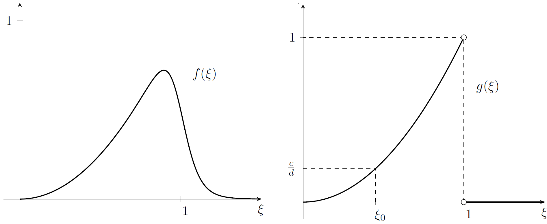
Figure 1: The shape of functions $f(\xi)=\frac{\xi^{k}}{1+\xi^{n}}$ (left) and $g(\xi)=\xi^{k}$ (right) satisfying conditions (F) and (G) respectively in case $k=2$.

The idea of this paper originates from [2] where $f(\xi)=\frac{\xi}{1+\xi^{n}}$ was the Mackey–Glass nonlinearity with $g(\xi)=\xi$ for $\xi\in[0,1)$, $g(\xi)=0$ for $\xi>1$. In [2] the linearity of $g$ in $[0,1)$ was essential to construct complicated looking periodic solutions of ($E_{g}$).

Here we extend [2] to all nonlinearities $f$ close to $g$ satisfying only condition (G). This includes not only the prototype nonlinearities (1.2) and (1.3) for large $n$, but also a large class of other unimodal nonlinearities. In addition, for the prototype nonlinearities (1.2) and (1.3), a threshold number can be explicitly constructed so that the results are valid if $n$ is larger than the threshold number.

Most of the periodic orbits obtained here do not seem to come from local or global Hopf bifurcations. Projecting the periodic solution $q$ into the plane by $t\mapsto(q(t),q(t-1))\in\mathbb{R}^{2}$ produce complicated looking figures for some periodic solutions $q$, although the corresponding periodic orbits are stable.

The region of attraction of the stable periodic orbit of ($E_{f}$) is estimated as well. Therefore we rigorously show bistability for the prototype nonlinearities if $k>1$. One stable attractor is the trivial equilibrium $0$, the other one is the obtained stable periodic orbit.

We expect that this paper with [2] opens up a new direction to study a wide class of delay differential equations with nonlinearities close to $g$. In particular, in forthcoming papers, motivated by the numerical results of [35], we consider the nonlinearity $f(\xi)=\frac{\xi^{2}}{1+\xi^{n}}$ modeling Allee effect, prove connections from equilibria to periodic orbits and between periodic orbits, moreover, we show the existence of homoclinic orbits. By the approach of the present paper and [2] we hope to prove rigorously complicated dynamics for the prototype nonlinearities for large values of $n$. Remark that the paper [15] constructed homoclinic orbits for certain unimodal nonlinearities, however not including (1.2), (1.3), and not having the spectral condition expected to be necessary for Shilnikov chaos.

Now we give the main results of the paper by using more technicalities. Let $g^{-1}$ denote the inverse of the restriction $g|_{[0,1)}$. The following property of Equation ($E_{g}$) plays an important role.

1. The parameters $d>c>0$ and the function $g$ are given such that (G) holds and Equation ($E_{g}$) has a periodic solution $p:\mathbb{R}\to(0,\infty)$ with minimal period $\omega_{p}>0$, and

   1. $p(0)=1$, $p(t)>1$ for all $t\in[-1,0)$;

   2. $(p(t),p(t-1))\neq\left(1,g^{-1}\left(\frac{c}{d}\right)\right)$ for all $t\in[0,\omega_{p}]$.

Set $\mathcal{O}_{p}=\{{p}_{t}:\,t\in[0,\omega_{p}]\}$, the orbit of $p$.

In order to define the closeness of $f$ to the discontinuous $g$, for a function $u:I\to\mathbb{R}$, given on an interval $I$, introduce

$$\|u\|_{I}=\sup_{\xi\in I}|u(\xi)|.$$

The main result can be formulated as follows.

Theorem 1.1.

Suppose that property (P) holds. Choose $\kappa_{1}>0$, $\kappa_{2}>0$ such that $p(\mathbb{R})\subset(\kappa_{1},\kappa_{2})$, and let $m=\left[\omega_{p}\right]$ be the integer part of $\omega_{p}$. There exists an $\varepsilon>0$ so that if $a,b,f$ are close to $c,d,g$, respectively, in the sense that

• $|a-c|<\varepsilon,\quad|b-d|<\varepsilon,$

• $\|f-g\|_{[\kappa_{1},1-\varepsilon]\cup[1+\varepsilon,\kappa_{2}]}<\varepsilon$,

• $\|f^{\prime}\|_{[1+\varepsilon,\kappa_{2}]}\left(\|f^{\prime}\|_{[\kappa_{1},\kappa_{2}]}\right)^{m}<\varepsilon$,

then equation ($E_{f}$) has a periodic solution $q:\mathbb{R}\to(\kappa_{1},\kappa_{2})$, with minimal period $\omega_{q}$ so that $|\omega_{p}-\omega_{q}|<\varepsilon$, and ${\mathcal{O}_{q}}=\{{q}_{t}:\,t\in[0,\omega_{q}]\}$ is hyperbolic, orbitally stable, exponentially attractive with asymptotic phase, and $\mathrm{dist}\,({\mathcal{O}_{p}},\mathcal{O}_{q})<\varepsilon.$ In addition, the set

$$\{\psi\in C^{+}:\quad\psi(s)\in[1+\varepsilon,\kappa_{2}]\text{ for all }s\in[-1,0]\}$$

belongs to the region of attraction of $\mathcal{O}_{q}$.

In Section 3, first a more technical version of Theorem 1.1 will be shown, see Theorem 3.1. The constants in Theorem 3.1 expressing the closeness of $a,b,f$ to $c,d,g$ are constructed explicitly in terms of the properties of the periodic solution $p$ given in (P), see Sections 2–3.

Condition (3) of Theorem 1.1 is satisfied if the derivative $f^{\prime}$ of $f$ is small on $[1+\varepsilon,\kappa_{2}]$ compared to $f^{\prime}$ on $[\kappa_{1},\kappa_{2}]$. This together with condition (2) requires that $f$ is close to $g$ in the $C^{1}$-norm on $[1+\varepsilon,\kappa_{2}]$. In particular, for $f_{n}(\xi)=\frac{\xi^{k}}{1+\xi^{n}}$ with a fixed $k>0$, $|f_{n}^{\prime}(\xi)|\leq K_{0}n$ on $[\kappa_{1},\kappa_{2}]$, and $|f_{n}^{\prime}(\xi)|\leq\frac{K_{0}n}{1+(1+\varepsilon)^{n}}$ on $[1+\varepsilon,\kappa_{2}]$, for some $K_{0}$, see Section 3.1. Therefore, condition (3) holds for large $n$. Our result does not work for the nonlinearity $f(\xi)=\xi e^{-\xi}$ because of the lack of condition (3).

Theorems 1.1 and 3.1 can guarantee the existence of a stable periodic orbit only if property (P) holds. In Section 4 an analytic proof shows that (P) is always satisfied if $d$ is sufficiently large compared to $c$, namely

$$d>\max\left\{\dfrac{e^{2c}-1}{I_{cg}},\dfrac{c}{g(e^{-c})}\right\}$$ (1.4)

where $I_{cg}=\int_{1}^{2}e^{cs}g(e^{-c(s-1)})\,ds$. By Lemma 4.2 the existence of a periodic solution with (P1) and $d>\frac{c}{g(e^{-c})}$ combined imply $p(t)\geq e^{-c}$ for all $t\in\mathbb{R}$. Hence

$$\xi\in[e^{-c},1) \ \text{ implies }\ -c+dg(\xi)\geq-c+dg(e^{-c})>0,$$

$$\xi>1 \ \text{ implies }\ -c+dg(\xi)=-c<0,$$

that is, a negative feedback condition holds with respect to $\xi=1$, see [8]. In this case property (P1) of $p$ and slow oscillation combined yield that three consecutive zeros of $p(t)-1$ determine $\omega_{p}$, and (P2) holds as well. Consequently, under condition (1.4), Theorems 1.1 and 3.1 give the existence of a stable slowly oscillating periodic solution $q$ of Equation ($E_{f}$), and the projected curves $t\mapsto(p(t),p(t-1))$ are relatively simple.

The rigorous, computer-assisted verification of property (P) in Section 5 is an essential part of this paper. Indeed, Section 5 developes a rigorous numerical technique to verify property (P) for some given $c,d,g$ in Equation ($E_{g}$). For several examples where (P) is satisfied, the obtained periodic solution $p$ can be complicated in the sense that the projected curves $t\mapsto(p(t),p(t-1))$ look complicated, similar to the numerically observed chaotic situations obtained in earlier papers. Notice that the complexity of $p$ implies that of $q$. We emphasize that the analogous computer-assisted proof in [2] was much simpler, since the fact $g(\xi)=\xi$, $\xi\in[0,1)$, allowed the search for periodic solutions, in local coordinates, in the class of functions $s\mapsto\sum_{j=0}^{N}a_{j}s^{j}e^{-cs}$. The particular form of $g$ makes it possible to verify property (P) for some parameters $d>c>0$. Property (P) is the same as hypothesis (H) in [2] for the case $g(\xi)=\xi$, $\xi\in[0,1)$, and $g(\xi)=0$ for $\xi>1$. It is nontrivial to extend the verification of (P) from the piece-wise linear $g$ of [2] to a general $g$ satisfying (G). The method of Section 5 achives this for a wide class of functions $g$, such that they can be represented on $(0,1)$ as a composition of simple functions such as arithmetic operators and well know functions, such as $\exp$, $\sin$, $\cos$, $\sqrt{\cdot}$, etc.

Property (P1) implies $p(t)=e^{-ct}$ for $t\in[0,1]$. The values of $p$ on $[0,1]$ determine uniquely $p$ on $[1,\infty)$. Therefore, $p$ is unique if it exists. From a solution $x:[0,\infty)\to\mathbb{R}$ of Equation ($E_{g}$) with $x(t)=e^{-ct}$ for $t\in[0,1]$ one easily finds a periodic $p$ with property (P1) if $x(t)>1$ for all $t\in[T,T+1]$ for some $T>1$, see Remark 1. The meaning of (P2) is that the orbit passes through the hyperplane $\{\phi\in C([-1,0],\mathbb{R}):\phi(0)=1\}$ transversally. Property (P2) guarantees that the measure of those times $t\in[0,\omega_{p}]$ is small, where $p(t)$ is close to the discontinuity point $\xi=1$ of $g$. This fact is crucial in the estimation of the difference between the periodic solution of Equation ($E_{g}$) and a solution of Equation ($E_{f}$), see Proposition 2.6. We remark that the idea of considering a simple nonlinear feedback function and nearby nonlinearities was applied in earlier works in the case when the nonlinearity $g$ was piece-wise constant, see e.g. [3], [12], [19], [20], [21], [36], [40], [45], [46], [47]. In the piece-wise constant situation the search for periodic solutions can be reduced to a finite dimensional problem. Our case is different since $g$ is not a step function on $[0,1)$, and the search for periodic solutions is still an infinite dimensional problem. Mackey et al. [32] applied a limiting technique, similar to the work and [2], for an equation including the Mackey–Glass nonlinearity $\frac{\xi}{1+\xi^{n}}$, and obtained simple looking stable periodic solutions.

2 Preliminary results

In this section we assume that $b>a>0$, $d>c>0$, and conditions (F) and (G) hold.

We use the notation $\mathbb{R}$ for the set of all real numbers, $\mathbb{N}$ for the set $\{1,2,\dots\}$, and let $\mathbb{N}_{0}=\{0\}\cup\mathbb{N}$.

Let $C$ denote the Banach space $C([-1,0],\mathbb{R})$ with the norm $\|\phi\|=\max_{s\in[-1,0]}|\phi(s)|$. For an interval $I$, $t-1,t\in I$ and a continuous function $u:I\to\mathbb{R}$, $u_{t}\in C$ is given by $u_{t}(s)=u(t+s)$, $-1\leq s\leq 0$. Introduce the subsets of $C$:

$$C^{+}=\{\psi\in C:\psi(s)\geq 0,\ s\in[-1,0]\},\quad C^{+}_{*}=\{\psi\in C^{+}:\psi^{-1}(c)\text{ is finite for }c\in(0,1]\}$$

where $\psi^{-1}(c)=\{s\in[-1,0]:\psi(s)=c\}$.

A solution of Equation ($E_{f}$) on $[-1,\infty)$ with initial function $\psi\in C^{+}$ is a continuous function $y=y^{\psi}:[-1,\infty)\to\mathbb{R}$ so that $y_{0}=\psi$, the restriction $y|_{(0,\infty)}$ is differentiable, and equation ($E_{f}$) holds for all $t>0$. The solutions are easily obtained from the variation-of-constants formula for ordinary differential equations on successive intervals of length one, that is

$$y(t)=e^{-a(t-j)}y(j)+b\int_{j}^{t}e^{-a(t-s)}f(y(s-1))\,ds,$$ (2.1)

where $j\in\mathbb{N}_{0}$, $j\leq t\leq j+1$. Each $\psi\in C^{+}$ as an initial function uniquely determines a solution $y=y^{\psi}:[-1,\infty)\to\mathbb{R}$ with $y_{0}^{\psi}=\psi$, and $y^{\psi}_{t}\in C^{+}$ for all $t\geq 0$. It is easy to see that $\psi\in C^{+}$, $\psi(0)>0$ imply $y^{\psi}(t)>0$ for all $t>0$. The solutions define the continuous semiflow

$$\Phi:[0,\infty)\times C^{+}\ni(t,\psi)\mapsto y_{t}^{\psi}\in C^{+}.$$

The discontinuity of $g$ requires a slightly different definition of a solution for ($E_{g}$). A solution of Equation ($E_{g}$) with an initial function $\phi\in C^{+}$ is a continuous function $x=x^{\phi}:[-1,t_{\phi})\to\mathbb{R}$ with some $0<t_{\phi}\leq\infty$ such that $x_{0}=\phi$, the map $[0,t_{\phi})\ni s\mapsto g(x(s-1))\in\mathbb{R}$ is locally integrable, and

$$x(t)=e^{-c(t-j)}x(j)+d\int_{j}^{t}e^{-c(t-s)}g(x(s-1))\,ds$$ (2.2)

holds for all $j\in\mathbb{N}_{0}$ and $t\in[0,t_{\phi})$ with $j\leq t\leq j+1$. It is not difficult to prove that, for any $\phi\in C^{+}$, there is a unique solution $x^{\phi}$ of Equation ($E_{g}$) on $[-1,\infty)$. For $u\in(-1,1)$ and for the inititial function $\phi(s)=1+u$, the solution $x^{u}$ of Equation ($E_{g}$) is

$$x^{u}(t)=e^{-ct}(1+u)+\dfrac{d}{c}g(1+u)[1-e^{-c}]\qquad(t\in[0,1],$$

see [2]. If continuity holds on initial functions in $C^{+}$, then

$$\lim_{u\to 0-}x^{u}(t)=x^{0}(t)=\lim_{u\to 0+}x^{u}(t)\qquad\text{for all }t\in[0,1].$$

This is impossible since, by (G), $\lim_{u\to 0-}g(1+u)>0$, $\lim_{u\to 0+}g(1+u)=0$. Consequently, in $C^{+}$ there is no continuous dependence on initial functions for Equation ($E_{g}$). This fact motivates the introduction of $C^{+}_{*}$ as a phase space for equation ($E_{g}$).

The proof of the following result requires only a straightforward modification of the proof of Proposition 2.2 in [2], therefore it is omitted here.

Proposition 2.1.

For all $\phi\in C^{+}_{*}$, Equation ($E_{g}$) has a unique solution $x^{\phi}$ on $[-1,\infty)$ with $x_{t}^{\phi}\in C^{+}_{*}$ for all $t\geq 0$. If $t>0$ and $x^{\phi}(t-1)\neq 1$, then $x^{\phi}$ is differentiable at $t$, and equation ($E_{g}$) holds at $t$. The map $\Gamma:[0,\infty)\times C^{+}_{*}\ni(t,\phi)\mapsto x_{t}^{\phi}\in C^{+}_{*}$ is a continuous semiflow.

We remark that, for $\psi\in C^{+}$ and $\phi\in C^{+}_{*}$, the unique solutions $y^{\psi}$ and $x^{\phi}$ of ($E_{f}$) and ($E_{g}$) satisfy the integral equations

$$y^{\psi}(t)=e^{-a(t-\tau)}y^{\psi}(\tau)+b\int_{\tau}^{t}e^{-a(t-s)}f(y^{\psi}(s-1))\,ds\qquad(0\leq\tau<t<\infty)$$ (2.3)

and

$$x^{\phi}(t)=e^{-c(t-\tau)}x^{\phi}(\tau)+d\int_{\tau}^{t}e^{-c(t-s)}g(x^{\phi}(s-1))\,ds\qquad(0\leq\tau<t<\infty),$$ (2.4)

respectively.

The following boundedness result is analogous to Proposition 2.3 in [2], and its proof is omitted:

Proposition 2.2.

Let $\phi\in C_{*}^{+}$, $\psi\in C^{+}$, and let $x=x^{\phi}$, $y=y^{\psi}$ be the solutions of Equations ($E_{g}$) and ($E_{f}$), respectively.

• There exists $t_{*}(\phi)\geq 0$ so that $x(t)<d/c$ for all $t>t_{*}(\phi)$. If $\phi(0)<d/c$ then $x(t)<d/c$ for all $t\geq 0$.

• There exists $t_{**}(\psi)\geq 0$ so that $y(t)<b/a$ for all $t>t_{**}(\psi)$. If $\psi(0)<b/a$ then $y(t)<b/a$ for all $t\geq 0$.

Let $g^{-1}$ denote the inverse of $g|_{[0,1)}$. By (G), $g^{-1}$ is strictly increasing, continuous, $g^{-1}(0)=0$. Define

$$\xi_{0}=g^{-1}\left(\frac{c}{d}\right)\in(0,1).$$

Proposition 2.3.

For each $\delta_{0}\in(0,\min\{\xi_{0},1-\xi_{0}\})$ there exist $\delta_{1}\in(0,\delta_{0})$ and $\mu>0$ such that

$$|-cu+dg(v)|\geq\mu\text{ for all }(u,v)\in\left[1-\delta_{1},1+\delta_{1}\right]\times\left(\left[0,\xi_{0}-\delta_{0}\right]\cup\left[\xi_{0}+\delta_{0},\infty\right)\right).$$

Proof.

From condition (G), $d>c>0$, and the choice of $\xi_{0}$, there exists a $\mu>0$ so that $|-c+dg(v)|\geq 2\mu$ for all $v\in\left[0,\xi_{0}-\delta_{0}\right]\cup\left[\xi_{0}+\delta_{0},\infty\right)$. By continuity, it is easy to see that the stated inequality holds if $\delta_{1}$ is sufficiently small. ∎

Proposition 2.4.

Let $\delta>0$, $\ell\in\mathbb{N}_{0}$, $0<\nu_{1}<1$, $1+\delta<\nu_{2}$, and $\psi,\chi\in C^{+}$ be given such that for the solutions $y=y^{\psi}$ and $z=z^{\chi}$ of ($E_{f}$) the relations

$$\psi(s)\in[1+\delta,\nu_{2}],\ \chi(s)\in[1+\delta,\nu_{2}]\text{ for all }s\in[-1,0],$$

$$y(t)\in[\nu_{1},\nu_{2}],\ z(t)\in[\nu_{1},\nu_{2}]\text{ for all }t\in[0,\ell]$$

hold. Then, for all $t\in[0,\ell+1]$,

$$|y(t)-z(t)|\leq\left(|\psi(0)-\chi(0)|+b\|f^{\prime}\|_{[1+\delta,\nu_{2}]}\|\psi-\chi\|\right)\left[1+b\|f^{\prime}\|_{[\nu_{1},\nu_{2}]}\right]^{\ell}.$$ (2.5)

Proof.

From the integral equation (2.3) for $y=y^{\psi}$ and $z=z^{\chi}$ with $\tau=0$ and $t\in[0,1]$ we have

$$\left|y(t)-z(t)\right| \leq e^{-at}|\psi(0)-\chi(0)|+b\sup_{1+\delta\leq\xi\leq\nu_{2}}|f^{\prime}(\xi)|\int_{0}^{t}e^{-a(t-s)}|y(s-1)-z(s-1)|\,ds$$

$$\leq|\psi(0)-\chi(0)|+b\|f^{\prime}\|_{[1+\delta,\nu_{2}]}\left\|\psi-\chi\right\|,$$

that is, (2.5) holds for $\ell=0$. Suppose that $k\in\mathbb{N}$ and for all $t\in[0,k]$ the inequality

$$|y(t)-z(t)|\leq\left(\left|\psi(0)-\chi(0)\right|+b\|f^{\prime}\|_{[1+\delta,\nu_{2}]}\left\|\psi-\chi\right\|\right)\left[1+b\|f^{\prime}\|_{[\nu_{1},\nu_{2}]}\right]^{k-1}$$

is valid. Then

$$\|y_{k}-z_{k}\|\leq\left(\left|\psi(0)-\chi(0)\right|+b\|f^{\prime}\|_{[1+\delta,\nu_{2}]}\left\|\psi-\chi\right\|\right)\left[1+b\|f^{\prime}\|_{[\nu_{1},\nu_{2}]}\right]^{k-1}$$ (2.6)

holds as well. By using (2.6), from the integral equation (2.3) for $y$ and $z$ with $\tau=k$ and $t\in[k,k+1]$, we obtain

$$|y(t)-z(t)|\leq e^{-a(t-k)}|y(k)-z(k)|+b\sup_{\xi\in[\nu_{1},\nu_{2}]}|f^{\prime}(\xi)|\int_{k}^{t}e^{-a(t-s)}|y(s-1)-z(s-1)|\,ds$$

$$\leq \left[1+b\|f^{\prime}\|_{[\nu_{1},\nu_{2}]}\right]\|y_{k}-z_{k}\|$$

$$\leq \left(\left|\psi(0)-\chi(0)\right|+b\|f^{\prime}\|_{[1+\delta,\nu_{2}]}\left\|\psi-\chi\right\|\right)\left[1+b\|f^{\prime}\|_{[\nu_{1},\nu_{2}]}\right]^{k}.$$

Thus, by the principle of induction, inequality (2.6) is satisfied for all $k\in\{1,\ldots,\ell+1\}$, and the proof is complete. ∎

Suppose that the following property holds for Equation ($E_{g}$):

1. The parameters $d>c>0$ and the function $g$, satisfying (G), are given such that Equation ($E_{g}$) has a periodic solution $p:\mathbb{R}\to(0,\infty)$ with minimal period $\omega_{p}>0$, and

   • $p(0)=1$, $p(t)>1$ for all $t\in[-1,0)$;

   • $(p(t),p(t-1))\neq(1,\xi_{0})$ for all $t\in[0,\omega_{p}]$.

Remark 1.

Assume that (P) is satisfied.

• By Equation ($E_{g}$), $p(t)=e^{-ct}$, $t\in[0,1]$. Clearly, $p_{1}\in C^{+}_{*}$, and then by Proposition 2.1 and periodicity, $p_{t}\in C^{+}_{*}$ for all $t\in\mathbb{R}$. In addition, $\omega_{p}>2$ and $p$ is unique.

• For given $d>c>0$ and $g$ satisfying (G), we can look for $p$ in the following way. Let $\phi(s)=e^{-c(1+s)}$, $s\in[-1,0]$, and define $x:[0,\infty)\to\mathbb{R}$ by $x(t)=\Gamma(t,\phi)(-1)$. That is, $x$ is a solution of ($E_{g}$) on $[0,\infty)$ with initial function $x(t)=e^{-ct}$, $t\in[0,1]$. If there exists an $\omega>1$ so that $x(\omega)=1$ and $x(\omega+s)>1$ for all $s\in[-1,0)$, then clearly $x(\omega+t)=e^{-ct}$ for all $t\in[0,1]$, i.e., $x_{\omega+1}=x_{1}$. If $\omega$ is minimal with the above property then $p$ is the $\omega$-periodic extension of $x|_{[0,\omega]}$, and $\omega_{p}=\omega$.

• By the above remark, there is no $\omega\in(0,\omega_{p})$ such that $p(\omega)=1$ and $p(\omega+s)>1$ for all $s\in[-1,0)$.

• Clearly, $p(t)\geq e^{-ct}$ for all $t\geq 0$, and, by Proposition 2.2, $p(t)<d/c$ for all $t\geq 0$. Therefore, $p(t)\in(e^{-c\omega_{p}},d/c)$ for all $t\in\mathbb{R}$.

Now we define several constants related to (P) and used in the sequel. Let

$$p_{m}=\min_{t\in\mathbb{R}}p(t),\quad p_{M}=\max_{t\in\mathbb{R}}p(t).$$

It is easy to see that $0<e^{-c\omega_{p}}<p_{m}<1<p_{M}<d/c$. Choose $\kappa_{1},\kappa_{2}$ so that

$$0<\kappa_{1}<p_{m}<p_{M}<\kappa_{2}.$$

Let

$$m=\left[\omega_{p}\right]$$

be the integer part of $\omega_{p}$. Then $m\leq\omega_{p}<m+1$.

Observe that $p_{0}\in C^{+}_{*}$, and then $p_{t}\in C_{*}^{+}$ for all $t\geq 0$ by Proposition 2.1. This fact allows to define $k_{0}\in\mathbb{N}$ as the number of points in the set

$$\{t\in(0,\omega_{p}]:\,p(t)=1\}.$$

By (P2) and continuity, a $\delta_{0}\in(0,\min\{\xi_{0},1-\xi_{0}\})$ can be fixed so that

$$(p(t),p(t-1))\notin\left[1-\delta_{0},1+\delta_{0}\right]\times\left[\xi_{0}-\delta_{0},\xi_{0}+\delta_{0}\right]$$

for all $t\in\mathbb{R}$. By Proposition 2.3 there exist $\delta_{1}\in(0,\delta_{0})$ and $\mu>0$ such that

$$|-cu+dg(v)|\geq\mu\text{ for all }(u,v)\in\left[1-\delta_{1},1+\delta_{1}\right]\times\left(\left[0,\xi_{0}-\delta_{0}\right]\cup\left[\xi_{0}+\delta_{0},\infty\right)\right).$$

Consequently, if $t\in\mathbb{R}$ and $p^{\prime}(t)$ exists, then

$$|p(t)-1|\leq\delta_{1}\text{ implies }|p^{\prime}(t)|\geq\mu.$$ (2.7)

Define the constants

$$k_{1}=\dfrac{2(3k_{0}+2)}{\mu},\quad k_{2}=2+\dfrac{d}{c}+\left(d+\delta_{1}\right)\left(2+2k_{1}+\|g^{\prime}\|_{[\kappa_{1},1)}\right).$$

Set

$$\delta_{2}=\frac{1}{k_{2}^{m}}\min\left\{\frac{\delta_{1}}{2},p_{m}-\kappa_{1},\kappa_{2}-p_{M}\right\}.$$

Property (P1) and continuity of $p$ imply the existence of a $\gamma\in(0,m+1-\omega_{p})$ so that

$$p(t)>1\text{ for all }t\in[-1-\gamma,0).$$

Choose the positive constants $\varepsilon_{0}$ and $\varepsilon_{1}$ so that

$$\varepsilon_{0}\leq\min\left\{k_{2}^{m}\delta_{2},\dfrac{c}{2},\frac{e^{c\gamma}-1}{2},\frac{1}{2}\left(\min_{t\in[-1-\gamma,-\gamma]}p(t)-1\right)\right\}\text{ and }\varepsilon_{1}=\frac{\varepsilon_{0}}{k_{2}^{m}}.$$

The constants

$$\sigma_{0}=\frac{1}{c}\log\frac{1+2\varepsilon_{0}}{1+\varepsilon_{0}},\quad\sigma_{1}=\frac{1}{c}\log(1+\varepsilon_{0})$$ (2.8)

satisfy $\sigma_{0}+\sigma_{1}=(1/c)\log(1+2\varepsilon_{0})\leq\gamma<m+1-\omega_{p}$ because of the choice of $\varepsilon_{0}$. Observe that $p(t)>1$, $t\in[-1-\gamma,0)$, $p(0)=1$ imply $p(t)=e^{-ct}$ for all $t\in[-\gamma,1]$. It follows that

$$p(-\sigma_{0}-\sigma_{1})=1+2\varepsilon_{0},\quad p(-\sigma_{1})=1+\varepsilon_{0}.$$

Let us define the shifted version of $p$ by

$$r:\mathbb{R}\ni t\mapsto p(t-\sigma_{1})\in\mathbb{R}.$$

Then $r$ is an $\omega_{p}$-periodic solution of ($E_{g}$) satisfying

$$\begin{split}r(t)&=(1+\varepsilon_{0})e^{-ct}\quad\text{ for all }t\in[-\sigma_{0},1+\sigma_{1}],\\ r(-\sigma_{0})&=1+2\varepsilon_{0},\quad r(0)=1+\varepsilon_{0},\quad r(\sigma_{1})=1,\\ r(t)&\geq 1+2\varepsilon_{0}\quad\text{ for all }t\in[-1-\sigma_{0},-\sigma_{0}].\end{split}$$ (2.9)

For $\delta\in(0,\delta_{1})$ let

$$\Delta(\delta)=\left\{t\in[0,m]:\,|r(t)-1|<\delta\right\}.$$

By the continuity of $r$, $\Delta(\delta)$ is an open set in $[0,m]$, and $\Delta(\delta)\cap(0,m)$ is the disjoint union of at most countable many open intervals. Let $|\Delta(\delta)|$ denote the sum of the lengths of these disjoint open intervals.

The next result shows that the measure of the set of those times $t$ for which $r(t)$ is close to the discontinuity $\xi=1$ of $g$ is small.

Proposition 2.5.

Suppose that (P) is satisfied. Then, for all $\delta\in(0,\delta_{1})$, the inequality

$$|\Delta(\delta)|\leq k_{1}\delta$$ (2.10)

holds.

Proof.

Let $\delta\in(0,\delta_{1})$ be given, and set $\Delta=\Delta(\delta)$.

By the definition of $k_{0}$, there are exactly $\ell_{0}\in\{1,\ldots,k_{0}\}$ points $t_{1},t_{2},\dots,t_{\ell_{0}}$ in $[0,m]$ such that $r(t_{j}-1)=1$, $j=1,2,\dots,\ell_{0}$. The set

$$(0,m)\cap\Delta\setminus\{t_{1},t_{2},\dots,t_{\ell_{0}}\}$$

is an open subset of $(0,m)$, and thus it is the disjoint union of at most countable many open intervals denoted by $\mathcal{I}$. Clearly, the sum of the lengths of the intervals in $\mathcal{I}$ is equal to $|\Delta|$.

Let $(\alpha,\beta)$ be an element of $\mathcal{I}$. By the choice of $\delta_{1}$ and by Propositions 2.1, 2.3 if $t\in(\alpha,\beta)$ then $r^{\prime}(t)$ exists, and by (2.7)

$$|r^{\prime}(t)|=|-cr(t)+dg(r(t-1))|\geq\mu.$$

Therefore, by continuity, either $r^{\prime}(t)\geq\mu$ for all $t\in(\alpha,\beta)$, or $r^{\prime}(t)\leq-\mu$ for all $t\in(\alpha,\beta)$. Then, for the length of the interval $(\alpha,\beta)$, one obtains

$$\beta-\alpha\leq\frac{1}{\mu}\left|\int_{\alpha}^{\beta}r^{\prime}(s)\,ds\right|=\frac{1}{\mu}\left|r(\beta)-r(\alpha)\right|\leq\frac{1}{\mu}|(1+\delta)-(1-\delta)|=\frac{2\delta}{\mu}.$$ (2.11)

For any $(\alpha,\beta)\in\mathcal{I}$ at least one of the five possibilities can occur:

• $\alpha=0$,

• $\beta=m$,

• $\alpha=t_{j}$ for some $j\in\{1,\ldots,\ell_{0}\}$,

• $\beta=t_{j}$ for some $j\in\{1,\ldots,\ell_{0}\}$,

• $[\alpha,\beta]\subset(0,m)$ and $[\alpha,\beta]\cap\{t_{1},t_{2},\dots,t_{\ell_{0}}\}=\emptyset$.

Case (i) (and similarly Case (ii)) can happen for at most one interval in $\mathcal{I}$. The number of intervals in $\mathcal{I}$, for which Case (iii) (and similarly Case (iv)) can hold, is at most $\ell_{0}\leq k_{0}$. For Case (v), from the fact that either $r^{\prime}(t)\geq\mu$ for all $t\in(\alpha,\beta)$, or $r^{\prime}(t)\leq-\mu$ for all $t\in(\alpha,\beta)$, it is easy to see that either $r(\alpha)=1-\delta$ and $r(\beta)=1+\delta$, or $r(\alpha)=1+\delta$ and $r(\beta)=1-\delta$. Thus, by continuity, there is a $t_{*}\in(\alpha,\beta)$ with $r(t_{*})=1$. By the definition of $k_{0}$, Case (v) may appear at most $k_{0}$ times.

Therefore, the set $(0,m)\cap\Delta\setminus\{t_{1},t_{2},\dots,t_{k_{0}}\}$ contains at most $2+2k_{0}+k_{0}=3k_{0}+2$ open intervals.

Finally, by applying (2.11), we conclude that

$$|\Delta|\leq(3k_{0}+2)\frac{2\delta}{\mu}=k_{1}\delta.$$

∎

The next result estimates the difference of the periodic solution $r$ of Equation ($E_{g}$) and a solution of Equation ($E_{f}$).

Proposition 2.6.

Suppose that property (P) holds, and for some $\delta\in(0,\delta_{2})$ the positive constants $a,b$, and the function $f$, in addition to (F), satisfy the conditions

• $|c-a|<\delta,\quad|d-b|<\delta$;

• $\|f-g\|_{[\kappa_{1},1-\delta]\cup[1+\delta,\kappa_{2}]}<\delta$.

Let $\psi\in C^{+}$ be given so that, for the solution $y=y^{\psi}$ of ($E_{f}$), the inequality

$$\|r_{1}-y_{1}\|<\delta$$

is valid. Then

$$\left|r(t)-y(t)\right|<\delta k_{2}^{m}\quad\text{ for all }t\in[0,m+1].$$

Proof.

It suffices to show that

$$\|r_{j}-y_{j}\|<\delta k_{2}^{j-1}$$ (2.12)

for all $j\in\{1,2,\dots,m+1\}$.

We prove by induction. According to the assumption $\|r_{1}-y_{1}\|<\delta$, statement (2.12) holds for $j=1$. Suppose that $j\in\{1,2,\ldots,m\}$, and (2.12) is satisfied. It remains to show that

$$\|r_{j+1}-y_{j+1}\|<\delta k_{2}^{j}.$$

By the choice of $\delta_{2}$,

$$\delta<\delta_{2}\leq\frac{1}{k_{2}^{m}}\min\{p_{m}-\kappa_{1},\kappa_{2}-p_{M}\}.$$

Hence, from the assumption $\|r_{j}-y_{j}\|<\delta k_{2}^{j-1}$, one finds $y(t)\in[\kappa_{1},\kappa_{2}]$ for all $t\in[j-1,j]$.

For $t\in[j,j+1]$ we have

$$r(t)=e^{-c(t-j)}r(j)+d\int_{j}^{t}e^{-c(t-s)}g(r(s-1))\,ds$$

and

$$y(t)=e^{-a(t-j)}y(j)+b\int_{j}^{t}e^{-a(t-s)}f(y(s-1))\,ds.$$

Using these integral equations, $g([0,\infty))\subset[0,1]$, the inequality $|e^{-cu}-e^{-au}|\leq|c-a|$ for $0\leq u\leq 1$, $p_{M}<d/c$, and assumption (i), we obtain, for $j\leq t\leq j+1$, that

$$\left|r(t)-y(t)\right| \leq\left|e^{-c(t-j)}-e^{-a(t-j)}\right|r(j)+e^{-a(t-j)}\left|r(j)-y(j)\right|$$

$$+|d-b|\int_{j}^{t}e^{-c(t-s)}g(r(s-1))\,ds+b\int_{j}^{t}\left|e^{-c(t-s)}-e^{-a(t-s)}\right|g(r(s-1))\,ds$$

$$+b\int_{j}^{t}e^{-a(t-s)}\left|g(r(s-1))-f(y(s-1))\right|\,ds$$

$$\leq|c-a|r(j)+\|r_{j}-y_{j}\|+|d-b|+(d+\delta)|c-a|$$

$$+(d+\delta)\int_{j}^{j+1}\left|g(r(s-1))-f(y(s-1))\right|\,ds$$

$$\leq\delta\left(\dfrac{d}{c}+1+k_{2}^{j-1}+(d+\delta)\right)+(d+\delta)\int_{j-1}^{j}\left|g(r(s))-f(y(s))\right|\,ds.$$

Let

$$\Delta_{j}(\delta)=\{t\in[j-1,j]:\quad|r(t)-1|<2\delta k_{2}^{j-1}\}.$$

Then, as $2\delta k_{2}^{j-1}<2\delta_{2}k_{2}^{m}\leq\delta_{1}$, by Proposition 2.5, we have $|\Delta_{j}(\delta)|\leq 2\delta k_{2}^{j-1}k_{1}$. Hence

$$\int_{\Delta_{j}(\delta)}\left|g(r(s))-f(y(s))\right|\,ds\leq|\Delta_{j}(\delta)|\leq 2k_{2}^{j-1}k_{1}\delta$$

since $|g(r(s))-f(y(s))|\leq 1$ for all $s\in[j-1,j]$. Let us define

$$S_{+}=\{t\in[j-1,j]:\quad r(t)\geq 1+2\delta k_{2}^{j-1}\},$$

$$S_{-}=\{t\in[j-1,j]:\quad r(t)\leq 1-2\delta k_{2}^{j-1}\}.$$

From the inductive hypothesis $\|r_{j}-y_{j}\|<\delta k_{2}^{j-1}$, it follows that

$$1+\delta k_{2}^{j-1}<y(s)\leq\kappa_{2}\quad\text{ for all }s\in S_{+},$$

and

$$\kappa_{1}\leq y(s)<1-\delta k_{2}^{j-1}\quad\text{ for all }s\in S_{-}.$$

For $s\in S_{+}$ we have

$$\left|g(r(s))-f(y(s))\right| =f(y(s))\leq\|f\|_{[1+\delta k_{2}^{j-1},\kappa_{2}]}\leq\|f\|_{[1+\delta,\kappa_{2}]}$$

$$=\|g-f\|_{[1+\delta,\kappa_{2}]}<\delta.$$

If $s\in S_{-}$ then

$$\left|g(r(s))-f(y(s))\right| \leq\left|g(r(s))-g(y(s))\right|+\left|g(y(s))-f(y(s))\right|$$

$$\leq\|g^{\prime}\|_{[\kappa_{1},1]}|r(s)-y(s)|+\|g-f\|_{[\kappa_{1},1-\delta k_{2}^{j-1}]}$$

$$\leq\|g^{\prime}\|_{[\kappa_{1},1)}\|r_{j}-y_{j}\|+\|g-f\|_{[\kappa_{1},1-\delta]}$$

$$\leq\left(\|g^{\prime}\|_{[\kappa_{1},1)}k_{2}^{j-1}+1\right)\delta.$$

Therefore

$$\int_{j}^{j+1}\left|g(r(s-1)-f(y(s-1)))\right|\,ds\leq\delta\left(2k_{2}^{j-1}k_{1}+\|g^{\prime}\|_{[\kappa_{1},1)}k_{2}^{j-1}+1\right).$$

It follows that

$$\|r_{j+1}-r_{j+1}\| =\delta\left(k_{2}^{j-1}\left[1+(d+\delta)(2k_{1}+\|g^{\prime}\|_{[\kappa_{1},1)})\right]+\frac{d}{c}+2(d+\delta)+1\right).$$

Clearly, $1\leq k_{2}^{j-1}$, and thus

$$\frac{d}{c}+2(d+\delta_{1})+1\leq k_{2}^{j-1}\left(\frac{d}{c}+2(d+\delta_{1})+1\right).$$

Consequently,

$$\|x_{j+1}-y_{j+1}\| \leq\delta k_{2}^{j-1}\left(2+(d+\delta_{1})\left(2+2k_{1}+\|g^{\prime}\|_{[\kappa_{1},1)})+\frac{d}{c}\right)\right)=\delta k_{2}^{j}.$$

This completes the proof.∎

3 Periodic orbits

In this section we prove that equation ($E_{f}$) has a stable periodic orbit provided property (P) holds for Equation ($E_{g}$) and $a,b,f$ are close to $c,d,g$ in the sense given below.

In Section 2, for $d>c>0$ and a periodic solution $p$ of Equation ($E_{g}$) satisfying (P1) and (P2), we constructed the constants $p_{m},p_{M},\kappa_{1},\kappa_{2},m,k_{0},\delta_{0},\delta_{1},\mu,k_{2},\delta_{2},\gamma,\varepsilon_{0},\varepsilon_{1},\sigma_{0},\sigma_{1}$.

The following result is a version of Theorem 1.1 by formulating the closeness of $a,b,f$ to $c,d,g$ with the explicitly given constants $\varepsilon_{0},\varepsilon_{1},m$. First we prove Theorem 3.1, and then show that Theorem 1.1 is a consequence.

Theorem 3.1.

Let property (P) hold for Equation ($E_{g}$), and suppose that the positive constants $a,b$ and the function $f$ satisfy the conditions

• $|c-a|(1+\varepsilon_{0})<\frac{\varepsilon_{1}}{2},$

• $|d-b|<\varepsilon_{1},$

• $\|f-g\|_{[\kappa_{1},1-\varepsilon_{1}]\cup[1+\varepsilon_{1},\kappa_{2}]}<\varepsilon_{1},$

• $b\|f\|_{[1+\varepsilon_{0},\kappa_{2}]}<\frac{\varepsilon_{1}}{2},$

• $b\left(1+\frac{4b}{a}\right)\|f^{\prime}\|_{[1+\varepsilon_{0},\kappa_{2}]}\left(1+b\|f^{\prime}\|_{[\kappa_{1},\kappa_{2}]}\right)^{m}<1$.

Then equation ($E_{f}$) has a periodic solution $q:\mathbb{R}\to\mathbb{R}$, with minimal period $\omega_{q}>0$ satisfying $|\omega_{q}-\omega_{p}|<\frac{\varepsilon_{0}}{c}$, such that the periodic orbit $\mathcal{O}_{q}=\{q_{t}:\,t\in[0,\omega_{q}]\}$ is hyperbolic, orbitally stable, exponentially attractive with asymptotic phase, and $\mathrm{dist}\,(\mathcal{O}_{q},\mathcal{O}_{p})<\varepsilon_{0}.$ The set

$$U_{\varepsilon_{0},\kappa_{2}}=\{\psi\in C^{+}:\,\psi(s)\in[1+\varepsilon_{0},\kappa_{2}]\text{ for all }s\in[-1,0]\}$$

belongs to the region of attraction of $\mathcal{O}_{q}$. Moreover, if the stronger condition $b\|f\|_{[1+\varepsilon_{0},\infty)}<\frac{\varepsilon_{1}}{2}$ is satisfied instead of (iv), then the region of attraction of $\mathcal{O}_{q}$ contains

$$U_{\varepsilon_{0},\infty}=\{\psi\in C^{+}:\,\psi(s)\geq 1+\varepsilon_{0}\text{ for all }s\in[-1,0]\}.$$

Proof.

Define

$$S_{\varepsilon_{0},\kappa_{2}}=\{\psi\in C:\,\psi(0)=1+\varepsilon_{0},\psi(s)\in[1+\varepsilon_{0},\kappa_{2}]\text{ for all }s\in[-1,0]\}.$$

Let $b>a>0$ and $f$ be given such that conditions (i)-(v) are satisfied. Let $\psi\in S_{\varepsilon_{0},\kappa_{2}}$, and let $y=y^{\psi}$ be the solution of ($E_{f}$).

Step 1: Proof of

$$|r(t)-y(t)|<\varepsilon_{1}k_{2}^{m}=\varepsilon_{0}\quad\text{ for all }t\in[0,m+1].$$ (3.1)

For $t\in[0,1]$ we have

$$r(t)=e^{-ct}r(0)=e^{-ct}(1+\varepsilon_{0}),$$

$$y(t)=e^{-at}(1+\varepsilon_{0})+b\int_{0}^{t}e^{-a(t-s)}f(y(s-1))\,ds.$$

Hence, by conditions (i) and (iv), for all $t\in[0,1]$,

$$|r(t)-y(t)| \leq|e^{-ct}-e^{-at}|(1+\varepsilon_{0})+b\int_{0}^{1}f\left(\psi(s-1)\right)\,ds$$

$$\leq|c-a|(1+\varepsilon_{0})+b\|f\|_{[1+\varepsilon_{0},\kappa_{2}]}<\varepsilon_{1},$$

that is $\|r_{1}-y_{1}\|<\varepsilon_{1}$.

Observe that $\varepsilon_{1}=\varepsilon_{0}/k_{2}^{m}\leq\delta_{2}$. Conditions (i)–(iii) of the theorem imply (i) and (ii) of Proposition 2.6 with $\delta=\varepsilon_{1}$. The assumption $\|r_{1}-y_{1}\|<\delta$ of Proposition 2.6 holds as well. Consequently (3.1) is satisfied.

Step 2: Properties of $y$.

Combining properties (2.9) of $r$, inequality (3.1), the choice of $\varepsilon_{0}$, $r(\mathbb{R})=[p_{m},p_{M}]$, $\omega_{p}<m+1$, it follows that

$$\begin{split}&y(t)\in(r(t)-\varepsilon_{0},r(t)+\varepsilon_{0})\subset[p_{m}-\varepsilon_{0},p_{M}+\varepsilon_{0}]\subset(\kappa_{1},\kappa_{2})\quad(0\leq t\leq m+1),\\ &y(\omega_{p}-\sigma_{0})>r(\omega_{p}-\sigma_{0})-\varepsilon_{0}=r(-\sigma_{0})-\varepsilon_{0}=1+\varepsilon_{0},\\ &y(\omega_{p}+\sigma_{1})<r(\omega_{p}+\sigma_{1})+\varepsilon_{0}=r(\sigma_{1})+\varepsilon_{0}=1+\varepsilon_{0},\\ &y(t)>r(t)-\varepsilon_{0}\geq 1+2\varepsilon_{0}-\varepsilon_{0}=1+\varepsilon_{0}\quad(t\in[\omega_{p}-1-\sigma_{0},\omega_{p}-\sigma_{0}]),\\ &y(t)>r(t)-\varepsilon_{0}\geq 1-\varepsilon_{0}\quad(t\in[\omega_{p}-\sigma_{0},\omega_{p}+\sigma_{1}]).\end{split}$$ (3.2)

Step 3: A return map.

By using the first and the last inequality in (LABEL:y-properties) and condition (iv), we have

$$y^{\prime}(t)=-ay(t)+bf(y(t-1))<-a(1-\varepsilon_{0})+\frac{\varepsilon_{1}}{2}\ \text{ for all }t\in[\omega_{p}-\sigma_{0},\omega_{p}+\sigma_{1}].$$ (3.3)

From $\delta_{1}<\delta_{0}<1/2$ and $\varepsilon_{0}\leq k_{2}^{m}\delta_{2}\leq\delta_{1}/2$ one gets $\varepsilon_{0}<1/4$. From $\varepsilon_{0}\leq c/2$, $m\geq 1$, $k_{2}\geq 3$, it follows that $\varepsilon_{1}=\varepsilon_{0}/k_{2}^{m}<c/6$. From condition (i), clearly $|c-a|<\varepsilon_{1}/2$. Therefore

$$a>c-\frac{\varepsilon_{1}}{2}>c-\frac{c}{12}=\frac{11c}{12}>\frac{11}{2}\varepsilon_{1}.$$ (3.4)

From (3.3) with $\varepsilon_{0}<1/4$ and $\varepsilon_{1}<2a/11$, which comes from (3.4), we conclude

$$y^{\prime}(t)<-\frac{3}{4}a+\frac{a}{11}<-\frac{a}{2}\text{ for all }t\in[\omega_{p}-\sigma_{0},\omega_{p}+\sigma_{1}].$$ (3.5)

Consequently, $y$ strictly decreases on $[\omega_{p}-\sigma_{0},\omega_{p}+\sigma_{1}].$ From (LABEL:y-properties) one gets $y(\omega_{p}-\sigma_{0})>1+\varepsilon_{0}$ and $y(\omega_{p}+\sigma_{1})<1+\varepsilon_{0}$. Thus, by the strict monotonicity property of $y$ on $[\omega_{p}-\sigma_{0},\omega_{p}+\sigma_{1}]$, there is a unique $\tau=\tau(\psi)\in(\omega_{p}-\sigma_{0},\omega_{p}+\sigma_{1})$ so that $y(\tau)=1+\varepsilon_{0}$. By (LABEL:y-properties) it follows that $y_{\tau}\in S_{\varepsilon_{0},\kappa_{2}}.$

Now we can define a return map $R$ by

$$R:S_{\varepsilon_{0},\kappa_{2}}\ni\psi\mapsto y_{\tau}^{\psi}=\Phi(\tau(\psi),\psi)\in S_{\varepsilon_{0},\kappa_{2}}.$$

Step 4: The return map $R$ is a contraction.

Let $\psi,\chi\in S_{\varepsilon_{0},\kappa_{2}}$ and let $y=y^{\psi}$, $z=z^{\chi}$. We want to estimate $\|R(\psi)-R(\chi)\|$.

As $\psi\in S_{\varepsilon_{0},\kappa_{2}}$ was arbitrary in Steps 1–3, the results obtained in Steps 1–3 are valid for any element of $S_{\varepsilon_{0},\kappa_{2}}$. Then, by (LABEL:y-properties), $y(t),z(t)\in[\kappa_{1},\kappa_{2}]$, $t\in[-1,m+1]$. Applying Proposition 2.4 with $\delta=\varepsilon_{0}$, $\ell=m$, $\psi,\chi\in S_{\varepsilon_{0},\kappa_{2}}$ and $\psi(0)=\chi(0)=1+\varepsilon$, we obtain

$$|y(t)-z(t)|\leq b\|f^{\prime}\|_{[1+\varepsilon_{0},\kappa_{2}]}\left(1+b\|f^{\prime}\|_{[\kappa_{1},\kappa_{2}]}\right)^{m}\|\psi-\chi\|\quad\text{ for all }t\in[0,m+1].$$ (3.6)

In order to estimate $\tau(\psi)-\tau(\chi)$, observe that $y(\tau(\psi))=1+\varepsilon_{0}=z(\tau(\chi))$, and $\tau(\psi),\tau(\chi)\in(\omega_{p}-\sigma_{0},\omega_{p}+\sigma_{1})$. Hence and from (3.5) and (3.6) it follows that

$$\begin{split}|\tau(\psi)-\tau(\chi)|&=\left|\int_{\tau(\chi)}^{\tau(\psi)}1\,dt\right|<\frac{2}{a}\left|\int_{\tau(\chi)}^{\tau(\psi)}y^{\prime}(t)\,dt\right|=\frac{2}{a}|y(\tau(\psi))-y(\tau(\chi))|\\ &=\frac{2}{a}|z(\tau(\chi))-y(\tau(\chi))|\leq\frac{2b}{a}\|f^{\prime}\|_{[1+\varepsilon_{0},\kappa_{2}]}\left(1+b\|f^{\prime}\|_{[\kappa_{1},\kappa_{2}]}\right)^{m}\|\psi-\chi\|.\end{split}$$ (3.7)

By Proposition 2.2, $y(t)<b/a$ for all $t\geq 0$, and then $|y^{\prime}(t)|=|-ay(t)+bf(y(t-1))|<2b$ for all $t>0$. Thus $\|y_{\tau_{y}}-y_{\tau_{z}}\|\leq 2b|\tau_{y}-\tau_{z}|.$ Hence

$$\|\Phi(\tau(\psi),\psi)-\Phi(\tau(\chi),\psi)\|\leq 2b|\tau(\psi)-\tau(\chi)|.$$ (3.8)

Combining (3.8), (3.7) and (3.6) it follows that

$$\|R(\psi)-R(\chi)\| =\|\Phi(\tau(\psi),\psi)-\Phi(\tau(\chi),\chi)\|$$

$$\leq\|\Phi(\tau(\psi),\psi)-\Phi(\tau(\chi),\psi)\|+\|\Phi(\tau(\chi),\psi)-\Phi(\tau(\chi),\chi)\|$$

$$\leq 2b|\tau(\psi)-\tau(\chi)|+b\|f^{\prime}\|_{[1+\varepsilon_{0},\kappa_{2}]}\left(1+b\|f^{\prime}\|_{[\kappa_{1},\kappa_{2}]}\right)^{m}\|\psi-\chi\|$$

$$\leq b\left(1+\frac{4b}{a}\right)\|f^{\prime}\|_{[1+\varepsilon_{0},\kappa_{2}]}\left(1+b\|f^{\prime}\|_{[\kappa_{1},\kappa_{2}]}\right)^{m}\|\psi-\chi\|=\kappa\|\psi-\chi\|,$$

where

$$\kappa=b\left(1+\frac{4b}{a}\right)\|f^{\prime}\|_{[1+\varepsilon_{1},\kappa_{2}]}\left(1+b\|f^{\prime}\|_{[\varepsilon_{1},\kappa_{2}]}\right)^{m}<1$$

by condition (v). Therefore, $R:S_{\varepsilon_{0},\kappa_{2}}\to S_{\varepsilon_{0},\kappa_{2}}$ is a contraction.

Step 5: The periodic orbit.

The closed subset $S_{\varepsilon_{0},\kappa_{2}}$ of $C$ is a complete metric space with the metric induced by the norm of $C$. By Step 4, $R:S_{\varepsilon_{0},\kappa_{2}}\to S_{\varepsilon_{0},\kappa_{2}}$ is a contraction, and has a unique fixed point $\phi^{*}$ in $S_{\varepsilon_{0},\kappa_{2}}$ satisfying

$$\phi^{*}=\Phi(\tau(\phi^{*}),\phi^{*})$$

with $\tau(\phi^{*})\in[\omega_{p}-\sigma_{0},\omega_{p}+\sigma_{1}]$. Then, for the solution $y^{*}=y^{\phi^{*}}:[-1,\infty)\to\mathbb{R}$ of Equation ($E_{f}$), $y^{*}(t)=y^{*}(t+\tau(\phi^{*}))$ for all $t\geq-1$. Let $\omega_{q}=\tau(\phi^{*})$, and let $q:\mathbb{R}\to\mathbb{R}$ be the $\omega_{q}$-periodic extension of $y^{*}$. Clearly, $q$ is an $\omega_{q}$-periodic solution of Equation ($E_{f}$).

As $\phi^{*}\in S_{\varepsilon_{0},\kappa_{2}}$, the estimations obtained for $y=y^{\psi}$ in Steps 1–3 are valid for $y^{*}$. Therefore,

$$\begin{split}&|q(t)-r(t)|<\varepsilon_{0}\quad(t\in[0,m+1]),\\ &q(t)>1+\varepsilon_{0}\quad(t\in[\omega_{p}-1-\sigma_{0},\omega_{p}-\sigma_{0}),\\ &q\text{ strictly decreases on }[\omega_{p}-\sigma_{0},\omega_{p}+\sigma_{1}].\end{split}$$ (3.9)

It easily follows that $\mathrm{dist}\,(\mathcal{O}_{q},\mathcal{O}_{p})<\varepsilon_{0}$, and

$$|\omega_{q}-\omega_{p}|<\max\{\sigma_{0},\sigma_{1}\}\leq\frac{\varepsilon_{0}}{c}.$$

The exponential attractivity and asymptotic phase properties of the solution $q$ are consequences of the contractivity of $R$ in the same way as in Chapter XIV of [8], and [2].

Step 6: Region of attraction.

As $R$ is a contraction on the complete metric space $S_{\varepsilon_{0},\kappa_{2}}$, the set $S_{\varepsilon_{0},\kappa_{2}}$ belongs to the region of attraction of $\mathcal{O}_{q}$.

For $\psi\in U_{\varepsilon_{0},\kappa_{2}}$, we claim that there is a $t_{*}\geq 0$ such that $y_{t_{*}}^{\psi}\in S_{\varepsilon_{0},\kappa_{2}}$.

If $\psi(0)=1+\varepsilon_{0}$, then the claim holds with $t_{*}=0$. Suppose $\psi(0)>1+\varepsilon_{0}$, and let $y=y^{\psi}$. Choose a maximal $T\in(0,\infty)\cup\{\infty\}$ so that $y(t)>1+\varepsilon_{0}$ for all $t\in(0,T)$.

Define the sequence $(t_{k})$ by $t_{0}=0$, $t_{k}=\min\{t_{k-1}+1,T\}$, $k\in\mathbb{N}$. By using $y_{0}=\psi\in U_{\varepsilon_{0},\kappa_{2}}$, condition (iv), and (3.4), we obtain that

$$y^{\prime}(t)=-ay(t)+bf(\psi(t-1))<-a(1+\varepsilon_{0})+\frac{\varepsilon_{1}}{2}<-\frac{11}{2}\varepsilon_{1}+\frac{\varepsilon_{1}}{2}=-5\varepsilon_{1}$$

for all $t\in(0,t_{1}]$. Hence, $y$ strictly decreases on $[t_{0},t_{1}]$, and either $y_{t_{1}}\in S_{\varepsilon_{0},\kappa_{2}}$, or $y(t_{1})>1+\varepsilon_{0}$ and $y_{t_{1}}\in U_{\varepsilon_{0},\kappa_{2}}$. If $k\in\mathbb{N}$ and $y(t_{k})>1+\varepsilon_{0}$ and $y_{t_{k}}\in U_{\varepsilon_{0},\kappa_{2}}$, then in the same way as above, $y^{\prime}(t)<-5\varepsilon_{1}$ follows for all $t\in(t_{k},t_{k+1}]$. Repeating this process, we either find a $k\in\mathbb{N}$ so that the claim holds with $t_{*}=t_{k}$, or

$$y(t)>1+\varepsilon_{0},\quad y^{\prime}(t)<-5\varepsilon_{1}\text{ for all }t>0,$$

which is a contradiction.

Therefore, the claim holds, and consequently $U_{\varepsilon_{0},\kappa_{2}}$ is also in the region of attraction of $\mathcal{O}_{q}$.

If $\chi\in U_{\varepsilon_{0},\infty}$ and $b\|f\|_{1+\varepsilon_{0},\infty)}<\varepsilon_{1}/2$ holds, then following the proof of the above claim, a $t_{*}\geq 0$ can be obtained so that $y^{\chi}(t_{*})=1+\varepsilon_{0}$ and $y^{\chi}(t_{*}+s)\geq 1+\varepsilon_{0}$, $-1\leq s\leq 0$. Choose $\psi=y_{t_{*}}^{\chi}$ as an initial function of the solution $y=y^{\psi}$ of Equation ($E_{f}$). Then, although $\psi$ may not be in $S_{\varepsilon_{0},\kappa_{2}}$, the stronger condition $b\|f\|_{1+\varepsilon_{0},\infty)}<\varepsilon_{1}/2$ instead of (iv) allows to apply the above Steps 1–3 to find a $\tau>0$ with $y_{\tau}^{\psi}\in S_{\varepsilon_{0},\kappa_{2}}$. Therefore, $U_{\varepsilon_{0},\infty}$ belongs to the region of attraction of $\mathcal{O}_{q}$.

Step 7: $\omega_{q}$ is the minimal period of $q$.

Assume that $\overline{\omega_{q}}\in(0,\omega_{q})$ is also a period of $q$, that is $q_{0}=q_{\overline{\omega_{q}}}$.

If $\overline{\omega_{q}}\in(0,1]$ then $q(t)\geq 1+\varepsilon_{0}$ follows for all $t\in\mathbb{R}$. This is impossible by (LABEL:q-properties) since $r(t)<1$ for $t\in(\sigma_{1},1+\sigma_{1}]$. The properties (LABEL:q-properties) of $q$ and $\omega_{q}\in[\omega_{p}-\sigma_{0},\omega_{p}+\sigma_{1}]$ imply that $\overline{\omega_{q}}<\omega_{p}-1-\sigma_{0}$. Therefore,

$$1<\overline{\omega_{q}}<\omega_{p}-1-\sigma_{0},$$

and $q(\overline{\omega_{q}})=1+\varepsilon_{0}$, $q(\overline{\omega_{q}}+s)\geq 1+\varepsilon_{0}$, $-1\leq s\leq 0$.

Applying (LABEL:q-properties), it follows that $r(t)>1$ for all $t\in[\overline{\omega_{q}}-1,\overline{\omega_{q}}]$, and $r(\overline{\omega_{q}})\in(1,1+2\varepsilon_{0})$. Then, from Equation ($E_{g}$), $r(t)=r(\overline{\omega_{q}})e^{-c(t-\overline{\omega_{q}})}$, $t\in[\overline{\omega_{q}},\overline{\omega_{q}}+1]$. Hence, by the choice of $\varepsilon_{0}$ and $\gamma\in(0,1)$, we get $r(\overline{\omega_{q}}+1)<(1+2\varepsilon_{0})e^{-c}<1$. Then there is a $\nu\in(\overline{\omega_{q}},\overline{\omega_{q}}+1)$ such that

$$r(\nu)=1,\quad r(\nu+s)>1\text{ for all }s\in[-1,0).$$

By Remark 1 and the definition of $r$, $\nu-\sigma_{1}$ is a period of $p$ . Clearly,

$$\nu-\sigma_{1}\in(1-\sigma_{1},\omega_{p}-\sigma_{0}-\sigma_{1})\subset(0,\omega_{p}),$$

a contradiction to the minimality of $\omega_{p}$. Consequently, $\omega_{q}$ is the minimal period of $q$. ∎

In the Introduction we formalized Theorem 1.1 in order to state the main result in a not too technical way. Now we show how to obtain Theorem 3.1 from Theorem 1.1.

Proof of Theorem 1.1.

Assume property (P), and choose $\kappa_{1},\kappa_{2},m,\delta_{0},\delta_{1},\mu,k_{0},k_{1},k_{2},\gamma,\varepsilon_{,}\varepsilon_{1}$ as in Section 2.

Let $\varepsilon\in(0,1)$ be so small that

$$g(1-\varepsilon)>4\varepsilon,$$

$$\varepsilon<\min\left\{\frac{\varepsilon_{1}}{2(1+\varepsilon_{0})},\frac{\varepsilon_{1}}{2(d+\varepsilon_{1})}\right\}$$

and

$$\varepsilon<\frac{1}{(d+\varepsilon_{1})\left(1+4\frac{d+\varepsilon_{1}}{c-\varepsilon_{1}}\right)(1+d+\varepsilon_{1})^{m}}.$$ (3.10)

Suppose that $a,b,f$ are given so that conditions (1),(2),(3) of Theorem 1.1 are satisfied. Then conditions (i),(ii) and (iii) of Theorem 3.1 hold since $\varepsilon<\frac{\varepsilon_{1}}{2(1+\varepsilon 0)}<\varepsilon_{1}$.

Combining the fact $g(\xi)=0$ for $\xi>1$, condition (2) of Theorem 1.1, $\varepsilon_{1}<\varepsilon_{0}$, the choice of $\varepsilon$, we obtain

$$b\|f\|_{[1+\varepsilon_{0},\kappa_{2}]}\leq b\|f\|_{[1+\varepsilon,\kappa_{2}]}<b\varepsilon<b\frac{\varepsilon_{1}}{2(d+\varepsilon_{1})}<\frac{\varepsilon_{1}}{2},$$

that is, condition (iv) in Theorem 3.1 is valid.

In order to show (v) of Theorem 3.1, from $\varepsilon<\varepsilon_{1}<\varepsilon_{0}$ obviously $\|f^{\prime}\|_{[1+\varepsilon_{0},\kappa_{2}]}\leq\|f^{\prime}\|_{[1+\varepsilon,\kappa_{2}]}$.

Observe that $\|f-g\|_{[\kappa_{1},1-\varepsilon]}<\varepsilon$ and $g(1-\varepsilon)>4\varepsilon$ imply $f(1-\varepsilon)>3\varepsilon$. From $\|f\|_{[1+\varepsilon,\kappa_{2}]}=\|f-g\|_{[1+\varepsilon,\kappa_{2}]}<\varepsilon$ one gets $f(1+\varepsilon)<\varepsilon$. Consequently, there is a $\xi\in(1-\varepsilon,1+\varepsilon)$ such that $f^{\prime}(\xi)<-2$, and thus $\|f^{\prime}\|_{[\kappa_{1},\kappa_{2}]}>1$.

From properties (i), (ii) of Theorem 3.1, and from (3.10) one has

$$b\left(1+\frac{4b}{a}\right)(1+b)^{m}\varepsilon<(d+\varepsilon_{1})\left(1+4\frac{d+\varepsilon_{1}}{c-\varepsilon_{1}}\right)(1+d+\varepsilon_{1})^{m}\varepsilon<1.$$ (3.11)

Assuming (3) of Theorem 1.1, using the above results and (3.11), it follows that

$$b\left(1+\frac{4b}{a}\right)\|f^{\prime}\|_{[1+\varepsilon_{0},\kappa_{2}]}\left(1+b\|f^{\prime}\|_{[\kappa_{1},\kappa_{2}]}\right)^{m}\leq b\left(1+\frac{4b}{a}\right)\|f^{\prime}\|_{[1+\varepsilon,\kappa_{2}]}\left(1+b\|f^{\prime}\|_{[\kappa_{1},\kappa_{2}]}\right)^{m}$$

$$=b\left(1+\frac{4b}{a}\right)\frac{\left(1+b\|f^{\prime}\|_{[\kappa_{1},\kappa_{2}]}\right)^{m}}{\left(\|f^{\prime}\|_{[\kappa_{1},\kappa_{2}]}\right)^{m}}\|f^{\prime}\|_{[1+\varepsilon,\kappa_{2}]}\left(\|f^{\prime}\|_{[\kappa_{1},\kappa_{2}]}\right)^{m}$$

$$<b\left(1+\frac{4b}{a}\right)\left(\frac{1}{\|f^{\prime}\|_{[\kappa_{1},\kappa_{2}]}}+b\right)^{m}\varepsilon<b\left(1+\frac{4b}{a}\right)(1+b)^{m}\varepsilon<1,$$

that is (v) of Theorem 3.1 holds. This completes the proof. ∎

3.1 Examples

We show that if $f$ is the nonlinearity given in (1.2), and $g(\xi)=\xi^{k}$, $0\leq\xi\leq 1$, $g(\xi)=0$, $\xi>1$, then, for any given $m\in\mathbb{N}$ and $\varepsilon,\kappa_{1},\kappa_{2}$ with $0<\kappa_{1}<1-\varepsilon<1+\varepsilon<\kappa_{2}$, conditions (2) and (3) of Theorem 1.1 hold provided $n$ is sufficiently large. Consequently, by the proof of Theorem 1.1, if (P) holds and $a,b$ are sufficiently close to $c,d$ then the conditions of Theorems 1.1 and 3.1 are satisfied for the prototype nonlinearity (1.2) provided $n$ is large enough.

Let $k>0$ be fixed, and for the parameter $n\geq k$ consider

$$f_{n}(\xi)=\frac{\xi^{k}}{1+\xi^{n}}\quad(\xi\geq 0),$$

and

$$g(\xi)=\begin{cases}\xi^{k}&\text{ if }\xi\in[0,1],\\ 0&\text{ if }\xi>1.\end{cases}$$

Function $g$ satisfies condition (G), and

$$\lim_{n\to\infty}f_{n}(\xi)=g(\xi)$$

for all $\xi\in[0,\infty)\setminus\{1\}$.

Claim.

Let $m\in\mathbb{N}$ and $\varepsilon,\kappa_{1},\kappa_{2}$ be given constants such that

$$0<\kappa_{1}<1-\varepsilon<1+\varepsilon<\kappa_{2}.$$

There exists an $N>0$ so that for the function $f=f_{n}$ assumption (F) and conditions (2),(3) of Theorem 1.1 are satisfied provided $n\geq N$.

Proof.

It is clear that $f_{n}(\xi)\leq 1$ for all $\xi\geq 0$, and $f_{n}(\xi)<1$ for $\xi>1$ since $n\geq k$.

For condition (2) of Theorem 1.1 we have to estimate $|g(\xi)-f_{n}(\xi)|$. If $\xi\leq 1-\varepsilon$, then

$$|g(\xi)-f_{n}(\xi)|=\left|\xi^{k}\frac{\xi^{n}}{1+\xi^{n}}\right|\leq\xi^{n}\leq(1-\varepsilon)^{n}<\varepsilon,\quad n>n_{1}(\varepsilon).$$

provided $n\geq N_{1}$ for some $N_{1}>0$.

If $\xi\geq 1+\varepsilon$ then

$$|g(\xi)-f_{n}(\xi)|=f_{n}(\xi)\leq\frac{\xi^{k}}{1+\xi^{k}\xi^{n-k}}=\frac{1}{\frac{1}{\xi^{k}}+\xi^{n-k}}<\frac{1}{\xi^{n-k}}<\frac{1}{(1+\varepsilon)^{n-k}}<\varepsilon$$

whenever $n\geq N_{2}$ for some $N_{2}\geq k$.

As $f_{n}^{\prime}(\xi)=\frac{k\xi^{k-1}}{1+\xi^{n}}-\frac{n\xi^{k}\xi^{n-1}}{(1+\xi^{n})^{2}}$, for $\xi>0$, by $n\geq k$ we have

$$|f^{\prime}_{n}(\xi)|\leq\xi^{k-1}(k+n)\leq 2n\max\{\kappa_{1}^{k-1},\kappa_{2}^{k-1}\}=K_{0}n\quad(\xi\in[\kappa_{1},\kappa_{2}]),$$

where $K_{0}=2\max\{\kappa_{1}^{k-1},\kappa_{2}^{k-1}\}$. For $\xi\in[1+\varepsilon,\kappa_{2}]$

$$|f_{n}^{\prime}(\xi)| \leq\frac{1}{1+\xi^{n}}\left|k\xi^{k-1}-n\xi^{k-1}\frac{\xi^{n}}{1+\xi^{n}}\right|$$

$$\leq\frac{1}{1+\xi^{n}}(n+k)\xi^{k-1}\leq(n+k)\max\{1,\kappa_{2}^{k-1}\}\frac{1}{1+(1+\varepsilon)^{n}}$$

$$\leq K_{0}\frac{n}{1+(1+\varepsilon)^{n}}.$$

Condition (3) requires

$$\|f^{\prime}\|_{[1+\varepsilon,\kappa_{2}]}\left(\|f^{\prime}\|_{[\kappa_{1},\kappa_{2}]}\right)^{m}<\varepsilon$$

which follows from

$$\dfrac{(K_{0}n)^{m+1}}{1+(1+\varepsilon)^{n}}<\varepsilon.$$

It is elementary that the last inequality holds if $n\geq N_{3}$ for some sufficiently large $N_{3}\geq k$.

Choosing $N=\max\{N_{1},N_{2},N_{3}\}$, the Claim is satisfied. ∎

Notice that if (P) holds, then the constants $p_{m}$, $p_{M}$, $\kappa_{1}$,$\kappa_{2}$, $m$, $k_{0}$, $\delta_{0}$, $\delta_{1}$,$\mu$, $k_{2}$, $\delta_{2}$,$\gamma$, $\varepsilon_{0}$, $\varepsilon_{1}$, $\sigma_{0}$, $\sigma_{1}$ can be explicitely constructed in terms of the properties of the periodic solution $p$ of Equation ($E_{g}$). The constant $\varepsilon>0$ stated in Theorem 1.1 is given as a function of $g$, $c$, $d$, $\varepsilon_{0}$, $\varepsilon_{1}$ and $m$, see the proof of Theorem 1.1. Consequently, a threshold $N$ can be explicitely given from the properties of $p$ in (P) such that a stable periodic orbit of Equation ($E_{f}$) exists with the nonlinearity $f(\xi)=\frac{\xi^{k}}{1+\xi^{n}}$ for all $n\geq N$, provided $a,b$ are close enough to $c,d$, respectively.

For a fixed $k>0$, another example for a pair of functions $f=\tilde{f}_{n}$, $g$ is

$$\tilde{f}_{n}(\xi)=\xi^{k}e^{-x^{n}}\quad(\xi\geq 0),\qquad g(\xi)=\begin{cases}\xi^{k}&\text{ if }\xi\in[0,1],\\ 0&\text{ if }\xi>1\end{cases}$$

with parameter $n>0$. The above Claim is valid for $f=\tilde{f}_{n}$ as well, provided $n$ is suffieciently large. The proof is analogous to the above one, so it is omitted.

4 Property (P): an analytic proof

We show that if $g$ satisfies (G) and $d$ is large compared to $c$, then property (P) holds. Define

$$I_{cg}=\int_{1}^{2}e^{cs}g\left(e^{-c(s-1)}\right)\,ds.$$

Theorem 4.1.

If $c>0$, $d>0$ and $g$ are given so that (G) and

$$d>\max\left\{\dfrac{e^{2c}-1}{I_{cg}},\dfrac{c}{g(e^{-c})}\right\}$$

are satisfied, then property (P) holds.

First we show the following statement.

Lemma 4.2.

If $p$ is a periodic solution of Equation ($E_{g}$) with property (P1), and $dg(e^{-c})>c$, then $p(t)\geq e^{-c}$ for all $t\in\mathbb{R}$.

Proof.

As $p(t)>1$ for $t\in[-1,0)$ and $p(t)=e^{-ct}$ for $t\in[0,1]$, it is sufficient to prove that, for any $t_{0}\geq 1$, if

$$p(t)\geq e^{-c}\text{ for all }t\in[0,t_{0}],$$

then

$$p(t)>e^{-c}\text{ for all }t\in(t_{0},t_{0}+1].$$

Apply (2.4) with $\tau=t_{0}$ and $t\in[t_{0},t_{0}+1]$, and use $dg(e^{-c})>c$ to get

$$p(t) =e^{-c(t-t_{0})}p(t_{0})+d\int_{t_{0}}^{t}e^{-c(t-s)}g(p(s-1))\,ds$$

$$\geq e^{-c(t-t_{0})}e^{-c}+d\int_{t_{0}}^{t}e^{-c(t-s)}g(e^{-c})\,ds$$

$$>e^{-c(t-t_{0})}e^{-c}+\int_{t_{0}}^{t}ce^{-c(t-s)}\,ds$$

$$=1-e^{-c(t-t_{0})}[1-e^{-c}]$$

$$>1-[1-e^{-c}]=e^{-c},$$

and the proof is complete. ∎

Proof of Theorem 4.1.

In order to find a periodic solution $p$ of ($E_{g}$) satisfying (P1), it is sufficient to find a solution $x:[-1,\infty)\to\mathbb{R}$ of ($E_{g}$) such that $x(t)=e^{-ct}$ for $t\in[0,1]$, and there is a $t_{1}>1$ with $x(t_{1})=1$ and $x(t)>1$ for $t\in[t_{1},t_{1}+1]$. Indeed, in this case $x_{t_{1}+1}=x_{1}$, and a periodic extension of $x|_{[0,t_{1}]}$ defines a $t_{1}$-periodic $p:\mathbb{R}\to\mathbb{R}$ with (P1).

Suppose $x(t)=e^{-ct}$ for $t\in[0,1]$. Then, for all $t\in(1,2)$, $x(t-1)=e^{-c(t-1)}>e^{-c}$, and, by ($E_{g}$) and condition $dg(e^{-c})>c$, we get

$$x^{\prime}(t)=-cx(t)+dg(x(t-1))>-cx(t)+dg(e^{-c})>-cx(t)+c.$$ (4.1)

Thus, if $t\in(1,2)$ and $x(t)=1$, then $x^{\prime}(t)>0$. Consequently, there is at most one $t_{0}\in(1,2)$ with $x(t_{0})=1$. For the existence of such a $t_{0}$, apply (2.4) with $\tau=0$ and $t\in[1,2]$ to find

$$x(t)=e^{-c(t-1)}x(1)+d\int_{1}^{t}e^{-c(t-s)}g(e^{-c(s-1)})\,ds,$$

and

$$x(2)=e^{-2c}\left[1+dI_{cg}\right].$$

Condition $d>\frac{e^{2c}-1}{I_{cg}}$ yields $1+dI_{cg}>e^{2c}$ and $x(2)>1$. Hence $x(1)=e^{-c}<1<x(2)$, and we conclude that there exists a unique $t_{0}\in(1,2)$ with $x(t_{0})=1$.

From the uniqueness of $t_{0}\in(1,2)$ with $x(t_{0})=1$ it can be obtained that $x(t)>1$ for all $t\in(t_{0},2]$. In addition, we clearly have $x(t)\in[e^{-c},1]$ for all $t\in[1,t_{0}]$.

Apply (2.4) with $\tau=2$ and $t\in(2,t_{0}+1]$, use $x(2)=e^{-2c}[1+I_{cg}]$, and $x(t)\in[e^{-c},1]$ for $t\in[1,t_{0}]$, and the conditions $dg(e^{-c})>c$, $1+dI_{cg}>e^{2c}$ to get

$$x(t) =e^{-c(t-2)}x(2)+d\int_{2}^{t}e^{-c(t-s)}g(x(s-1))\,ds$$

$$\geq e^{-ct}\left[1+dI_{cg}\right]+e^{-ct}\int_{2}^{t}e^{cs}dg(e^{-c})\,ds$$

$$>e^{-ct}\left[1+dI_{cg}\right]+e^{-ct}\int_{2}^{t}e^{cs}c\,ds$$

$$=1+e^{-ct}\left[1+dI_{cg}-e^{2c}\right]>1.$$

Therefore, $x(t)>1$ for all $t\in(t_{0},t_{0}+1]$. Then, clearly, there exists a $t_{1}>t_{0}+1$ such that

$$x(t_{1})=1,\quad x(t)>1\text{ for all }t\in[t_{1}-1,t_{1}).$$

Then, by Equation ($E_{g}$), $x(t)=e^{-c(t-t_{1})}$, $t\in[t_{1},t_{1}+1]$, that is

$$x_{t_{1}}=x_{0}\quad\text{and}\quad x_{t_{1}+1}=x_{1}.$$

so the restriction of $x$ to $[0,t_{1}]$ can be extended to a $t_{1}$-periodic solution $p:\mathbb{R}\to\mathbb{R}$ of Equation ($E_{g}$) with minimal period $\omega_{p}=t_{1}>2$. Obviously, (P1) holds.

Property (P2) is a consequence of Lemma 4.2 and

$$p(t-1)\geq e^{-c}>g^{-1}\left(\dfrac{c}{d}\right)=\xi_{0}\quad(t\in\mathbb{R}).$$

∎

In the case $g(\xi)=\xi^{k}$, $0\leq\xi\leq 1$, for some $k>0$, the expression $I_{cg}$ has a simple form:

$$I_{cg}=\begin{cases}e^{c}&\text{ if }k=1,\\ {e^{c}}\frac{1-e^{-(k-1)c}}{(k-1)c}&\text{ if }k\in(0,1)\cup(1,\infty).\end{cases}$$

Corollary 4.3.

Let $k>0$, $g(\xi)=\xi^{k}$ for $0\leq\xi\leq 1$, and $g(\xi)=0$ for $\xi>0$. Then property (P) holds if

$$d>\max\{e^{c}-e^{-c},ce^{c}\}\ \text{ in case }\ k=1,$$

and

$$d>\max\left\{(e^{c}-e^{-c})\frac{(k-1)c}{1-e^{-(k-1)c}},ce^{kc}\right\}\ \text{ in case }\ k\neq 1.$$

The above condition for $k=1$ was obtained in [2]. For $k=2$,

$$d>\max\left\{c(e^{c}+1),ce^{2c}\right\};$$

and for $k=\frac{1}{2}$,

$$d>\max\left\{\frac{c}{2}(1+e^{-c})(1+e^{c/2}),ce^{c/2}\right\}$$

guarantee property (P).

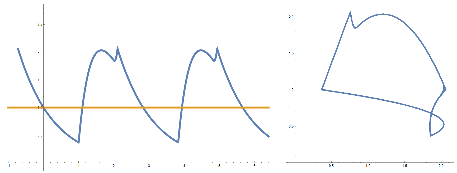
Figure 2: Plots of solution and their projection with the map $t\mapsto(p(t),p(t-1))$ in the case $k=2$ with parameter values $c=1$ and $d=7.38907)$.

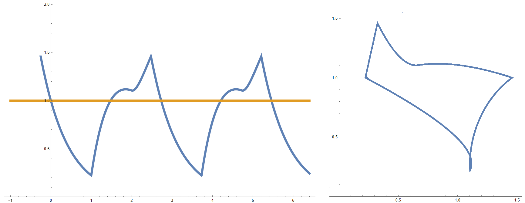
Figure 3: Plots of solution and their projection with the map $t\mapsto(p(t),p(t-1))$ in the case $k=\frac{1}{2}$ with parameter values $c=1.5$, and $d=3.1756$.

5 Property (P): computer assisted proofs

We assume the reader is familiar with work [2]. In what follows, similar to the aforementioned work, we will develop a method to prove, for a fixed $g$ and given parameters $c,d$ that the equation ($E_{g}$) has a periodic orbit as in the condition (P). The method from [2] would not work for functions $g$ used in this paper, therefore we use a general purpose algorithm for integration forward in time of DDEs from papers [42], [43]. The method is general in the sense that any form of $g$ given in terms of simple functions (composition of arithmetic operators and some analytic functions) can be used. We present examples for $g$ obtained as a limit $n\to\infty$ from our prototype nonlinearity (1.2) with $k=2$ and $k=1/2$.

Since ($E_{g}$) is discontinuous, the direct application of the algorithm from [43] is not possible and we adopt a technique similar to that of [2] to generate the segments of the solution that are smooth on explicitly given intervals. In short, we are computing images of the constitutive Poincaré maps to sections $S_{0}=\{\phi\in C([-1,0],\mathbb{R}^{+}):x(0)=1\}$ and $S_{1}=\{\phi\in C([-1,0],\mathbb{R}^{+}):x(-1)=1\}$. The algorithm from [43] will take care of providing the rigorous estimates on the solutions, crossing times and the transversality of the intersection with the section.

We would like to acknowledge that any algorithm that can continue solutions of DDEs forward in time can be used, as long as it can (a) do rigorous method of steps over full delay intervals and (b) it can compute intersection of the solutions with the sections $S_{0}$ and $S_{1}$. Several alternatives exists in the literature: [6, 26, 38]. The advantage of using [43] is that it provides Poincaré maps (point (b)) without additional effort and it is relatively easy to obtain estimates on segments $x_{t}$ of the solution without the assumption that $t$ is a multiple of the time lag.

We use the following notions from [2]. By $\mathbb{IR}$ we denote the set of all closed intervals in $\mathbb{R}$. Let $\phi:D\to\mathbb{R}$ and $[\alpha,\beta]\subset D$. Then:

$$\phi_{[\alpha,\beta]}:[0,\beta-\alpha]\to\mathbb{R} \quad\quad\phi_{[\alpha,\beta]}(s):=\phi(\alpha+s)$$

$$\phi_{[\alpha,\beta)}:[0,\beta-\alpha)\to\mathbb{R} \quad\quad\phi_{[\alpha,\beta)}(s):=\phi(\alpha+s)$$

We define the following spaces:

$$C^{>1}([0,\delta]) =\left\{\phi\in C([0,\delta],[1,\infty)):\forall_{s\in(0,\delta)}\ \phi(s)>1\right\},$$

$$C^{\leq 1}([0,\delta]) =C^{\infty}([0,\delta],[0,1]),$$

$$C^{+}_{seg}([0,\delta]) =C^{>1}([0,\delta])\cup C^{\leq 1}([0,\delta]),$$

$$C^{+}_{r,sol} =\left\{\phi\in C^{+}_{r}:\exists\{d_{i}\}_{i=0}^{m}\subset[-1,0],-1=d_{0}<\ldots<d_{m}=0,\right.$$

$$\left.\textrm{\quad\ \ and }\phi_{[d_{i},d_{i+1}]}\in C_{seg}([0,d_{i+1}-d_{i}])\textrm{ for all }0\leq i<m\right\}.$$

Here, instead of spaces $C^{\leq 1}_{pol}$ and $C^{+}_{r,comp}$ from [2], we will use $C^{\infty}([0,\delta],[0,1])$ and $C^{+}_{r,sol}$, respectively. It is clear that $C^{\leq 1}_{pol}\subset C^{\infty}([0,\delta],[0,1])$ and a similar fact to Lemma 4.3 from [2] can be stated:

Lemma 5.1.

Assume $g$ in ($E_{g}$) is of class $C^{\infty}$ with $g(\xi)\geq 0$ for $\xi\geq 0$. Let $\phi\in C^{+}_{r,sol}$ and $l\in(-1,0]$ be such that $\psi_{[-1,l]}\in C^{+}_{seg}$. Then, $x^{\phi}_{[0,l+1]}\in C^{\infty}([0,l+1],\mathbb{R}^{+})$.

Proof.

Either (a) $\phi_{[-1,l]}\in C^{>1}$ and, in that case, $x^{\phi}(s)=x(0)e^{-cs}$ for $s\in[0,l+1]$, or (b) $\phi_{[-1,l]}\in C^{\leq 1}$ and then $x^{\phi}|_{[0,l+1]}$ is a solution to a smooth ($C^{\infty}$) non-autonomous ODE $x^{\prime}(t)=-cx(t)+dh(t)$, with $h(t)=(g\circ\phi)(t)>0$. It has a solution

$$x^{\phi}(t)=e^{-ct}\phi(0)+d\int_{0}^{t}e^{s-t}h(s)ds\geq 0\qquad t\in[0,l+1]$$ (5.1)

∎

The two key features of Lemma 4.3 in [2] was that (a) it provided explicit formulas for $x^{\phi}_{[0,l+1]}$ and (b) it guaranteed that $x^{\phi}_{[0,l+1]}$ had finite number of intersections with the line $x=1$. This guaranteed that $\Gamma(1,\phi)\in C^{+}_{r,comp}$ for all $\phi\in C^{+}_{r,comp}$. It was possible because $h(s)$ in (5.1) was amenable to almost symbolic computations and the solutions were in the form of an exponential-polynomial products. In the current work we need to circumvent two problems: first, of an arbitrarily complicated $h(s)$ caused by a general representation of $C^{\infty}$ solution segment $\phi$ and second, we cannot prove a priori $\Gamma(1,\phi)\in C^{+}_{r,sol}$, as we do not explicitly know the number of intersections. Instead, our algorithm will prove along the way that $x_{[k,k+1]}\in C^{+}_{r,sol}$ for $k\in\{0,1,\ldots,K\}$ for a given $x_{[-1,0]}\in C^{+}_{r,sol}$. To do this, we need to introduce basic notions of the rigorous integration procedure from [43]. This algorithm works with the piecewise Taylor representation of solution segments. Let $\phi$ be some $C^{n+1}$ function, $\phi:[t,t+\delta)\to\mathbb{R}$. The forward jet of $\phi$ at $t$ is:

$$\left(J^{[n]}_{t}\phi\right)(s)=\sum_{k=0}^{n}\phi^{[k]}(t)s^{k}\quad s\in[t,t+s),$$

where $\phi^{[k]}(t)=\frac{\phi^{(k)}(t)}{k!}$ are coefficients of Taylor expansion of $\phi$. We identify the jet with a vector in $\mathbb{R}^{n+1}$ in a standard way: $J^{[n]}_{t}\phi\equiv\left(\phi^{[0]}(t),\ldots,\phi^{[n]}(t)\right)\in\mathbb{R}^{n+1}$. This allows to write $J^{[n]}_{t}\phi\in A\subset\mathbb{R}^{n+1}$, and we will use that frequently.

Definition 1.

The forward Taylor representation of $\phi:[t,t+\delta)$ is the pair

$$(J^{[n]}_{t}\phi,\xi)\subset\mathbb{R}^{n+1}\times C^{0}([t,t+\delta],\mathbb{R})$$

such that the Taylor formula is valid for $g$:

$$\phi(s)=\left(J^{[n]}_{t}\phi\right)(s)+(n+1)\int_{t}^{\delta}\xi(s)(t-s)^{n}ds,\quad s\in[t,t+\delta)$$

Obviously, $\xi(s)=\phi^{[n+1]}(s)$, and that we are assuming $\phi^{[n+1]}(s)$ bounded over $[t,t+\delta)$. In what follows, we will identify any such $\phi$ with its representation $(J^{[n]}_{t}\phi,\xi)$, and we will write $\phi\equiv(J^{[n]}_{t}\phi,\xi)$. For a given vector $j\in\mathbb{R}^{n+1}$ and a function $\xi$ we identify $(j,\xi)$ with a function $\phi:[0,\delta)\to\mathbb{R}$ given by (1) with $J^{[n]}_{0}\phi=j$. The order $n$ is known from the context (the length of the vector $j$). We will write $(j,\xi)(t)$ to denote the evaluation $\phi(t)$.

Definition 2.

A grid of size $h_{p}=\frac{1}{p}$ over the base interval $[-1,0]$ is the set of points $\left(t_{i}\right)_{i=0}^{p}$ with $t_{i}=-ih$. We have $t_{p}=-1$ and $t_{0}=0$.

We will usually drop subscript $p$. In what follows the constant $h$ will always mean the grid step size $h_{p}$ and the variable $\varepsilon$ will be such that $0\leq\varepsilon<h$.

Definition 3.

For a vector $\eta=(n_{1},\ldots,n_{p})$ the space $C^{\eta}_{p}$ is defined as:

$$C^{\eta}_{p} = \left\{x:[-1,0]\to\mathbb{R}:\exists j_{i}\in\mathbb{R}^{n_{i}+1},\exists\xi_{i}\in C^{0}([0,h],\mathbb{R})\right.$$

$$\left.\textrm{ such that }x_{[t_{i},t_{i-1})}\equiv(j_{i},\xi_{i})\right\}$$

Please note that functions in $C^{\eta}_{p}$ can be discontinuous at the grid points $t_{i}$. However, if the function $x$ is $C^{n+1}$-smooth on the whole $[-1,0]$, then obviously $x\in C^{n}_{p}$. Later, the discontinuities at the grid points will allow us to handle discontinuities arising from solving ($E_{g}$).

Definition 4.

A ($p$, $\eta$)-representation (or just the representation) of a function $x\in C^{\eta}_{p}$ is the collection of $(z,j_{1},\ldots,j_{p},\xi_{1},\ldots,\xi_{p})$, where $z=x(0)$ and $x_{[t_{i},t_{i-1}]}\equiv(j_{i},\xi_{i})$ as in Definition 3.

Please note, that $(z,j_{1},\ldots,j_{p},\xi_{1},\ldots,\xi_{p})=(z,j,\xi)$ can be think of as an element of $\mathbb{R}^{M}\times(C^{0}([0,h],\mathbb{R}))^{p}$ with additional structure (coefficients of $j$ divided among $p$-grid and $\eta$-orders). Here $M=M(p,\eta)=1+\sum_{j=1}^{p}(\eta_{i}+1)$. In the computations, the structure $\eta$ can be deduced from the structure of components of $j$. We will again just write that $x=(z,j,\xi)$ and we might write $(z,j,\xi)(t)$ to denote the evaluation of the corresponding $x$ at $t$. Note that if $t=-ih+\varepsilon$, then $(z,j,\xi)(t)=(j_{i},\xi_{i})(\varepsilon)$ and if $t=0$, then $(z,j,\xi)(t)=z$.

Now we need finite description of the subsets of $C^{\eta}_{p}$ to put them into computer. Let $Z,Y$ are closed intervals in $\mathbb{R}$ and $\xi\in C^{0}(Z,\mathbb{R})$. By writing $\xi\in Y$ we will denote the fact that $\left[\inf_{x\in Z}\xi(x),\sup_{x\in Z}\xi(x)\right]\subset Y$.

Definition 5.

The representable ($p$,$\eta$)-functions-set (or just f-set) is a pair

$$(A,\Xi)\subset\mathbb{R}^{M}\times\mathbb{IR}^{p}.$$

The support of the f-set is $X(A,\Xi)\subset C^{\eta}_{p}$:

$$x\in X(A,\Xi)\iff\exists(z,j)\in A,\exists\xi\in\Xi:x=(z,j,\xi).$$ (5.2)

We will often identify the f-set with its support. We will use projections: $z(A)$, $j(A)$, $j_{i}(A)$, to denote the respective components of the representation. For $x\in C^{\eta}_{p}$ by $X(x)$ we will denote the smallest f-set that contains the representation $(z,j,\xi)$ of $x$. If we want to stress out what ($p$, $\eta$)-representation we are using (e.g. when the space $C^{\eta}_{p}$ is not clear from the context), we will write $X^{\eta}_{p}(x)$. We use the convention that for $n\in\mathbb{N}$ $X^{n}_{p}=X^{\eta}_{p}$, with $\eta=(n,\ldots,n)$ - a uniform order over all grid points. We also note that it is easy, given an ($p$, $\eta$)-set $X$ with $\eta_{i}>0$ for all $i$, to obtain a ($p$, $\lambda$)-set $Y$ representing $\frac{dg}{dt}$ for all $g\in X$ (with $\lambda_{i}=\eta_{i}-1$). We will therefore write $X^{\prime}$ to denote this set. It will be used in Algorithm 2.

The work [43] provides two (families of) algorithms to propagate forward in time solutions to a general DDE of the form

$$x^{\prime}(t)=F\left(x(t),x(t-h),x(t-2h),\ldots,x(t-\tau)\right),$$ (5.3)

where $F$ is smooth enough. The algorithms are denoted by $\mathcal{I}:C^{\eta}_{p}\to C^{\lambda}_{p}$ and $\mathcal{I}^{\varepsilon}:C^{\eta}_{p}\to C^{\zeta}_{p}$, respectively, such that they guarantee for the semiflow $\varphi$ associated to DDE (5.3) the following:

• $\varphi(h,x)\in\mathcal{I}(X(A,\Xi))=X(B,\Lambda)\subset C^{\lambda}_{p}$, for all $x\in X(A,\Xi)$;

• $\varphi(\varepsilon,x)\in\mathcal{I}^{\varepsilon}(X(A,\Xi))=X(B,Z)\subset C^{\zeta}_{p}$ for all $x\in X(A,\Xi)$, such that $\varphi(\varepsilon,x)\in C^{\zeta}_{p}$.

• if $x\in X(A,\Xi)\cap C^{\infty}([-1,0],\mathbb{R})$, then it is guaranteed that $J^{[\zeta_{i}]}_{-ih}\varphi(\varepsilon,x)\in j_{i}(I_{\varepsilon}(X(A,\Xi)))$, for all $i\in 1,\ldots,p$.

The property (i) guarantees that the solution to any initial data in a ($p$,$\eta$)-fset are representable after full time step $h$. The properties (ii) and (iii) guarantees that, for solutions smooth enough, the shift by a step $\varepsilon$ smaller than the full step $h$ is well defined, and the shifted segment can be described by some ($p$,$\zeta$)-representation. The grid size $p$ of the representations must be the same, but the structure of the result sets given by $\lambda$ and $\zeta$ can be different from input $\eta$ for technical reasons, important to obtain rigorous results of good numerical quality. The details are given in [43], but Reader can think of $\mathcal{I}$ and $\mathcal{I}^{\varepsilon}$ just as functions $C^{\eta}_{p}\to C^{\eta}_{p}$, with a fixed $\eta$, for the sake of presentation of the methods. It is also easy to see that the iteration $\mathcal{I}^{p}$ realizes the classical method of steps for the DDEs, and a Poincaré map $P:S\supset D\to S$ might be realized as $\mathcal{I}^{[\varepsilon_{1},\varepsilon_{2}]}\circ\mathcal{I}^{m}$, if the return time function $t_{P}:S\supset D\to\mathbb{R}^{+}$ can be proved to be continuous and estimated by $t_{P}(D)\subset mh+[\varepsilon_{1},\varepsilon_{2}]$, $0\leq\varepsilon_{1}\leq\varepsilon_{2}<h$. The method from [43] can be used to prove that the Poincaré maps are well defined in that matter.

Definition 6.

Assume $p\in\mathbb{N}_{+}$ is the grid size.

The representation of a function $\phi\in C^{+}_{r,sol}$ is a collection of objects:

$$\left(z,\left((d_{i},z^{i},j^{i},\xi^{i})\right)_{i=0}^{m-1}\right)$$

such that $(z^{i},j^{i},\xi^{i})\in C^{\eta^{i}}_{p}$, $\phi_{[d_{i},d_{i+1}]}=(z^{i},j^{i},\xi^{i})_{[-1,-1+d_{i+1}-{d_{i}}]}$, and $z=\phi(0)$.

In other words, each ($p$,$\eta^{i}$)-representation $(z^{i},j^{i},\xi^{i})$ is given over whole basic interval, but we assume it is valid only on the initial segment of length $\delta_{i}=d_{i+1}-{d_{i}}$ (it might span several grid points, and the end point is not necessarily at the grid point, i.e. usually $\delta_{i}=k_{i}h+\varepsilon_{i}$, $k_{i}\in\mathbb{N}$, $\varepsilon_{i}\in[0,h)$). Each jet $j^{i}_{p}$ representing the function at $t=-ph=-1$ is matched with the jet of $\phi$ at time $d_{i}$, See Figure 4. The distinguished element $z$ is called the head of the solution (as in this analogue: the solution $x_{t}^{\phi}$ is a snake moving in the phase space, and the value $z$ represents $x_{t}^{\phi}(0)$ - its head - that is moving according to ($E_{g}$)). Analogously, we define f-set in $C^{+}_{r,sol}$ as a collection of f-sets:

$$\left(Z,\left((d_{i},A^{i},\Xi^{i})\right)_{i=0}^{m-1}\right).$$

The smallest f-set containing the representation of $\phi\in C^{+}_{r,sol}$ is denoted again as $X(\phi)$.

Figure 4: Schematic picture showing the representation of a function in $C^{+}_{r,sol}$ (d), build with $C^{n}_{p}$ representations (a-c). The dashed lines show parts of the $C^{n}_{p}$ representations not used in computations, while the coloured backgrounds show ranges of respective lengths $\delta_{i}=d_{i}-d_{i+1}$. In this case $i\in\{0,1,2\}$. In (d), the ranges are shown in respective colours between points $d_{i}$ and $d_{i+1}$, where the $C^{n}_{p}$ representation holds. The black dot in (d) is $z$ - the head of the representation.

Remark 2 (A technical note about the representation $\phi\in C^{+}_{r,sol}$).

It might be strange mathematically to represent $\phi$ by ,,gluing” together representations of $C^{\eta^{i}}_{p}$, especially, when there is a lot of unnecessary data, as each piece is valid only on (possibly) small interval $[-1,-1+\delta_{i})$. However, with such a representation we get a lot easier implementation of the algorithm to propagate data using the algorithms $\mathcal{I}$ and $\mathcal{I}^{\varepsilon}$, as the data is already in a good format.

We will now present Algorithm 1 to compute rigorous estimates on $x^{\phi}$ for $\phi=e^{-a(s+1)}$ over a long interval $[-1,M]$, $M\in\mathbb{N}$. The algorithm successively computes f-sets representing the solution as an element of $C^{+}_{r,sol}$ over consecutive intervals $[k-1,k]$, $k\in\mathbb{N}$. In what follows, we denote by $\mathcal{I}_{\leq 1}$, $\mathcal{I}^{\varepsilon}_{\leq 1}$, $\mathcal{I}_{>1}$, $\mathcal{I}^{\varepsilon}_{>1}$ the procedures from [43] that are configured to compute estimates on semiflows for smooth systems $x^{\prime}(t)=-ax(t)+bf(x(t-1))$ and $x^{\prime}(t)=-ax(t)$, respectively. To organize the presentation, we first give a very general description of Algorithm 1, then we shortly describe what the three subroutines used in it do, finally we state the main Lemma 5.2 about the correctness of the procedure. As the subroutines are very technical, their details are postponed to Appendix A, so is the proof of Lemma 5.2.

Algorithm 1 Main algorithm

1:$c,d$ - parameters of ($E_{g}$) and the f-set $X_{0}=X(\phi)\subset C^{+}_{r,sol}$

2:An f-set $X_{1}\subset C^{+}_{r,sol}$ such that it contains the solution $\Gamma(1,\phi)$ in the sense of Lemma 5.2.  

3:$U\leftarrow\texttt{shift}(X_{0})$ $\triangleright$ shift all subsegments by full time lag

4:$V\leftarrow\texttt{recut}(U)$ $\triangleright$ then, cut new segment at points crossing $x=1$

5:$X_{1}\leftarrow\texttt{rake}(V)$ $\triangleright$ finally, merge consecutive segments lying whole in $C^{>1}$.

6:return $X_{1}$

The additional procedures used in Algorithm 1 do the following:

• Algorithm 2 (Interval Newton’s Method) is a standard procedure to prove that there is a single zero of a function in a given neighbourhood. It can also be used to narrow the set to be as small as possible. We will use it as a sub-procedure in Algorithm 4 but we provide the pseudo-code for completeness and to demonstrate places where Algorithm 4 might fail later. What is more, the successful execution of the algorithm will guarantee that the Property (P2) is satisfied.

• Algorithm 3 - ,,shift”: realizes one iteration of the method of steps to convert $\phi$ into $\Gamma(1,\phi)$. The resulting description (pre-representation) is not a valid $C^{+}_{r,sol}$ f-set representation and it needs to be corrected for the subsequent iterations.

• Algorithm 4 - ,,re-cut”: makes sure to find all intersections of the pre-representation of $\Gamma(1,\phi)$ with the line $x=1$ and convert the pre-representation into representation in $C^{+}_{r,sol}$.

• Finally, Algorithm 5 - ,,rake”: removes all consecutive segments of the solution that lie in $C^{>1}$ and combines them into one segment. This reduces the size of the representation and in turn lessens the computational complexity of the subsequent steps. It also increases the accuracy, as the $\mathcal{I}_{>1}$ could be used for longer uninterrupted periods in Algorithm 3 resulting in less wrapping-effect impact of Line 13 in Algorithm 3.

Lemma 5.2.

Let $\phi\in C^{+}_{r,sol}$. If succeeds, Algorithm 1 applied to the f-set representation $X(\phi)$ produces an f-set $X=\left(Z,\left((\bar{d}_{i},A^{i},\Xi^{i})\right)_{i=0}^{m-1}\right)\subset C^{+}_{r,sol}$ with $\bar{d}_{i}\in\mathbb{IR}$ such that

1. if $d_{i}$ are the points where $\Gamma(1,\phi)(d_{i})=1$, then $d_{i}\in\bar{d}_{i}$,

2. if $\Gamma(1,\phi)_{[d_{i},d_{i+1}]}\in C^{\leq 1}$, then $\Gamma(1,\phi)_{[d_{i},d_{i+1}]}\in X_{[d_{i},d_{i+1}]}$.

Now we can state the results about the existence of periodic solutions to Eq. $E_{g}$ for concrete values of parameters. Before we do that however, we need to discuss shortly the floating-point arithmetics and its presentation in the article, following the convention used in [43]:

Remark 3 (On the representation of floating-point numbers from computations).

Due to the very nature of the implementation of real numbers in computers, numbers like $0.1$ are not representable [14], i.e. cannot be stored in the memory exactly. On the other hand, many representable numbers could not be shown in the text in a reasonable, human-readable way. As we use the interval arithmetic to produce rigorous estimates on the true values, whenever we present any output of the computer program $x$ as a decimal number with non-zero fraction part, then we have in mind that this in fact represents some other number $y$ such that $y\in B(x,\epsilon^{M})$, where $\epsilon^{M}$ is the machine precision of the double-precision floating point numbers as defined in [14]. This convention applies also to intervals: if we write an interval $[a_{1},a_{2}]$, then we understand this as $[b_{1},b_{2}]$ with $b_{1}$, $b_{2}$ - representable and such that $[a_{1},a_{2}]\subset[b_{1},b_{2}]$. Finally, if we write a number in the following manner: $d_{1}.d_{2}sd_{k}{}^{u_{1}u_{2}su_{m}}_{l_{1}l_{2}sl_{m}}$ with digits $l_{i},u_{i},d_{i}\in\{0,..,9\}$ then it represents the following interval

$$\left[d_{1}.d_{2}sd_{k}l_{1}l_{2}sl_{m},d_{1}.d_{2}sd_{k}u_{1}u_{2}su_{m}\right].$$

For example $12.3_{456}^{789}$ represents the interval $[12.3456,12.3789]$ (here we also understand the numbers taking into account the former conventions).

Now we present the result proven with the computer assistance:

Theorem 5.3.

For $k$, $c$, $d$, $T$, $\omega_{p}$ as in Table 1, the system ($E_{g}$) with $g(\xi)=\xi^{k}$ has a periodic orbit with the basic period $\omega_{p}$ satisfying (P).

Proof.

Let $\phi(s)=e^{-c(s+1)}$. We set $X_{0}=X(\phi)=X\left(\phi(0),\left(-1,X^{n}_{p}\left(\phi\right)\right)\right)$. Then we successively compute

$$X_{k}=\left(Z,\left(\bar{d}^{k}_{i},A^{k,i},\Xi^{k,i}\right)_{i=0}^{m_{k}-1}\right):=\mathtt{main}\left(X_{k-1}\right),\quad k\in 1,\ldots,T.$$ (5.4)

Note, the sets $\bar{d}^{k}_{i}\in\mathbb{IR}$ contains the true $d^{k}_{i}$’s, according to Lemma 5.2. Next, we show that there exists $\bar{d}^{T-1}_{m_{T-1}}$ and $\bar{d}^{T}_{1}$, such that:

1. $\omega_{p}\in T+1+\bar{d}^{T}_{1}\subset[T,T+1]$;

2. $1=x^{\phi}(\omega_{p}-1)\in(X_{T})(\bar{d}^{T}_{1})$;

3. $\bar{d}^{T-1}_{m_{T-1}}-\bar{d}^{T}_{1}\geq 0$;

4. $X(A^{T-1,m_{T-1}},\Xi^{T-1,m_{T-1}})\in C^{\geq 1}$ and $X(A^{T,0},\Xi^{T,0})\in C^{\geq 1}$.

Note, that all those conditions imply that $\Gamma(\omega_{p}-1,\phi)\in C^{\geq 1}$, and therefore $\Gamma(\omega_{p},\phi)=\phi$. Especially, $L=\bar{d}^{T-1}_{m_{T-1}}-\bar{d}^{T}_{1}+1$ is the length of the solution segment $x^{\phi}_{[\omega_{p}-1-L,\omega_{p}-1]}\geq 1$, so the condition C) imply $L>1$ and guarantees $\Gamma(\omega_{p},\phi)=\phi$. ∎

Parts of the proof are computer assisted: propagation of (5.4) and checking the four assumptions A-D. Programs to redo computations are available in [44]. Some of the orbits proved in Theorem 5.3 are shown in Figures 5 and 6, in particular we point out the last plot in Figure 5, as it shows a complicated periodic orbit $p$ for the values of parameters $k=2$, $c=5\pi/(3\sqrt{3})$, $d=7.95$ for which a Hopf bifurcation occurs near the equilibrium point $\frac{c}{d}$. In a future paper it will be shown that there is a heterocilinic connection to $p$ from a small amplitude periodic solution

Table 1: Values of parameters $k$, $c$, $d$ in ($E_{g}$), with $g|_{[0,1)}(\xi)=\xi^{k}$ and the estimated period $\omega_{p}$ of the periodic solutions. The parameters $T$, $n$, $p$ are as in the proof of Theorem 5.3, together with the estimated length $L$ of the last interval, over which the solution $x^{\phi}$ lies above line $x=1$. Presented values, when not computer-representable, are stored during the computations as intervals containing them as discussed in Remark 3. In particular, the value $c=5\cdot\pi/(3\cdot\sqrt{3})$ means that in computations the rigorous interval containing this value was used, and the proof is valid for all values of $c$ in that interval.

$k$	$c$	$d$	$T$	$p$	$n$	$\omega_{p}$	$L$
$2$	$2$	$20$	$3$	$128$	$4$	$2.2475762_{8868803}^{9130349}$	$1.19642835_{388474}^{650057}$
$2$	$2$	$5$	$10$	$128$	$4$	$9.718074_{41624915}^{68592668}$	$1.173666_{27746896}^{65610938}$
$2$	$5$	$13.5$	$11$	$128$	$4$	$10.3996_{6084251935}^{8118185736}$	$1.051_{39513368493}^{42163578326}$
$2$	$4$	$12.71$	$16$	$512$	$5$	$15.50313_{451849748}^{939964593}$	$1.1477_{3973007044}^{4713794320}$
$2$	$\frac{5\cdot\pi}{3\cdot\sqrt{3}}$	$7.95$	$15$	$256$	$4$	$14.70203_{302733336}^{563332337}$	$1.10426_{444733693}^{787605344}$
$\frac{1}{2}$	$2.5$	$5.1$	$9$	$128$	$4$	$8.714_{57545370406}^{62830383538}$	$1.154_{25881778764}^{36842629369}$
$\frac{1}{2}$	$2.5$	$5.2$	$12$	$256$	$5$	$11.4322_{6910337948}^{7232415869}$	$1.15709_{158785186}^{779182356}$
$\frac{1}{2}$	$3.8$	$5.205$	$17$	$1024$	$5$	$15.6237_{3745723471}^{4300377583}$	$1.0616_{4001088705}^{5181449065}$
$\frac{1}{2}$	$3.8$	$5.2$	$15$	$1024$	$5$	$13.741833_{36789089}^{66133022}$	$1.05535_{361584126}^{410986789}$
$\frac{1}{2}$	$3.8$	$5.195$	$15$	$1024$	$5$	$13.63633_{685525799}^{711062829}$	$1.054959_{16531613}^{80790828}$
$\frac{1}{2}$	$3.81$	$5.215$	$15$	$1024$	$5$	$13.743261_{57465981}^{86363402}$	$1.05439_{789658996}^{837966255}$
$\frac{1}{2}$	$4.65$	$6.51$	$16$	$1024$	$5$	$14.735_{51192774460}^{70287262517}$	$1.041_{71346771675}^{98571950225}$
$\frac{1}{2}$	$4.66$	$6.53$	$15$	$1024$	$5$	$14.730_{16163977130}^{21436894118}$	$1.047_{84259656712}^{96838456861}$

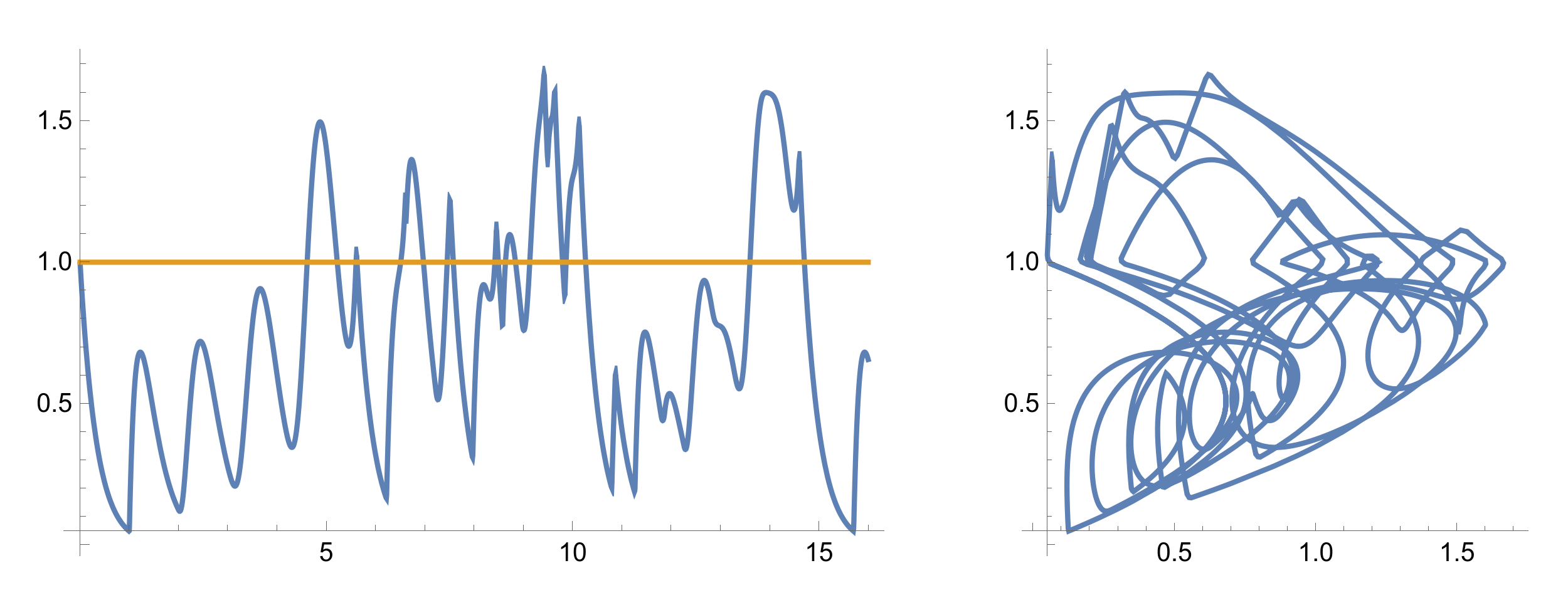
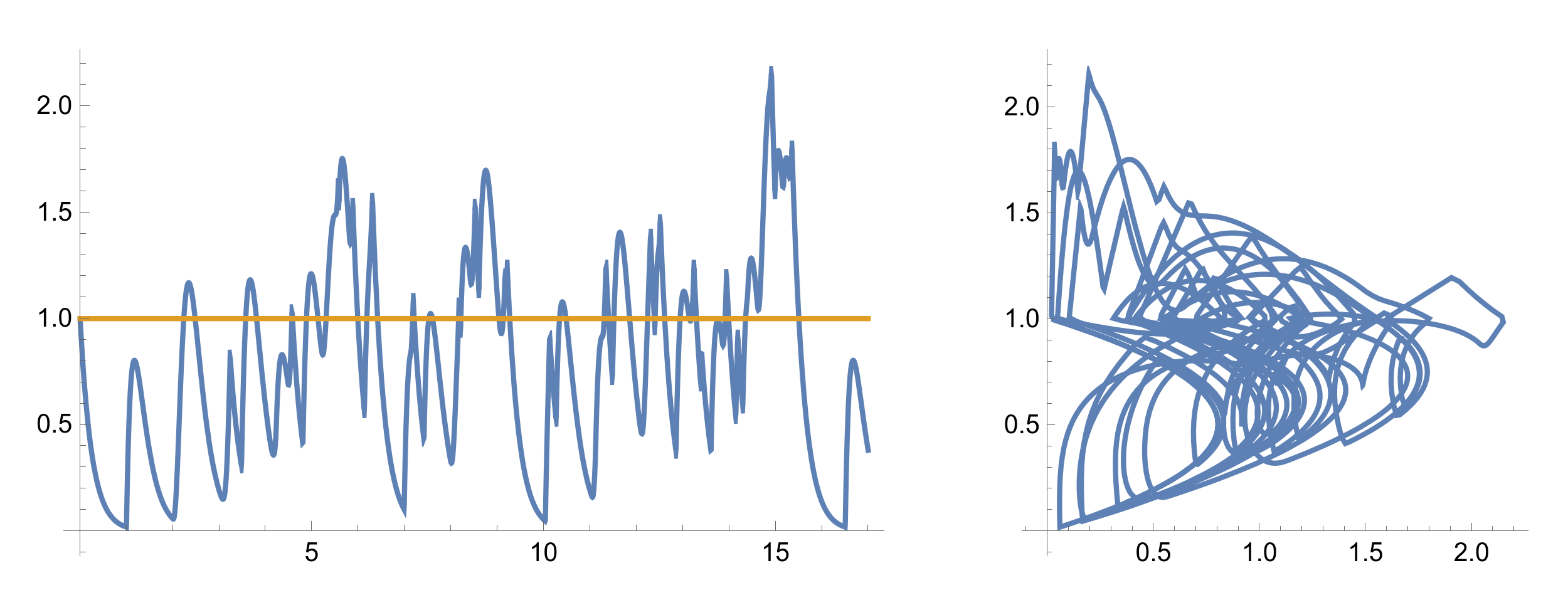
Figure 5: Plots of the numerical representations of solutions corresponding to entries in Table 1 for $k=2$, presented in the same fasion as in Figure 2. Solutions correspond to small intervals containing values of parameters: $c=\frac{5\cdot\pi}{3\cdot\sqrt{3}}$ (i.e. parameter of Hopf biffurcation at $\xi_{0}$), $d=7.95$ (up), and $c=4$, $d=12.71$ (bottom).

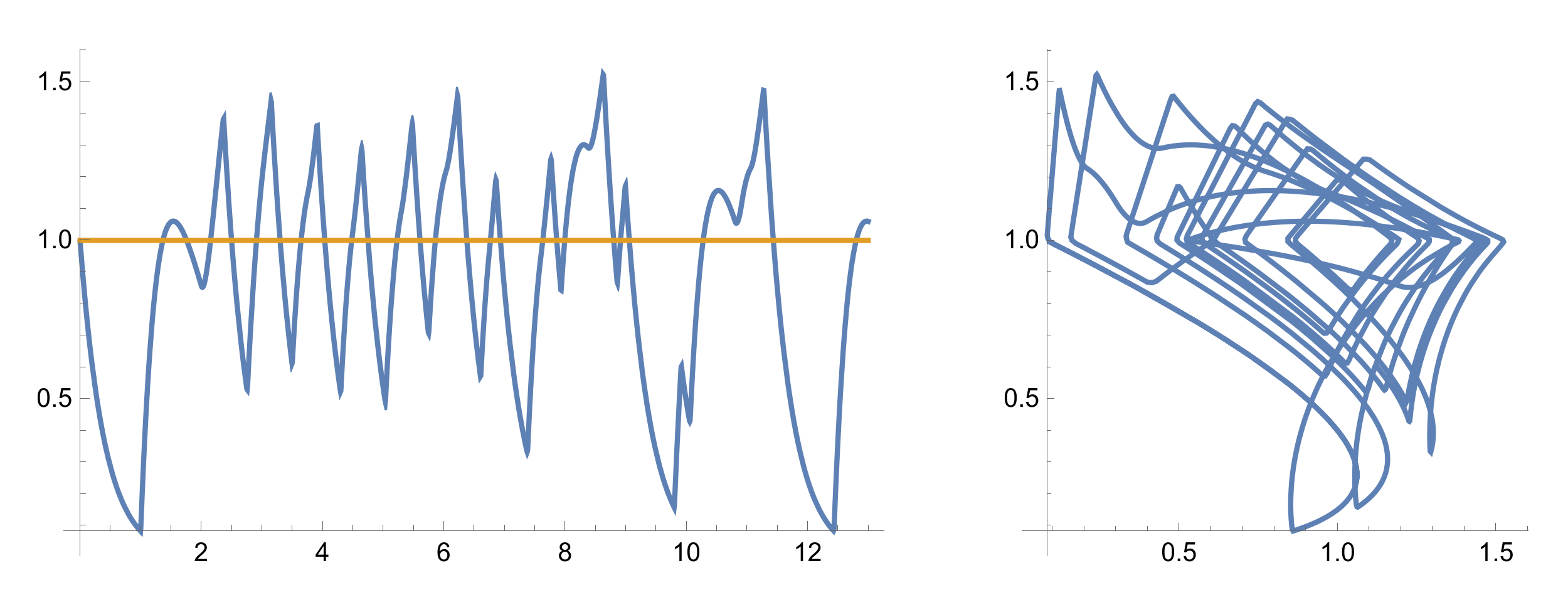
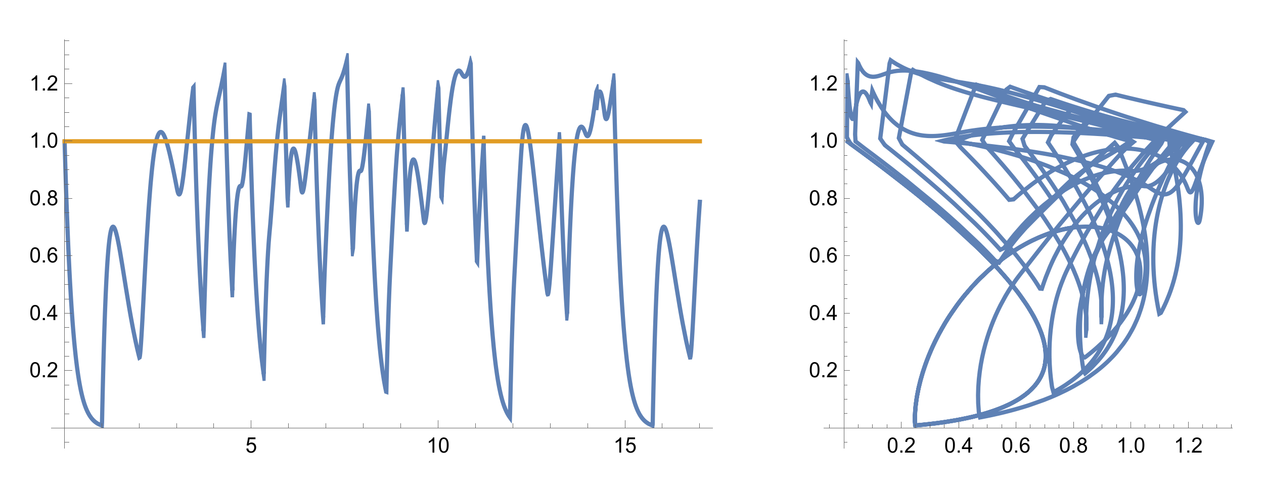
Figure 6: Plots of the numerical representations of solutions corresponding to entries in Table 1 for $k=1/2$, presented in the same fasion as in Figure 2. Solutions correspond to small intervals containing values of parameters: $c=2.5$, $d=5.2$ (up), and $c=4.65$, $d=6.51$ (bottom).

Appendix A Details on the algorithms

Algorithm 2 inewton: for a (forward) Taylor representation $(J,\Xi)$ of $f$ over $I=[0,\delta]$ proves either: 1) there is no root of $f$ in $I$, 2) there is exactly one root $t_{0}\in[0,\delta]$, or c) raises an error if multiple zeroes are possible. We use notation $[x]$ to denote a set $[x]\subset\mathbb{IR}$ such that it contains $x\in[x]$. Operations $\operatorname{\mathbf{diam}}([a,b]):=b-a$ and $\operatorname{\mathbf{mid}}([a,b]):=\frac{a+b}{2}$ denote the diameter and the middle point of the set, respectively.

1:$(J,\Xi)\subset\mathbb{R}^{n+1}\times\mathbb{IR}$, $I=[0,\delta]$, $\epsilon_{M}\in\mathbb{R}_{+}$, $M\in\mathbb{N}$.

2:$Z_{x}=\{t\in I:x(t)=a\}=\{t_{0}\}\subset\bar{t}_{0}\subset[0,\delta]$ or $Z_{x}=\emptyset$ for all $x=(j,\xi)\in(J,\Xi)$. It returns $\bar{t}_{0}\in\mathbb{IR}$.  

3:$(J^{\prime},\Xi^{\prime})\leftarrow\left((iJ_{i})_{i=1}^{n},(n+1)\Xi\right)$ $\triangleright$ representation of the derivative

4:$[t_{0}]=[0,\delta];\quad t_{0}=\frac{\delta}{2}$ $\triangleright$ choose $t_{0}\in\bar{t}_{0}$

5:$k=0$

6:while $k<M\land\operatorname{\mathbf{diam}}(t_{k})>\epsilon_{M}$ do $\triangleright$ common stop conditions

7:     if $[t_{k}]=\emptyset\lor a\notin(J,\Xi)([t_{k}])$ then $\triangleright$ there is no chance for solution in $I$

8:         return $\emptyset$

9:     end if

10:     if $0\in(J,\Xi)^{\prime}([t_{k}])$ then $\triangleright$ Newton’s operator ill-defined

11:         Raise an Error and Abort

12:     end if

13:     $[t_{k+1}]=\left(t_{k}-\frac{(J,\Xi)(t_{k})-a}{(J,\Xi)^{\prime}([t_{k}])}\right)\cap[t_{k}]\quad t_{k+1}=\operatorname{\mathbf{mid}}([t_{k+1}])$

14:     $k\leftarrow k+1$

15:end while

16:if $t_{k}\subset\operatorname{\mathbf{int}}(t_{0})$ then $\triangleright$ one need strong inclusion to prove uniqueness

17:     return $t_{k}$

18:else

19:     Raise an Error and Abort

20:end if

Algorithm 3 shift: computes a segment after one full delay

1:$X(W)\subset C^{+}_{r,sol}$, $W=\left(Z,(d_{i},A^{i},\Xi^{i})_{i=0}^{m-1}\right)$ for some $m\in\mathbb{N}_{+}$.

2:$\left(Z^{\prime},\left(d_{i},A^{\prime i},\Xi^{\prime i}\right)_{i=0}^{m-1}\right)$ such that $\Gamma(1,x)(0)\in Z^{\prime}$ and $\Gamma(1,x)_{[d_{i},d_{i+1}]}=y_{[-1,-1+\delta_{i}]}$ for some $y\in X(A^{\prime i},\Xi^{\prime i})\subset C^{\eta^{\prime}_{i}}_{p}$, for all $x\in X(W)$.  

3:$head\leftarrow Z$ $\triangleright$ start at the current value of the solution

4:for $i=0$ to $m-1$  do $\triangleright$ then process all subsequent segments

5:     $\tilde{A}\leftarrow\left(head,j(A^{i})\right)$ $\triangleright$ change segment head to the correct value

6:     if $(\tilde{A},\Xi^{i})_{[-1,-1+\delta_{i}]}\subset C^{>1}$ then

7:         $(A^{\prime i},\Xi^{\prime i})=\mathcal{I}_{>1}^{p}\left(\tilde{A},\Xi^{i}\right)$ $\triangleright$ Propagate with the correct part of ($E_{g}$)

8:     else if $(\tilde{A},\Xi^{i})_{[-1,-1+\delta_{i}]}\subset C^{\leq 1}$ then

9:         $(A^{\prime i},\Xi^{\prime i})=\mathcal{I}_{\leq 1}^{p}\left(\tilde{A},\Xi^{i}\right)$ $\triangleright$ Propagate with the correct part of ($E_{g}$)

10:     else

11:         Raise an Error and Abort $\triangleright$ Should not happen for a correct $X(W)$

12:     end if

13:     $head\leftarrow\left(A^{\prime i},\Xi^{\prime i}\right)(-1+\delta_{i})$ $\triangleright$ update the head to the current value

14:end for

15:$Z^{\prime}\leftarrow head$ $\triangleright$ the new head of the whole solution is the last head

16:if $1\in Z^{\prime}$ then $\triangleright$ this would break the subsequent call to shift!

17:     Raise an Error and Abort

18:end if

19:return $\left(Z^{\prime},(d_{i},A^{\prime i},\Xi^{\prime i})_{i=0}^{m-1}\right)$

Algorithm 4 recut: computes intersections with $x=1$ and reorganizes the $C^{+}_{r,sol}$ representation accordingly

1:$W=\left(Z,(d_{i},A^{i},\Xi^{i})_{i=0}^{m-1}\right)$ as in the output of Algorithm 3.

2:$W^{\prime}=\left(Z,(d^{\prime}_{i},A^{\prime i},\Xi^{\prime i})_{i=0}^{m^{\prime}-1}\right)$ such that $W\subset C^{+}_{r,sol}$ and $X(W)\subset X(W^{\prime})$, $m^{\prime}\geq m$.  

3:for all $(d_{i},A^{i},\Xi^{i})$ do

4:     $T=$ empty list

5:     for all $k\in\mathbb{N}:-kh\in[-1,-1+\delta_{i}]$ do

6:         $(\varepsilon_{k},sign)=\mathtt{inewton}\left((A^{i}_{k},\Xi^{i}_{k}),a=1,\epsilon_{M}=10^{-15},M=10\right)$

7:         if $\varepsilon_{k}\neq\emptyset$ then $\triangleright$ $\varepsilon_{k}$ is the ,,local time” within $[-kh,-kh+1]$

8:              add $(k,\varepsilon_{k})$ to the end of $T$ $\triangleright$ we add global time $kh+\varepsilon$

9:         end if

10:     end for

11:     $(\tilde{A},\tilde{\Xi})\leftarrow(A^{i},\Xi^{i})$;  $\tilde{t}\leftarrow d_{i}$

12:     if $(\tilde{A},\tilde{\Xi})$ was computed with $\mathcal{I}^{p}_{\leq 1}$ then $\triangleright$ choose the right $\mathcal{I}$ algorithm

13:         $\left(\tilde{\mathcal{I}},\tilde{\mathcal{I}}^{\varepsilon}\right)=\left(\mathcal{I}_{\leq 1},\mathcal{I}^{\varepsilon}_{\leq 1}\right)$

14:     else if $(\tilde{A},\tilde{\Xi})$ was computed with $\mathcal{I}^{p}_{>1}$ then

15:         $\left(\tilde{\mathcal{I}},\tilde{\mathcal{I}}^{\varepsilon}\right)=\left(\mathcal{I}_{>1},\mathcal{I}^{\varepsilon}_{>1}\right)$

16:     else$\triangleright$ should not happen

17:         Raise an Error and Abort

18:     end if

19:     $(\tilde{A},\tilde{\Xi})\leftarrow(A^{i},\Xi^{i})$;  $\tilde{t}\leftarrow d_{i}$

20:     for all $(k,\varepsilon)\in T$ do

21:         Add $(\tilde{t},\tilde{A},\tilde{\Xi})$ to the output

22:         $(\tilde{A},\tilde{\Xi})\leftarrow\left(\tilde{\mathcal{I}}^{\varepsilon}\circ\tilde{\mathcal{I}}_{\leq 1}^{k}\right)(A^{i},\Xi^{i})$ $\triangleright$ always start from initial!

23:         $\tilde{t}\leftarrow d_{i}+kh+\varepsilon$

24:     end for

25:     Add $(\tilde{t},\tilde{A},\tilde{\Xi})$ to the output

26:end for

Algorithm 5 rake: removes redundant segments in $C^{>1}$

1:$W=\left(Z,(d_{i},A^{i},\Xi^{i})_{i=0}^{m-1}\right)\subset C^{+}_{r,sol}$ (as in output of

2:$W^{\prime}=\left(Z,(d^{\prime}_{i},A^{\prime i},\Xi^{\prime i})_{i=0}^{m^{\prime}-1}\right)\subset C^{+}_{r,sol}$ such that $F\left(1,X(W)\right)=F\left(1,X(W)\right)$ and $m^{\prime}\leq m$.  

3:$i\leftarrow 0$, $m^{\prime}\leftarrow 0$

4:$d^{\prime}_{0}\leftarrow d_{0}$

5:$d^{\prime}_{1}\leftarrow d_{1}$

6:while $i<m-1$ do

7:     $(A^{\prime K},\Xi^{\prime K})\leftarrow(A^{i},\Xi^{i})$

8:     $j\leftarrow i+1$

9:     if $(A^{i},\Xi^{i})_{[-1,-1+\delta_{i}]}\in C^{>1}$ then $\triangleright$ if true, check following intervals

10:         while $j<m-1\land(A^{j},\Xi^{j})_{[-1,-1+\delta_{j}]}\subset C^{>1}$ do

11:              $d^{\prime}_{m^{\prime}+1}=d_{j+1}$ $\triangleright$ make the current interval to cover also $[d_{j},d_{j+1}]$

12:              $j\leftarrow j+1$ $\triangleright$ next, try another segment

13:         end while

14:     end if

15:     $i\leftarrow j$ $\triangleright$ we have skipped all previous intervals

16:     $m^{\prime}\leftarrow m^{\prime}+1$

17:end while

18:return $\left(Z,\left(d^{\prime}_{i},A^{\prime i},\Xi^{\prime i}\right)_{i=0}^{m^{\prime}-1}\right)$

Proof of Lemma 5.2.

Correctness of Algorithm 2 is well known, see e.g. [17] and references therein, and it produces $\bar{d}_{i}$ as in A). Algorithm 3 produces rigorous estimates following the correctness of the algorithm $\mathcal{I}$ of [43] to propagate any $C^{\eta}_{p}$ f-sets. Algorithm 4 works for all solutions such that their segment is smooth enough. Lemma 5.1 ensures that for a segment $\phi_{[d_{i},d_{i+1}]}\in C^{\infty}$ the solution $F\left(1,\phi_{[d_{i},d_{i+1}]}\right)$ (appearing in the output of Algorithm 3 and as an input to Algorithm 4) must also be $C^{\infty}$, so applying $\mathcal{I}_{\varepsilon}$ is justified. Algorithm 5 modifies the solution segment only in the sub-segments that lie in $C^{\geq 1}$, thus not altering the ,,important parts” shown in B). ∎

Remark 4 (Data stored in the algorithms).

We use $\delta_{i}=d_{i+1}-{d_{i}}>0$, to denote the length of the ,,definition” intervals in space $C^{+}_{r,sol}$. In the actual implementation [44], we store $\delta_{i}$’s instead of $d_{i}$’s, and recompute $d_{i}$ when needed, using the fact that $d_{0}=-1$.

References

- [1] B. Bánhelyi, T. Csendes, T. Krisztin, A. Neumaier, Global attractivity of the zero solution for Wright’s equation. SIAM J. Appl. Dyn. Syst. 13 (2014), 537-563.
- [2] Ferenc A Bartha, Tibor Krisztin, Alexandra Vígh, Stable periodic orbits for the Mackey-Glass equation, Journal of Differential Equations, 296 (2021), 15-49.
- [3] S. Beretka, G. Vas, Saddle-node bifurcation of periodic orbits for a delay differential equation, J. Differential Equations 269 (2020), 4215-4252.
- [4] Leonid Berezansky, Elena Braverman, Lev Idels, Mackey-Glass model of hematopoiesis with non-monotone feedback: Stability, oscillation and control, Applied Mathematics and Computation, Volume 219, Issue 11, (2013).
- [5] J.B. van den Berg, J. Jaquette, A proof of Wright’s conjecture. J. Differential Equations 264 (2018), no. 12, 7412-7462.
- [6] K.E.M. Church, Validated integration of differential equations with state-dependent delay, Communications in Nonlinear Science and Numerical Simulation, 115:106762, (2022).
- [7] V. Duruisseaux and A.R. Humphries, Bistability, bifurcations and chaos in the Mackey–Glass equation, Journal of Computational Dynamics, 9 (2022), 421–450.
- [8] O. Diekmann, S. M. Verduyn Lunel, S. A. van Gils and H.-O. Walther, Delay Equations. Functional-, Complex-, and Nonlinear Analysis, Springer-Verlag, New York, (1995).
- [9] D. Franco, C. Guiver, J. Perán, On the global attractor of delay differential equations with unimodal feedback not satisfying the negative Schwarzian derivative condition, Electron. J. Qual. Theory Differ. Equ. 2020, No. 76, 1-15.
- [10] Jianfang Gao, Fuyi Song, Oscillation analysis of numerical solutions for nonlinear delay differential equations of hematopoiesis with unimodal production rate, Applied Mathematics and Computation, Volume 264, Pages 72-84, (2015).
- [11] P. Hao, X. Wang and J. Wei, Global Hopf bifurcation of a population model with stage structure and strong Allee effect, Discrete and Continuous Dynamical Systems S, 10 (2017), 973–993.
- [12] U. an der Heiden, H.-O. Walther, Existence of chaos in control systems with delayed feedback, J. Differential Equations 47 (1983), 273-295.
- [13] C. Huang,Z. Yang, T. Yi and X. Zou, On the basins of attraction for a class of delay differential equations with non-monotone bistable nonlinearities, J. Differential Equations, 256(2014), 2101–2114.
- [14] IEEE Computer Society, IEEE Standard for Floating-Point Arithmetic, published online: http://ieeexplore.ieee.org/servlet/opac?punumber=4610933, DOI: doi:10.1109/IEEESTD.2008.4610935, ISBN 978-0-7381-5753-5, (2008), Accessed: 2022-06-24.
- [15] V. Ignatenko, Homoclinic and stable periodic solutions for differential delay equations from physiology. Discrete Cont. Dynamical Syst. 38 (2018), 3637-3661.
- [16] J. Jaquette, J.P. Lessard, K. Mischaikow, Stability and uniqueness of slowly oscillating periodic solutions to Wright’s equation. arXiv:1705.02432v1[math:DS], (2017).
- [17] R. Krawczyk and A. Neumaier, An improved interval newton operator, Journal of Mathematical Analysis and Applications, 118(1):194–207, (1986).
- [18] T. Krisztin, Global dynamics of delay differential equations. Period. Math. Hungar. 56 (2008), 83-95.
- [19] T. Krisztin, M. Polner, G. Vas, Periodic solutions and hydra effect for delay differential equations with nonincreasing feedback, Qual. Theory Dyn. Syst. 16 (2017), 269-292.
- [20] T. Krisztin, G. Vas, Large-amplitude periodic solutions for differential equations with delayed monotone positive feedback. J. Dynam. Differential Equations 23 (2011), 727-790.
- [21] T. Krisztin, G. Vas, The unstable set of a periodic orbit for delayed positive feedback. J. Dynam. Differential Equations 28 (2016), 805-855.
- [22] T. Krisztin, H.-O. Walther, Unique periodic orbits for delayed positive feedback and the global attractor. J. Dynam. Differential Equations 13 (2001), 1-57.
- [23] T. Krisztin, H.-O. Walther, Jianhong Wu, Shape, Smoothness and Invariant Stratification of an Attracting Set for Delayed Monotone Positive Feedback, Fields Institute Monographs, Vol. 11, Amer. Math. Soc., Providence, RI, (1999).
- [24] Yang Kuang, Delay Differential Equations With Applications in Population Dynamics, Mathematics in Science and Engineering Book series, Volume 191, Pages iii-xii, 3-398 (1993)
- [25] A. Lasota and M. Wazewska-Czyzewska, Matematyczne problemy dynamiki ukladu krwinek czerwonych (Polish) [Mathematical problems of the dynamics of red blood cell population], Matematyka Stosowana, vi (1976), 23-40.
- [26] J-P. Lessard and J.D. Mireles James. A rigorous implicit Chebyshev integrator for delay equations, Journal of Dynamics and Differential Equations, 33:1959-1988, (2021).
- [27] Lin, G., Lin, W., and Yu J. Basins of attraction and paired Hopf bifurcations for delay differential equations with bistable nonlinearity and delay-dependent coefficient, Journal of Differential Equations, Vol. 354 (2023), pp 183-206
- [28] E. Liz and A. Ruiz-Herrera, Delayed population models with Allee effects and exploitation, Mathematical Biosciences ans Engineering, 12 (2015), 83-97.
- [29] E. Liz and G. Röst, Dichotomy results for delay differential equations with negative Schwarzian derivative, Nonlinear Analysis: Real World Applications, Vol. 11 (2010), 1422-1430.
- [30] E. Liz and G. Röst, On the global attractor of delay differential equations with unimodal feedback, Discrete and Continuous Dynamical Systems 24 (2009), 1215-1224.
- [31] M. Mackey and L. Glass, Oscillation and chaos in physiological control systems, Science, New Series, (197) (1977), 286-289.
- [32] M.C. Mackey, C. Ou, L. Pujo-Menjeout and J. Wu, Periodic oscillations of blood cell population in chronic myelogenous leukemia, SIAM J. Math. Anal. 38 (2006), 166-187.
- [33] J. Mallet-Paret, G.R. Sell, The Poincaré-Bendixson theorem for monotone cyclic feedback systems with delay. J. Differential Equations 125 (1996), no. 2, 441-489.
- [34] A. Matsumoto, F. Szidarovszky, Asymptotic behavior of a delay differential neoclassical growth model, Sustainability 5 (2013), 440-455; doi:10.3390/su5020440
- [35] A. Yu. Morozov, M. Banerjee, S. V. Petrovskii Long-term transients and complex dynamics of a stage-structured population with time delay and the Allee effect, Journal of Theoretical Biology, Volume 396, (2016), Pages 116-124
- [36] C. Ou, J Wu, Periodic solutions of delay differential equations with a small parameter: existence, stability and asymptotic expansion, J. Dynam. Differential Equations 16 (2004), 605-628.
- [37] G. Röst and J. Wu, Domain-decomposition method for the global dynamics of delay differential equations with unimodal feedback, Proc. R. Soc. A, 463 (2007), 2655-2669.
- [38] A. Rauh and E. Auer. Verified integration of differential equations with discrete delay, Acta Cybernetica, 25(3):677-702, (2022).
- [39] Ruan, S., Delay differential equations in single species dynamics, Delay Differential Equations and Applications. NATO Science Series, vol 205. Springer, (2006)
- [40] A. Skubachevskii, H.-O. Walther, On the Floquet multipliers of periodic solutions to nonlinear functional differential equations, J. Dyn. Di er. Equ. 18 (2006), 257-355.
- [41] Hal Smith, An Introduction to Delay Differential Equations with Applications to the Life Sciences, Texts in Applied Mathematics (TAM, volume 57), (2011)
- [42] Robert Szczelina, P. Zgliczyński, Algorithm for Rigorous Integration of Delay Differential Equations and the Computer-Assisted Proof of Periodic Orbits in the Mackey-Glass Equation, Found. Comput. Math., (2017). DOI: 10.1007/s10208-017-9369-5
- [43] Szczelina, R., Zgliczyński, P. High-Order Lohner-Type Algorithm for Rigorous Computation of Poincaré Maps in Systems of Delay Differential Equations with Several Delays. Found Comput Math (2023). https://doi.org/10.1007/s10208-023-09614-x
- [44] R. Szczelina, Source codes for this article http://scirsc.org/p/piecewise-dde/, Accessed: 2023-17-07.
- [45] G. Vas, Configurations of periodic orbits for equations with delayed positive feedback. J. Differential Equations 262 (2017), 1850-1896.
- [46] H.-O. Walther, Contracting return maps for some delay differential equations. In: Faria, T., Freitas, P. (eds.) Topics in Functional Differential and Difference Equations. Fields Institute Communications Series, vol. 29, pp. 349-360. AMS, Providence (2001).
- [47] H.-O. Walther, Contracting return maps for monotone delayed feedback, Discrete Contin. Dyn. Syst. 7 (2001), 259-274.
- [48] B. Lani-Wayda, Change of the attractor structure for when changes from monotone to non-monotone negative feedback, J. Differential Equations, 248 (2010), 1120-1142.
- [49] B. Lani-Wayda, Erratic solutions of simple delay equations. Trans. Amer. Math. Soc. 351 (1999), no. 3, 901-945.
- [50] B. Lani-Wayda, Wandering solutions of delay equations with sine-like feedback. Mem. Amer. Math. Soc. 151 (2001), no. 718, x+121 pp.
- [51] B. Lani-Wayda, H.-O. Walther, Chaotic motion generated by delayed negative feedback.I. A transversality criterion. Differential Integral Equations 8 (1995), no. 6, 1407-1452.
- [52] B. Lani-Wayda, H.-O. Walther, Chaotic motion generated by delayed negative feedback. II. Construction of nonlinearities. Math. Nachr. 180 (1996), 141-211.
- [53] H.-O.Walther, The impact on mathematics of the paper - Oscillation and Chaos in Physiological Control Systems" by Mackey and Glass in Science, 1977, (2020), Eprint, arXiv:2001.09010
- [54] J. Wei, Bifurcation analysis in a scalar delay differential equation, Nonlinearity 20 (2007), 2483-2498.
- [55] E.M. Wright, A nonlinear difference-differential equation. J. Reine Angew. Math. 194 (1955), 66-87.