The Existential Theory of the Reals as a Complexity Class: A Compendium

Abstract

We survey the complexity class $\exists\mathbb{R}$, which captures the complexity of deciding the existential theory of the reals. The class $\exists\mathbb{R}$ has roots in two different traditions, one based on the Blum-Shub-Smale model of real computation, and the other following work by Mnëv and Shor on the universality of realization spaces of oriented matroids. Over the years the number of problems for which $\exists\mathbb{R}$ rather than  has turned out to be the proper way of measuring their complexity has grown, particularly in the fields of computational geometry, graph drawing, game theory, and some areas in logic and algebra. $\exists\mathbb{R}$ has also started appearing in the context of machine learning, Markov decision processes, and probabilistic reasoning.

We have aimed at collecting a comprehensive compendium of problems complete and hard for $\exists\mathbb{R}$, as well as a long list of open problems. The compendium is presented in the third part of our survey; a tour through the compendium and the areas it touches on makes up the second part. The first part introduces the reader to the existential theory of the reals as a complexity class, discussing its history, motivation and prospects as well as some technical aspects.

Keywords: existential theory of the reals, $\exists\mathbb{R}$, stretchability, Mnëv, Shor, universality, computational complexity.

Introduction

How many guards are necessary to guard an art gallery—a simple polygon on $n$ vertices—if every location inside the gallery must be seen by at least one of the guards? Chvátal [C75b] famously proved that at most $n/3$ guards are needed and that this bound is tight in general.

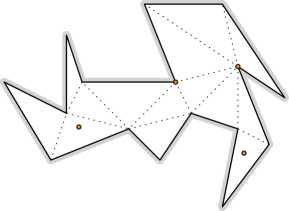
Figure 1: A gallery with $16$ vertices that can be guarded with $4<\lfloor 16/3\rfloor$ guards.

Figure 1 shows that for specific layouts fewer than $n/3$ guards may be sufficient to guard a gallery, and we may ask how hard it is to find the smallest number of guards. It was shown early on that the problem is -hard [OR87], and variants in which guards are stationed at corners could be shown to lie in , but membership of the general problem remained elusive. The main difficulty lies in determining the coordinates of the guards, which could (potentially) be arbitrary real numbers. How can we handle real coordinates within ?

A closer look shows that the art gallery problem is not alone, many computational problems rely on real numbers. For some of these problems, researchers asked whether they lie in , including the rectilinear crossing number [BMP05, Section 9.4] and the collinearity problem [A11], but no positive answers were forthcoming. We now know why these questions were so hard to answer: all of these problems are $\exists\mathbb{R}$-complete, they are equivalent, up to a polynomial-time reduction, to deciding the existential theory of the reals LABEL:p:ETR. For some problems, this had been known for a while, for the rectilinear crossing number LABEL:p:rectcross from a paper by Bienstock [B91] and for collinearity logic LABEL:p:CollLogic from a paper by Davis, Gotts, and Cohn [DGC99]; in comparison, the complexity of the art gallery problem LABEL:p:ArtGallery was not resolved until more than twenty years later in the papers by Abrahamsen, Adamaszek, and Miltzow [AAM18, AAM22].

Since these questions were first asked, the existential theory of the reals has become more established and better known. It has its own Wikipedia page [W24] and has even found shelter in the complexity zoo [A24]. The time now seems right to attempt a survey of what we know about this complexity class. There is some material in that direction already, including the first author’s computational geometry column [C15], Bilò and Mavronicolas catalogues [BM16, BM21] of results on Nash equilibria, and Matoušek’s introduction to the technical framework underlying $\exists\mathbb{R}$ [M14], but no comprehensive coverage has been published so far. (The last author’s unpublished “The real logic of drawing graphs”, first announced in [S10], was never finished, but has served as a quarry for this compendium.)

Our survey consists of two parts: The first part introduces the existential theory of the reals covering basic definitions, motivation, history, prospects as well as some tools and techniques. The second part is the compendium which lists, to the best of our knowledge, (nearly) all problems that are known to be $\exists\mathbb{R}$-complete or $\exists\mathbb{R}$-hard. Both parts are indexed and cross-referenced which we hope will help the reader discover interesting old and new problems.

Of course, the compendium is a snapshot in time, but we would like to keep it up to date as we encounter new research, and we would love to hear from readers if they prove new results that should be included in the compendium.

Based on the increase in papers on $\exists\mathbb{R}$, see Section 3.1, and the adoption of $\exists\mathbb{R}$ in new research communities, we envision that $\exists\mathbb{R}$ can become a standard tool in theoretical computer science, like  before it.

The aim of this compendium is to give an easily accessible overview of current knowledge about $\exists\mathbb{R}$, to help find relevant literature, and to serve as an entry point for further study. We hope this compendium will lead to many new and exciting discoveries in the computational world of the theory of the reals.

For the convenience of the reader, we supply this link to our bibliography. For the convenience of the reader, we supply this link to our bibliography.

https://tinyurl.com/ER-bibliography

Part I Background and Overview

1 A Brief Introduction to the Existential Theory of the Reals

1.1 What is the Existential Theory of the Reals?

The easiest way to define the existential theory of the reals as a complexity class is through one of its complete problems; there are several possible candidates including feasibility (of polynomials) LABEL:p:feasibility and stretchability (of pseudoline arrangements) LABEL:p:Stretch, two of the original complete problems, but before both of these was “the existential theory of the reals” as a formal language.

A (quantifier-free) formula is built from arithmetical terms, consisting of constants $0$, $1$, as well as variables, combined with operations $+,-,\cdot$ (and parentheses); comparing two terms using $<,\leq,=,\geq,>$ leads to atomic formulas, which can be combined using Boolean operators $\wedge,\vee,\neg$; for example, $\varphi(x,y,z)=\neg(x<z)\vee x<y\wedge y<z\wedge x\cdot z=y\cdot y$. Finally, we can quantify free variables in the formula (we can always assume that formulas are in prenex form, that is, all quantifiers occur at the beginning of the formula). If all variables in the formula are quantified, we obtain a sentence, e.g. $\forall x,z\exists y:\varphi(x,y,z)$, where $\varphi$ is the formula defined earlier. If we interpret this sentence over the reals, so variables range over real numbers, it expresses that for every $x<z$ there is a geometric mean $y$ of $x$ and $z$ (which is false, unless we also assume $x>0$). The quantifier-free part of a quantified formula, in our case $\varphi$, is known as the matrix of the formula.

The language ETR, the existential theory of the reals LABEL:p:ETR, is defined as the set of all existentially quantified sentences which are true if interpreted over the real numbers. For example, $\exists x,y:x\cdot x=y\in$ ETR.

From ETR it is a short step to defining the existential theory of the reals as a complexity class by defining it as the downward closure of ETR under polynomial-time many-one reductions. We denote this class by $\exists\mathbb{R}$ (read “exists R” or “ER”). Intuitively, $\exists\mathbb{R}$ contains all decision problems that can be expressed efficiently in ETR. This is analogous to how  can be defined from the Boolean satisfiability problem (the existential theory of $\operatorname{GF}[2]$).

Hardness and completeness are defined as usual for complexity classes: A problem is $\exists\mathbb{R}$-hard, if every problem in $\exists\mathbb{R}$ polynomial-time many-one reduces to it. It is $\exists\mathbb{R}$-complete if it lies in $\exists\mathbb{R}$ and is $\exists\mathbb{R}$-hard.

To show that a problem lies in $\exists\mathbb{R}$, it is then sufficient to express it in the language of the existential theory of the reals; for that it is useful to know that the definition of ETR can be relaxed to include integer, rational or even algebraic constants, and integer exponents without changing the computational power of the class. To show $\exists\mathbb{R}$-hardness of a problem, we need to prove that ETR (or some other problem already established as $\exists\mathbb{R}$-hard) reduces to it. We cover proving $\exists\mathbb{R}$-completeness in more detail in Section 1.4.

Let us present some sample computational problems which are complete for $\exists\mathbb{R}$, see Figure 2 for illustrations.

Feasibility LABEL:p:feasibility.

In the feasibility problem we are given a family of polynomials $(f_{i})_{i\in[k]}:\mathbb{R}^{n}\rightarrow\mathbb{R}^{k}$ with integer coefficients and we ask whether they have a common zero, that is an $x\in\mathbb{R}^{n}$ such that $f_{i}(x)=0$ for all $i\in[k]$. Given the polynomials, it is easy to express the problem in the existential theory of the reals. Showing hardness is trickier, since ETR allows strict inequalities and Boolean operators, which we need to express using feasibility. This can be done (and was first done in [BSS89]). For example, the (true) sentence $\exists x,y:x<y\wedge x^{2}=2$ can be expressed as $f_{1}(x,y,z):=(y-x)z^{2}-1$ and $f_{2}(x,y,z):=2-x^{2}$ having a common zero $(x,y,z)\in\mathbb{R}^{3}$. Note that the term feasibility is often applied to the case $k=1$ specifically.

Stretchability LABEL:p:Stretch.

The stretchability problem asks whether a pseudoline arrangement – a family of $x$-monotone curves in the plane so that each pair crosses exactly once – is stretchable, that is, if there is a homeomorphism of the plane that turns the pseudoline arrangement into a (straight) line arrangement. Expressing the problem in ETR is again easy, but hardness is difficult; it is a byproduct of Mnëv’s universality theorem [M88, S91, M14]. Via projective duality, the problem amounts to deciding whether an order type, a combinatorial description of a set of points giving the orientation of every triple of points, can be realized by an actual point set in the plane LABEL:p:ordertype.

Rectilinear Crossing Number LABEL:p:rectcross.

Given a graph and a number $k$, is there a straight-line drawing of the graph with at most $k$ crossings? Membership is not difficult, but cumbersome, worked details can be found in [D02, S10]. Mirroring what happened with , many papers now skip $\exists\mathbb{R}$-membership proofs. Bienstock [B91] showed how to reduce stretchability, which, as we just saw, is $\exists\mathbb{R}$-hard, to the rectilinear crossing number problem, showing that it, in turn, is $\exists\mathbb{R}$-hard.

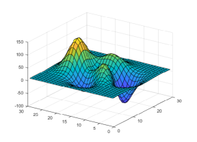
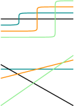
Figure 2: Left: Feasibility problem in 3d; are there $(x,y)\in\mathbb{R}^{2}$ such that $f(x,y)=0$? Middle: A pseudoline arrangement (top) and an isomorphic line arrangement (bottom). Right: A straight-line drawing of the complete $4$-partite graph $K_{2,2,2,2}$ with $8$ crossings, which is minimal for straight-line drawings. If the drawing does not have the be straight-line, six crossings are sufficient.

There is another way of defining $\exists\mathbb{R}$, which corresponds more closely to how (some) complexity classes have been defined traditionally, and that is through a machine model. For example,  was first defined as the class of problems solvable by non-deterministic polynomial time Turing machines, and then satisfiability was shown -complete. The -completeness of satisfiability, now known as the Cook-Levin theorem, laid the foundation of computational complexity. There is a Cook-Levin theorem for $\exists\mathbb{R}$ as well, if we define $\exists\mathbb{R}$ in the Blum-Shub-Smale (BSS) model of computation. Roughly speaking, in the BSS model of real computation we work with register machines that can read, store, and write real numbers in a single cell or register (with full precision), and perform exact arithmetic and comparisons on these numbers; registers can be pre-loaded with real constants. As inputs, BSS machines take tuples of real numbers (of arbitrary arity), so a BSS machine accepts a set of tuples of real numbers. In the BSS model, we can define polynomial time and non-deterministic polynomial time (real numbers have unit length and operations on real numbers take unit time). This allows a definition of problems that can be decided in polynomial time, $\P_{\mathbb{R}}$, and non-deterministic polynomial time, $\NP_{\mathbb{R}}$. If we restrict the non-deterministic machines so they are constant-free, that is, only constants $0$ and $1$ are allowed in the program code, and we only consider Boolean input tuples (all entries are $0$ or $1$) we obtain the complexity class $\BP(\NP_{\mathbb{R}}^{0})$. The original paper by Blum, Shub, and Smale [BSS89] already showed that the feasibility problem (with real coefficients) is complete for $\NP_{\mathbb{R}}$, this is the Cook-Levin theorem in the BSS model since it expresses a machine computation as a (real) satisfiability problem; the real Cook-Levin theorem easily implies that the feasibility problem we introduced earlier (with integer coefficients), is complete for $\BP(\NP_{\mathbb{R}}^{0})$, and this implies $\exists\mathbb{R}=\BP(\NP_{\mathbb{R}}^{0})$, so the BSS-model is a machine model for $\exists\mathbb{R}$.

As we will see in Section 3 on the history of the existential theory of the reals, these two alternative definitions arose independently.

We have defined ETR as a the existentially quantified subset of true sentences in the theory of the reals. In analogy with the polynomial-time hierarchy building on , we can similarly define a real polynomial hierarchy. The $Q_{1}\cdots Q_{k}$-fragment of the theory of the reals is defined by the true sentences which start with $k$ alternating blocks of quantifiers of the types $(Q_{1},\ldots,Q_{k})$, where $Q_{i}\in\{\exists,\forall\}$. The corresponding complexity classes are called $\Sigma_{k}\mathbb{R}$ and $\Pi_{k}\mathbb{R}$, depending on whether $Q_{1}=\exists$ or $Q_{1}=\forall$. The most common classes, apart from $\exists\mathbb{R}$, are $\forall\mathbb{R}=\Pi_{1}\mathbb{R}$, at the first level, and $\exists\forall\mathbb{R}=\Sigma_{2}\mathbb{R}$ and $\forall\exists\mathbb{R}=\Pi_{2}\mathbb{R}$ at the second level [SS23, JJ23]. These classes can also be defined in the BSS-model by considering alternating machines (machines with existential and universal states) or using an oracle model [M24].

Only a few problems have been shown complete for higher levels of the hierarchy (reflecting the situation for the polynomial-time hierarchy), we collect them in Section LABEL:sec:HigherLevels.

1.2 Where is the Existential Theory of the Reals?

We do not know much about the relationship of $\exists\mathbb{R}$ to traditional complexity classes, but we do know a little. Shor [S91] proved that $\NP\subseteq\exists\mathbb{R}$ by reducing satisfiability to stretchability; using ETR as the complete problem leads to an easier proof, since satisfiability can be expressed directly in ETR; for example, $(p\vee\overline{q}\vee r)\wedge(\overline{p}\vee\overline{r})$ can be expressed as $\exists p,q,r:(p=1\vee q=0\vee r=1)\wedge(p=0\vee r=0)$ in ETR.

The second result we know is due to Canny [C88, C88b], who in his thesis showed that $\exists\mathbb{R}\subseteq\PSPACE$ using his new notion of roadmaps.  is the class of problems decidable by (traditional) Turing machines in polynomial space. Complete problems for  include quantified Boolean formulas, and many game-related problems, such as Sokoban.

And this is all we know about $\exists\mathbb{R}$ with respect to traditional complexity classes. The status of $\exists\mathbb{R}$ with respect to , for instance, is wide open. The possibility that $\NP=\exists\mathbb{R}$ cannot yet be ruled out, but is usually considered unlikely. Natural polynomial-sized witnesses of positive instances of $\exists\mathbb{R}$-complete problems remain elusive. Furthermore, a number of possibly simpler problems which are not known to lie in  are contained in $\exists\mathbb{R}$. We review such problems now.

Inside $\exists\mathbb{R}$. $\exists\mathbb{R}$ contains several problems which are unlikely to be $\exists\mathbb{R}$-complete but are often relevant to $\exists\mathbb{R}$-complete problems. We discuss three of these problems here: the sum-of-square-roots problem, PosSLP and convex programming.

The sum-of-square-roots problem (SSQR) asks whether $\sum_{i\in[n]}a_{i}^{1/2}\geq k$ for positive integers $a_{1},\ldots,a_{n}$ and $k$. Clearly, $\textnormal{{SSQR}}\in\exists\mathbb{R}$, but this innocent-looking special case of $\exists\mathbb{R}$ has proved difficult to handle. There is a highly non-trivial upper bound on SSQR, via PosSLP which we discuss next, at the third level of the counting hierarchy (which is expected to be lower than , but way above ), see [ABKPM08]. This is a serious first obstacle in proving $\NP=\exists\mathbb{R}$, since we cannot even prove good upper bounds on SSQR, which belongs to the quantifier-free part of $\exists\mathbb{R}$. The SSQR-problem is powerful enough to solve some interesting problems in computational geometry: the complexity class $\P^{\textnormal{{SSQR}}}$ contains problems such as $3$-connected planar graph realizability for triangulations [CDR07, Theorem 1], as well as minimum-link path problems [KLPS17].

Also in $\exists\mathbb{R}$ and not known to lie in , is the Euclidean traveling salesperson problem (ETSP), in which we are given $n$ cities in the plane and ask for a shortest tour through all cities (in the Euclidean metric). It is often asked whether this problem is -complete; the obstacle to placing ETSP in  is the computation of the length of the route, which seems to require the solution of an SSQR-problem. The best upper bound on the Euclidean traveling salesperson is $\NP^{\textnormal{{SSQR}}}$. There are other problems that fall into this class, most prominently minimum weight triangulation, minimum dilation graphs, and the Steiner Tree problem [PS02, Section 10.4]; all of these problems are non-trivially -hard, see [P77, MR08, GGJ76, GKKKM10].

If the $n$ cities the Euclidean traveling salesperson must visit lie on an integer grid of size polynomial in $n$, then the problem lies in a slightly smaller class, $\NP^{\textnormal{{USSR}}}$, where USSR is the variant of SSQR in which the $a_{i}$ are given in unary (and this applies to grid versions of other problems in $\NP^{\textnormal{{SSQR}}}$ as well). Balaji and Datta [BD23] recently announced that $\textnormal{{USSR}}\in\Ppoly$, but this still does not imply that this grid version of the Euclidean salesperson lies in . It is quite possible that USSR and SSQR are polynomial-time solvable, and many researchers believe so, but their exact complexity remains open.

Let us turn to PosSLP, short for positive straight line program. A straight line program (SLP) is a finite sequence of instructions of the form $a_{0}=1$, and $a_{k}=a_{i}\oplus a_{j}$, where $i,j<k$ and $\oplus\in\{\cdot,+,-\}$. An SLP computes a sequence of numbers $(a_{k})_{k=0,\ldots,n}$. PosSLP asks whether $a_{n}>0$, that is, whether the final number computed by the SLP is positive. (For a related problem, see LABEL:p:UniFEAS). The value of $a_{n}$ may require exponentially many bits, since SLPs can perform repeated squaring, so PosSLP does not even obviously lie in , but it does, since PosSLP lies in $\exists\mathbb{R}$.

The best current upper bound on PosSLP is that, like SSQR, it lies in the third level of the counting hierarchy [ABKPM08]. One of the most striking results is that $\P^{\textnormal{{PosSLP}}}$, polynomial time on the word RAM with access to a PosSLP oracle, is as powerful as polynomial time on the real RAM on integer inputs [ABKPM08, Proposition 1.1]: the real RAM can run the SLP for PosSLP, since it can perform computations on reals, and therefore integers, in constant time; and we can simulate any real RAM algorithm on the word RAM using the PosSLP oracle whenever the program branches. This also implies that SSQR can be solved with oracle access to PosSLP, as the real RAM can solve SSQR.

In other words, PosSLP explains the gap between the word RAM and the real RAM. The currently best lower bound on PosSLP is by Bürgisser and Jindal [BJ24] and based on a bold conjecture. The second author conjectures that PosSLP also explains the gap between and $\exists\mathbb{R}$:

Conjecture.

$$\NP^{\textnormal{{PosSLP}}}=\exists\mathbb{R}.$$

PosSLP can be solved using semidefinite programming [ABKPM08], which is a special case of convex programming, and both of these belong to $\exists\mathbb{R}$. Thus the conjecture would also imply that convex programming is not polynomial time solvable unless $\NP=\exists\mathbb{R}$. Furthermore, since $\exists\mathbb{C}\subseteq\exists\mathbb{R}$ we get a better upper bound on the complexity of $\exists\mathbb{C}$. The current best bound, assuming the generalized Riemann hypothesis, is $\NP^{\RP}$ [Ko96]. Semidefinite programming also belongs to $\forall\mathbb{R}$ [SS23], so it lies in $\exists\mathbb{R}\cap\forall\mathbb{R}$, making it unlikely to be $\exists\mathbb{R}$-complete, unless $\forall\mathbb{R}=\exists\mathbb{R}$, which would be quite surprising. This also implies that $\exists\mathbb{R}$-complete problems, such as the rectilinear crossing number, cannot be solved using semidefinite programming, unless $\exists\mathbb{R}=\forall\mathbb{R}$. Junginger [JJ23] argues that polynomial identity testing also belongs to $\exists\mathbb{R}\cap\forall\mathbb{R}$ (it also lies in , randomized polynomial time).

		nondeterminism
		discrete	real
input	discrete		$\exists\mathbb{R}$
	real	$\textsf{DNP}_{\mathbb{R}}$	$\NP_{\mathbb{R}}$

Table 1: Complexity classes corresponding to discrete vs real inputs, and discrete (aka digital) vs real nondeterminism

Above $\exists\mathbb{R}$. If we look upwards from $\exists\mathbb{R}$, towards , we are at the start of a hierarchy, the real polynomial hierarchy. The finite levels of this hierarchy, such as $\exists\forall\mathbb{R}$ and $\forall\exists\mathbb{R}$, see LABEL:p:quantifiedR, still lie in  [BPR06, Remark 13.10], but the unbounded quantification of the full theory of the reals takes us outside of , to double exponential time (using Collins’ Cylindrical Algebraic Decomposition [C75]). In this survey we restrict ourselves to the finite levels of the hierarchy, but in the BSS-model there is structural research on the whole hierarchy, for example, an analogue of Toda’s theorem [BZ10]. One can also consider looking at mixing real and discrete quantifiers; in the BSS-model discrete quantifiers were studied under the name “digital nondeterminism”, leading to the class $\textsf{DNP}_{\mathbb{R}}$, the restriction of $\NP_{\mathbb{R}}$ to quantifiers over $\{0,1\}$, see the survey by Meer and Michaux [MM97] and Table 1. The Vapnik-Červonenkis dimension of a family of semialgebraic sets LABEL:p:semiVC is a natural problem that can be captured by mixed quantification [SS23, Section 4].

Another recent development is the introduction, by van der Zander, Bläser, and Liskiewicz [vdZBL23] of the complexity class succ$\exists\mathbb{R}$, a succinct version of $\exists\mathbb{R}$, which is allowed to encode arithmetic formulas using circuits. The class succ$\exists\mathbb{R}$ is the real analogue of , just like $\exists\mathbb{R}$ is the real analogue of  [BDLvdZ24]; it has turned out to be useful for studying problems in probabilistic reasoning, see [vdZBL23, DvdZBL24, BDLvdZ24, IIM24].

1.3 Universalities

$\exists\mathbb{R}$-completeness theory is closely related to an algebraic geometric notion usually referred to as universality. Informally, universality results state that spaces of solutions of simple geometric problems over the reals can behave “arbitrarily bad”. The occurrence of irrational numbers, and more generally numbers of arbitrary algebraic degree, or numbers requiring exponential precision, can sometimes be a hint towards universality, and $\exists\mathbb{R}$-hardness. In fact, algebraic universality can be seen as the strongest geometric statement about the intrinsic complexity of a realizability problem involving real numbers.

Irrationality.

The famous Perles configuration, described by Micha Perles in the 1960s, is composed of nine points and nine lines, with prescribed incidences, any realization of which in the Euclidean planes requires at least one irrational coordinate, see Figure 3.

Figure 3: The Perles configuration.

A much earlier example of such “nonrational” configurations with $11$ points was given by MacLane in 1936 [McL36], using von Staudt’s “algebra of throws”. Perles also constructed an $8$-dimensional combinatorial polytope that could be realized with vertex coordinates in $\mathbb{Q}[\sqrt{5}]$, but not with rational coordinates only [G03, Z08]. Much later, Brehm constructed three-dimensional polyhedral complexes, every realization of which requires irrational coordinates (see Ziegler [Z08]).

These three examples can be understood as early indications of the much more general universality property for point configurations, polytopes, and polyhedral complexes. In general, $\exists\mathbb{R}$-complete problems often require solutions of arbitrary high algebraic degree. Note, however, that this is not always the case; realizations of simple line arrangements, for instance, can always be slightly perturbed, but deciding the existence of one still remains $\exists\mathbb{R}$-hard. This leads us to the next topic.

Precision.

Pursuing the idea that solutions of simple geometric realizability problems may “behave badly”, let us note that ETR formulas of size $O(n)$ can encode doubly exponential numbers $x_{n}=2^{2^{n}}$ as follows

$$x_{0}=2,\ x_{i}=x_{i-1}^{2},\text{ for all }i=1,2,\ldots,n.$$

For $\exists\mathbb{R}$-complete geometric realizability problems, this implies that the number of bits, hence the precision, required to encode the coordinates of a realization, if one exists, can be exponentially large.

Early papers related to $\exists\mathbb{R}$-complete problems emphasized this precision issue. For instance Goodman, Pollack, and Sturmfels [GPS89, GPS90] showed two things: order types (combinatorial descriptions of point sets giving the orientation of every triple) can always be realized on an integer grid of double exponential size, and there are order types that need what they named “exponential storage”. The upper bound follows from the work of Grigorev and Vorobjov [GV89] (the “Ball Theorem”, see Section 2.1). Bienstock [B91] and later Kratochvíl and Matoušek [KM94] prove double exponential precision lower bounds for realizations with minimum crossing numbers and segment intersection graphs, respectively. Similarly, Richter-Gebert and Ziegler [RGZ95] explicitly state double-exponential lower bounds on coordinates for realizations of polytopes, and McDiarmid and Müller [McDM10, McDM13] actually cast this as the main result for unit disk graphs and disk graphs, while $\exists\mathbb{R}$-hardness is only mentioned in passing.

Like irrationality, the “exponential storage” phenomenon is a consequence of the much more general property of algebraic universality.

Algebraic Universality.

Algebraic universality is the culmination of those partial results on the “bad behavior” of polytopes and configurations of points and lines, and it is a property of the so-called solution, or realization spaces of a satisfiability problem over the reals.

In the stretchability problem, for instance, we are given the combinatorial type of an arrangement of $n$ pseudolines, consisting for example in the order, from left to right, of the intersection points of each pseudoline with the other $n-1$ pseudolines. The realization space is the set of all possible coordinates $(a_{1},b_{1},a_{2},b_{2},\ldots,a_{n},b_{n})\in\mathbb{R}^{2n}$ such that the $n$ lines of respective equations $y=a_{i}x+b_{i}$ realize the same arrangement. The famous universality result by Mnëv [M88] states that for every semialgebraic set $S$ there exists a pseudoline arrangement whose realization space is stably equivalent to $S$ [M88, RG99], where stable equivalence combines rational equivalence with so-called stable projections. Note that stable equivalence preserves the homotopy type and the algebraic number type, see [V23c, Section 4.1]. In particular, any topology can be preserved in that sense.

Maybe the simplest application of this theorem is to a semialgebraic set $S$ consisting of two points. Mnëv’s Theorem implies that there exists two arrangements of $n$ lines in the plane, where the orders of intersections are the same, but such that it is impossible to go continuously from one arrangement to the other without changing the combinatorial type in between. So Mnëv gives a strong negative answer to Ringel’s isotopy conjecture [R55, RG99].

This phenomenon of “disconnected realization spaces” had been observed before for polytopes [BG90]. Using Gale diagrams, Mnëv also gave a universality result for polytopes: Any semialgebraic set is stably equivalent to the realization space of a $d$-dimensional polytope with $d+4$ vertices. This gave rise to a series of results refining and generalizing Mnëv’s proof [RGZ95, RG96, RG99, PT14, APT15]. Richter-Gebert, in particular, dedicated a complete monograph on the universality of realization spaces of $4$-dimensional polytopes [RG96], implying that the problem of deciding whether a given lattice is realizable as the face lattice of a $4$-dimensional polytope is $\exists\mathbb{R}$-complete. The case $d=4$ is best possible: Steinitz Theorem gives a simple characterization of face lattices of three-dimensional polytopes that is decidable in polynomial time.

The exact definition of stable equivalence used in various contexts has varied over the years; recently it was pointed out that the definition used in Richter-Gebert’s text [RG96] required a fix [B22d, V23c].

While algebraic universality and $\exists\mathbb{R}$-hardness are closely related, they do not always imply each other: stable equivalences do not have to be effective (e.g. Datta [D03]), and $\exists\mathbb{R}$-hardness reductions rarely maintain stable equivalence. In many cases, stable equivalences can be made effective though; on the other hand, $\exists\mathbb{R}$-hardness results typically do not automatically yield algebraic universality results, but the proofs often allow the conclusion of weaker universality properties, e.g. Bienstock’s proof of $\exists\mathbb{R}$-hardness result for the rectilinear crossing number shows that every semialgebraic set occurs as the projection (not stable) of the realization space of a rectilinear crossing number problem. Our compendium indicates if universality results are known.

1.4 Proving $\exists\mathbb{R}$-Completeness

How can we tell whether a problem is a candidate for $\exists\mathbb{R}$-hardness? There are no hard-and-fast rules, but there are some tell-tale signs. First of all, there should be solutions to the problem that use real parameters. -hardness, without -membership can be a next clue: why does the problem not lie in , are real numbers the issue? To strengthen a suspicion of $\exists\mathbb{R}$-hardness, one can look for evidence of algebraic universality: can one construct instances that require algebraic solutions or rational solutions of exponential bitlength? None of these clues are sufficient, of course, for example, the Euclidean traveling salesperson problem is -hard and does not lie in , but it is unlikely to be $\exists\mathbb{R}$-hard, since it belongs to $\NP^{\textnormal{{SSQR}}}$; and representing a plane graph as a disk contact graph may require algebraic radii, but testing planarity can be decided in linear time. Topological universality can also be misleading, there are problems in that exhibit topological universality [SW23, BEMMSW22, ST22].

$\exists\mathbb{R}$-Membership

Since ETR is a very expressive language, it is typically not difficult, though sometimes cumbersome, to establish membership in $\exists\mathbb{R}$, and we can even use the result of ten Cate, Kolaitis, and Othman [tCKO13, Theorem 4.11] that ETR is closed under -many-one reductions, for example, see  LABEL:p:totvardistMDP and LABEL:p:satprobL.

Compare this situation to . We can show membership by encoding the problem as a satisfiability problem, yet it is often easier to show that the problem can be accepted by a Turing machine in non-deterministic polynomial-time. Or we can even work in the word RAM model, which allows random access to an unlimited number of registers storing integers on which we can perform arithmetical operations.

Erickson, van der Hoog, and Miltzow [EvdHM20]) showed that we have the same option for $\exists\mathbb{R}$: if we replace the word RAM by a real RAM, which allows us to guess real, not just discrete, numbers and has unlimited storage for real numbers, we obtain $\exists\mathbb{R}$. The real RAM model can simplify $\exists\mathbb{R}$-membership arguments significantly, as describing an algorithm is much easier than writing down an ETR formula, and researchers can make use of the huge number of real RAM algorithms already developed in computational geometry and other areas.

Efficient membership proofs may also lead to algorithmic solutions of problems, e.g. Dean [D02] showed how to express the rectilinear crossing number problem as an optimization problem with linear constraints. While solvers for these problems may not yet be as fast as solvers for , where a linear programming formulation for the (topological) crossing number problem has been implemented and can compute crossing numbers of reasonably large graphs on the web [CW16], this may very well change in the future.

$\exists\mathbb{R}$-Hardness

In this section, we discuss two primary techniques to show $\exists\mathbb{R}$-hardness, one based on algebra, and the other on geometry. The first technique, we refer to as algebraic encoding, involves encoding real variables, addition and multiplication directly. The second technique, known as stretchability encoding, is based on encoding the stretchability problem.

Algebraic Encoding.

Algebraic encoding work by encoding algebraic constraints on variables, such as $x=y+z$ and $x=yz$; so in a first step, we need to encode real variables. How to do so is problem-specific but often straightforward. For instance, in the art gallery problem we can encode variables by using the coordinates of a guard’s position, see Figure 4 for an illustration.

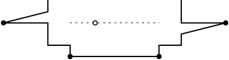
Figure 4: The white guard needs to be placed anywhere on the dotted line segment in order to see all the marked vertices. We can interpret the position of the guard as a value in a real-valued interval.

Similarly, to show stretchability $\exists\mathbb{R}$-hard, we can work with the parameters of the lines, or the coordinates of the intersections.

It is often useful to know that the variables we need to encode can be assumed to be bounded, e.g. ETR-INV LABEL:p:ETRINV allows us to assume that all variables belong to the interval $[1/2,2]$. Bounded variables can be encoded in the coordinates of a geometric object with limited range, such as a guard in an art gallery. One can even reduce the range to much smaller intervals, such as $[0,n^{-200}]$, where $n$ is the size of the input. This may seem counter-intuitive as it leaves very little wiggle room for the variables, but because we can encode variables with very high precision, it is sufficient.

Secondly, we encode addition, of the form $x=y+z$. This is typically simple as it is a linear relation between three variables. For geometric problems, addition can often be encoded by forcing two geometric objects to lie next to each other, e.g. two pieces in the packing problem, with the combined object encoding the sum.

Remark (Addition with von Staudt).

Many proofs work with variants of the von Staudt gadgets originally used by Mnëv [M88] to show that order type LABEL:p:ordertype, and thereby stretchability LABEL:p:Stretch, is universal. Figure 5 shows a simplified von Staudt addition gadget on the left. Variables are encoded as length of segments (starting at $0$). Assuming the drawing of the gadget satisfies that $0,y,z$ and $x$ are collinear and $pq\parallel 0x$, $0p\parallel zq$ and $py\parallel qx$, then $x=y+z$.

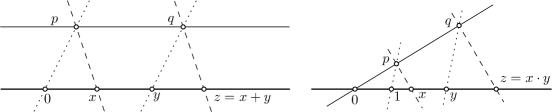
Figure 5: Simplified von Staudt addition gadget, left, and multiplication gadget, right. The original gadgets are projective, not Euclidean.

In some rare cases, though, the encoding of addition is trickier, as, for example, in the case of the boundary-guarding variant of the art gallery problem; addition here is the main obstacle as there is no direct interaction of three guards at all, so it is not obvious how to encode a ternary relation.

Thirdly, we need to encode multiplication, i.e., $x=y\cdot z$.

Remark (Multiplication with von Staudt).

Figure 5 shows how multiplication can be encoded using von Staudt gadgets (again simplified, removing the projective setting): as long as $0pq$ and $01zyx$ are each collinear, but distinct, and $p1\parallel qz$ and $py\parallel qx$, we have $x=y\cdot z$. It follows that geometric problems that can express parallelism and collinearity are $\exists\mathbb{R}$-hard. By interpreting the von Staudt gadgets in the projective plane (as von Staudt and Mnëv’s did), both collinearity and parallelism can be expressed using order types.

Encoding multiplication directly can be tricky, but it can be simplified by simulating multiplication through inversion, as is done in ETR-INV LABEL:p:ETRINV. To see how to do this, note that

$$(y+z)^{2}-(y-z)^{2}=4x$$

is equivalent to

$$x=y\cdot z.$$

Which indicates that multiplication can be simulated by squaring, i.e., $x=y^{2}$. Consider

$$\frac{1}{\frac{1}{x-1}-\frac{1}{x}}+x=x^{2}.$$

This identity shows that inversion, i.e. $x\cdot y=1$ , is sufficient to encode squaring. Inversion is often much easier to encode compared to multiplication as it involves only two variables in a symmetric way.

The inversion constraint can be replaced by almost any non-linear constraint [MS24] of the form

$$f(x,y)=0,$$

see LABEL:p:CSSP. Although, this is very powerful, we are only aware of one application, namely showing that geometric packing LABEL:p:geopack, packing convex polygons into a square container, is $\exists\mathbb{R}$-complete [AMS20]. The idea of the proof is that any non-linear constraint that is sufficiently smooth can be very well approximated by the first two terms of the Taylor series in a sufficiently small neighborhood. And the first two terms of the Taylor series are just a quadratic equation.

Finally, we need to connect the variables to the different gadgets. This step, which looks like simple housekeeping, can be surprisingly challenging in many reductions. As Richter-Gebert writes in [RG96]:

The main difficulty in Mnëv’s proof is to organize the construction in a way such that different basic calculations do not interfere and such that the underlying oriented matroid stays invariant for all instances of a geometric computation.

To see what the issue is, recall the von Staudt gadget for addition (or multiplication) in Figure 5. If we want to encode the gadget using order types, we need to know whether $x<y$, $x=y$ or $x>y$. How would we know? And even if we did, how would we know for other, intermediate variables? This problem has been solved using various normal forms; maybe the most elegant solution is due to Richter-Gebert [RG96], this is the approach presented by Matoušek [M14].

It can also be helpful to know that the variable-clause incident graphs are of a restricted type, for example planar, as in PLANAR-ETR-INV LABEL:p:PlanarETRINV.

Stretchability Encoding.

The stretchability problem LABEL:p:Stretch asks whether a given pseudoline arrangement can be stretched, that is, if there is an equivalent line arrangement, that is a line arrangement which has the same combinatorial structure.

Figure 6: A (stretchable) pseudoline arrangement on the left, and an equivalent line arrangement on the right.

Reductions from stretchability are particularly popular in the graph drawing and computational geometry community. The segment intersection graph problem LABEL:p:SEG is an early example: we can represent each pseudoline by a segment and surround each pseudoline-segment with additional segments which enforce the combinatorial structure of the pseudoline arrangement, see Figure 7.

Figure 7: Forcing the combinatorial structure of a pseudoline arrangement using segment intersections.

If there is a representation of the graph using segments then the underlying pseudoline arrangement is stretchable, see [KM94, S10]. Another, earlier, example due to Bienstock [B91] shows how to embed stretchable arrangements in the rectilinear crossing number problem.

1.5 What is next for $\exists\mathbb{R}$?

In this section, we want to point at possible future research directions that appear of interest to us. We focus on broad research lines, for specific candidate problems see LABEL:sec:Candidates.

Breadth.

Most of the early $\exists\mathbb{R}$-complete problems arose in graph drawing and algebraic complexity. As the compendium shows, many more areas like probabilistic reasoning, machine learning, polytope theory etc. have been added since then, and it seems reasonable to believe that this trend continues and that more $\exists\mathbb{R}$-complete problems are found in other research areas.

Depth.

After a problem has been shown $\exists\mathbb{R}$-complete, we can start asking whether more restricted versions of the problem remain $\exists\mathbb{R}$-complete. This is particularly important for problems that are common starting points for reductions; for , this is evidenced by the numerous satisfiability variants that have been shown -complete. For $\exists\mathbb{R}$, the original ETR LABEL:p:ETR has been refined in many ways, including the many variants of ETR-INV LABEL:p:ETRINV which have significantly simplified reductions for many problems.

Similarly, the partial version of order type realizability LABEL:p:ordertype was introduced in [S21b] to show that many problems remain hard if some parameters are constant. To give an example, the simultaneous geometric embedding LABEL:p:SGE is $\exists\mathbb{R}$-complete [CK15], and it is now known that it remains so, even if the number of input graphs is bounded, indeed at most $31$ [FKMPTV24, S21b], or all the input graphs are edge-disjoint [KR23]. There are many examples like this already, and we expect that many more problems with constant natural parameters will be shown $\exists\mathbb{R}$-complete.

Parameterized Theory of $\exists\mathbb{R}$.

Many -complete problems become considerably easier, if some of their parameters are bounded, the point of view taken by the area of parameterized complexity.

For example, we can decide whether a graph on $n$ vertices contains a vertex cover of size at most $k$ in time $O(2^{k}n^{2})$. For fixed $k$, this gives a quadratic-time algorithm for the vertex cover problem. Even if $k$ is not fixed, but small compared to $n$, this running-time is a tremendous speed-up to the general worst-case complexity of $O(c^{n})$. We are not aware of a single $\exists\mathbb{R}$-complete problem with a running time of $f(k)n^{O(1)}$ for some natural parameter $k$. It would be interesting to see if such a problem exists and what type of parameterization is required. On the other hand, we are aware of some $\exists\mathbb{R}$-complete problems for which the parameterized version is $W[1]$-hard [ArtParaHard]. It would be interesting to be able to find the correct parameterized complexity class for those problems.

Structural Complexity.

The study of structural properties of complexity classes has matured since  was first introduced, see for instance the book by Arora and Barak [arora2009computational]. Structural questions have been studied widely in the BSS-model of computation, starting with the book by Blum, Cucker, Shub and Smale [BCSS98]; for a more recent survey, see Baartse and Meer [BM13]. Yet, for many classical results, we do not have analogue results for $\exists\mathbb{R}$ or the real hierarchy. To list some examples:

• Does $\forall\mathbb{R}=\exists\mathbb{R}$ imply that the real hierarchy collapses? This would follow from showing that $\forall\mathbb{R}\cap\exists\mathbb{R}$ is low for $\exists\mathbb{R}$, that is $\exists\mathbb{R}^{\forall\mathbb{R}\cap\exists\mathbb{R}}=\exists\mathbb{R}$; to make these statements meaningful, we need to work with a model for $\exists\mathbb{R}$ that allows for oracles, see [M24].

• Fagin’s theorem characterizes  as the set of properties captured by monadic second-order logic. Can we characterize $\exists\mathbb{R}$ in a similar fashion? There is a similar theorem for $\NP_{\mathbb{R}}$, see [MM97, Section 7].

• Toda’s theorem, that the polynomial-time hierarchy reduces to , probabilistic polynomial time, was a breakthrough result in classical complexity theory [arora2009computational, Theorem 17.4]. Basu and Zell [BZ10] showed that the result can be adopted to the BSS-model. Is there a discrete analogue for the real hierarchy?

• Are there oracles relative to which $\NP=\exists\mathbb{R}\neq\PSPACE$ or $\NP\subsetneq\exists\mathbb{R}$?

• What are the connections between $\exists\mathbb{R}$ and other complexity classes defined to capture working with continuous solution spaces? Specifically, how does $\exists\mathbb{R}$ relate to CLS [CLS-intro] and FIXP [EY10]? This can be studied by looking at finding a Nash Equilibrium problem which is either $\exists\mathbb{R}$-complete or FIXP-complete, depending on the technical details of the definition.

We expect positive answers to many of these questions, and some of them may not be that difficult.

Counting Complexity.

A counting version of $\exists\mathbb{R}$ was introduced by Bürgisser and Cucker [BC06] as $\BP(\#\P_{\mathbb{R}}^{0})$, which we could call $\#\mathbb{R}$; they show that counting the number of points in a semialgebraic set is complete for this class, and computing the Euler-Yao characteristic of a semialgebraic set is complete for this class under Turing reductions. The paper leaves many interesting open questions, not least of it being the question of where $\#\mathbb{R}$ is located with respect to traditional complexity classes.

Better Techniques to Show Hardness.

Reductions for $\exists\mathbb{R}$-hardness tend to start with a relatively small set of problems. Maybe the three most prominent starting problems are simple stretchability LABEL:p:Stretch, feasibility LABEL:p:feasibility and ETR-INV LABEL:p:ETRINV.

Simple stretchability is useful as a very geometric problem that has turned out to be very adaptable to different contexts; one advantage it has (particularly over stretchability) is that its solution space is open, which is the case for many geometric problems. ETR-INV is quite versatile and can be adapted to many situations: the range of variables can be bounded, multiplication can be replaced by inversion. Feasibility has served as the starting point for nearly all problems from algebraic geometry and analysis; that may not be that surprising, since it is the oldest and best-studied problem.

These results can be refined even further. Instead of Stretchability, we can now use pseudo-segment stretchability LABEL:p:SegStretch. This makes the reduction more tedious, but it allows to bound certain parameters by a constant [S21]. Similarly, the inversion in ETR-INV can be replaced by virtually any curved function [MS24]. In analogy with , we expect that the core problems will be further refined to become more flexible, easier to apply, and yield stronger results.

Real Hierarchy.

There is a small number of papers that study the real polynomial time hierarchy starting with a paper by Bürgisser and Cucker [BC09] in the BSS-tradition. Some fundamental problems like the Hausdorff distance are complete for the second level of this hierarchy [JKM22]. Studying the second level of the hierarchy is more challenging as many standard techniques that can be used for the first-level are not yet known to work for the second-level.

Developing techniques for higher levels of the hierarchy and identifying additional natural problems captured by these levels appear of interest to us. There are also structural questions, for example related to the power of exotic quantifiers that have not been answered yet.

Unifying Algorithmic Techniques.

Although, $\exists\mathbb{R}$ is a relatively new complexity class, the problems that are complete for it have a very long and rich history. Yet, the study of different algorithms for $\exists\mathbb{R}$-complete problems is almost independent. For instance, neural networks with billions of parameters are routinely trained in industry applications; the insights and techniques developed in this application of gradient descent to neural networks seem to have little effect on the way that the graph drawing community is drawing graphs. See [Stress-Minimization, GD-squared] for some first work to transfer knowledge from machine learning to graph drawing. For -complete problems algorithmic techniques that work well for one problem also work well for another problem. Therefore, those problems are often studied together. Yet the graph drawing, packing, and machine learning community are almost disjoint.

It may be the case that the problem-specific differences are more important for $\exists\mathbb{R}$-complete problems and thus a more unified approach might just not be very fruitful. Even then it would be nice to capture this in some way.

2 A Toolbox for $\exists\mathbb{R}$

In this section we review some tools that have shown themselves useful in various aspects of $\exists\mathbb{R}$-completeness, including the ball and gap theorems, which allow us to juggle with equalities and inequalities, quantifier elimination, and exotic quantifiers, which extend the language of the theory.

2.1 The “Ball Theorem”

The original “ball theorem” is due to Vorobev and Grigoriev [V84, GV89]. The following statement is weaker than the currently best known results, see [BR10, Theorem 3], but sufficient for all of our applications to the existential theory of the reals. A version stated for semialgebraic sets can be found in [SS17, Corollary 3.4], and Renegar [R92, Proposition 1.3] stated a version which is useful at higher levels of the hierarchy.

Theorem 2.1 (Vorobev and Grigoriev).

If $f_{i}\in\mathbb{Z}[x_{1},\ldots,x_{n}]$, $i\in[k]$ is a family of polynomials with coefficients of bitlength at most $L$ and total degree at most $d$, then every connected component of $\{x\in\mathbb{R}^{n}:f_{i}(x)\geq 0$ for all $i\in[k]\}$ intersects the ball of radius $2^{(L+\log{k})d^{cn}}$, for some constant $c>0$ independent of $f$.

We want to point out that this theorem relies on the coefficients being integers. If they are real numbers then no upper bound on the radius is known. To see the difficulty to translate such a result to real coefficients consider the linear equation $aX-bX=1$. The solution is $X=\tfrac{1}{a-b}$, which can be arbitrarily large.

The innocent-looking Theorem 2.1 has some far-reaching consequences. To start with, it can be used to write a decision algorithm for $\exists\mathbb{R}$ that runs in exponential time [GV89].

The ball theorem also implies that solutions to computational problems in $\exists\mathbb{R}$ can be bounded in size. As an example, consider the order type realizability problem LABEL:p:ordertype. One way to measure the size of a solution of a geometric problem like order type realizability is by working with area; to make this notion non-trivial—a realizable order type can be realized in any arbitrary small region—one typically adds some resolution requirement, say that the points must have at least unit distance. We can then define the area of a realization to be the area of a smallest bounding box; the area of a realizable instance of order type then is the smallest area of a realization in which every pair of points has distance at least one. The following result, stated for spread rather than area, can be found in Goodman, Pollack, and Sturmfels [GPS90, Theorem 2].

Theorem 2.2 (Goodman,Pollack, and Sturmfels).

A realizable order type on $n$ points can be realized in area $2^{2^{O(n)}}$, and there are order types that require area $2^{2^{\Omega(n)}}$.

The proof is conceptually simple: we can express the realizability of an order type on points $(p_{i})_{i\in[n]}$ as the feasibility of a system of quadratic polynomials $f_{i}(p)\geq 0$, $i\in[k]$, where $k=O(n)$. We add $O(n^{2})$ polynomial conditions of the form $\lVert p_{i}-p_{j}\rVert^{2}-1\geq 0$ to enforce the minimum resolution. By Theorem 2.1, there is a solution in which all variables have distance at most $R=2^{2^{O(n)}}$ from the origin; in particular, this applies to the coordinates of the points $(p_{i})_{i\in[n]}$, implying the area upper bound.

The main obstacle to upper bounds like this is, occasionally, the encoding of the conditions in ETR. A recent example is right-angle drawability [B20, S23b]. This issue becomes even more intricate if one aims at optimal bounds. This can require significant additional work, see, for example, the papers by McDiarmid and Müller [McDM13] and Kang and Müller [KM12].

Goodman, Pollack, and Sturmfels [GPS90] also proved the corresponding lower bound, using a construction that lends itself to adaptation to other settings. Double-exponential lower bounds were reproduced in several early papers for various problems including rectilinear crossing number LABEL:p:rectcross in [B91], segment intersection graphs LABEL:p:SEG in [KM94], and realizability of $4$-polytopes LABEL:p:4DPolytope in [RGZ95]. For most $\exists\mathbb{R}$-hardness reductions, double-exponential precision carries over, so these lower-bound results are nearly automatic, and are rarely stated explicitly these days, unless extra work is required.

Because the order type problem is universal, we cannot expect its realizations to be possible on a grid, but if we restrict ourselves to point sets in general position, so no three points are collinear, then there always is a solution on a grid.

Theorem 2.3 (Goodman,Pollack, and Sturmfels).

If an order type is realizable by $n$ points in general position, then there is a realization on a grid of size $2^{2^{O(n)}}\times 2^{2^{O(n)}}$, and there are order types that require grids of size $2^{2^{\Omega(n)}}\times 2^{2^{\Omega(n)}}$.

The proof extends the proof of Theorem 2.2 with a careful analysis on how far points can be perturbed without changing the order type. Kachiyan and Porkolab [KP97, Corollary 2.6] observed that work by Basu, Pollack and Roy implies the general result that every open (actually, every full-dimensional) semialgebraic set always contains a rational point of at most exponential complexity. This automatically applies to any problem in $\exists\mathbb{R}$ whose solution space is open, such as the simple stretchability LABEL:p:Stretch and the rectilinear crossing number LABEL:p:rectcross. In the case of right-angle drawings with one bend, a similar upper bound can be obtained even though the realization space is not open [S23b, Theorem 15].

Tarski showed that his quantifier elimination algorithm works over an arbitrary real-closed field, implying that a formula can be satisfied over $\mathbb{R}$ if and only of it can be satisfied over the algebraic numbers (which are real-closed). It follows that any non-empty semialgebraic set contains an algebraic point. Kachiyan and Porkolab [KP97, Proposition 2.2] strengthened this result by showing that (non-empty) semialgebraic sets always contain algebraic points of at most exponential complexity; that is, there is an exponential bound on the size of a (Thom) encoding of such a point. This conclusion applies to most of the remaining problems, such as stretchability LABEL:p:Stretch and the art gallery problem LABEL:p:ArtGallery.

Theorem 2.1 can also be used to show that feasibility LABEL:p:feasibility remains $\exists\mathbb{R}$-complete if restricted to a compact domain, say $[-1,1]^{n}$. As far as we know, this was first shown by Schaefer [S13, Lemma 3.9], and there is no result like this (for compact domains) for $\NP_{\mathbb{R}}$.

Theorem 2.4 (Schaefer).

Testing whether a polynomial $f\in\mathbb{Z}[x_{1},\ldots,x_{n}]$ has a root in $[-1,1]^{n}$ is $\exists\mathbb{R}$-complete.

For open domains, like $(-1,1)^{n}$, the proof is much simpler, since $z\mapsto\frac{z}{1-z^{2}}$ is a surjective map from $(-1,1)$ to $\mathbb{R}$, but there cannot be a continuous surjective map from $[-1,1]$ to $\mathbb{R}$, since the image of such a map would be compact. An extension of this result to the second level of the hierarchy was obtained by D’Costa, Lefaucheux, Neumann, Ouaknine, and Worrellin [DCLNOW21, Lemma 10] and Jungeblut, Kleist, and Miltzow [JKM22].

We will look at further consequences of Theorem 2.1 in Section 2.2, where we will see how it can be combined with gap theorems to replace equalities with strict inequalities. It can also be used to remove the exotic H-quantifier, see Lemma 2.9.

2.2 Gap Theorems

Gap theorems establish lower bounds on the distance between two algebraic objects that have positive distance. One of the oldest is Cauchy’s theorem which establishes upper and lower bounds on roots of a univariate polynomial [Y00]. This can be generalized, under certain assumptions, to multivariate polynomials, as was done for example by Canny [C88, C88b]. One can derive the multivariate separations via quantifier elimination from Cauchy’s theorem, but there are also direct proofs. The following theorem follows from a strong separation result due to Jeronimo and Perruci [JP09], the simple derivation can be found in [SS17, Corollary 3.6].

Theorem 2.5 (Jeronimo, Perruci).

If $f\in\mathbb{Z}[x_{1},\ldots,x_{n}]$ is a polynomial with coefficients of bitlength at most $L$ and total degree at most $d$, for which $\inf_{x\in\mathbb{R}^{n}}f(x)>0$, then

$$\inf_{x\in\mathbb{R}^{n}}f(x)>2^{-(Ln^{d}+1)d^{n+1}}d^{-(n+1)d^{n+1}}.$$

With this theorem, one can establish useful separation bounds for semialgebraic sets, e.g. the following bound from [SS17, Corollary 3.8]. For a formula $\varphi$ we write $|\varphi|$ for its bitlength.

Lemma 2.6 (Schaefer, Štefankovič).

Suppose the distance between two semialgebraic sets $S=\{x\in\mathbb{R}^{n}:\varphi(x)\}$ and $T=\{x\in\mathbb{R}^{n}:\psi(x)\}$ is positive. Then that distance is at least $2^{-2^{L+5}}$, assuming $L:=|\varphi|+|\psi|\geq 5n$.

Combining this separation with Theorem 2.1 one can show that testing whether $f(x)>0$ for all $x\in\mathbb{R}^{n}$ for a given polynomial $f$ is $\forall\mathbb{R}$-complete LABEL:p:GlobalPos: Given $f$, if $f(x)=0$ for some $x\in\mathbb{R}^{n}$, then by Theorem 2.1, there is an $x\in[-R,R]^{n}$, where $R=2^{2^{O(L)}}$ and $L$ is the bitlength of $f$. Consider the sets $S=\{(x,y)\in\mathbb{R}^{n+1}:f(x)=y,x\in[-R,R]^{n}\}$ and $T=\{(x,0):x\in[-R,R]^{n}\}$. If $f(x)=0$ for some $x$, then the distance of $S$ and $T$ is $0$, otherwise, the distance is positive (since both sets are compact), and so by Lemma 2.6 that distance is at least $2^{-2^{O(L)}}$. Here we use repeated squaring to express $R$ in the definition of $S$ and $T$, and we can also use it to express a lower bound $\delta>0$ on the distance of $S$ and $T$ (if $f(x)>0$) of bitlength at most $O(L)$. It follows that $f(x)=0$ for some $x\in\mathbb{R}^{n}$ if and only if $|f(x)|<\delta$ for some $x\in\mathbb{R}^{n}$. It follows that strict global positivity LABEL:p:GlobalPos is $\forall\mathbb{R}$-complete.

Since this idea allows us to replace equalities with strict inequalities, it also follows that ETR remains $\exists\mathbb{R}$-complete even if equality and negation are not allowed. This result, proved in [SS17], is an indication that the definition of $\exists\mathbb{R}$ is quite robust. It implies, as we mentioned earlier, that problems which can be defined without equality, like simple stretchability and segment intersection graphs have the same computational complexity as problems like feasibility and stretchability, which use equality.

A similar approach was used by Bürgisser and Cucker [BC09] to eliminate the exotic H-quantifier, see Lemma 2.9 below.

We saw that $f(x)=0$ can be equivalently replaced by $f(x)<\varepsilon$, where $\varepsilon$ is a doubly exponential small constant (depending on $f$). Another way of reading this is that finding an approximate solution to the feasibility problem, with a double exponential error, is as hard as the feasibility problem itself. This type of statement could be made for nearly every $\exists\mathbb{R}$-complete problem, though it is rarely made explicitly. Examples include drawings which are nearly right-angle drawings LABEL:p:racdraw, and approximating the Hausdorff distance LABEL:p:Hausdorffdist to within a double-exponential error.

2.3 Quantifier Elimination

Suppose we are given a two-dimensional region $S=\{x\in\mathbb{R}^{2}:\varphi(x)\}$ and we want to determine whether $S$ has diameter at most $1$. How hard is that? Using the first-order theory of the reals, we can express the diameter condition as

$$(\forall x,y\in\mathbb{R}^{2})\ x\in S\wedge y\in S\rightarrow\lVert x-y\rVert\leq 1.$$

Let us be a bit more honest and replace $\in S$ with $\varphi$, and eliminate the hidden square roots in $\lVert\cdot\rVert$. That gives us

$$(\forall x,y\in\mathbb{R}^{2})\ \varphi(x)\wedge\varphi(y)\rightarrow\lVert x-y\rVert^{2}\leq 1.$$ (1)

We can decide the truth of that sentence by using quantifier elimination. There are very sophisticated quantitative versions of quantifier elimination depending on the number of variables, degree of polynomials, and other parameters. For our purposes, a very simple version, which only eliminates a single quantifier is sufficient. This version follows, for example, from [BPR06, Algorithm 14.5], and that reference presents many more variants. As earlier, we write $|\Phi|$ for the bitlength of formula $\Phi$.

Lemma 2.7.

Let $\Phi(x,y)$ be a quantifier-free formula, with $x\in\mathbb{R}$ and $y\in\mathbb{R}^{n}$. In time $|\Phi|^{O(n)}$ one can construct a formula $\Psi(y)$, of size $|\Phi|^{O(n)}$, such that

$$(\exists x\in\mathbb{R})\ \Phi(x,y)\ \leftrightarrow\Psi(y).$$

The lemma allows us to remove one quantifier at a time, and it can be used for both existential and universal quantifiers (using negation). Applying the lemma four times (twice for each point) to (1) yields, in polynomial time since $n$ is bounded, a variable-free formula whose truth can then be evaluated in polynomial time. So having diameter at most $1$ can be decided in polynomial time for semialgebraic sets in $\mathbb{R}^{2}$, since there is only a constant number of quantifiers that need to be eliminated. An analogous argument works for every fixed dimension $d$. If $d$ is part of the input, so not fixed, then the problem becomes $\forall\mathbb{R}$-complete LABEL:p:diamsemi. Eliminating quantifiers no longer works in polynomial time in this case, since we have $\Theta(d)$ many variables. Quantifier elimination still gives us an (exponential-time) decision procedure, of course.

Quantifier elimination can be used to show that a large number of problems are polynomial-time solvable in fixed dimension; this includes problems like convexity LABEL:p:convexity, radius LABEL:p:radiussemi, Brouwer fixed point LABEL:p:BrouwerFixedPoint, and many variants of the Nash equilibrium problem, see Section LABEL:sec:Nash.

2.4 Replacing Exotic Quantifiers

Sometimes problems are not captured well by traditional quantifiers. Let us have a closer look at the dimensionality problem of semialgebraic sets. A semialgebraic set $S\subseteq\mathbb{R}^{d}$ is full-dimensional if it contains an open subset, or, equivalently, an open ball. We can express this formally as

$$(\exists x\in\mathbb{R}^{d})(\exists\delta\in R)(\forall y\in\mathbb{R}^{d})\ \lVert y-x\rVert<\delta\rightarrow y\in S.$$

So testing whether $S$ is full-dimensional lies in $\exists\forall\mathbb{R}$, the second level of the hierarchy. The condition can be expressed more succinctly using $\exists^{*}$, one of the exotic quantifiers introduced by Koiran [K99], $(\exists^{*}x\in\mathbb{R}^{d})\ \varphi(x)$ is defined as $(\exists x\in\mathbb{R}^{d})(\exists\delta\in\mathbb{R}_{>0})(\forall y\in\mathbb{R}^{d})\ \lVert y-x\rVert<\delta\rightarrow\varphi(y)$. With that, our characterization of full-dimensionality of $S$ simplifies to

$$(\exists^{*}x\in\mathbb{R}^{d})\ x\in S.$$

Koiran then went on to show that $\exists^{*}$ can be replaced with $\exists$ by adding some variables, also see [BC09, Section 8]:

Lemma 2.8 (Koiran).

Given a formula $\Phi(x,y)$ in prenex form with a fixed number of quantifier alternations, one can in polynomial time construct a formula $\Psi(x^{\prime},y)$ such that

$$(\exists^{*}x\in\mathbb{R}^{d})\ \Phi(x,y)\ \leftrightarrow(\exists x^{\prime}\in\mathbb{R}^{d^{\prime}})\ \Psi(x^{\prime},y),$$

$d^{\prime}$ is polynomially bounded in $d$, and $\Psi(x^{\prime},y)$ has the same pattern of quantifier alternations as $\Phi(x,y)$.

For the full-dimensionality example we can let $\Phi$ be the defining formula of $S=\{x\in\mathbb{R}^{d}:\varphi(x)\}$, so there are no additional quantifiers or variables. It follows that being full-dimensional lies in $\exists\mathbb{R}$, and it is easily seen to be $\exists\mathbb{R}$-hard, so the real dimension of a semialgebraic set LABEL:p:dimension is $\exists\mathbb{R}$-complete.

The second exotic quantifier, $\forall^{*}$, is the negation of $\exists^{*}$, so it intuitively corresponds to saying “for a dense set”, and, as the negation of $\exists^{*}$ can be replaced by $\forall$ using Koiran’s lemma.

Koiran’s result significantly extends the expressive power of the existential theory of the reals and has been used for other examples including positivity LABEL:p:GlobalPos, continuity LABEL:p:ContinuityAC, and image density LABEL:p:imagedensity, also see [BC09, Table 2].

The third exotic quantifier, H, is a bit different. Whereas $\exists^{*}$ and $\forall^{*}$ are concerned with density, H is concerned with limits, and tends to appear when suprema or infima are involved.

Define $(\textup{{H}}\varepsilon)$ as $(\exists\varepsilon^{\prime}>0)(\forall\varepsilon\in(0,\varepsilon^{\prime}))$; H can be read as “for all sufficiently small $\varepsilon$”; it is introduced in Bürgisser and Cucker [BC09]. We saw earlier that having diameter at most $1$ lies in $\forall\mathbb{R}$. What about requiring the diameter to be strictly less than $1$? It is not sufficient to say

$$(\forall x,y\in\mathbb{R}^{d})\ x\in S\wedge y\in S\rightarrow\lVert x-y\rVert<1,$$

since the diameter is the supremum of the distances of points in $S$. The H-quantifier offers a solution:

$$(\textup{{H}}\varepsilon>0)(\forall x,y\in\mathbb{R}^{d})\ x\in S\wedge y\in S\rightarrow\lVert x-y\rVert\leq 1-\varepsilon,$$

By a result of Bürgisser and Cucker [BC09, Theorem 9.2], a leading H-quantifier can be eliminated.

Lemma 2.9 (Bürgisser, Cucker).

Let $\Phi(\varepsilon)$ be a formula in prenex form. We can construct a formula $\Psi$ in polynomial time such that

$$(\textup{{H}}\varepsilon>0)\ \Phi(\varepsilon)$$

is equivalent to $\Psi$, and $\Psi$ has the same pattern of quantifier alternations as $\Phi(\varepsilon)$.

In particular, if $\Phi$ is an existentially or universally quantified formula, then so is $\Psi$. (This special case was independently discovered by Schaefer, Štefankovič [SS17], already used in [S13].) From this we can conclude that the diameter problem lies in $\forall\mathbb{R}$.

Other computational problems that have been placed in $\exists\mathbb{R}$ or $\forall\mathbb{R}$ using the elimination of a leading H-quantifier, including several properties of semialgebraic sets such as unboundedess LABEL:p:unbounded, a specific point belonging to the closure of a set LABEL:p:ZeroinClosure, linkage rigidity LABEL:p:linkagerigid, a point not being an isolated zero of a polynomial LABEL:p:ISO, and the distance of semialgebraic sets LABEL:p:distancesemi. An example from a different area is the angular resolution of a graph LABEL:p:angularres, which is defined with a supremum, that can be eliminated using the H-quantifer.

3 A History of the Existential Theory of the Reals

The existential theory of the reals has roots in several areas of mathematics. In logic, it traces back to the axiomatization of the real numbers around the turn of the 19th century. One of the major early results in that tradition is Tarski’s decision procedure for the first-order theory of the reals based on quantifier elimination. Tarski’s work implies that the first-order theory of the reals is decidable [T48]. This result has been sharpened over the years, with seminal contributions by Collins, Renegar, Canny and many others (for a modern treatment, see [B17]), and decision procedures are implemented in modern solvers, such as Microsoft’s Z3 and the redlog system [R?, R?b].

The logic roots branched in various ways, but there are two main branches along which, independently, the existential theory of the reals was discovered as a complexity class. One branch stems from Mnëv’s universality theorem and Shor’s presentation of it, and the other branch from the Blum-Shub-Smale model of real computation. These two traditions did not intermingle until quite recently.

$\exists\mathbb{R}$ in The BSS Tradition

Let us first have a look at the discovery of $\exists\mathbb{R}$ in the BSS-model, as $\BP(\NP_{\mathbb{R}}^{0})$ or sometimes $\mathsf{NPR}$. The BSS-model model of computation was introduced by Blum, Shub, and Smale in [BSS89], followed by the book [BCSS98]. This seminal paper defined the real complexity classes $\P_{\mathbb{R}}$ and $\NP_{\mathbb{R}}$, and asked whether $\P_{\mathbb{R}}\neq\NP_{\mathbb{R}}$, the real equivalent of the $\P\neq\NP$ question. The paper also establishes a foundational result, an “analogue of Cook’s theorem for $\mathbb{R}$”, namely that the feasibility of a polynomial of degree at most $4$ (with real coefficients), is complete for $\NP_{\mathbb{R}}$ [BSS89, Main Theorem, Section 6]. This result and the definition of $\NP_{\mathbb{R}}$ are the first two steps towards establishing $\BP(\NP_{\mathbb{R}}^{0})$ as a complexity class. Two more steps are needed, the real Turing machines need to be restricted in two ways: they need to be constant-free (see below), denoted by the $0$ superscript in $\NP_{\mathbb{R}}^{0}$, and the input needs to be binary, denoted by the $\BP$ operator.

The real Turing machines in the BSS-model are allowed real constants, making them quite powerful (every countable set can be encoded in a real constant, and a real Turing-machine can extract that information, so the halting problem, for example, lies in $\NP_{\mathbb{R}}$). In the constant-free (aka parameter-free) model, the only constants allowed are $0$ and $1$; this is equivalent to allowing the machine to use rational or even algebraic constants [ABKPM08]. One of the earliest papers we have found studying constant-free machines is by Cucker and Koiran [CK95, Section 7]; they study a complexity class based on existentially quantified formulas (over the reals) but with the matrix only containing integers; however they do so only for matrices with addition (and subtraction), no multiplication and division (leading to so-called additive machines, which were well-studied at the time). There are other contemporary papers that looked at constant-free machines, including Koiran [K97b, K97c], but the superscript $0$ notation, $\NP_{\mathbb{R}}^{0}$, first occurs in papers by Fournier, Koiran [FK99] and Chapuis and Koiran [CK99]. An explanation of the notation is given in the paper by Chapuis and Koiran [CK99]: for a real complexity class ${\cal C}$, the authors introduce the notation ${\cal C}^{k}$, where the real machines defining ${\cal C}$ are restricted to have at most $k$ constants.

The earliest papers we can find that consider restricting the inputs of the real Turing machines to binary inputs are due to Koiran [K92, K94], but neither paper introduces a name for the restriction. Probably the first paper to do so is by Cucker and Koiran [CK95, Definition 1] which defines and names the Boolean part operator $\BP$ explicitly, describing it as capturing the “the computational power of real Turing machines over binary inputs”. Starting with this paper, the Boolean part (or binary part) is studied in various papers, including [CM96, CG97, K97b, MM97].

Some papers, e.g. the paper by Cucker and Koiran [CK95] work with both Boolean parts and constant-free machines, but they do not combine them to define $\BP(\NP_{\mathbb{R}}^{0})$. This seems to have first happened in the paper by Bürgisser and Cucker [BC06], in which the authors consider both $\BP(\NP_{\mathbb{C}}^{0})$ and $\BP(\NP_{\mathbb{R}}^{0})$, and show that the feasibility LABEL:p:feasibility and real dimension problem LABEL:p:dimension (based on Koiran [K99]) are complete for $\BP(\NP_{\mathbb{R}}^{0})$, see their Proposition 8.5.

There are relatively few papers with completeness results in the BSS-tradition, even for the real complexity class $\NP_{\mathbb{R}}$, something commented on in the introduction to Bürgisser and Cucker [BC06]: “these first completeness results where not followed by an avalanche of similar results”.

This changed somewhat with a later paper by Bürgisser and Cucker [BC09]. Section 9 of that paper introduces the operator $\operatorname{\BP^{0}}$ which restricts the real Turing machines to be both constant-free and the input to be in binary. The authors then define the “constant-free Boolean part” $\operatorname{\BP^{0}}({\cal C})$ of a complexity class ${\cal C}$. (So $\operatorname{\BP^{0}}({\NP_{\mathbb{R}}})$ and $\BP(\NP_{\mathbb{R}}^{0})$ become two different ways to denote the same class.) With this operator, Bürgisser and Cucker define several complexity classes, including $\PR=\operatorname{\BP^{0}}(\P_{\mathbb{R}})$, $\mathsf{NPR}=\operatorname{\BP^{0}}(\NP_{\mathbb{R}})$, the existential theory of the reals, and $\mathsf{coNPR}=\operatorname{\BP^{0}}(\coNP_{\mathbb{R}})$, the universal theory of the reals, and they look at higher levels of the hierarchy as well. (The real hierarchy in the BSS-model was introduced by Cucker [C93].)

They then argue that several known completeness results for $\NP_{\mathbb{R}}$, $\coNP_{\mathbb{R}}$ and even higher levels transfer to the discrete setting nearly automatically (see their Table 1), namely feasibility LABEL:p:feasibility, first shown $\NP_{\mathbb{R}}$-complete in the original paper by Blum, Shub, and Smale [BSS89], convexity, by Cucker and Rosselló [CR92], and the real dimension problem, shown $\NP_{\mathbb{R}}$-complete by Koiran [K99] (using exotic quantifiers). Also in this category is an early result by Zhang [Z92] on neural networks LABEL:p:neuralnettrain.

Bürgisser and Cucker [BC09] also added several new problems (see Table 2 in their paper), including unboundedness of semialgebraic sets LABEL:p:unbounded, which is $\exists\mathbb{R}$-complete, and surjectivity of a function LABEL:p:surjectivity, which is complete for $\forall\exists\mathbb{R}$, or $\operatorname{\BP^{0}}(\forall\exists)$ in the Bürgisser-Cucker notation. The main thrust of that paper was not actually the discrete setting, which may explain why it took more than ten years for researchers in the Mnëv/Shor-tradition to find these results, as its title suggested, the paper focused on the power of the exotic quantifiers H, $\forall^{*}$ and $\exists^{*}$ introduced by Koiran [K99]. For example, ${\exists}^{*}x$ means “for an open set of $x$”. Bürgisser and Cucker, building on the work of Koiran, were able to show that in many cases, and in all interesting cases at the first level, the exotic quantifiers $\forall^{*}$ and $\exists^{*}$ can be replaced with their non-exotic counterparts, and a fixed number of H-quantifiers can be eliminated, see Section 2.4. This shows that the classes $\PR$, $\mathsf{NPR}$, and $\mathsf{coNPR}$ are robust under modifications of the quantifiers, for more recent work extending this see [JJ23].

A comprehensive survey of (structural) complexity results in the BSS-model was written by Baartse and Meer [BM13].

$\exists\mathbb{R}$ in The Mnëv/Shor Tradition

Perhaps the first paper to view the existential theory of the reals as a complexity class, without defining it explicitly, is Shor’s presentation of Mnëv’s universality theorem [M88, S91]. Mnëv showed that every semialgebraic set is “equivalent”, in a technical sense, to the realization space of a stretchable arrangement of pseudolines (see 1.3). Mnëv’s work was in algebraic geometry, and his notion of equivalence aimed at capturing algebraic similarity. Shor’s paper recasts Mnëv’s result with a computer science audience in mind; Mnëv’s universality theorem is phrased as a reduction, showing how to translate a system of equalities and inequalities into a stretchability problem, where equivalence is now at the decision level: the system of equalities and inequalities is solvable if and only of the pseudoline arrangement constructed by the reduction is stretchable. Shor’s paper is also the first to show that  reduces to the stretchability problem, implying that $\NP\subseteq\exists\mathbb{R}$ (a result which is immediate if one starts with ETR as the complete problem for $\exists\mathbb{R}$).

Together with Kempe’s 19th-century universality theorem on linkages [K77], Mnëv’s result led to other universality theorems in algebraic geometry, but these often were not concerned with being effective reductions. Kempe’s result can be made effective, implying that linkage realizability LABEL:p:linkagereal is $\exists\mathbb{R}$-complete [KM02, A08, S13]), but this is not the case for all universality results, e.g. [S87, D03].

Shortly after Shor’s paper was published, Kratochvíl and Matoušek [KM94] showed that the segment intersection graph problem LABEL:p:SEG is as hard for the existential theory of the reals, reducing from a system of strict inequalities (they cite a manuscript version of Shor’s paper dated to 1988). Kratochvíl and Matoušek add two observations (based on work by Goodman, Pollack, and Sturmfels [GPS89], which in turn is based on results of Grigorev and Vorobjov [GV89] in algebraic geometry): first, the segments realizing a particular segment intersection graph may require double exponential precision to specify (in the number of segments), and double exponential precision is sufficient.

A manuscript version of Kratochvíl and Matoušek [KM94] then influenced Bienstock [B91] who showed that the rectilinear crossing number LABEL:p:rectcross is as hard as solving a system of strict inequalities, and also derives upper and lower bounds on the required precision of the vertex coordinates.

Other early papers influenced by the work of Shor, Kratochvíl and Matoušek include Tanenbaum, Goodrich, and Scheinerman [TGS95] on the point-halfspace order problem LABEL:p:pointhalfspaceorders; Richter-Gebert and Ziegler [RGZ95] on the Steinitz problem; Davis, Gotts, and Cohn [DGC99] on topological inference with convexity LABEL:p:RCC8con; Buss, Frandsen, and Shallit [BFS99] on various matrix problems (see Section LABEL:sec:MatandTen), and Bose, Everett, Wismath [BEW03] on the arrangement graph problem LABEL:p:arrangegraph. The paper by Buss, Frandsen, and Shallit [BFS99] in particular comes pretty close to treating the existential theory of the reals (and other fields) as a complexity class.

Schaefer [S10] defined the existential theory of the reals as we defined it in this survey, as a computational complexity class based on ETR, and introduced the notation $\exists\mathbb{R}$; this paper also mentioned the result (not published until 2017 by Schaefer and Štefankovič [SS17]) that the definition of $\exists\mathbb{R}$ is robust in the sense that if we restrict the language of ETR to not allow equality and negation—so we can only express strict inequalities, then the resulting complexity class $\exists\mathbb{R}_{<}$ is the same as $\exists\mathbb{R}$. This implies that problems like simple stretchability, rectilinear crossing number and segment intersection graphs, which do not require equality, are as hard as problems like feasibility and stretchability, which do.

In the following years, a majority of the research in the Mnëv/Shor tradition stayed in the areas of graph drawing and computational geometry, but some of the research branched off, looking at problems in analysis [OW14, S16b, OW17, SS17, SS18], algebra [HL13, BK15, S16, BRS17, S17], and other areas [HZ16, P16, P17].

Inevitably, the Mnëv/Shor tradition also discovered the higher levels of the real polynomial hierarchy; this happened in a paper by Dobbins, Kleist, Miltzow, and Rzażewski [DKMR18, DKMR23], who introduced $\exists\forall\mathbb{R}$ and $\forall\exists\mathbb{R}$; several subsequent papers located problems beyond the first level of the hierarchy, including [BH21, DCLNOW21, JKM23]. Robustness results for all higher levels, similar to the ones known for the first level, were shown by Schaefer and Štefankovič [SS23] extending work in [DCLNOW21, DKMR23].

3.1 Statistics

Figure 8 shows the number of publications each year that (explicitly or implicitly) contain $\exists\mathbb{R}$-hardness results. If a paper was published in multiple forms (conference/journal/preprint), we only counted the first version. Many of these papers contain multiple $\exists\mathbb{R}$-hardness results.

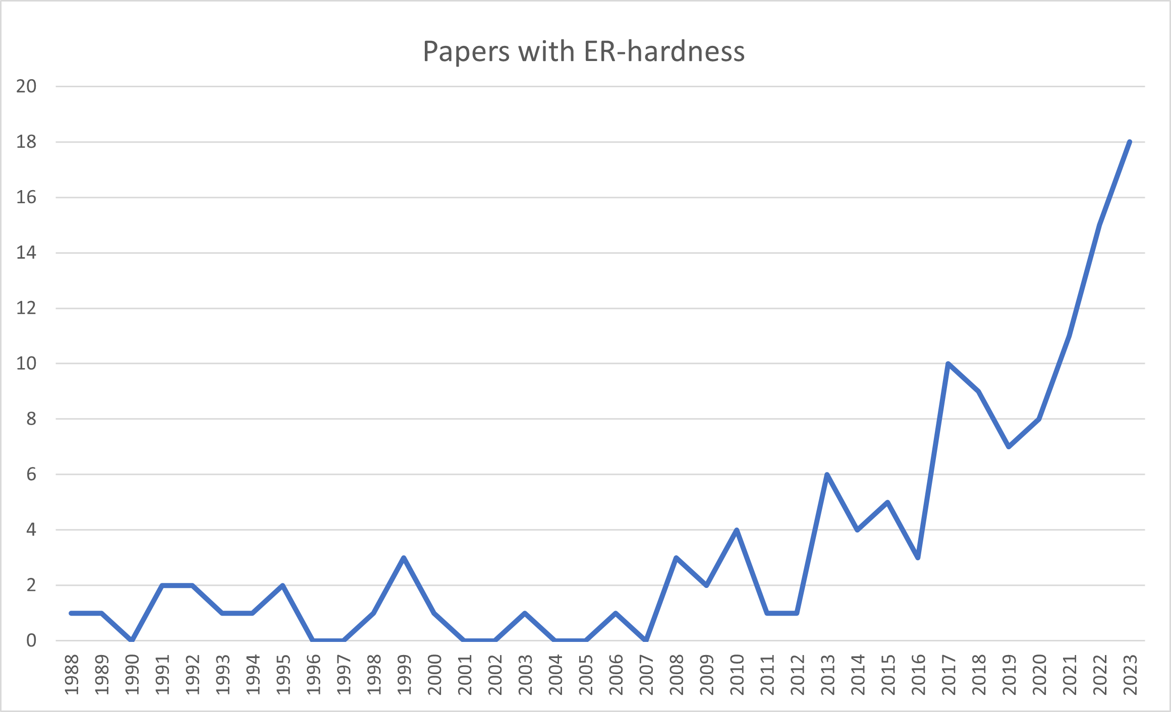
Figure 8: Number of papers with $\exists\mathbb{R}$-hardness results by year.

Computational geometry is by far the most active area for $\exists\mathbb{R}$-complete problems, though we have to admit that the classification of problems is somewhat ambiguous.

Part II A Tour of the Compendium

We give a very brief preview of the compendium and some broader context.

Our compendium collects $\exists\mathbb{R}$-complete problems, but it also goes farther by including $\exists\mathbb{R}$-hard problems, as long as they belong to higher levels of the polynomial hierarchy beyond $\exists\mathbb{R}$, that is, problems that can be captured by the theory of the reals with a bounded number of quantifier alternations.

Within the entries, we will point out related universality results if we are aware of them. As we mentioned, there are many different notions of universality, depending on the equivalence relation that is used. We refer to Verkama [V23c] for a recent discussion on the notion of stable equivalence used by Richter-Gebert [RG96].

We will not discuss problems complete for several other complexity classes that are related to $\exists\mathbb{R}$, but probably different. This includes $\NP^{\mathrm{SSQR}}$, $\P^{\mathrm{SSQR}}$, and $\exists\mathbb{R}\cap\forall\mathbb{R}$—which we already discussed earlier, variants of the BSS computation model, and classes such as FIXP and , which are important in the context of game theory.

We also make no attempt to include problems complete for other existential theories, such as the existential theory of arbitrary rings and fields introduced in [BFS99]. The most interesting are perhaps the existential theory of $\operatorname{GF}(2)$, which yields , $\exists\mathbb{Q}$, whose complexity is still unknown (possibly undecidable) [P09], $\exists\mathbb{N}$, Hilbert’s Tenth problem, which is undecidable by results of Davis, Robinson, and Matiyasevich [M06b], and $\exists\mathbb{C}$ which lies in the second level of the polynomial hierarchy by a result of Koiran’s, assuming the generalized Riemann hypothesis [K97]. However, if natural variants of $\exists\mathbb{R}$-hard problems turn out to be complete for other existential theories, we will mention this fact. For example, $\exists\mathbb{Q}$ is relevant in the field of graph drawing, since it naturally occurs when looking at grid variants of graph drawing problems such as planar slope number, visibility graph, and right-angle crossing drawings, or in rational Nash Equilibria [BH22].

The entries in the compendium are mostly self-contained, though some common notions are defined at the beginning of each section. To keep the entries brief and focused on complexity aspects, we do not include definitions of some of the more intricate notions, relying on references in that case. We include cross-references between related entries.

There are plenty of open problems, both within the entries, and in Section LABEL:sec:Candidates on candidate problems. We have not carefully vetted all papers listed in this compendium, so we cannot guarantee correctness of results. Instead we opted to be inclusive to cover more ground, so we also include preprints; this allows the reader to follow up with the original sources. We will mention issues with papers if we are aware of them.

4 Logic

The existential theory of the reals LABEL:p:ETR, as the name suggests, is anchored in logic, as it is defined by the language ETR, a fragment of the theory of the reals. As we have seen, ETR is a powerful, and expressive language, which makes it useful for upper bounds, but inconvenient for reductions; we would prefer restricted versions of this language, and, as it turns our, $\exists\mathbb{R}$ is quite robust when it comes to the exact definition and signature of the underlying logic. Variants include forcing variables to be distinct LABEL:p:DistETR, or ordered LABEL:p:ETRORV, or allowing them to be approximate LABEL:p:epsETR. Another family of variants looks is based on replacing multiplication with inversion, starting with ETR-INV LABEL:p:ETRINV, and including PLANAR-ETR-INV LABEL:p:PlanarETRINV in which the variable constraint graph is planar, and other nonlinear constraints LABEL:p:CSSP.

These restrictions are useful as intermediate problem for reductions to show that other problems are $\exists\mathbb{R}$-complete.

A number of problems in this section also involve other formal systems such as the collinearity logic LABEL:p:CollLogic the $\mathcal{LR}$-calculus involving left/right orientations of triples of points in the plane LABEL:p:LRCalculus, the region-connection calculus LABEL:p:RCC8con, or Birkhoff and von Neumann’s quantum logic [BvN36] LABEL:p:QuantumStrong,