Recursive Optimal Stopping with Poisson Stopping Constraints

Abstract

This paper solves a recursive optimal stopping problem with Poisson stopping constraints using the penalized backward stochastic differential equation (PBSDE) with jumps. Stopping in this problem is only allowed at Poisson random intervention times, and jumps play a significant role not only through the stopping times but also in the recursive objective functional and model coefficients. To solve the problem, we propose a decomposition method based on Jacod-Pham that allows us to separate the problem into a series of sub-problems between each pair of consecutive Poisson stopping times. To represent the value function of the recursive optimal stopping problem when the initial time falls between two consecutive Poisson stopping times and the generator is concave/convex, we leverage the comparison theorem of BSDEs with jumps. We then apply the representation result to American option pricing in a nonlinear market with Poisson stopping constraints.

60H10, 60G40, 93E20

1 Introduction

The solution of a reflected backward stochastic differential equation (RBSDE) is widely recognized to correspond to the value function of an optimal stopping problem. See [3], [7] and [11] driven by Brownian motion, [8], [12] and [13] involving jumps, and [1], [4], [9] and [32] for the case of $g$-expectations.

However, it is worth noting that a penalized backward stochastic differential equation (PBSDE), often utilized to approximate an RBSDE as the penalization parameter $\lambda$ approaches infinity, also allows for stochastic control representations. Lepeltier and Xu [22] established a connection between the solution of a PBSDE and the value function of a standard optimal stopping problem. In this connection, a modified obstacle $\min\{S_{t},Y_{t}^{\lambda}\}$ depending on the original obstacle $S_{t}$ and the solution $Y_{t}^{\lambda}$ of the PBSDE has been introduced. More relevant to our work, Liang [24] discussed the links between the solution of a PBSDE and the value function of an optimal stopping problem with Poisson stopping constraints. Roughly speaking, he established that the PBSDE (2.5) in Lemma 2.5 admits the following representation:

(1) $$Y_{0}^{\lambda}=\sup_{\tau>0}\mathbb{E}\left[\int_{0}^{\tau\wedge T}f(x,X_{s})\,ds+g(\tau\wedge T,X_{\tau\wedge T})\right],$$

where $\tau$ is selected from an exogenous sequence of Poisson stopping times.

The study of optimal stopping problems with Poisson stopping constraints was initiated by Dupuis and Wang [6] who approached it by solving two ordinary differential equations defined in the continuation and stopping regions. Subsequently, Lempa [21] and Hobson [15] further developed this line of research by considering general one-dimensional diffusions. Liang and Sun [25] extended to Dynkin games with Poisson stopping constraints and investigated optimal conversion and calling strategies for convertible bonds. Hobson and Zeng [14] generalized the exogenous homogeneous Poisson process in Poisson stopping constraints to an inhomogeneous Poisson process, allowing players to choose their intensity with the corresponding costs. Menaldi and Robin examined stopping constraints with independent and identically distributed arrival times for optimal stopping problems in [26] and for optimal impulse control problems in [27] and [28]. Reisinger and Zhang further obtained the convergence rates in [33].

Poisson stopping constraints offer both mathematical generalizations and valuable modeling merits. The underlying Poisson process is utilized to capture external instantaneous impacts on the system, such as credit events. These events result in totally inaccessible jumps within the system. Additionally, Poisson stopping constraints serve as external constraints that determine admissible stopping times for the system to have sufficient liquidity and be allowed to stop. Furthermore, they can be employed to describe information constraints, allowing for the consideration of scenarios where observations are only available at Poisson stopping times. For their applications, see Liang et al. [23] for dynamic bank run problems; Palmowski et al. [29] for optimal capital structure models.

In this paper, we focus on a recursive optimal stopping problem with Poisson stopping constraints, with the objective functional represented by a sequence of possibly nonlinear BSDEs with jumps, stopped by a sequence of Poisson stopping times. The player then selects over Poisson stopping times to maximize their recursive objective functional. Unlike previous studies on nonlinear optimal stopping under $g$-expectation (see [1], [4], [9], and [32]), our model does not require the extra constant preservation assumption on the $g$-expectation. Moreover, while existing results on Poisson stopping constraints typically assume that the objective functional depends solely on Brownian filtration, we demonstrate that including Poisson filtration in the objective functional introduces unexpected complexity. Indeed, when the objective functional is solely based on the Brownian filtration, it results in a conventional penalty term commonly used in PBSDEs. However, when including jumps into the objective functional, this is no longer the case. Our findings shed light on the intricate challenges associated with including jumps in the objective functional of optimal stopping problems with Poisson stopping constraints.

One of the fundamental tools utilized in our analysis is the Jacod-Pham decomposition for optional and predictable processes in the underlying Brownian and Poisson filtration. This filtration assumption allows us to decompose a process, whether it is optional or predictable, into a sequence of processes defined over consecutive Poisson stopping time intervals. Within each interval, the corresponding process depends solely on the jumps up to that point and on the Brownian motion. The Jacod-Pham decomposition, initially proposed by Jacod [16] (see also Jeulin and Yor [17]) has been subsequently applied to solve BSDEs with jumps by Pham [30] (see also Jiao et al. [18], Kharroubi and Lim [19]). Motivated by the Jacod-Pham decomposition, we introduce an update scheme for the penalty term within each Poisson stopping time interval. This scheme involves shifting the value function and the obstacle process forward. By utilizing the representation formula of the jump component of the BSDE solution and introducing a new auxiliary process, we are able to capture and record the differences of the value functions in any two consecutive Poisson stopping time intervals as well as the differences in the obstacle processes within these intervals. By incorporating these elements, we effectively account for the variations and changes that occur across successive Poisson stopping time intervals.

Regarding the generator in the BSDE representation for the recursive objective functional, we first consider the case that the generator is independent of $Z$ and $C$, which are the hedging components of the BSDE solution. In this case, the objective functional is defined recursively using the solution $Y$ of the representing BSDE. The corresponding PBSDE representation for the recursive optimal stopping problem with Poisson stopping constraints has a relatively simple yet interpretable penalty term. This penalty term involves the forward shift of the value function and the obstacle process. However, when the generator depends on $Z$ and $C$, the penalty term takes on an unexpectedly complex form due to the intricacies caused by the Poisson stopping times. In the latter case, we first consider the scenario where the generator depends on $Z$ and $C$ in a linear way. We introduce an adjoint process allowing us to transform the generator in such a way that it no longer relies on $Z$ and $C$. When the generator is concave/convex in $Z$ and $C$, we apply a convex duality argument along with the BSDE comparison with jumps and propose that the corresponding PBSDE representation for the recursive optimal stopping with Poisson stopping constraints should be a limit for a sequence of PBSDEs associated with the linear dependence on $Z$ and $C$.

Many examples of objective functionals fit into our recursive optimal stopping framework. One such example is the pricing of American options, as proposed in [6]. In this case, the generator is linear in $Y$ and $Z$, while remaining independent of $C$. Another example is the stock trading model presented in [2], which is equivalent to the generator that depends solely on $Y$. In the following, we address a comprehensive example in American options that includes all possible cases we investigate in the paper.

Example 1.1 (American option pricing in a nonlinear market with Poisson stopping constraints).

Suppose that a market consists of three securities: a risk-free bond $S^{0}$ and two risky assets $S^{1}$ and $S^{2}$. They evolve according to the following equations

$$dS_{t}^{0} =S_{t}^{0}r_{t}dt,$$

$$dS_{t}^{1} =S_{t}^{1}[\mu_{t}^{1}dt+\sigma_{t}dW_{t}],$$

$$dS_{t}^{2} =S_{t-}^{2}[\mu_{t}^{2}dt+\eta_{t}\tilde{N}(dt)],$$

where $W$ is a standard Brownian Motion, $\tilde{N}$ is the compensated Poisson martingale measure of a Poisson process $N$, and $r_{t}\in\mathbb{R},\mu_{t}^{1}\in\mathbb{R},\mu_{t}^{2}\in\mathbb{R},\sigma_{t}>0$, $\eta_{t}>-1$ are bounded processes predictable to the underling Brownian motion and Poisson process. To exclude arbitrage, we further assume that $\mu_{t}^{2}=0$ when $\eta_{t}=0$. Otherwise, $S^{2}$ becomes another risk-free bond. Furthermore, for technical reasons, we assume that $1/\sigma_{t}$ and $1/\eta_{t}\mathbb{I}_{\{\eta_{t}\neq 0\}}$ are also bounded.

Let $\pi=(\pi^{1},\pi^{2})$ denote the amount of the money invested in the risky assets $(S^{1},S^{2})$. The self-financing strategy leads to a linear equation for the wealth process

(2) $$dV_{t}=\big{[}r_{t}V_{t}+(\mu_{t}^{1}-r_{t}){\pi}_{t}^{1}+(\mu_{t}^{2}-r_{t})\pi_{t}^{2}\big{]}dt+\sigma_{t}\pi_{t}^{1}dW_{t}+\eta_{t}\pi_{t}^{2}\tilde{N}(dt),$$

One may generalize the above linear wealth equation to a general nonlinear case, and use it to replicate an American option with payoff $g(S^{1},S^{2})$ and maturity $T$, exercised at a sequence of Poisson stopping times $\tau$ generated by the Poisson process $N$. It will lead to a sequence of BSDEs with jumps as the objective functional, stopped by a sequence of Poisson stopping times $\tau$:

$$\tilde{Y}_{t}^{\tau}=g({S}^{1}_{\tau\wedge T},{S}^{2}_{\tau\wedge T})+\int_{t\wedge\tau}^{\tau\wedge T}f(s,\tilde{Y}_{s}^{\tau},\tilde{Z}_{s}^{\tau},\tilde{C}_{s}^{\tau})ds-\int_{t\wedge\tau}^{\tau\wedge T}\tilde{Z}_{s}^{\tau}dW_{s}-\int_{t\wedge\tau}^{\tau\wedge T}\tilde{C}_{s}^{\tau}\tilde{N}(ds).$$

The player then selects over the sequence of Poisson stopping times $\tau$ to maximize their recursive objective functional: $\sup_{\tau>0}\tilde{Y}^{\tau}_{0}.$ In the classical linear case, the generator $f$ has the form

$$f(t,y,z,c)=-r_{t}y-\frac{\mu_{t}^{1}-r_{t}}{\sigma_{t}}z-\frac{\mu_{t}^{2}-r_{t}}{\eta_{t}}c\mathbb{I}_{\{\eta_{t}\neq 0\}}$$

according to the linear wealth equation (2).

In this paper, we will discuss general nonlinear cases motivated by American option models in nonlinear markets (see, for example, [5], [10], and [20]). This is driven by the existence of bid-ask spreads for the drifts of the two risky assets and the interest rate of the risk-free bond, which depend on the long-short positions of the two risky assets and the risk-free bond. Specifically, we will assume that $(\mu_{t}^{1},\mu_{t}^{2},r_{t})=(\underline{\mu}^{1}_{t},\underline{\mu}^{2}_{t},\underline{r}_{t})$ for the long positions of the two risky assets and the risk-free bond, and $(\mu_{t}^{1},\mu_{t}^{2},r_{t})=(\overline{\mu}^{1}_{t},\overline{\mu}^{2}_{t},\overline{r}_{t})$ for the short positions. The bounded and predictable processes $\overline{\mu}^{1}_{t}\geq\underline{\mu}^{1}_{t}$, $\overline{\mu}^{2}_{t}\geq\underline{\mu}^{2}_{t}$, and $\overline{r}_{t}\geq\underline{r}_{t}$ represent the bid-ask spreads of the drifts of the two risky assets and the interest rate of the risk-free bond, respectively. Consequently, the linear wealth equation (2) becomes nonlinear:

$$dV_{t}= \big{[}(V_{t}-\pi_{t}^{1}-\pi_{t}^{2})^{+}\underline{r}_{t}-(V_{t}-\pi_{t}^{1}-\pi_{t}^{2})^{-}\overline{r}_{t}\big{]}dt$$

$$+(\pi_{t}^{1})^{+}(\underline{\mu}^{1}_{t}dt+\sigma_{t}dW_{t})-(\pi_{t}^{1})^{-}(\overline{\mu}^{1}_{t}dt+\sigma_{t}dW_{t})$$

$$+(\pi_{t}^{2})^{+}(\underline{\mu}^{2}_{t}dt+\eta_{t}\tilde{N}(dt))-(\pi_{t}^{2})^{-}(\overline{\mu}^{2}_{t}dt+\eta_{t}\tilde{N}(dt))$$

$$= \big{[}\underline{r}_{t}(V_{t}-\pi_{t}^{1}-\pi_{t}^{2})^{+}-\overline{r}_{t}(V_{t}-\pi_{t}^{1}-\pi_{t}^{2})^{-}$$

$$\quad+\underline{\mu}^{1}_{t}(\pi_{t}^{1})^{+}-\overline{\mu}^{1}_{t}(\pi_{t}^{1})^{-}$$

(3) $$\quad+\underline{\mu}^{2}_{t}(\pi_{t}^{2})^{+}-\overline{\mu}^{2}_{t}(\pi_{t}^{2})^{-}\big{]}dt+\sigma_{t}\pi_{t}^{1}dW_{t}+\eta_{t}\pi_{t}^{2}\tilde{N}(dt).$$

It then follows from (1.1) that the generator has the following nonlinear form:

$$f(t,y,z,c)= -\underline{r}_{t}\left(y-\frac{z}{\sigma_{t}}-\frac{c}{\eta_{t}}\mathbb{I}_{\{\eta_{t}\neq 0\}}\right)^{+}+\overline{r}_{t}\left(y-\frac{z}{\sigma_{t}}-\frac{c}{\eta_{t}}\mathbb{I}_{\{\eta_{t}\neq 0\}}\right)^{-}$$

$$-\underline{\mu}^{1}_{t}\frac{z^{+}}{\sigma_{t}}+\overline{\mu}^{1}_{t}\frac{z^{-}}{\sigma_{t}}-\underline{\mu}^{2}_{t}\left(\frac{c}{\eta_{t}}\right)^{+}\mathbb{I}_{\{\eta_{t}\neq 0\}}+\overline{\mu}^{2}_{t}\left(\frac{c}{\eta_{t}}\right)^{-}\mathbb{I}_{\{\eta_{t}\neq 0\}},$$

which is Lipchitz continuous and convex in $(y,z,c)$.

The rest of this paper is organized as the following. Section 2 formulates the recursive optimal stopping problem with Poisson stopping constraints and introduces a class of PBSDEs with jumps as the candidate solutions. Then, we consider the case where the generator is independent of $Z$ and $C$ in Section 3, linear in $Z$ and $C$ in Section 4 and convex in $Z$ and $C$ in Section 5. We apply the representation results to American option pricing in Section 6 and conclude in Section 7.

2 Preliminary Results

In this section, we present the formulation of the recursive optimal stopping problem with Poisson stopping constraints and introduce a class of PBSDEs used to characterize its solution.

Let $\left(\Omega,\mathcal{F},\mathbb{P}\right)$ be a complete probability space supporting a $d$-dimensional standard Brownian motion $W$ with its augmented filtration $\mathbb{F}=\left\{\mathcal{F}_{t}\right\}_{t\geq 0}$. Moreover, let $\left\{T_{i}\right\}_{i\geq 0}$ be the arrival times of an independent Poisson process $N$ with the intensity $\lambda$ and the augmented filtration $\mathbb{H}=\left\{\mathcal{H}_{t}\right\}_{t\geq 0}$. Define $\mathcal{G}_{t}:=\mathcal{F}_{t}\bigvee\mathcal{H}_{t}$ and $\mathbb{G}:=\left(\mathcal{G}_{t}\right)_{t\geq 0}$. Without loss of generality, we assume that $T_{0}=0$ and $T_{\infty}=\infty$. We also use $N:=N(\omega,dt)$ to represent the random jump measure generated by the Poisson process $N$ with the compensator $\hat{N}(dt):=\lambda dt$ such that $\tilde{N}([0,t])=(N-\hat{N})([0,t])$, $t\geq 0$, is a martingale. In the rest of our paper, we will use the following notations:

$$L_{\mathbb{G}}^{2}(0,T;\mathbb{R}^{k}) :=\Big{\{}\varphi:[0,T]\times\Omega\rightarrow\mathbb{R}^{k}\ \Big{|}\ \{\varphi_{t}\}_{0\leq t\leq T}\text{ is }\mathbb{G}\text{-progressively}$$

$$\qquad\quad\text{measurable with }\mathbb{E}\Big{[}\int_{0}^{T}\left|\varphi_{t}\right|^{2}dt\Big{]}<+\infty\Big{\}},$$

$$L_{\mathbb{G}}^{2,p}(0,T;\mathbb{R}^{k}) :=\Big{\{}\varphi:[0,T]\times\Omega\rightarrow\mathbb{R}^{k}\ \Bigg{|}\ \{\varphi_{t}\}_{0\leq t\leq T}\text{ is }\mathbb{G}\text{-predictable with }$$

$$\qquad\quad\mathbb{E}\Big{[}\int_{0}^{T}\left|\varphi_{t}\right|^{2}dt\Big{]}<+\infty\Big{\}},$$

$$S_{\mathbb{G}}^{2}(0,T;\mathbb{R}^{k}) :=\Big{\{}\varphi:[0,T]\times\Omega\rightarrow\mathbb{R}^{k}\ \Big{|}\ \{\varphi_{t}\}_{0\leq t\leq T}\text{ is }\mathbb{G}\text{-adapted with}$$

$$\qquad\quad\text{c\`{a}dl\`{a}g sample paths and }\mathbb{E}\Big{[}\sup_{0\leq t\leq T}\left|\varphi_{t}\right|^{2}\Big{]}<+\infty\Big{\}},$$

$$\mathcal{T} :=\Big{\{}\tau:\Omega\rightarrow[0,T]\ \Big{|}\ \tau\text{ is a $\mathbb{G}$-stopping time}\Big{\}},$$

$$\mathbb{I}_{t}^{i} :=\mathbb{I}_{\{T_{i-1}\leq t<T_{i}\}},\quad i\geq 1.$$

2.1 Recursive Optimal Stopping Problem with Poisson Stopping Constraints

To start with, we introduce the admissible stopping set starting at $T_{i}$ as

$$\mathcal{R}_{T_{i}}(\lambda):=\left\{\left.\tau\in\mathcal{T}\,\right|\,\text{for any }\omega\in\Omega,\,\tau(\omega)=T_{n}(\omega)\wedge T\text{, where }n\geq i\right\},\$$

and the admissible stopping set starting at time $t$, which may not necessarily be a jump time, as

$$\mathcal{R}_{t}(\lambda):=\left\{\left.\tau\in\mathcal{T}\,\right|\,\text{for any }\omega\in\Omega,\,\tau(\omega)=T_{n}(\omega)\wedge T\geq t\text{, where }n\geq 0\right\}.$$

For $\mathcal{R}_{t+}(\lambda)$, we require $\tau(\omega)=T_{n}(\omega)\wedge T>t$ instead. Moreover, for $\tau\in\mathcal{R}_{t+}(\lambda)$, we introduce the following BSDE with jumps as a recursive objective functional: for $t\in[0,T]$,

$$\left\{\begin{aligned} {X}_{t}&=x+\int_{0}^{t}b(s,{X}_{s})ds+\int_{0}^{t}\sigma(s,{X}_{s})dW_{s}+\int_{0}^{t}h(s,{X}_{s-})\tilde{N}(ds),\\ \tilde{Y}_{t}^{\tau}&={g({\tau},{X}_{\tau})}+\int_{t}^{\tau}f(s,{X}_{s},\tilde{Y}_{s}^{\tau},\tilde{Z}_{s}^{\tau},\tilde{C}_{s}^{\tau})ds\\ &\qquad-\int_{t}^{\tau}\tilde{Z}_{s}^{\tau}dW_{s}-\int_{t}^{\tau}\tilde{C}_{s}^{\tau}\tilde{N}(ds).\end{aligned}$$

In addition, the coefficients $b\left(t,x\right):\Omega\times\left[0,T\right]\times\mathbb{R}^{n}\rightarrow\mathbb{R}^{n}$, $\sigma\left(t,x\right):\Omega\times\left[0,T\right]\times\mathbb{R}^{n}\rightarrow\mathbb{R}^{n\times d}$, $h\left(t,x\right):\Omega\times\left[0,T\right]\times\mathbb{R}^{n}\rightarrow\mathbb{R}^{n}$, $g\left(t,x\right):\Omega\times\left[0,T\right]\times\mathbb{R}^{n}\rightarrow\mathbb{R}$ and $f\left(t,x,y,z,c\right):\Omega\times\left[0,T\right]\times\mathbb{R}^{n}\times\mathbb{R}\times\mathbb{R}^{d}\times\mathbb{R}\rightarrow\mathbb{R}$ satisfy the following assumptions. The coefficients $b(\cdot,x)\in L_{\mathbb{G}}^{2}(0,T;\mathbb{R}^{n}),\,\sigma(\cdot,x)\in L_{\mathbb{G}}^{2}(0,T;\mathbb{R}^{n\times d})$ and $h(\cdot,x)\in L_{\mathbb{G}}^{2,p}(0,T;\mathbb{R}^{n})$ for any $x\in\mathbb{R}^{n}$, and there exists a constant $L>0$ such that for any $t\in[0,T]$, $x$ and $x^{\prime}\in\mathbb{R}^{n}$,

$$\left|b\left(t,x\right)\right|+\left|\sigma\left(t,x\right)\right|+\left|h\left(t,x\right)\right| \leq L\left(1+|x|\right),$$

$$\left|b\left(t,x\right)-b\left(t,x^{\prime}\right)\right|+\left|\sigma\left(t,x\right)-\sigma\left(t,x^{\prime}\right)\right|+\left|h\left(t,x\right)-h\left(t,x^{\prime}\right)\right| \leq L\left|x-x^{\prime}\right|.$$

The generator $f(\cdot,x,y,z,c)\in L_{\mathbb{G}}^{2}(0,T;\mathbb{R})$, the obstacle process $g(\cdot,x)\in S_{\mathbb{G}}^{2}(0,T;\mathbb{R})$ for any $(x,y,z,c)\in\mathbb{R}^{n}\times\mathbb{R}\times\mathbb{R}^{d}\times\mathbb{R}$, and there exists a constant $L>0$ such that for any $t\in[0,T]$, $(x,y,z,c)$ and $(x^{\prime},y^{\prime},z^{\prime},c^{\prime})\in\mathbb{R}^{n}\times\mathbb{R}\times\mathbb{R}^{d}\times\mathbb{R}$,

$$\left|g\left(t,x\right)\right|\leq L(1+|x|),\qquad\left|g\left(t,x\right)-g\left(t,x^{\prime}\right)\right|\leq L\left|x-x^{\prime}\right|,$$

$$\left|f\left(t,x,y,z,c\right)\right|\leq L\left(1+|x|+|y|+|z|\right),$$

$$\left|f\left(t,x,y,z,c\right)-f\left(t,x^{\prime},y^{\prime},z^{\prime},c^{\prime}\right)\right|\leq L\left(\left|x-x^{\prime}\right|+\left|y-y^{\prime}\right|+\left|z-z^{\prime}\right|+\left|c-c^{\prime}\right|\right).$$

The solvability of (2.1) can be obtained under the above assumptions according to [34, Theorem 2.1].

Lemma 2.1.

Suppose that Sections 2.1 and 2.1 hold. The BSDE with jumps (2.1) admits a unique adapted solution $({X},\tilde{Y}^{\tau},\tilde{Z}^{\tau},\tilde{C}^{\tau})\in S_{\mathbb{G}}^{2}(0,T;\mathbb{R}^{n})\times S_{\mathbb{G}}^{2}(0,T;\mathbb{R})\times L_{\mathbb{G}}^{2,p}(0,T;\mathbb{R}^{d})\times L_{\mathbb{G}}^{2,p}(0,T;\mathbb{R})$.

The BSDE with jumps (2.1) requires an additional condition, as stated in [34, Theorem 4.1] and [31, Theorem 4.4], in order to restrict the magnitude of the jumps and ensure that the comparison theorem holds. For any $(t,y,z)\in[0,T]\times\mathbb{R}\times\mathbb{R}^{d},\,c$ and $c^{\prime}\in\mathbb{R}$ with $c\neq c^{\prime}$,

(4) $$\frac{f(t,X_{t},y,z,c)-f(t,X_{t},y,z,c^{\prime})}{\lambda(c-c^{\prime})}\geq-1.$$

The recursive objective functional of the optimal stopping problem with Poisson stopping constraints is given by (2.1). Then, we propose the following optimal stopping problem.

Problem 2.2 (Recursive optimal stopping problem with Poisson stopping constraints).

Suppose that Sections 2.1, 2.1, and 2.1 hold. We aim to find an admissible stopping time $\hat{\tau}^{*}\in\mathcal{R}_{T_{1}}(\lambda)$ to maximize the recursive objective functional given by (2.1), such that

$$V^{\lambda}_{0}:=\sup_{\tau\in\mathcal{R}_{T_{1}}(\lambda)}\tilde{Y}_{0}^{\tau}=\tilde{Y}_{0}^{\hat{\tau}^{*}}.$$

In general, $V_{t}^{\lambda}$ is defined as the value function of the optimal stopping problem

$$V^{\lambda}_{t}:=\sup_{\tau\in\mathcal{R}_{T_{i}}(\lambda)}\tilde{Y}_{t}^{\tau}=\tilde{Y}_{t}^{\hat{\tau}^{*}_{t}},\quad\text{conditional on }\big{\{}T_{i-1}\leq t<T_{i}\big{\}},\quad i\geq 1,$$

with the optimal stopping time denoted as $\hat{\tau}_{t}^{*}$.

Note that $V^{\lambda}_{t}=\sup_{\tau\in\mathcal{R}_{t+}(\lambda)}\tilde{Y}_{t}^{\tau}$ for $t\in[0,T)$ and, in particular, when $t=0,$ $\tau\geq T_{1}$, so the system is not allowed to stop at initial time $0$.

2.2 PBSDE with Jumps

In the following, we introduce a new PBSDE with jumps which will be utilized to solve 2.2, namely, for $t\in[0,T]$,

(5) $$\begin{aligned} \hat{Y}_{t}^{\lambda}&=g({T},{X}_{T})+\int_{t}^{T}\Big{[}f\Big{(}s,{X}_{s},\hat{Y}_{s}^{\lambda},\hat{Z}_{s}^{\lambda},\hat{C}_{s}^{\lambda}+\Big{(}g(s,{X}_{s})+A_{s}-\hat{Y}_{s}^{\lambda}-\hat{C}_{s}^{\lambda}\Big{)}^{+}\Big{)}\\ &\qquad+\lambda\Big{(}g(s,{X}_{s})+A_{s}-\hat{Y}_{s}^{\lambda}-\hat{C}_{s}^{\lambda}\Big{)}^{+}\Big{]}ds-\int_{t}^{T}\hat{Z}_{s}^{\lambda}dW_{s}-\int_{t}^{T}\hat{C}_{s}^{\lambda}\tilde{N}(ds),\end{aligned}$$

where $A\in L_{\mathbb{G}}^{2}(0,T;\mathbb{R})$ is an auxiliary process used to record the difference of $g(t,{X}_{t})$ in $[T_{i-1},T_{i})$ and $[T_{i},T_{i+1})$ for $i\geq 1$. More specifically, we introduce (Poisson) time indexes

$$\begin{aligned} T_{(i)}&:=(T_{1},\cdots,T_{i}),\quad i\geq 1,\\ \Delta_{i}&:=\left\{\theta_{(i)}:=(\theta_{1},\cdots,\theta_{i})\in\mathbb{R}^{i}\left|\theta_{1}\leq\theta_{2}\leq\cdots\leq\theta_{i}\right.\right\},\quad i\geq 1.\end{aligned}$$

We also write $T_{(i)}=(T_{(i-1)},T_{i})$ and $\theta_{(i)}=(\theta_{(i-1)},\theta_{i})$. Then, the Jacod-Pham decomposition for optional processes (see [16], [17] and more recently [30]) implies that

$$g(t,{X}_{t})=\sum_{i\geq 0}g^{i}(t,T_{(i)})\mathbb{I}_{t}^{i+1},$$

where $g^{i}(\cdot,\theta_{(i)})\in L_{\mathbb{F}}^{2}(0,T;\mathbb{R})$ for any $\theta_{(i)}\in\Delta_{i}$. In turn, the auxiliary process $A$ is defined as with ${A}^{i}(t,T_{(i)}):={A}^{i}(t,\theta_{(i)})|_{\theta_{(i)}=T_{(i)}}$ given by

$${A}^{i}(t,\theta_{(i)}):=g^{i+1}(t,(\theta_{(i)},t))-g^{i}(t,\theta_{(i)}),\quad i\geq 0.$$

It is evident that when the generator $f$ satisfies Assumption 2.1, the generator of PBSDE (5) also satisfies the same assumption. Following the result in [34, Theorem 2.1], we have:

Lemma 2.3.

Suppose that Sections 2.1 and 2.1 hold. Then, the PBSDE with jumps (5) admits a unique adapted solution $(\hat{Y}^{\lambda},\hat{Z}^{\lambda},\hat{C}^{\lambda})\in S_{\mathbb{G}}^{2}(0,T;\mathbb{R})\times L_{\mathbb{G}}^{2,p}(0,T;\mathbb{R}^{d})\times L_{\mathbb{G}}^{2,p}(0,T;\mathbb{R})$.

In addition, note that if the generator $f$ satisfies Assumption 2.1, then the generator of (5) also satisfies the same assumption. In other words, for any $(t,y,z)\in[0,T]\times\mathbb{R}\times\mathbb{R}^{d},\,c$ and $c^{\prime}\in\mathbb{R}$ with $c\neq c^{\prime}$, the generator meets the requirements of Assumption 2.1:

$$\begin{aligned} &\frac{f(t,X_{t},y,z,c+(g(t,X_{t})+A_{t}-y-c)^{+})+\lambda(g(t,X_{t})+A_{t}-y-c)^{+}}{\lambda(c-c^{\prime})}\\ &-\frac{f(t,X_{t},y,z,c^{\prime}+(g(t,X_{t})+A_{t}-y-c^{\prime})^{+})+\lambda(g(t,X_{t})+A_{t}-y-c^{\prime})^{+})}{\lambda(c-c^{\prime})}\geq-1,\end{aligned}$$

so the comparison theorem also holds for (5).

2.3 Decomposition for PBSDE with jumps

This part provides a decomposition result for the coefficients and the solution of the PBSDE with jumps (5), which plays an important role in deriving its representation for the value function $V^{\lambda}_{t}$ of 2.2. The decomposition result will also be used to obtain the recursive equation in Lemma 3.4 in the next section.

First, by employing the definition of the martingale measure $\tilde{N}$, we can establish the equivalence of (5) with the following equation:

$$\begin{aligned} \hat{Y}_{t}^{\lambda}&=g({T},{X}_{T})+\int_{t}^{T}f\Big{(}s,{X}_{s},\hat{Y}_{s}^{\lambda},\hat{Z}_{s}^{\lambda},\hat{C}_{s}^{\lambda}+\Big{(}g(s,{X}_{s})+A_{s}-\hat{Y}_{s}^{\lambda}-\hat{C}_{s}^{\lambda}\Big{)}^{+}\Big{)}ds\\ &\qquad+\int_{t}^{T}\lambda\max\Big{\{}g(s,{X}_{s})+A_{s}-\hat{Y}_{s}^{\lambda},\hat{C}_{s}^{\lambda}\Big{\}}ds-\int_{t}^{T}\hat{Z}_{s}^{\lambda}dW_{s}-\int_{t}^{T}\hat{C}_{s}^{\lambda}{N}(ds).\end{aligned}$$

Apply the Jacod-Pham decomposition to the generator (with its càdlàg modification) of the above PBSDE , we obtain

$$f\Big{(}t,{X}_{t},y,z,c+\Big{(}g(t,X_{t})+A_{t}-y-c\Big{)}^{+}\Big{)}+\lambda\max\Big{\{}g(t,{X}_{t})+A_{t}-y,c\Big{\}}$$

$$=\sum_{i\geq 0}h^{i,\lambda}(t,y,z,c,T_{(i)})\mathbb{I}_{t}^{i+1},$$

where $h^{i,\lambda}(\cdot,y,z,c,\theta_{(i)})\in L_{\mathbb{F}}^{2}(0,T;\mathbb{R})$ for any $(y,z,c,\theta_{(i)})\in\mathbb{R}\times\mathbb{R}^{d}\times\mathbb{R}\times\Delta_{i}$. Then, PBSDE (5) admits the following decomposition.

Theorem 2.4.

The solution $(\hat{Y}^{\lambda},\hat{Z}^{\lambda},\hat{C}^{\lambda})$ of the PBSDE with jumps (5) has the following representation for any $t\in[0,T]$:

$$\hat{Y}^{\lambda}_{t} =\sum_{i\geq 0}\hat{Y}^{i,\lambda}_{t}(T_{(i)})\mathbb{I}_{t}^{i+1},$$

$$\hat{Z}^{\lambda}_{t} =\hat{Z}^{0,\lambda}_{t}\mathbb{I}_{\{t\leq T_{1}\}}+\sum_{i\geq 1}\hat{Z}^{i,\lambda}_{t}(T_{(i)})\mathbb{I}_{\{T_{i}<t\leq T_{i+1}\}},$$

$$\hat{C}^{\lambda}_{t} =\hat{C}^{0,\lambda}_{t}\mathbb{I}_{\{t\leq T_{1}\}}+\sum_{i\geq 1}\hat{C}^{i,\lambda}_{t}(T_{(i)})\mathbb{I}_{\{T_{i}<t\leq T_{i+1}\}},$$

with the processes

$$\hat{Y}^{i,\lambda}_{t}(T_{(i)}) :=\hat{Y}^{i,\lambda}_{t}(\theta_{(i)})|_{\theta_{(i)}=T_{(i)}},$$

$$\hat{Z}^{i,\lambda}_{t}(T_{(i)}) :=\hat{Z}^{i,\lambda}_{t}(\theta_{(i)})|_{\theta_{(i)}=T_{(i)}},$$

$$\hat{C}^{i,\lambda}_{t}(T_{(i)}) :=\hat{C}^{i,\lambda}_{t}(\theta_{(i)})|_{\theta_{(i)}=T_{(i)}},$$

given by the following Brownian motion driven BSDE in the time horizon $[\theta_{i}\wedge T,T]$ with $\hat{C}_{t}^{i,\lambda}(\theta_{(i)}):=\hat{Y}_{t}^{i+1,\lambda}((\theta_{(i)},t))-\hat{Y}_{t}^{i,\lambda}(\theta_{(i)})$ for $i\geq 0$:

$$\begin{aligned} \hat{Y}_{t}^{i,\lambda}(\theta_{(i)})&=g^{i}(T,\theta_{(i)})+\int_{t}^{T}{h}^{i,\lambda}(s,\hat{Y}_{s}^{i,\lambda}(\theta_{(i)}),\hat{Z}_{s}^{i,\lambda}(\theta_{(i)}),\hat{C}_{s}^{i,\lambda}(\theta_{(i)}),\theta_{(i)})ds\\ &\qquad-\int_{t}^{T}\hat{Z}_{s}^{i,\lambda}(\theta_{(i)})dW_{s}.\end{aligned}$$

Remark 2.5.

When $f(t,x,y,z,c)=f(t,x)$, $h(t,x)=0$ and all the coefficients in (2.1) are $\mathbb{F}$-adapted, the solution ${X}$ of the forward equation in (2.1) will be $\mathbb{F}$-adapted and the Jacod-Pham decomposition of $g(t,{X}_{t})$ will be trivial with $g^{i}(t,\theta_{(i)})=g(t,{X}_{t})$. Then, (5) degenerates to a standard PBSDE on $\left(\Omega,\mathcal{F},\mathbb{F},\mathbb{P}\right)$, namely,

Remark 2.6.

Unless there are only a finite number of jumps as considered in [30], [18], and [19], so one can solve the sequence of Brownian motion driven BSDEs recursively in a backward way, the Jacod-Pham decomposition in Theorem 2.4 does not help to solve the PBSDE with jumps (5), as the sequence of Brownian motion driven BSDEs is not a closed system therein. Instead, the solvability of (5) is provided in Lemma 2.3, and we will utilize the Jacod-Pham decomposition to establish the connection between (5) and the recursive optimal stopping problem 2.2.

3 Representation for the Case with Generator Independent of $Z$ and $C$

In this section, we study 2.2 when the generator of the recursive objective functional (2.1) is independent of the hedging processes $Z$ and $C$, i.e. $f(t,x,y,z,c)=f(t,x,y)$. In such a case, PBSDE (5) simplifies to the following form:

(6) $$\begin{aligned} \hat{Y}_{t}^{\lambda}&=g({T},{X}_{T})+\int_{t}^{T}\Big{[}f(s,{X}_{s},\hat{Y}_{s}^{\lambda})+\lambda\left(g(s,{X}_{s})+{A}_{s}-\hat{Y}_{s}^{\lambda}-\hat{C}_{s}^{\lambda}\right)^{+}\Big{]}ds\\ &\qquad-\int_{t}^{T}\hat{Z}_{s}^{\lambda}dW_{s}-\int_{t}^{T}\hat{C}_{s}^{\lambda}\tilde{N}(ds),\quad t\in[0,T].\end{aligned}$$

Theorem 3.1.

Suppose that Sections 2.1, 2.1, and 2.1 hold and the generator $f(t,x,y,z,c)=f(t,x,y)$. Then, the value function of 2.2 is given by

(7) $$V^{\lambda}_{t}=\hat{Y}_{t}^{\lambda}=\sup_{\tau\in\mathcal{R}_{T_{i}}(\lambda)}\tilde{Y}_{t}^{\tau},\quad\text{conditional on }\{T_{i-1}\leq t<T_{i}\},\quad i\geq 1,$$

where $\hat{Y}^{\lambda}$ and $\tilde{Y}^{\tau}$ are the unique solutions of (6) and (2.1), respectively. Moreover, the optimal stopping time is given by

(8) $$\hat{\tau}^{*}_{t}:=\inf\Big{\{}T_{n}>t\,\Big{|}\,\hat{Y}^{\lambda}_{T_{n}}\leq g(T_{n},{X}_{T_{n}})\Big{\}}\wedge T.$$

Remark 3.2.

By partitioning the sample space $\Omega$ using the Poisson stopping times $\{T_{i}\}_{i\geq 0}$, we can deduce that

$$\hat{Y}_{t}^{\lambda}=\sum_{i\geq 1}\mathbb{I}_{t}^{i}\hat{Y}_{t}^{\lambda}=\sum_{i\geq 1}\mathbb{I}_{t}^{i}\sup_{\tau\in\mathcal{R}_{T_{i}}(\lambda)}\tilde{Y}_{t}^{\tau},$$

Furthermore, the representation (7) can be expressed more concisely using $\mathcal{R}_{t+}(\lambda)$:

$$\hat{Y}_{t}^{\lambda}=\sup_{\tau\in\mathcal{R}_{t+}(\lambda)}\tilde{Y}_{t}^{\tau},\quad t\in[0,T).$$

Remark 3.3.

If we make the additional assumption that $f(t,x,y)$ is $\mathbb{F}$-adapted and satisfies the remaining conditions stated in Remark 2.5, Theorem 3.1 yields the following result, consistent with [24, Theorem 1.2]:

$${Y}_{t}^{\lambda}=\sup_{\tau\in\mathcal{R}_{T_{i}}(\lambda)}\tilde{Y}_{t}^{\tau},\quad\text{conditional on }\{T_{i-1}\leq t<T_{i}\},\quad i\geq 1,$$

where $({Y}^{\lambda},{Z}^{\lambda})$ is the unique solution of (2.5).

The proof of Theorem 3.1 relies on two key lemmas.

Lemma 3.4.

Suppose that Sections 2.1, 2.1, and 2.1 hold. Then, the process $\hat{Y}^{\lambda}$ given by (6) is the unique solution of the recursive equation

(9) $$\begin{aligned} \hat{Y}^{\lambda}_{t}&=\sum_{i\geq 1}\mathbb{I}_{t}^{i}\cdot\mathbb{E}\Bigg{[}\int_{t}^{T_{i}\wedge T}f(s,{X}_{s},\hat{Y}^{\lambda}_{s})ds+g(T,{X}_{T})\mathbb{I}_{\{T_{i}>T\}}\\ &\qquad+\max\Big{\{}g(T_{i},{X}_{T_{i}}),\hat{Y}^{\lambda}_{T_{i}}\Big{\}}\mathbb{I}_{\{T_{i}\leq T\}}\Bigg{|}\mathcal{G}_{t}\Bigg{]}.\end{aligned}$$

Proof 3.5.

By noting that $\lambda\Big{(}g(t,X_{t})+A_{t}-y-c\Big{)}^{+}=\lambda\max\Big{\{}g(t,X_{t})+A_{t},y+c\Big{\}}-\lambda\big{(}y+c\big{)}$, and applying the Jacod-Pham decomposition to the generator of PBSDE (6) (with its càdlàg modification), we obtain

$$\begin{aligned} f(t,{X}_{t},y)&=\sum_{i\geq 0}f^{i,d}(t,y,T_{(i)})\mathbb{I}_{t}^{i+1},\\ \lambda\max\Big{\{}g(t,{X}_{t})+{A}_{t},y+c\Big{\}}&=\sum_{i\geq 0}\lambda\max\Big{\{}\big{(}g^{i}(t,T_{(i)})+{A}^{i}(t,T_{(i)}),y+c\Big{\}}\mathbb{I}_{t}^{i+1},\end{aligned}$$

where the processes $f^{i,d}(\cdot,\theta_{(i)})$, $K^{i,d}(\cdot,\theta_{(i)})$ $\in L_{\mathbb{F}}^{2}(0,T;\mathbb{R})$ for any $\theta_{(i)}\in\Delta_{i}$. Hence, we obtain the decomposition according to Theorem 2.4: for any $t\in[0,T]$,

(10) $$\begin{aligned} \hat{Y}^{\lambda}_{t}&=\sum_{i\geq 0}\hat{Y}^{i,d}_{t}(T_{(i)})\mathbb{I}_{t}^{i+1},\\ \hat{Z}^{\lambda}_{t}&=\hat{Z}^{0,d}_{t}\mathbb{I}_{\{t\leq T_{1}\}}+\sum_{i\geq 1}\hat{Z}^{i,d}_{t}(T_{(i)})\mathbb{I}_{\{T_{i}<t\leq T_{i+1}\}},\\ \hat{C}^{\lambda}_{t}&=\hat{C}^{0,d}_{t}\mathbb{I}_{\{t\leq T_{1}\}}+\sum_{i\geq 1}\hat{C}^{i,d}_{t}(T_{(i)})\mathbb{I}_{\{T_{i}<t\leq T_{i+1}\}},\end{aligned}$$

with the processes

$$\hat{Y}^{i,d}_{t}(T_{(i)}) :=\hat{Y}^{i,d}_{t}(\theta_{(i)})|_{\theta_{(i)}=T_{(i)}},$$

$$\hat{Z}^{i,d}_{t}(T_{(i)}) :=\hat{Z}^{i,d}_{t}(\theta_{(i)})|_{\theta_{(i)}=T_{(i)}},$$

$$\hat{C}^{i,d}_{t}(T_{(i)}) :=\hat{C}^{i,d}_{t}(\theta_{(i)})|_{\theta_{(i)}=T_{(i)}},$$

given by the following Brownian motion driven BSDE in the time horizon $[\theta_{i}\wedge T,T]$ with $\hat{C}_{s}^{i,d}(\theta_{(i)}):=\hat{Y}_{s}^{i+1,d}((\theta_{(i)},s))-\hat{Y}_{s}^{i,d}(\theta_{(i)})$ for $i\geq 0$:

$$\begin{aligned} \hat{Y}_{t}^{i,d}(\theta_{(i)})&=g^{i}(T,\theta_{(i)})+\int_{t}^{T}\Big{[}f^{i,d}(s,\theta_{(i)})+\lambda\Big{(}g^{i}(s,\theta_{(i)})+{A}^{i}(s,\theta_{(i)})\\ &\qquad-\hat{Y}_{s}^{i,d}(\theta_{(i)})-\hat{C}_{s}^{i,d}(\theta_{(i)})\Big{)}^{+}+\lambda\hat{C}_{s}^{i,d}(\theta_{(i)})\Big{]}ds-\int_{t}^{T}\hat{Z}_{s}^{i,\lambda}(\theta_{(i)})dW_{s}.\end{aligned}$$

Applying Itô’s formula to $e^{-\lambda t}\hat{Y}_{t}^{i,d}(\theta_{(i)})$, we obtain

$$\begin{aligned} e^{-\lambda t}\hat{Y}_{t}^{i,d}(\theta_{(i)})&=e^{-\lambda T}g^{i}(T,\theta_{(i)})+\int_{t}^{T}e^{-\lambda s}\Big{[}f^{i,d}(s,\theta_{(i)})+\lambda\max\Big{\{}g^{i}(s,\theta_{(i)})\\ &\qquad+{A}^{i}(s,\theta_{(i)}),\hat{Y}_{s}^{i,d}(\theta_{(i)})+\hat{C}_{s}^{i,d}(\theta_{(i)})\Big{\}}\Big{]}ds-\int_{t}^{T}e^{-\lambda s}\hat{Z}_{s}^{i,\lambda}(\theta_{(i)})dW_{s}.\end{aligned}$$

Then, it follows that

$$\begin{aligned} \hat{Y}_{t}^{i,d}(\theta_{(i)})&=e^{-\lambda(T-t)}g^{i}(T,\theta_{(i)})+\int_{t}^{T}e^{-\lambda(s-t)}\Big{[}f^{i,d}(s,\theta_{(i)})+\lambda\max\Big{\{}g^{i}(s,\theta_{(i)})\\ &\qquad+{A}^{i}(s,\theta_{(i)}),\hat{Y}_{s}^{i,d}(\theta_{(i)})+\hat{C}_{s}^{i,d}(\theta_{(i)})\Big{\}}\Big{]}ds-\int_{t}^{T}e^{-\lambda(s-t)}\hat{Z}_{s}^{i,\lambda}(\theta_{(i)})dW_{s}.\end{aligned}$$

Taking conditional expectation with respect to $\mathcal{F}_{t}$ on both sides and substituting it into (10), we obtain

(11) $$\begin{aligned} \hat{Y}^{\lambda}_{t}&=\sum_{i\geq 1}\mathbb{I}_{t}^{i}\cdot\mathbb{E}\Bigg{[}e^{-\lambda(T-t)}g^{i-1}(T,\theta_{(i-1)})+\int_{t}^{T}e^{-\lambda(s-t)}\Big{[}f^{i-1,d}(s,\theta_{(i-1)})\\ &\qquad+\lambda\max\Big{\{}g^{i}(s,(\theta_{(i-1)},s)),\hat{Y}_{s}^{i,d}((\theta_{(i-1)},s))\Big{\}}\Big{]}ds\Bigg{|}\mathcal{F}_{t}\Bigg{]}\Bigg{|}_{\theta_{(i-1)}=T_{(i-1)}}.\end{aligned}$$

To derive the recursive equation (9), we apply the Jacod-Pham decomposition to each term on its right hand side and obtain

$$\begin{aligned} \Theta_{1}:=&\,\mathbb{I}_{t}^{i}\cdot\mathbb{E}\Bigg{[}g(T,{X}_{T})\mathbb{I}_{\{T_{i}>T\}}+\max\Big{\{}g(T_{i},{X}_{T_{i}}),\hat{Y}_{T_{i}}^{\lambda}\Big{\}}\mathbb{I}_{\{T_{i}\leq T\}}\Bigg{|}\mathcal{G}_{t}\Bigg{]}\\ =&\,\mathbb{I}_{t}^{i}\cdot\mathbb{E}\Bigg{[}\mathbb{I}_{\{T_{i}>T\}}\sum_{j\geq 1}g^{j-1}(T,T_{(j-1)})\mathbb{I}_{T}^{j}+\mathbb{I}_{\{T_{i}\leq T\}}\sum_{j\geq 1}\max\Big{\{}g^{j-1}(T_{i},T_{(j-1)}),\\ &\,\quad\quad\hat{Y}_{T_{i}}^{j-1,d}(T_{(j-1)})\Big{\}}\mathbb{I}_{T_{i}}^{j}\Bigg{|}\mathcal{G}_{t}\Bigg{]}\\ =&\,\mathbb{E}\Bigg{[}\mathbb{I}_{\{T_{i}>T\}}g^{i-1}(T,T_{(i-1)})\mathbb{I}_{T}^{i}\mathbb{I}_{t}^{i}+\mathbb{I}_{t}^{i}\mathbb{I}_{\{T_{i}\leq T\}}\max\Big{\{}g^{i}(T_{i},T_{(i)}),\hat{Y}_{T_{i}}^{i,d}(T_{(i)})\Big{\}}\mathbb{I}_{T_{i}}^{i+1}\Bigg{|}\mathcal{G}_{t}\Bigg{]}.\end{aligned}$$

Observing that the random variable $\mathbb{I}_{t}^{i}T_{(i-1)}$ is $\mathcal{G}_{t}$-measurable, it follows that

$$\begin{aligned} \Theta_{1}=&\,\mathbb{I}_{t}^{i}\cdot\mathbb{E}\Bigg{[}\mathbb{I}_{\{T_{i}>T\}}g^{i-1}(T,\theta_{(i-1)})\mathbb{I}_{\{\theta_{i-1}\leq t<T_{i}\}}+\mathbb{I}_{\{T_{i}\leq T\}}\max\Big{\{}g^{i}(T_{i},(\theta_{(i-1)},T_{i})),\\ &\,\quad\quad\hat{Y}_{T_{i}}^{i,d}((\theta_{(i-1)},T_{i}))\Big{\}}\mathbb{I}_{\{\theta_{i-1}\leq t<T_{i}\}}\Bigg{|}\mathcal{G}_{t}\Bigg{]}\Bigg{|}_{\theta_{(i-1)}=T_{(i-1)}}.\end{aligned}$$

Similar to [24, Lemma 2.1], we use the conditional density of $T_{i}-t$ conditional on $\{T_{i-1}\leq t<T_{i}\}$ and obtain

(12) $$\begin{aligned} \Theta_{1}=&\,\frac{\mathbb{I}_{t}^{i}}{\mathbb{E}\big{[}\mathbb{I}_{t}^{i}\big{|}\mathcal{F}_{t}\big{]}}\cdot\mathbb{E}\Bigg{[}\mathbb{I}_{\{T_{i}>T\}}g^{i-1}(T,\theta_{(i-1)})+\mathbb{I}_{\{T_{i}\leq T\}}\max\Big{\{}g^{i}(T_{i},(\theta_{(i-1)},T_{i})),\\ &\,\quad\quad\hat{Y}_{T_{i}}^{i,d}((\theta_{(i-1)},T_{i}))\Big{\}}\mathbb{I}_{\{\theta_{i-1}\leq t<T_{i}\}}\Bigg{|}\mathcal{F}_{t}\Bigg{]}\Bigg{|}_{\theta_{(i-1)}=T_{(i-1)}}\\ =&\,\mathbb{I}_{t}^{i}\cdot\mathbb{E}\Bigg{[}e^{-\lambda(T-t)}g^{i-1}(T,\theta_{(i-1)})+\int_{t}^{T}\lambda e^{-\lambda(s-t)}\max\Big{\{}g^{i}(s,(\theta_{(i-1)},s)),\\ &\,\quad\quad\hat{Y}_{s}^{i,d}((\theta_{(i-1)},s))\Big{\}}ds\Bigg{|}\mathcal{F}_{t}\Bigg{]}\Bigg{|}_{\theta_{(i-1)}=T_{(i-1)}}.\end{aligned}$$

Likewise, we have

$$\Theta_{2}:=\, \mathbb{I}_{t}^{i}\cdot\mathbb{E}\Bigg{[}\int_{t}^{T_{i}\wedge T}f(s,{X}_{s},\hat{Y}^{\lambda}_{s})ds\Bigg{|}\mathcal{G}_{t}\Bigg{]}$$

$$= \,\mathbb{I}_{t}^{i}\cdot\mathbb{E}\Bigg{[}\int_{t}^{T_{i}\wedge T}\sum_{j\geq 1}f^{j-1,d}(s,T_{(j-1)})\mathbb{I}_{s}^{j}ds\Bigg{|}\mathcal{G}_{t}\Bigg{]}$$

$$= \,\mathbb{I}_{t}^{i}\cdot\mathbb{E}\Bigg{[}\int_{t}^{T_{i}\wedge T}f^{i-1,d}(s,\theta_{(i-1)})\mathbb{I}_{\{\theta_{i-1}\leq t<T_{i}\}}ds\Bigg{|}\mathcal{F}_{t}\Bigg{]}\Bigg{|}_{\theta_{(i-1)}=T_{(i-1)}}$$

$$= \,\mathbb{I}_{t}^{i}\cdot\mathbb{E}\Bigg{[}e^{-\lambda(T-t)}\int_{t}^{T}f^{i-1,d}(s,\theta_{(i-1)})ds$$

$$\,\quad+\int_{t}^{T}\lambda e^{-\lambda(r-t)}\int_{t}^{r}f^{i-1,d}(s,\theta_{(i-1)})dsdr\Bigg{|}\mathcal{F}_{t}\Bigg{]}\Bigg{|}_{\theta_{(i-1)}=T_{(i-1)}}.$$

Applying the integration by parts to $e^{-\lambda(s-t)}\cdot\int_{t}^{s}f^{i-1,d}(r,\theta_{(i-1)})dr$ with respect to $s$ from $t$ to $T$, we have

(13) $$\begin{aligned} \Theta_{2}=&\,\mathbb{I}_{t}^{i}\cdot\mathbb{E}\Bigg{[}\int_{t}^{T}e^{-\lambda(s-t)}f^{i-1,d}(s,\theta_{(i-1)})ds\Bigg{|}\mathcal{F}_{t}\Bigg{]}\Bigg{|}_{\theta_{(i-1)}=T_{(i-1)}}.\end{aligned}$$

Substituting the equations Eqs. 12 and 13 into Eq. 11, we derive Eq. 9 and conclude.

Next, we introduce an auxiliary process in the time interval $[0,T]$:

(14) $$\hat{Q}^{\lambda}_{s}:=\left\{\begin{aligned} &\max\Big{\{}g(s,{X}_{s}),\hat{Y}_{s}^{\lambda}\Big{\}},\quad&s=T_{i},\quad i\geq 0,\\ &\hat{Y}_{s}^{\lambda},\quad&otherwise.\end{aligned}\right.$$

Then, by definition, we have, for any $i\geq 1$,

(15) $$\begin{aligned} \hat{Q}^{\lambda}_{T_{i-1}\wedge T}&=\max\Bigg{\{}g(T_{i-1}\wedge T,{X}_{T_{i-1}\wedge T}),\mathbb{E}\Big{[}\int_{T_{i-1}\wedge T}^{T_{i}\wedge T}f(s,{X}_{s},\hat{Q}^{\lambda}_{s})ds\\ &\qquad+g(T,{X}_{T})\mathbb{I}_{\{T_{i}>T\}}+\hat{Q}^{\lambda}_{T_{i}}\mathbb{I}_{\{T_{i}\leq T\}}\Big{|}\mathcal{G}_{T_{i-1}\wedge T}\Big{]}\Bigg{\}}.\end{aligned}$$

Lemma 3.6.

Suppose that Sections 2.1, 2.1, and 2.1 hold. Consider the following auxiliary optimal stopping problem

$$R^{\lambda}_{t}:=\sup_{\tau\in\mathcal{R}_{t}(\lambda)}\tilde{Y}_{t}^{\tau}=\tilde{Y}_{t}^{{\tau}^{*}_{t}},$$

with the optimal stopping time denoted as ${\tau}_{t}^{*}$. Then, its value function ${R}_{t}^{\lambda}$ is given by

where $\hat{Q}^{\lambda}$ and $\tilde{Y}^{\tau}$ are the unique solution of (14) and (2.1), respectively. Moreover, the optimal stopping time is given by

(16) $$\tau^{*}_{t}:=\inf\Big{\{}T_{n}\geq t\,\Big{|}\,\hat{Q}^{\lambda}_{T_{n}}\leq g(T_{n},{X}_{T_{n}})\Big{\}}\wedge T.$$

Proof 3.7.

For any $\tau\in\mathcal{R}_{t}(\lambda)$, the equations (14)–(15) imply

$$\begin{aligned} \hat{Q}^{\lambda}_{T_{i}\wedge T}&=\hat{Y}_{T_{i}\wedge T}^{\lambda}+\Big{(}\hat{Q}^{\lambda}_{T_{i}\wedge T}-\hat{Y}_{T_{i}\wedge T}^{\lambda}\Big{)}\\ &=\mathbb{E}\Big{[}\hat{Q}^{\lambda}_{T_{i+1}\wedge T}+\int_{T_{i}\wedge T}^{T_{i+1}\wedge T}f(s,{X}_{s},\hat{Q}^{\lambda}_{s})ds\Big{|}\mathcal{G}_{T_{i}\wedge T}\Big{]}+\Big{(}\hat{Q}^{\lambda}_{T_{i}\wedge T}-\hat{Y}_{T_{i}\wedge T}^{\lambda}\Big{)}.\end{aligned}$$

In turn, according to (9) and (14), we have

$$\begin{aligned} \hat{Q}^{\lambda}_{t}&=\hat{Y}_{t}^{\lambda}+\Big{(}\hat{Q}^{\lambda}_{t}-\hat{Y}_{t}^{\lambda}\Big{)}\\ &=\sum_{i\geq 1}\mathbb{I}_{t}^{i}\cdot\mathbb{E}\Big{[}\hat{Q}^{\lambda}_{T_{i}\wedge T}+\int_{t}^{T_{i}\wedge T}f(s,{X}_{s},\hat{Q}^{\lambda}_{s})ds\Big{|}\mathcal{G}_{t}\Big{]}+\Big{(}\hat{Q}^{\lambda}_{t}-\hat{Y}_{t}^{\lambda}\Big{)}\\ &=\mathbb{E}\Big{[}\hat{Q}^{\lambda}_{\tau}+\int_{t\wedge\tau}^{\tau}f(s,{X}_{s},\hat{Q}^{\lambda}_{s})ds\Big{|}\mathcal{G}_{t\wedge\tau}\Big{]}+\mathbb{E}\Big{[}\sum_{t\leq T_{j-1}<\tau}\Big{(}\hat{Q}^{\lambda}_{T_{j-1}\wedge T}-\hat{Y}_{T_{j-1}\wedge T}^{\lambda}\Big{)}\Big{|}\mathcal{G}_{t}\Big{]}.\end{aligned}$$

By the martingale representation theorem, there exist a pair of adapted processes $(\hat{Z}^{\tau}_{s},\hat{C}^{\tau}_{s})\in L_{\mathbb{G}}^{2,p}(t,T;\mathbb{R}^{d})\times L_{\mathbb{G}}^{2,p}(t,T;\mathbb{R})$ such that

(17) $$\begin{aligned} \hat{Q}^{\lambda}_{t}&=\hat{Q}^{\lambda}_{\tau}+\int_{t\wedge\tau}^{\tau}f(s,{X}_{s},\hat{Q}^{\lambda}_{s})ds-\int_{t\wedge\tau}^{\tau}\hat{Z}^{\tau}_{s}dW_{s}-\int_{t\wedge\tau}^{\tau}\hat{C}^{\tau}_{t}\tilde{N}(ds)\\ &\qquad+\mathbb{E}\Big{[}\sum_{t\leq T_{j-1}<\tau}\Big{(}\hat{Q}^{\lambda}_{T_{j-1}\wedge T}-\hat{Y}_{T_{j-1}\wedge T}^{\lambda}\Big{)}\Big{|}\mathcal{G}_{t}\Big{]}.\end{aligned}$$

We compare BSDEs (2.1) and (17). Since $\hat{Q}^{\lambda}_{T_{j-1}\wedge T}-\hat{Y}_{T_{j-1}\wedge T}^{\lambda}\geq 0$ and $\hat{Q}^{\lambda}_{\tau}\geq g(\tau,{X}_{\tau})$, we have $\hat{Q}^{\lambda}_{t}\geq\tilde{Y}_{t}^{\tau}$, $a.s.$ for any $\tau\in\mathcal{R}_{t}(\lambda)$ by the comparison theorem of BSDEs with jumps [31, Theorem 4.4]. Taking the supremum over $\tau\in\mathcal{R}_{t}(\lambda)$, we obtain $\hat{Q}^{\lambda}_{t}\geq\sup_{\tau\in\mathcal{R}_{t}(\lambda)}\tilde{Y}_{t}^{\tau}$.

Finally, we prove the equality and show that the stopping time $\tau^{*}_{t}$ defined in (16) is indeed the optimal stopping time of the auxiliary optimal stopping problem. To this end, it is sufficient to show that $\hat{Q}^{\lambda}_{t}=\tilde{Y}_{t}^{\tau^{*}_{t}}$. By (14), we obtain $\hat{Q}^{\lambda}_{T_{j-1}\wedge T}-\hat{Y}_{T_{j-1}\wedge T}^{\lambda}=0$ for $t\leq T_{j-1}<\tau^{*}_{t}$ and $\hat{Q}^{\lambda}_{\tau^{*}_{t}}=g(\tau^{*}_{t},{X}_{\tau^{*}_{t}})$. Hence, the uniqueness of the solution for BSDEs with jumps [34, Theorem 2.1] implies that $\hat{Q}^{\lambda}_{t}=\tilde{Y}_{t}^{\tau^{*}_{t}}$, $a.s.$.

Remark 3.8.

This lemma requires that the generator $f$ in the recursive objective functional does not depend on the variables $Z$ and $C$. Otherwise, it is unclear how to represent the variables from the perspective of the optimal stopping problem, and then one cannot connect the pair $(\tilde{Z}^{\tau}_{t},\tilde{C}^{\tau}_{t})$ in BSDE LABEL:{FBSDE-Stopping} and the pair $(\hat{Z}^{\lambda}_{t},\hat{C}^{\lambda}_{t})$ in PBSDE (5).

Based on the above two lemmas, we are ready to complete the proof of Theorem 3.1.

Proof 3.9 (Proof of Theorem 3.1).

We have $\hat{Q}^{\lambda}_{t}=\hat{R}^{\lambda}_{t}$ according to Lemma 3.6. Since the process $\tilde{Y}_{t}^{\tau}$ is càdlàg, it follows that

$$\begin{aligned} \hat{Q}^{\lambda}_{t+}=\hat{R}^{\lambda}_{t+}=\sup_{\tau\in\mathcal{R}_{t+}(\lambda)}\tilde{Y}_{t+}^{\tau}=\sup_{\tau\in\mathcal{R}_{t+}(\lambda)}\tilde{Y}_{t}^{\tau}=V^{\lambda}_{t},\quad t\in[0,T).\end{aligned}$$

Since the process $\hat{Y}^{\lambda}$ is also càdlàg, from the recursive equation (14), we obtain

$$\begin{aligned} V^{\lambda}_{t}=\hat{Q}^{\lambda}_{t+}=\hat{Y}^{\lambda}_{t+}=\hat{Y}^{\lambda}_{t},\quad t\in[0,T).\end{aligned}$$

Moreover, the optimal stopping time $\hat{\tau}^{*}_{t}$ satisfies

$$\left\{\begin{aligned} \hat{\tau}^{*}_{t}&=\tau^{*}_{t},\quad t\in(T_{i-1},T_{i}),\\ \hat{\tau}^{*}_{T_{i-1}}&=\tau^{*}_{T_{i}},\quad t=T_{i-1},\end{aligned}\right.\quad i\geq 1.$$

Hence, (8) is derived using the recursive equation (14).

4 Representation for the Case with Generator Linear with respect to $Z$ and $C$

This section further generalizes Theorem 3.1 to the case where the generator is nonlinear with respect to $X$ and $Y$ but linear with respect to $Z$ and $C$ with the help of an adjoint process. Suppose that $f(t,x,y,z,c)=\rho(t,x,y)+\beta_{t}z+\gamma_{t}\lambda c$ where $\gamma_{t}>-1$ and $\beta,\,\gamma$ are bounded $\mathbb{G}$-predictable processes. In such a case, the generator of PBSDE (5) simplifies to the following form

$$\begin{aligned} &f(t,{X}_{t},y,z,c+(g(t,X_{t})+A_{t}-y-c)^{+})+\lambda\Big{(}g(t,{X}_{t})+A_{t}-y-c\Big{)}^{+}\\ &=\rho(t,X_{t},y)+\beta_{t}z+\gamma_{t}\lambda c+(1+\gamma_{t})\lambda\Big{(}g(t,{X}_{t})+A_{t}-y-c\Big{)}^{+},\end{aligned}$$

and therefore PBSDE (5) simplifies to

(18) $$\begin{aligned} \hat{Y}_{t}^{\lambda}&=g({T},{X}_{T})+\int_{t}^{T}\Big{[}\rho(s,{X}_{s},\hat{Y}_{s}^{\lambda})+\beta_{s}\hat{Z}_{s}^{\lambda}+\gamma_{s}\lambda\hat{C}_{s}^{\lambda}\\ &\qquad+\big{(}1+\gamma_{s}\big{)}\lambda\big{(}g(s,X_{s})+{A}_{s}-\hat{Y}_{s}^{\lambda}-\hat{C}_{s}^{\lambda})^{+}\Big{]}ds\\ &\qquad-\int_{t}^{T}\hat{Z}_{s}^{\lambda}dW_{s}-\int_{t}^{T}\hat{C}_{s}^{\lambda}\tilde{N}(ds),\quad t\in[0,T].\end{aligned}$$

It is clear that when $\beta_{t}=\gamma_{t}\equiv 0$, the penalized equation (18) will degenerate to (6). We aim to prove the following theorem in this section.

Theorem 4.1.

Suppose that Sections 2.1, 2.1, and 2.1 hold and the generator $f(t,x,y,z,c)=\rho(t,x,y)+\beta_{t}z+\gamma_{t}\lambda c$. Then, for any $t\in[0,T)$, the value function for 2.2 is given by

(19) $$V^{\lambda}_{t}=\hat{Y}_{t}^{\lambda}=\sup_{\tau\in\mathcal{R}_{T_{i}}(\lambda)}\tilde{Y}_{t}^{\tau},\quad\text{conditional on }\{T_{i-1}\leq t<T_{i}\},\quad i\geq 1,$$

where $\hat{Y}^{\lambda}_{t}$ and $\tilde{Y}^{\tau}_{t}$ are the unique solutions of the equations (18) and (2.1), respectively. Moreover, the optimal stopping time is given by

$$\hat{\tau}^{*}_{t}:=\inf\Big{\{}T_{n}>t\,\Big{|}\,\hat{Y}^{\lambda}_{T_{n}}\leq g(T_{n},{X}_{T_{n}})\Big{\}}\wedge T.$$

To prove Theorem 4.1, we first introduce an adjoint process $\Gamma^{\beta,\gamma}$: for any given bounded and $\mathbb{G}$-predictable $(\beta,\,\gamma)$,

$$\left\{\begin{aligned} d\Gamma_{t}^{\beta,\gamma}&=\Gamma_{t-}^{\beta,\gamma}\Big{(}\beta_{t}dW_{t}+{\gamma_{t}}\tilde{N}(dt)\Big{)},\quad t\in[0,T],\\ \Gamma_{0}^{\beta,\gamma}&=1.\end{aligned}\right.$$

According to the Jacod-Pham decomposition, we have

$$\Gamma_{t}^{\beta,\gamma}=\sum_{i\geq 0}\Gamma^{i,\beta,\gamma}_{t}(T_{(i)})\mathbb{I}_{t}^{i+1},\quad{\gamma_{t}=\gamma_{t}^{0}\mathbb{I}_{\{t\leq T_{1}\}}+\sum_{i\geq 1}\gamma_{t}^{i}(T_{(i)})\mathbb{I}_{\{T_{i}<t\leq T_{i+1}\}}}$$

where $\Gamma^{i,\beta,\gamma}(\theta_{(i)}),\gamma^{i}(\theta_{(i)})\in L_{\mathbb{F}}^{2}(0,T;\mathbb{R})$ for any $\theta_{(i)}\in\Delta_{i}$. Moreover, it holds that

(20) $$\Gamma_{t}^{i+1,\beta,\gamma}((T_{(i)},t))=\Gamma_{t-}^{i,\beta,\gamma}(T_{(i)})(\gamma_{t}^{i}(T_{(i)})+1),\quad t\in(T_{i},T_{i+1}].$$

Applying Itô’s formula to $\Gamma^{\beta,\gamma}\tilde{Y}^{\tau}$ yields that

$$\begin{aligned} \Gamma_{t}^{\beta,\gamma}\tilde{Y}_{t}^{\tau}&=\Gamma_{\tau}^{\beta,\gamma}\tilde{Y}_{\tau}^{\tau}+\int_{t\wedge\tau}^{\tau}\Gamma_{r}^{\beta,\gamma}\rho(r,{X}_{r},\tilde{Y}_{r}^{\tau})dr-\int_{t\wedge\tau}^{\tau}\Gamma_{r}^{\beta,\gamma}\Big{(}\tilde{Z}_{r}^{\tau}+\beta_{r}\tilde{Y}_{r}^{\tau}\Big{)}dW_{r}\\ &\qquad-\int_{t\wedge\tau}^{\tau}\Gamma_{r-}^{\beta,\gamma}\Big{[}(1+\gamma_{r})\tilde{C}_{r}^{\tau}+\gamma_{r}\tilde{Y}_{r-}^{\tau}\Big{]}\tilde{N}(dr),\quad t\in[0,T].\end{aligned}$$

Hence, the triplet

$$\left\{\begin{aligned} \tilde{y}_{t}^{\tau}&:=\Gamma_{t}^{\beta,\gamma}\tilde{Y}_{t}^{\tau},\\ \tilde{z}_{t}^{\tau}&:=\Gamma_{t}^{\beta,\gamma}\left(\tilde{Z}_{t}^{\tau}+\beta_{t}\tilde{Y}_{t}^{\tau}\right),\\ \tilde{c}_{t}^{\tau}&:=\Gamma_{t-}^{\beta,\gamma}\left[(1+\gamma_{t})\tilde{C}_{t}^{\tau}+\gamma_{t}\tilde{Y}_{t-}^{\tau}\right]\end{aligned}\right.$$

satisfies

$$\begin{aligned} \tilde{y}_{t}^{\tau}&=\Gamma_{\tau}^{\beta,\gamma}g({\tau},{{X}_{\tau}})+\int_{t\wedge\tau}^{\tau}\Gamma_{r}^{\beta,\gamma}\rho(r,{X}_{r},(\Gamma_{r}^{\beta,\gamma})^{-1}\tilde{y}_{r}^{\tau})dr\\ &\qquad-\int_{t\wedge\tau}^{\tau}{\tilde{z}_{r}^{\tau}}dW_{r}-\int_{t\wedge\tau}^{\tau}\tilde{c}^{\tau}_{r}\tilde{N}(dr),\quad t\in[0,T].\end{aligned}$$

The new generator $f(t,x,y):=\Gamma_{t}^{\beta,\gamma}\rho(t,x,(\Gamma_{t}^{\beta,\gamma})^{-1}y)$ is $\mathbb{G}$-progressively measurable and independent with the variables $z$ and $c$. By Theorem 3.1, the value function of the auxiliary problem relevant to the recursive objective functional $\tilde{y}^{\tau}$, i.e.

(21) $$\begin{aligned} \hat{y}_{t}^{\lambda}&=\sup_{\tau\in\mathcal{R}_{t+}(\lambda)}\tilde{y}_{t}^{\tau},\end{aligned}$$

is given by

(22) $$\begin{aligned} \hat{y}_{t}^{\lambda}&=\Gamma_{T}^{\beta,\gamma}g({T},{{X}_{T}})+\int_{t}^{T}\Big{[}\Gamma_{r}^{\beta,\gamma}\rho(r,{X}_{r},(\Gamma_{r}^{\beta,\gamma})^{-1}\hat{y}^{\lambda}_{r})+\lambda\Big{(}\Gamma_{r}^{\beta,\gamma}g(r,{X}_{r})+A_{r}^{\Gamma}\\ &\qquad-\hat{y}_{r}^{\lambda}-\hat{c}_{r}^{\lambda}\Big{)}^{+}\Big{]}dr-\int_{t}^{T}\hat{z}^{\lambda}_{r}dW_{r}-\int_{t}^{T}\hat{c}_{r}^{\lambda}\tilde{N}(dr),\end{aligned}$$

and the optimal stopping time is given by

(23) $$\begin{aligned} \hat{\tau}^{*,y}_{t}:=&\,\inf\Big{\{}T_{n}>t\,\Big{|}\,\hat{y}^{\lambda}_{T_{n}}\leq\Gamma_{T_{n}}^{\beta,\gamma}g(T_{n},{X}_{T_{n}})\Big{\}}\wedge T.\end{aligned}$$

Herein, the auxiliary process $A^{\Gamma}\in L_{\mathbb{G}}^{2}(0,T;\mathbb{R})$ in PBSDE (22) admits the form where the process $A^{i,\Gamma}(r,T_{(i)}):=A^{i,\Gamma}(r,\theta_{(i)})|_{\theta_{(i)}=T_{(i)}}$ is given by

$$A^{i,\Gamma}(r,\theta_{(i)}):=\Gamma_{r}^{i+1,\beta,\gamma}((\theta_{(i)},r))g^{i+1}(r,(\theta_{(i)},r))-\Gamma_{r}^{i,\beta,\gamma}(\theta_{(i)})g^{i}(r,\theta_{(i)})$$

for $i\geq 0$.

Next, by Itô’s formula, we have

$$\left\{\begin{aligned} d(\Gamma_{t}^{\beta,\gamma})^{-1}&=(\Gamma_{t-}^{\beta,\gamma})^{-1}\Big{(}-\beta_{t}(dW_{t}-\beta_{t}dt)-\frac{\gamma_{t}}{1+\gamma_{t}}(\tilde{N}(dt)-\gamma_{t}\lambda dt)\Big{)},\quad t\in[0,T],\\ (\Gamma_{0}^{\beta,\gamma})^{-1}&=1.\end{aligned}\right.$$

In turn, applying Itô’s formula to $(\Gamma^{\beta,\gamma})^{-1}\hat{y}^{\lambda}$ yields that

$$\begin{aligned} (\Gamma_{t}^{\beta,\gamma})^{-1}\hat{y}^{\lambda}_{t}&=(\Gamma_{T}^{\beta,\gamma})^{-1}\hat{y}^{\lambda}_{T}+\int_{t}^{T}\Big{[}\rho(r,{X}_{r},(\Gamma_{r}^{\beta,\gamma})^{-1}\hat{y}^{\lambda}_{r})+\beta_{r}(\Gamma_{r}^{\beta,\gamma})^{-1}\Big{(}\hat{z}^{\lambda}_{r}-\beta_{r}\hat{y}^{\lambda}_{r}\Big{)}\\ &\qquad+\lambda\gamma_{r}(1+\gamma_{r})^{-1}(\Gamma_{r}^{\beta,\gamma})^{-1}\Big{(}\hat{c}^{\lambda}_{r}-\gamma_{r}\hat{y}^{\lambda}_{r}\Big{)}+\lambda\Big{(}g(r,{X}_{r})+(\Gamma_{r}^{\beta,\gamma})^{-1}A_{r}^{\Gamma}\\ &\qquad-(\Gamma_{r}^{\beta,\gamma})^{-1}\hat{y}_{r}^{\lambda}-(\Gamma_{r}^{\beta,\gamma})^{-1}\hat{c}_{r}^{\lambda}\Big{)}^{+}\Big{]}dr-\int_{t}^{T}(\Gamma_{r}^{\beta,\gamma})^{-1}\Big{(}\hat{z}^{\lambda}_{r}-\beta_{r}\hat{y}^{\lambda}_{r}\Big{)}dW_{r}\\ &\qquad-\int_{t}^{T}(1+\gamma_{r})^{-1}(\Gamma_{r-}^{\beta,\gamma})^{-1}\Big{(}\hat{c}^{\lambda}_{r}-\gamma_{r}\hat{y}^{\lambda}_{r-}\Big{)}\tilde{N}(dr).\end{aligned}$$

Then, the triplet

(24) $$\left\{\begin{aligned} \hat{Y}_{t}^{\lambda}&:=(\Gamma_{t}^{\beta,\gamma})^{-1}\hat{y}_{t}^{\lambda},\\ \hat{Z}_{t}^{\lambda}&:=(\Gamma_{t}^{\beta,\gamma})^{-1}\big{(}\hat{z}^{\lambda}_{t}-\beta_{t}\hat{y}^{\lambda}_{t}\big{)}=(\Gamma_{t}^{\beta,\gamma})^{-1}\hat{z}^{\lambda}_{t}-\beta_{t}\hat{Y}^{\lambda}_{t},\\ \hat{C}_{t}^{\lambda}&:=(1+\gamma_{t})^{-1}(\Gamma_{t-}^{\beta,\gamma})^{-1}\big{(}\hat{c}^{\lambda}_{t}-\gamma_{t}\hat{y}^{\lambda}_{t-}\big{)}=(1+\gamma_{t})^{-1}\big{(}(\Gamma_{t-}^{\beta,\gamma})^{-1}\hat{c}^{\lambda}_{t}-\gamma_{t}\hat{Y}^{\lambda}_{t-}\big{)}\end{aligned}\right.$$

satisfies BSDE

$$\begin{aligned} \hat{Y}_{t}^{\lambda}&=g({T},{X}_{T})+\int_{t}^{T}\rho(s,{X}_{s},\hat{Y}_{s}^{\lambda})+\beta_{s}\hat{Z}_{s}^{\lambda}+\gamma_{s}\lambda\hat{C}_{s}^{\lambda}\\ &\qquad+\lambda\Big{(}g(s,{X}_{s})+(\Gamma_{s}^{\beta,\gamma})^{-1}A_{s}^{\Gamma}-\hat{Y}_{s}^{\lambda}-(\Gamma_{s}^{\beta,\gamma})^{-1}\hat{c}_{s}^{\lambda}\Big{)}^{+}ds\\ &\qquad-\int_{t}^{T}\hat{Z}_{s}^{\lambda}dW_{s}-\int_{t}^{T}\hat{C}_{s}^{\lambda}\tilde{N}(ds).\end{aligned}$$

Note that

$$\begin{aligned} (\Gamma_{r}^{\beta,\gamma})^{-1}A_{r}^{\Gamma}&=\sum_{i\geq 0}\Big{(}\Gamma^{i,\beta,\gamma}_{r}(T_{(i)})\Big{)}^{-1}A^{i,\Gamma}(r,T_{(i)})\mathbb{I}_{r}^{i+1},\\ &=\sum_{i\geq 0}\Big{[}\frac{\Gamma^{i+1,\beta,\gamma}_{r}((T_{(i)},r))}{\Gamma^{i,\beta,\gamma}_{r}(T_{(i)})}g^{i+1}(r,(T_{(i)},r))-g^{i}(r,T_{(i)})\Big{]}\mathbb{I}_{r}^{i+1}\\ &=\sum_{i\geq 0}\Big{[}(\gamma_{r}^{i}(T_{(i)})+1)g^{i+1}(r,(T_{(i)},r))-g^{i}(r,T_{(i)})\Big{]}\mathbb{I}_{r}^{i+1}\\ &=\sum_{i\geq 0}\gamma_{r}^{i}(T_{(i)})g^{i+1}(r,(T_{(i)},r))\mathbb{I}_{r}^{i+1}+\sum_{i\geq 0}\Big{[}g^{i+1}(r,(T_{(i)},r))-g^{i}(r,T_{(i)})\Big{]}\mathbb{I}_{r}^{i+1}\\ &=\gamma_{r}(g(r,X_{r})+A_{r})+A_{r},\end{aligned}$$

where we utilized (20) in the third inequality by taking the càdlàg modification of $\Gamma^{i,\beta,\gamma}_{r-}(T_{(i)})$. Moreover, by the definition of $\hat{C}^{\lambda}$, we have

$$(\Gamma_{r}^{\beta,\gamma})^{-1}\hat{c}_{r}^{\lambda}=(1+\gamma_{r})\hat{C}_{r}^{\lambda}+\gamma_{r}\hat{Y}^{\lambda}_{r}.$$

Hence, the triplet $(\hat{Y}^{\lambda},\hat{Z}^{\lambda},\hat{C}^{\lambda})$ is the unique soultion of PBSDE (5) by its solution uniqueness.

Finally, we verify that (21) implies (19), and $\hat{\tau}^{*}_{t}$ is the optimal stopping time. Recall that $\Gamma_{t}^{\beta,\gamma}>0$ and $\Gamma_{0}^{\beta,\gamma}=1$. Then, we have

$$\begin{aligned} \Gamma_{t}^{\beta,\gamma}\hat{Y}_{t}^{\lambda}&=\hat{y}_{t}^{\lambda}=\sup_{\tau\in\mathcal{R}_{t+}(\lambda)}\tilde{y}_{t}^{\tau}=\sup_{\tau\in\mathcal{R}_{t+}(\lambda)}\Gamma_{t}^{\beta,\gamma}\tilde{Y}_{t}^{\tau}=\Gamma_{t}^{\beta,\gamma}\sup_{\tau\in\mathcal{R}_{t+}(\lambda)}\tilde{Y}_{t}^{\tau},\quad t\in[0,T),\end{aligned}$$

and the optimal stopping time $\hat{\tau}^{*,y}_{t}\in\mathcal{R}_{t+}(\lambda)$ for $\tilde{y}_{t}^{\tau}$ is also optimal for $\tilde{Y}_{t}^{\tau}$. Substituting (24) into (23), we obtain $\hat{\tau}^{*,y}_{t}=\hat{\tau}^{*}_{t}$.

5 Representation for the Case with Convex/Concave Generator

In this section, we extend Theorem 4.1 from the linear generator to a convex/concave generator. Suppose that $f(t,x,y,z,c)$ is convex in $(y,z,c)$. The concave case can be treated in a similar way. Introduce the convex dual of the generator $f$:

$$f^{*}(t,X_{t},\alpha,\beta,\gamma)=\sup_{(y,z,c)\in\mathbb{R}\times\mathbb{R}^{d}\times\mathbb{R}}\Big{\{}\alpha y+\beta z+\gamma c-f(t,X_{t},y,z,c)\Big{\}}.$$

Since $f(t,x,y,z,c)$ is continuous and convex in $(y,z,c)$, by the Fenchel-Moreau theorem, we have

$$f(t,X_{t},y,z,c)=\sup_{(\alpha,\beta,\gamma)\in D(t,\omega)}\Big{\{}\alpha y+\beta z+\gamma c-f^{*}(t,X_{t},y,\beta,\gamma)\Big{\}},$$

where $D(t,\omega)=\{(\alpha,\beta,\gamma)\in\mathbb{R}\times\mathbb{R}^{d}\times\mathbb{R}:f^{*}(t,X_{t},\alpha,\beta,\gamma)<\infty\}$ is the effectice domain of $f^{*}$. For $(\alpha,\beta,\gamma)\in D(t,\omega)$, we further introduce

$$f^{\alpha,\beta,\gamma}(t,X_{t},y,z,c)=\alpha y+\beta z+\gamma c-f^{*}(t,X_{t},\alpha,\beta,\gamma).$$

To ensure the validity of the comparison theorem for a of auxiliary BSDEs introduced later on, we make an additional assumption: The effective domain $D(t,\omega)$ is a compact set in $\mathbb{R}\times\mathbb{R}^{d}\times[-\lambda,\infty)$.

Theorem 5.1.

Suppose that Sections 2.1, 2.1, and 2.1 hold and the generator $f(t,x,y,z,c)$ of BSDE (2.1) is convex in $(y,z,c)$, with the effective domain of its convex dual satisfying Assumption 5. Then, the value function for 2.2 is given by

(25) $$V^{\lambda}_{t}=\hat{Y}_{t}^{\lambda}=\sup_{\tau\in\mathcal{R}_{T_{i}}(\lambda)}\tilde{Y}_{t}^{\tau},\quad\text{conditional on }\{T_{i-1}\leq t<T_{i}\},\quad i\geq 1,$$

where $\hat{Y}^{\lambda}_{t}$ and $\tilde{Y}^{\tau}_{t}$ are the unique solutions of (5) and (2.1), respectively. Moreover, the optimal stopping time is given by

$$\hat{\tau}^{*}_{t}:=\inf\Big{\{}T_{n}>t\,\Big{|}\,\hat{Y}^{\lambda}_{T_{n}}\leq g(T_{n},{X}_{T_{n}})\Big{\}}\wedge T.$$

Proof 5.2.

First, due to the convexity assumption on the generator, it is known that the recursive objective functional admits a convex dual representation (see [31, section 5]):

$$\tilde{Y}^{\tau}_{t}=\sup_{(\alpha,\beta,\gamma)\in D}\tilde{Y}_{t}^{\tau}(\alpha,\beta,\gamma),$$

where $\tau\in\mathcal{R}_{t+}(\lambda)$,

(26) $$\begin{aligned} \tilde{Y}_{t}^{\tau}(\alpha,\beta,\gamma)&={g({\tau},{X}_{\tau})}+\int_{t}^{\tau}f^{\alpha,\beta,\gamma}(s,{X}_{s},\tilde{Y}_{s}^{\tau}(\alpha,\beta,\gamma),\tilde{Z}_{s}^{\tau}(\alpha,\beta,\gamma),\tilde{C}_{s}^{\tau}(\alpha,\beta,\gamma))ds\\ &\qquad-\int_{t}^{\tau}\tilde{Z}_{s}^{\tau}(\alpha,\beta,\gamma)dW_{s}-\int_{t}^{\tau}\tilde{C}_{s}^{\tau}(\alpha,\beta,\gamma)\tilde{N}(ds),\end{aligned}$$

and

$$D:=\left\{\left.(\alpha,\beta,\gamma)\in L_{\mathbb{G}}^{2,p}(0,T;\mathbb{R}^{d+2})\right|(\alpha_{t},\beta_{t},\gamma_{t})\in D(t,\omega)\,\text{compact in}\,\mathbb{R}\times\mathbb{R}^{d}\times[-\lambda,\infty)\right\}.$$

Since the generator $f^{\alpha,\beta,\gamma}(t,X_{t},y,z,c)$ of BSDE (26) is linear in $(y,z,c)$ with bounded coefficients, we apply Theorem 4.1 and obtain

$$\hat{Y}_{t}^{\lambda}(\alpha,\beta,\gamma)=\sup_{\tau\in\mathcal{R}_{t+}(\lambda)}\tilde{Y}_{t}^{\tau}(\alpha,\beta,\gamma),$$

where

(27) $$\begin{aligned} \hat{Y}_{t}^{\lambda}(\alpha,\beta,\gamma)&=g({T},{X}_{T})+\int_{t}^{T}\Big{[}f^{\alpha,\beta,\gamma}(s,{X}_{s},\hat{Y}_{s}^{\lambda}(\alpha,\beta,\gamma),\hat{Z}_{s}^{\lambda}(\alpha,\beta,\gamma),\hat{C}_{s}^{\lambda}(\alpha,\beta,\gamma))\\ &\qquad+\big{(}1+\frac{\gamma_{s}}{\lambda}\big{)}\lambda\big{(}g(s,X_{s})+{A}_{s}-\hat{Y}_{s}^{\lambda}(\alpha,\beta,\gamma)-\hat{C}_{s}^{\lambda}(\alpha,\beta,\gamma))^{+}\Big{]}ds\\ &\qquad-\int_{t}^{T}\hat{Z}_{s}^{\lambda}(\alpha,\beta,\gamma)dW_{s}-\int_{t}^{T}\hat{C}_{s}^{\lambda}(\alpha,\beta,\gamma)\tilde{N}(ds),\quad t\in[0,T].\end{aligned}$$

Observe that the generator of (27) satisfies Section 2.1. Indeed, for any $(t,y,z)\in[0,T]\times\mathbb{R}\times\mathbb{R}^{d},\,c$ and $c^{\prime}\in\mathbb{R}$ with $c\neq c^{\prime}$, the generator meets the requirements of Assumption 2.1:

$$\begin{aligned} &\frac{\gamma_{t}c+(\lambda+\gamma_{t})(g(t,X_{t})+A_{t}-y-c)^{+}}{\lambda(c-c^{\prime})}\\ &-\frac{\gamma_{t}c^{\prime}+(\lambda+\gamma_{t})(g(t,X_{t})+A_{t}-y-c^{\prime})^{+}}{\lambda(c-c^{\prime})}\geq-1,\end{aligned}$$

so the comparison theorem also holds for (27). In turn,

$$Y_{t}^{\lambda}=\sup_{(\alpha,\beta,\gamma)\in D}\hat{Y}_{t}^{\lambda}(\alpha,\beta,\gamma),$$

where For any $(s,y,z,c)\in[0,T]\times\mathbb{R}\times\mathbb{R}^{d}\times\mathbb{R}$, by the Fenchel-Moreau theorem,

$$\sup_{(\alpha,\beta,\gamma)\in D(s,\omega)}\Big{[}f^{\alpha,\beta,\gamma}(s,{X}_{s},y,z,c)+\big{(}1+\frac{\gamma_{s}}{\lambda}\big{)}\lambda\big{(}g(s,X_{s})+{A}_{s}-y-c\big{)}^{+}\Big{]}$$

$$= \sup_{(\alpha,\beta,\gamma)\in D(s,\omega)}\Big{[}\alpha y+\beta z+\gamma(c+(g(s,X_{s})+A_{s}-y-c)^{+})-f^{*}(s,X_{s},\alpha,\beta,\gamma)\Big{]}$$

$$+\lambda(g(s,X_{s})+A_{s}-y-c)^{+}$$

$$= f\left(s,X_{s},y,z,c+(g(s,X_{s})+A_{s}-y-c)^{+}\right)+\lambda(g(s,X_{s})+A_{s}-y-c)^{+},$$

which is the generator of PBSDE (5). Subsequently, due to the uniqueness of the solution to PBSDE (5), we conclude that $Y_{t}^{\lambda}=\hat{Y}_{t}^{\lambda}$. The desired result can then be inferred by observing that

$$\hat{Y}_{t}^{\lambda} =\sup_{(\alpha,\beta,\gamma)\in D}\sup_{\tau\in\mathcal{R}_{t+}(\lambda)}\tilde{Y}_{t}^{\tau}(\alpha,\beta,\gamma)$$

$$=\sup_{\tau\in\mathcal{R}_{t+}(\lambda)}\sup_{(\alpha,\beta,\gamma)\in D}\tilde{Y}_{t}^{\tau}(\alpha,\beta,\gamma)$$

$$=\sup_{\tau\in\mathcal{R}_{t+}(\lambda)}\tilde{Y}_{t}^{\tau}$$

6 Application to American option pricing in a nonlinear market with Poisson stopping constraints

We conclude the paper by solving Example 1.1. Recall that

$$f(t,y,z,c)= -\underline{r}_{t}\left(y-\frac{z}{\sigma_{t}}-\frac{c}{\eta_{t}}\mathbb{I}_{\{\eta_{t}\neq 0\}}\right)^{+}+\overline{r}_{t}\left(y-\frac{z}{\sigma_{t}}-\frac{c}{\eta_{t}}\mathbb{I}_{\{\eta_{t}\neq 0\}}\right)^{-}$$

$$-\underline{\mu}^{1}_{t}\frac{z^{+}}{\sigma_{t}}+\overline{\mu}^{1}_{t}\frac{z^{-}}{\sigma_{t}}-\underline{\mu}^{2}_{t}\left(\frac{c}{\eta_{t}}\right)^{+}\mathbb{I}_{\{\eta_{t}\neq 0\}}+\overline{\mu}^{2}_{t}\left(\frac{c}{\eta_{t}}\right)^{-}\mathbb{I}_{\{\eta_{t}\neq 0\}},$$

which is Lipchitz continuous and convex in $(y,z,c)$. Its convex dual has the expression

$$f^{*}(t,\alpha,\beta,\gamma) =\sup_{(y,z,c)\in\mathbb{R}\times\mathbb{R}\times\mathbb{R}}\Big{\{}\alpha y+\beta z+\gamma c-f(t,y,z,c)\Big{\}}$$

$$=\delta_{\{-\overline{r}_{t}\leq\alpha\leq-\underline{r}_{t},\ -\overline{\mu}^{1}_{t}\leq\alpha+\sigma_{t}\beta\leq-\underline{\mu}^{1}_{t},\ -\overline{\mu}^{2}_{t}\leq\alpha+\eta_{t}\gamma\leq-\underline{\mu}^{2}_{t}\}}(\alpha,\beta,\gamma),$$

where $\delta_{A}(\cdot)$ is the characteristic function of set $A$, i.e. $\delta_{A}(x)=0$ for $x\in A$ and $\delta_{A}(x)=\infty$ for $x\notin A$. Moreover, the effective domain of $f^{*}$ is

$$D(t,\omega)=\left\{(\alpha,\beta,\gamma):\begin{array}[]{l}-\overline{r}_{t}\leq\alpha\leq-\underline{r}_{t},\\ -\overline{\mu}^{1}_{t}\leq\alpha+\sigma_{t}\beta\leq-\underline{\mu}^{1}_{t},\\ -\overline{\mu}^{2}_{t}\leq\alpha+\eta_{t}\gamma\leq-\underline{\mu}^{2}_{t}\ \text{for}\ \eta_{t}\neq 0\end{array}\right\}.$$

To guarantee Section 5 holds, in particular, $\gamma\geq-\lambda$, we further assume that

(28) $$\frac{\overline{\mu}_{t}^{2}-\underline{r}_{t}}{\eta_{t}}\leq\lambda\ \text{for}\ \eta_{t}>0;\quad\frac{\underline{\mu}_{t}^{2}-\overline{r}_{t}}{\eta_{t}}\leq\lambda\ \text{for}\ \eta_{t}<0;$$

so the effective domain $D(t,\omega)$ is compact and satisfies $D(t,\omega)\subset\mathbb{R}\times\mathbb{R}\times[-\lambda,\infty)$. By applying Theorem 5.1, the price of the American option in the nonlinear market with Poisson stopping constraints is given by

$$\hat{Y}_{t}^{\lambda}=\sup_{\tau\in\mathcal{R}_{t+}(\lambda)}\tilde{Y}_{t}^{\tau},$$

where

(29) $$\hat{Y}_{t}^{\lambda}= \ g(S^{1}_{T},S^{2}_{T})+\int_{t}^{T}\Bigg{\{}-\underline{r}_{s}\left(\hat{Y}_{s}^{\lambda}-\frac{\hat{Z}_{s}^{\lambda}}{\sigma_{s}}-\frac{\hat{C}_{s}^{\lambda}+\left(g(S^{1}_{s},S^{2}_{s})+A_{s}-\hat{Y}_{s}^{\lambda}-\hat{C}_{s}^{\lambda}\right)^{+}}{\eta_{s}}\mathbb{I}_{\{\eta_{s}\neq 0\}}\right)^{+}$$

$$\quad+\overline{r}_{s}\left(\hat{Y}_{s}^{\lambda}-\frac{\hat{Z}_{s}^{\lambda}}{\sigma_{s}}-\frac{\hat{C}_{s}^{\lambda}+\left(g(S^{1}_{s},S^{2}_{s})+A_{s}-\hat{Y}_{s}^{\lambda}-\hat{C}_{s}^{\lambda}\right)^{+}}{\eta_{s}}\mathbb{I}_{\{\eta_{s}\neq 0\}}\right)^{-}$$

$$\quad-\underline{\mu}_{s}^{1}\frac{(\hat{Z}_{s}^{\lambda})^{+}}{\sigma_{s}}+\overline{\mu}_{s}^{1}\frac{(\hat{Z}_{s}^{\lambda})^{-}}{\sigma_{s}}$$

$$\quad-\underline{\mu}_{s}^{2}\left[\frac{\hat{C}_{s}^{\lambda}+\left(g(S^{1}_{s},S^{2}_{s})+A_{s}-\hat{Y}_{s}^{\lambda}-\hat{C}_{s}^{\lambda}\right)^{+}}{\eta_{s}}\right]^{+}\mathbb{I}_{\{\eta_{s}\neq 0\}}$$

$$\quad+\overline{\mu}_{s}^{2}\left[\frac{\hat{C}_{s}^{\lambda}+\left(g(S^{1}_{s},S^{2}_{s})+A_{s}-\hat{Y}_{s}^{\lambda}-\hat{C}_{s}^{\lambda}\right)^{+}}{\eta_{s}}\right]^{-}\mathbb{I}_{\{\eta_{s}\neq 0\}}$$

$$\quad+\lambda\left(g(S^{1}_{s},S^{2}_{s})+A_{s}-\hat{Y}_{s}^{\lambda}-\hat{C}_{s}^{\lambda}\right)^{+}\Bigg{\}}ds$$

$$\quad-\int_{t}^{T}\hat{Z}_{s}^{\lambda}dW_{s}-\int_{t}^{T}\hat{C}_{s}^{\lambda}\tilde{N}(ds),\quad t\in[0,T],$$

with the optimal stopping time given by

$$\hat{\tau}^{*}_{t}:=\inf\Big{\{}T_{n}>t\,\Big{|}\,\hat{Y}^{\lambda}_{T_{n}}\leq{g(S^{1}_{T_{n}},S^{2}_{T_{n}})}\Big{\}}\wedge T.$$

Next, we examine a specific example of an American put option with staircase-style strike prices and bid-ask interest rates. Consider the payoff function in the form of $g(S^{1},S^{2})=(S^{2}-S^{1})^{+}$, where

$$dS_{t}^{1}=S_{t}^{1}[(\underline{\mu}^{1}\mathbb{I}_{\pi_{t}^{1}\geq 0}-\overline{\mu}^{1}\mathbb{I}_{\pi_{t}^{2}<0})dt+\sigma dW_{t}],\quad S_{0}^{1}=s,$$

for $\overline{\mu}^{1}\geq\underline{\mu}^{1}$ and $\sigma>0$ are constants. Moreover,

$$dS_{t}^{2}=S_{t-}^{2}[\lambda\eta_{t}dt+\eta_{t}\tilde{N}(dt)],\quad S_{0}^{2}=1,$$

for $\eta_{t}=\eta\mathbb{I}_{\{t\leq T_{k}\}}$ for some integer $k\geq 1$, where $\eta>-1$ is a non-zero constant. Under the above assumptions,

$$S_{t}^{2}=\prod_{0<s\leq t}(1+\eta_{s}\Delta N_{s})=\sum_{i=1}^{k}(1+\eta)^{i-1}\mathbb{I}_{t}^{i}+(1+\eta)^{k}\mathbb{I}_{\{t\geq T_{k}\}},$$

and the payoff can be decomposed into a series of put payoffs with staircase-style strike prices

$$g(S_{t}^{1},S_{t}^{2})=\sum_{i=1}^{k}\left[(1+\eta)^{i-1}-S_{t}^{1}\right]^{+}\mathbb{I}_{t}^{i}+\left[(1+\eta)^{k}-S_{t}^{1}\right]^{+}\mathbb{I}_{\{t\geq T_{k}\}}.$$

Both the bid and ask interest rates on risk-free bonds are constant, with $\overline{r}_{t}=\overline{r}$ and $\underline{r}_{t}=\underline{r}$, where $\overline{r}$ and $\underline{r}$ are two constant values such that $\overline{r}\geq\underline{r}$. For the conditions in (28) to hold, we further assume that

(30) $$\underline{r}\geq 0\quad\text{for}\ \eta>0;\quad\overline{r}\leq 0\quad\text{for}\ \eta<0.$$

Applying the Jacod-Pham decomposition, we obtain

(31) $$\hat{Y}_{t}^{\lambda}=\sum_{i=0}^{k-1}\hat{Y}_{t}^{i,\lambda}(T_{(i)})\mathbb{I}_{t}^{i+1}+\hat{Y}_{t}^{k,\lambda}(T_{(k)})\mathbb{I}_{\{t\geq T_{k}\}},$$

where $\hat{Y}^{i,\lambda}(T_{(i)})=\hat{Y}^{i,\lambda}(\theta_{(i)})|_{\theta_{i}=T_{i}}$, for $0\leq i\leq k$, solve the Brownian motion driven BSDEs:

$$\hat{Y}_{t}^{k,\lambda}(\theta_{(k)})= \ [(1+\eta)^{k}-S_{T}^{1}]^{+}+\int_{t}^{T}\Bigg{\{}-\underline{r}\left(\hat{Y}_{s}^{\lambda}(\theta_{(k)})-\frac{\hat{Z}_{s}^{\lambda}(\theta_{(k)})}{\sigma}\right)^{+}$$

$$\quad+\overline{r}\left(\hat{Y}_{s}^{\lambda}(\theta_{(k)})-\frac{\hat{Z}_{s}^{\lambda}(\theta_{(k)})}{\sigma}\right)^{-}$$

$$\quad-\underline{\mu}^{1}\frac{(\hat{Z}_{s}^{\lambda}(\theta_{(k)}))^{+}}{\sigma}+\overline{\mu}^{1}\frac{(\hat{Z}_{s}^{\lambda}(\theta_{(k)}))^{-}}{\sigma}$$

$$\quad+\lambda\left([(1+\eta)^{k}-S_{s}^{1}]^{+}-\hat{Y}_{s}^{k,\lambda}(\theta_{(k)})\right)^{+}\Bigg{\}}ds$$

$$\quad-\int_{t}^{T}\hat{Z}_{s}^{\lambda}(\theta_{(k)})dW_{s},\quad t\in[\theta_{k}\wedge T,T],$$

and for $0\leq i\leq k-1$,

$$\hat{Y}_{t}^{i,\lambda}(\theta_{(i)})= \ [(1+\eta)^{i}-S_{T}^{1}]^{+}+\int_{t}^{T}\Bigg{\{}-\underline{r}\left(\hat{Y}_{s}^{\lambda}(\theta_{(i)})-\frac{\hat{Z}_{s}^{\lambda}(\theta_{(i)})}{\sigma}\right.$$

$$\left.-\frac{Y_{s}^{i+1,\lambda}(\theta_{(i+1)})-Y_{s}^{i,\lambda}(\theta_{(i)})+\{[(1+\eta)^{i+1}-S^{1}_{s}]^{+}-Y_{s}^{i+1,\lambda}(\theta_{(i+1)})\}^{+}}{\eta}\right)^{+}$$

$$\quad+\overline{r}\left(\hat{Y}_{s}^{\lambda}(\theta_{(i)})-\frac{\hat{Z}_{s}^{\lambda}(\theta_{(i)})}{\sigma}\right.$$

$$\left.-\frac{Y_{s}^{i+1,\lambda}(\theta_{(i+1)})-Y_{s}^{i,\lambda}(\theta_{(i)})+\{[(1+\eta)^{i+1}-S^{1}_{s}]^{+}-Y_{s}^{i+1,\lambda}(\theta_{(i+1)})\}^{+}}{\eta}\right)^{-}$$

$$\quad-\underline{\mu}^{1}\frac{(\hat{Z}_{s}^{\lambda}(\theta_{(i)}))^{+}}{\sigma}+\overline{\mu}^{1}\frac{(\hat{Z}_{s}^{\lambda}(\theta_{(i)}))^{-}}{\sigma}\Bigg{\}}ds$$

$$\quad-\int_{t}^{T}\hat{Z}_{s}^{\lambda}(\theta_{(i)})dW_{s},\quad t\in[\theta_{i}\wedge T,T].$$

The above sequence of BSDEs are Markovian due to the constant parameter assumptions. Hence, by the Feynman-Kac formula:

$$\hat{Y}_{t}^{i,\lambda}(\theta_{(i)})=\hat{V}^{i,\lambda}(t,S^{1}_{t}),\quad\hat{Z}_{t}^{i,\lambda}(\theta_{(i)})=\sigma S_{t}^{1}\partial_{s}\hat{V}^{i,\lambda}(t,S^{1}_{t}),\quad 0\leq i\leq k,$$

where

(32) $$\left\{\begin{aligned} \partial_{t}\hat{V}^{k,\lambda}(t,s)+&\frac{1}{2}\sigma^{2}s^{2}\partial_{ss}^{2}\hat{V}^{k,\lambda}(t,s)-\underline{r}\left(\hat{V}^{k,\lambda}(t,s)-s\partial_{s}\hat{V}^{k,\lambda}(t,s)\right)^{+}\\ &+\overline{r}\left(\hat{V}^{k,\lambda}(t,s)-s\partial_{s}\hat{V}^{k,\lambda}(t,s)\right)^{-}\\ &+\lambda\left([(1+\eta)^{k}-s]^{+}-\hat{V}^{k,\lambda}(t,s)\right)^{+}=0,\\ \hat{V}_{T}^{k,\lambda}(T,s)=&[(1+\eta)^{k}-s]^{+},\end{aligned}\right.$$

and for $0\leq i\leq k-1$,

(33) $$\left\{\begin{aligned} \partial_{t}\hat{V}^{i,\lambda}(t,s)+&\frac{1}{2}\sigma^{2}s^{2}\partial_{ss}^{2}\hat{V}^{i,\lambda}(t,s)\\ &-\underline{r}\left(\hat{V}^{i,\lambda}(t,s)-s\partial_{s}\hat{V}^{i,\lambda}(t,s)\right.\\ &\left.-\frac{\hat{V}^{i+1,\lambda}(t,s)-\hat{V}^{i,\lambda}(t,s)+\{[(1+\eta)^{i+1}-s]^{+}-\hat{V}^{i+1,\lambda}(t,s)\}^{+}}{\eta}\right)^{+}\\ &+\overline{r}\left(\hat{V}^{i,\lambda}(t,s)-s\partial_{s}\hat{V}^{i,\lambda}(t,s)\right.\\ &\left.-\frac{\hat{V}^{i+1,\lambda}(t,s)-\hat{V}^{i,\lambda}(t,s)+\{[(1+\eta)^{i+1}-s]^{+}-\hat{V}^{i+1,\lambda}(t,s)\}^{+}}{\eta}\right)^{-}\\ &=0,\\ \hat{V}_{T}^{i,\lambda}(T,s)=&[(1+\eta)^{i}-s]^{+}.\end{aligned}\right.$$

For the recursive sequence of PDEs (32)-(33), the final terms in these equations have natural interpretations, reflecting the decision-making process involving stopping and continuing opportunities. Indeed, in PDE (32) for $t\geq T_{k}$, the term

$$\lambda\max\left([(1+\eta)^{k}-s]^{+}-\hat{V}^{k,\lambda}(t,s),0\right)$$

$$= \lambda\max\left([(1+\eta)^{k}-s]^{+}-\hat{V}^{k,\lambda}(t,s),\hat{V}^{k,\lambda}(t,s)-\hat{V}^{k,\lambda}(t,s)\right)$$

captures the player’s choice between two actions. The player can either stop to secure an immediate payoff of $[(1+\eta)^{k}-s]^{+}$, or continue, in which case its own value function $\hat{V}^{k,\lambda}(t,s)$ is used to determine the outcome.The transition rate $\lambda$ reflects the cost of postponing a decision, with higher values indicating more frequent transitions between states due to higher postponement costs. This term is consistent with the penalty term in the penalized BSDE (2.5).

For PDE (33), valid for $t\in[T_{i-1},T_{i})$, when $\underline{r}=\overline{r}$, the fraction term simplifies to

$$\overline{r}\frac{\hat{V}^{i+1,\lambda}(t,s)-\hat{V}^{i,\lambda}(t,s)+\{[(1+\eta)^{i+1}-s]^{+}-\hat{V}^{i+1,\lambda}(t,s)\}^{+}}{\eta}$$

$$= \frac{\overline{r}}{\eta}\max\left\{[(1+\eta)^{i+1}-s]^{+}-\hat{V}^{i,\lambda}(t,s),\hat{V}^{i+1,\lambda}(t,s)-\hat{V}^{i,\lambda}(t,s)\right\}.$$

This term represents the player’s choice between two competing outcomes: either stopping to receive the payoff $[(1+\eta)^{i+1}-s]^{+}$ or continuing to the next interval where the value function $\hat{V}^{i+1,\lambda}(t,s)$ is evaluated. The factor $\frac{\overline{r}}{\eta}$ scales the impact of the decision to stop and continue, reflecting the transition rate at the next decision point.

The optimal stopping regions will depend on Poisson stopping intervals with $k$ different cases. For $t\geq T_{k-1}$, the optimal stopping time is defined as

$$\hat{\tau}^{*}_{t}:= \inf\left\{T_{n}>t\,\Big{|}\,\hat{V}^{k,\lambda}(T_{n},S_{T_{n}})\leq[(1+\eta)^{k}-S_{T_{n}}]^{+}\right\}\wedge T,$$

and the stopping region is defined as

$$\{(t,s)\in[T_{k-1}\wedge T,T]\times\mathbb{R}_{+}\mid\hat{V}^{k,\lambda}(t,s)=[(1+\eta)^{k}-s]^{+}\}.$$

In general, for $t\in[T_{i-1},T_{i})$, $1\leq i\leq k-1$, the optimal stopping time is defined as

$$\hat{\tau}^{*}_{t}:= \inf\left\{T_{n}>t\,\Big{|}\,\hat{V}^{i,\lambda}(T_{n},S_{T_{n}})\leq[(1+\eta)^{i}-S_{T_{n}}]^{+}\right\}\wedge T,$$

and the stopping region is defined as

$$\{(t,s)\in[T_{i-1}\wedge T,T]\times\mathbb{R}_{+}\mid\hat{V}^{i,\lambda}(t,s)=[(1+\eta)^{i}-s]^{+}\}.$$

In the following, using the fully implicit finite difference method, we provide numerical analysis for the above nonlinear American option pricing model. Unless otherwise stated, the following parameters are used: $\sigma=0.2,\eta=0.1,T=5,\underline{r}=0.02,\overline{r}=0.05,k=4$.

[Insert Figure 1 here]

Figure 1 demonstrates the asymptotic behaviours of value functions $\hat{V}^{k,\lambda}(k=4)$ and the corresponding free boundaries with respect to $\lambda$. Intuitively, the value functions increases as $\lambda$ rises, as a larger $\lambda$ means more exercise opportunities for the option holder. The left panel of Figure 1 confirms this point. Notably, the left panel indicates the smooth pasting effect when $\lambda$ is very large. This observation implies that the $\hat{V}^{k,\lambda}$ converges to a value function of an optimal stopping model as $\lambda$ goes to $\infty$, which is consistent with conventional American option pricing. The right panel of Fig 1 illustrates the impact of $\lambda$ on the exercise boundary (free boundary) associated with $\hat{V}^{k,\lambda}$. The exercise boundary divides the whole region into two parts: the upper region is the holding region, and the lower region is the exercise region. In addition to the convergence of the exercise boundary with respect to $\lambda$, this panel shows that the exercise region shrinks as $\lambda$ increases. This phenomenon suggests that more exercise opportunities actually diminish the likelihood of exercising for option holders.

[Insert Figure 2 here]

Figure 2 compares the value functions and exercise boundaries for different $i$ values, ranging from $0$ to $k$ ($k=4$). The upper panel displays the value functions $\hat{V}^{i,\lambda}$ for $i=0$ to $4$. Notably, the larger the $i$, the higher the value function, with $\hat{V}^{0,\lambda}$ being the smallest. The bottom panel shows a simulation of the optimal stopping time. It presents four exercise boundaries: the lowest corresponds to $T_{1}$, the second lowest to $T_{2}$, the third lowest to $T_{3}$, and the highest to $T_{4}$ and beyond. In the simulated sample path, the optimal stopping time is at $T_{4}$.

7 Conclusion

This paper advances the understanding of the recursive optimal stopping problem with Poisson stopping constraints, especially within the context of American option pricing in a nonlinear market. The key methodology employed is the Jacod-Pham decomposition, which enables the derivation of a novel PBSDE representation for the value function and its corresponding optimal stopping time.

Finally, it would be interesting to study the limiting behaviour when $\lambda\rightarrow\infty$. Intuitively, as the jump frequency becomes infinite, the Poisson constraints on stopping times will disappear, and the problem will converge to a standard optimal stopping problem without Poisson constraints. Additionally, the cumulative effect of many small jumps will converge to another independent Brownian motion after proper scaling. Hence, the PBSDE with jumps (5) is expected to converge to a Brownian motion driven reflected BSDE. Establishing such a convergence result is left for future research.

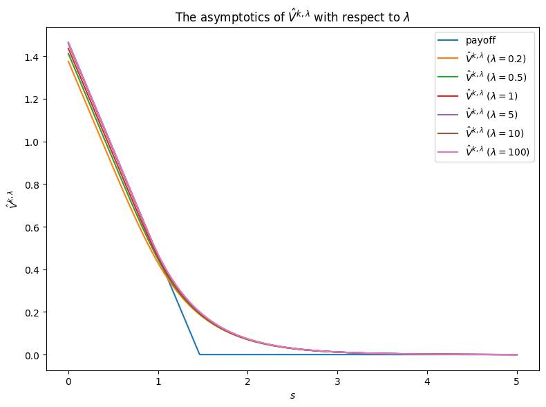
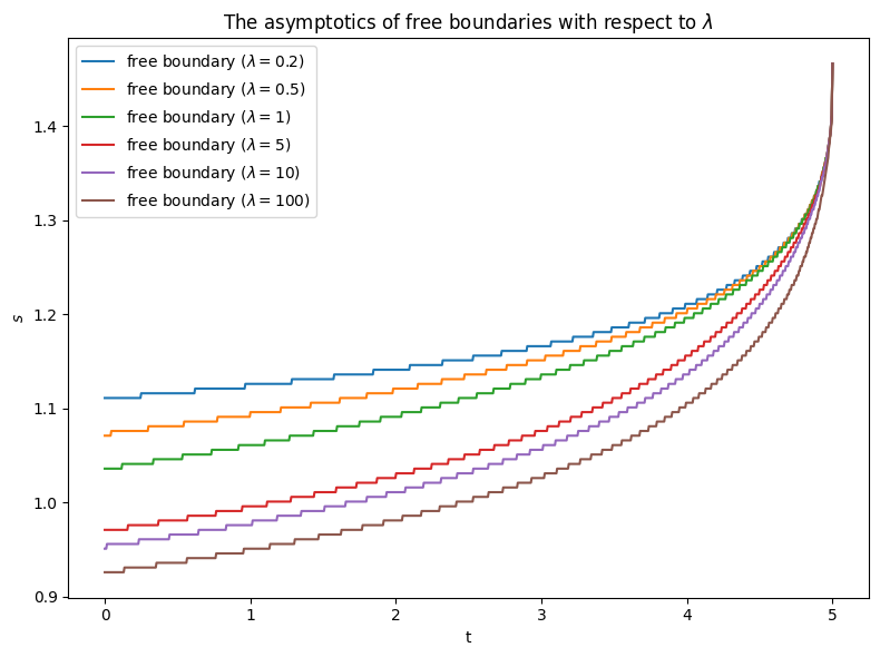
Figure 1: The asymptotic behaviours of the value functions and the free boundaries with respect to $\lambda$. Parameters: $\sigma=0.2,\underline{r}=0.02,\overline{r}=0.05,\eta=0.1,T=5,k=4.$

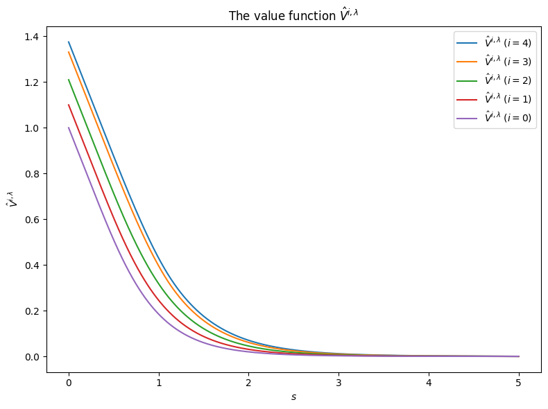
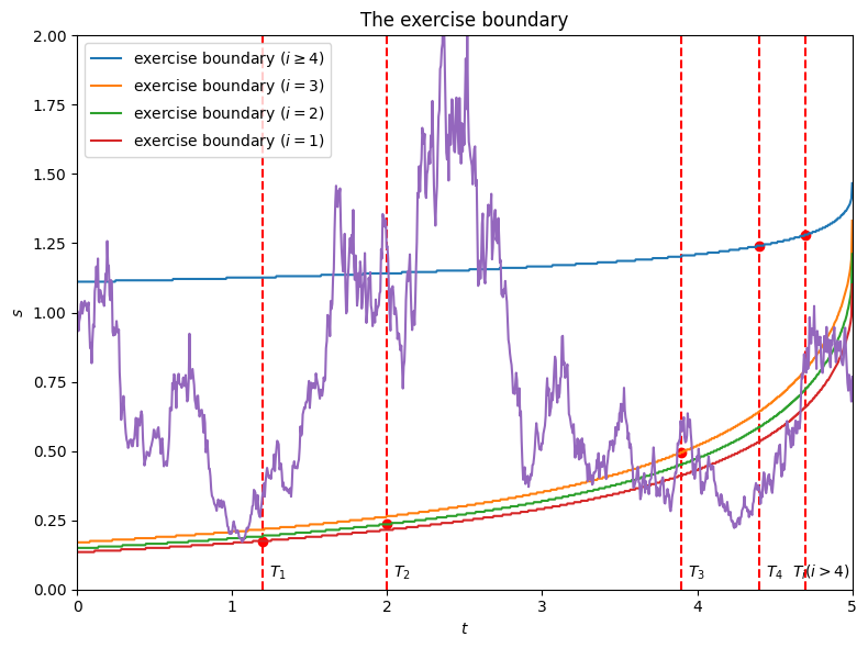
Figure 2: The value functions and the free boundaries at Poisson random times. Parameters: $\sigma=0.2,\underline{r}=0.02,\overline{r}=0.05,\eta=0.1,T=5,k=4,\lambda=0.2.$

References

• [1] Erhan Bayraktar and Song Yao. Optimal stopping for non-linear expectations–Part II. Stochastic Processes and their Applications, 121(2):212–264, 2011.
• [2] Katia Colaneri and Tiziano De Angelis. A class of recursive optimal stopping problems with applications to stock trading. Mathematics of Operations Research, 47(3):1833–1861, 2022.
• [3] Jaksa Cvitanic and Ioannis Karatzas. Backward stochastic differential equations with reflection and Dynkin games. The Annals of Probability, 24(4):2024–2056, 1996.
• [4] Roxana Dumitrescu and Marie-Claire Quenez and Agnès Sulem. A weak dynamic programming principle for combined optimal stopping/stochastic control with $\mathcal{E}^{f}$-expectations. SIAM Journal on Control and Optimization, 54(4):2090–2115, 2016.
• [5] Roxana Dumitrescu. An optional decomposition of $\mathcal{Y}^{g,\xi}-submartingales$ and applications to the hedging of American options in incomplete markets. arXiv:1901.02505, 2019.
• [6] Paul Dupuis and Hui Wang. Optimal stopping with random intervention times. Advances in Applied Probability, 34(1):141–157, 2002.
• [7] Nicole El Karoui, Christophe Kapoudjian, Étienne Pardoux, Shige Peng, and Marie-Claire Quenez. Reflected solutions of backward SDEs, and related obstacle problems for PDEs. The Annals of Probability, 25(2):702–737, 1997.
• [8] Miryana Grigorova, Peter Imkeller, Elias Offen, Youssef Ouknine, and Marie-Claire Quenez. Reflected BSDEs when the obstacle is not right-continuous and optimal stopping. The Annals of Applied Probability, 27(5):3153–3188, 2017.
• [9] Miryana Grigorova, Peter Imkeller, Youssef Ouknine, and Marie-Claire Quenez. Optimal stopping with f-expectations: the irregular case. Stochastic Processes and their Applications, 130(3):1258–1288, 2020.
• [10] Miryana Grigorova, Marie-Claire Quenez, and Agnès Sulem. American options in a non-linear incomplete market model with default. Stochastic Processes and their Applications, 142:479–512, 2021.
• [11] Saïd Hamadène, Jean-Pierre Lepeltier, and Zhen Wu. Infinite horizon reflected backward stochastic differential equations and applications in mixed control and game problems. Probability and Mathematical Statistics, 19(2):211–234, 1999.
• [12] Said Hamadène and Youssef Ouknine. Reflected backward stochastic differential equation with jumps and random obstacle. Electronic Journal of Probability, 8:1–20, 2003.
• [13] Said Hamadène and Youssef Ouknine. Reflected backward SDEs with general jumps. Theory of Probability & Its Applications, 60(2):263–280, 2016.
• [14] David Hobson and Matthew Zeng. Constrained optimal stopping, liquidity and effort. Stochastic Processes and their Applications, 150:819–843, 2022.
• [15] David Hobson. The shape of the value function under Poisson optimal stopping. Stochastic Processes and their Applications, 133:229–246, 2021.
• [16] Jean Jacod. Grossissement initial, hypothèse H’ et théorème de Girsanov. In Grossissements de filtrations: exemples et applications, pages 15–35. Springer, 1985.
• [17] Thierry Jeulin and Marc Yor. Grossissements de filtrations: exemples et applications: Séminaire de Calcul Stochastique 1982/83 Université Paris VI, volume 1118. Springer, 2006.
• [18] Ying Jiao, Idris Kharroubi, and Huyên Pham. Optimal investment under multiple defaults risk: a BSDE-decomposition approach. The Annals of Applied Probability, 23(2):455–491, 2013.
• [19] Idris Kharroubi and Thomas Lim. Progressive enlargement of filtrations and backward stochastic differential equations with jumps. Journal of Theoretical Probability, 27(3):683–724, 2014.
• [20] Edward Kim, Tianyang Nie, and Marek Rutkowski. American options in nonlinear markets. Electronic Journal of Probability, 26:1–41, 2021.
• [21] Jukka Lempa. Optimal stopping with information constraint. Applied Mathematics & Optimization, 66(2):147–173, 2012.
• [22] Jean-Pierre Lepeltier and Mingyu Xu. Penalization method for reflected backward stochastic differential equations with one r.c.l.l. barrier. Statistics and Probability Letters, 75(1):58–66, 2005.
• [23] Gechun Liang, Eva Lütkebohmert, and Wei Wei. Funding liquidity, debt tenor structure, and creditor’s belief: an exogenous dynamic debt run model. Mathematics and Financial Economics, 9(4):271–302, 2015.
• [24] Gechun Liang. Stochastic control representations for penalized backward stochastic differential equations. SIAM Journal on Control and Optimization, 53(3):1440–1463, 2015.
• [25] Gechun Liang and Haodong Sun. Dynkin games with Poisson random intervention times. SIAM Journal on Control and Optimization, 57(4):2962–2991, 2019.
• [26] José-Luis Menaldi and Maurice Robin. On some optimal stopping problems with constraint. SIAM Journal on Control and Optimization, 54(5):2650–2671, 2016.
• [27] José-Luis Menaldi and Maurice Robin. On some impulse control problems with constraint. SIAM Journal on Control and Optimization, 55(5):3204–3225, 2017.
• [28] José-Luis Menaldi and Maurice Robin. On some ergodic impulse control problems with constraint. SIAM Journal on Control and Optimization, 56(4):2690–2711, 2018.
• [29] Zbigniew Palmowski, Jose Luis Perez, Budhi Arta Surya, and Kazutoshi Yamazaki. The Leland-Toft optimal capital structure model under Poisson observations. Finance and Stochastics, 24:1035–1082, 2020.
• [30] Huyen Pham. Stochastic control under progressive enlargement of filtrations and applications to multiple defaults risk management. Stochastic Processes and their Applications, 120(9):1795–1820, 2010.
• [31] Marie-Claire Quenez and Agnès Sulem. BSDEs with jumps, optimization and applications to dynamic risk measures. Stochastic Processes and their Applications, 123(8):3328–3357, 2013.
• [32] Marie-Claire Quenez and Agnès Sulem. Reflected BSDEs and robust optimal stopping for dynamic risk measures with jumps. Stochastic Processes and their Applications, 124(9):3031–3054, 2014.
• [33] Christoph Reisinger and Yufei Zhang. Error estimates of penalty schemes for quasi-variational inequalities arising from impulse control problems. SIAM Journal on Control and Optimization, 58(1):243–276, 2020.
• [34] Zhen Wu. Fully coupled FBSDE with Brownian motion and Poisson process in stopping time duration. Journal of the Australian Mathematical Society, 74(2):249–266, 2003.
Refer to caption
Refer to caption