Observational Evidence for Magnetic Field Amplification in SN 1006
Abstract
We report the first observational evidence for magnetic field amplification in the north-east/south-west (NE/SW) shells of supernova remnant SN 1006, one of the most promising sites of cosmic ray (CR) acceleration. In previous studies, the strength of magnetic fields in these shells was estimated to be 25G from the spectral energy distribution, where the synchrotron emission from relativistic electrons accounted for radio to X-rays, along with the inverse Compton emission extending from the GeV to TeV energy bands. However, the analysis of broadband radio data, ranging from 1.37 GHz to 100 GHz, indicated that the radio spectrum steepened from to by = 0.85 0.21. This is naturally interpreted as a cooling break under strong magnetic field of 2 mG. Moreover, the high-resolution MeerKAT image indicated that the width of the radio NE/SW shells was broader than that of the X-ray shell by a factor of only 320, as measured by Chandra. Such narrow radio shells can be naturally explained if the magnetic field responsible for the radio emissions is 2 mG. Assuming that the magnetic field is locally enhanced by a factor of approximately = 100 along the NE/SW shells, we argue that the filling factor, which is the volume ratio of such a magnetically enhanced region to that of the entire shell, must be as low as approximately = 2.510-5.
1 Introduction
Young supernova remnants (SNRs) are considered to be promising sites for the production of galactic cosmic ray (CRs) through diffusive shock acceleration (DSA; Bell, 1978; Blandford & Eichler, 1987; Malkov & Drury, 2001), although the detailed process of DSA is not well understood. In particular, the magnetic field strength and structure are vital for determining the maximum energy of particles that can be accelerated in the shock.
SN 1006, located at a distance of 1.8 kpc (Green, 2001), is a prototypical example wherein synchrotron X-ray emissions along the outer north-east (NE) and south-west (SW) shells are detected through observation from the ASCA. Assuming an estimated magnetic field of 6–10 G, Koyama et al. (1995) found that electrons of 100 TeV were being accelerated in the shock of SN 1006. High-resolution Chandra Advanced CCD Imaging Spectrometer (ACIS) images revealed that the X-ray shells were extremely thin with scale widths of 4″(0.04 pc) and 20″(0.2 pc) in the upstream and downstream regions, respectively (Bamba et al., 2003). The authors assumed downstream and upstream magnetic field strengths of = 4 = 40 G, although larger values, namely, 150 G, are suggested with field amplification (Ksenofontov et al., 2005).
Very high energy gamma rays (above 100 GeV) from SN 1006 were detected by the High Energy Stereoscopic System (H.E.S.S.) (Acero et al. (2010)). Together with the GeV gamma-ray observation from the Fermi-Large Area Telescope (LAT) over 10 years observations, Xing et al. (2019) suggested that the spectral energy distribution (SED) was well represented by a one-zone leptonic model, wherein synchrotron emission constituted the low energy bump from radio to X-rays, whereas inverse Compton (IC) emission on cosmic microwave background (CMB) accounts for the high energy bump in GeV/TeV gamma rays. Based on SED modeling, the magnetic field strengths were estimated to be 24 G and 30 G for the NE and SW shells, respectively. However, recent Planck observations indicated a spectral curvature above 10 GHz (Arnaud et al. (2016)); thus, the radio-to-X-ray spectrum may not connect smoothly as opposed to that determined by SED models by various authors. This is supported by the fact that the optical/ultra-violet (UV) counterpart of SN 1006 is extremely faint except for the bright H filament in the NW shell (Winkler et al., 2003; Korreck et al., 2004).
Comparisons with similar young SNRs may provide some hints to solve the contradiction regarding the magnetic field strengths. For example, the overall SED of RX J1713.73946 is well represented by the synchrotron and IC (CMB) model with 10 G, as in the case of SN 1006 (but see Ellison et al. (2010) to account for the overall spectrum of RX J1713.73946 with a hadronic model). However, short time variability on a one-year timescale was found in the shell of RX J1713.73946; thus, the magnetic field in the hot spot should be as high as 1 mG (Uchiyama et al. (2007)). Similar to that of RX J1713.73946, Cassiopia A indicates very thin non-thermal X-ray fillament along the shock, and a fast variability timescale of 4 years was found, which also suggests the amplification of the magnetic field to 1 mG (Uchiyama & Aharonian (2008)).
In this Letter, we present new and independent evidence for magnetic field amplification in the NE/SW shells of SN 1006. In particular, we did not rely on detecting such short time variability but focused on the spectral and imaging results. We presented the systematic analysis of radio data from 1.4 to 100 GHz to confirm the spectral break in the radio spectrum. We also estimated the optical and UV fluxes to fill in the SED gap between radio and X-rays. Finally, we compared the high-resolution radio and X-ray image, which provides independent evidence for an enhanced magnetic field in the NE/SW shell of SN 1006, and then subsequently presented the conclusion of our findings.
2 Analysis and result
2.1 Broadband Radio Spectrum
We analyzed all the archival Planck-low frequency instrument (LFI) data containing 30, 44, and 70 GHz fluxes, and 100 GHz data from high frequency instrument (HFI) to identify the high frequency spectral features of SN 1006. Based on Arnaud et al. (2016), the flux densities were measured using standard aperture photometry, with the source size centered on SN 1006 and the diameter scaled to = 1.5 . Here, is the source size estimated from = , where and are the spatial distribution of SN 1006 and the Planck beam size (Ade et al., 2014a; Aghanim et al., 2014a), respectively. is 15′ and are 16.2′ at 30 GHz, 13.6′ at 44 GHz and 6.7′ at 70GHz, and 4.83′ at 100 GHz. We also estimated and subtracted the background from the area between concentric circles with inner and outer radii of 1.5 and 2.0 , respectively. An aperture correction was applied to correct for the loss of flux density outside the aperture. The uncertainties for the flux densities were the root-sum-square of calibration uncertainty (Ade et al., 2014b; Aghanim et al., 2014b) and propagated statistical errors. The statistical errors considered the number of pixels in the source aperture and background annulus, and the standard deviation within the background annulus (Arnaud et al., 2016).
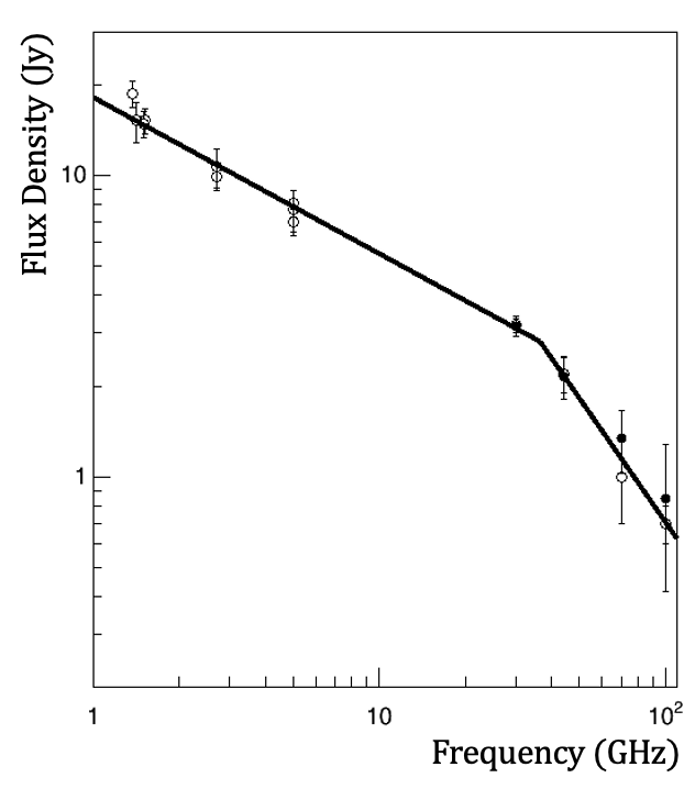
Figure 1 shows the broadband radio spectrum of SN 1006 as measured with Planck ( ), along with a collection of previous measurements ranging from 1.4 to 100 GHz ( ). The spectrum cannot be represented by a single power law of , where is the flux density at frequency . Rather, it can be well represented by a broken power law with a break frequency of , above which the spectral index steepens from to , where the reduced chi-squared for the fitting is /dof = 6.74/13. The confidence level that the broken power law is a better representation of the data than a single power law is 99.9 (3.59 ) based on the -test.
2.2 Estimation of the Optical and UV Fluxes
The optical emission of SN 1006 is extremely faint except for the bright H filament as observed in the NW shell (Winkler et al., 2003). Thus, the only H filament has been extensively studied in terms of proper motion, as well as comparison with the shock structure in optical and X-rays. Compared with the maximum surface brightness for the filament, namely, , the intensity of the diffuse emission associated with NE/SW shells of SN 1006 is fainter tham a factor of 2025 (see Fig.3 of Winkler et al. 2003). Assuming a region size of 70 arcmin2 for the NE shell, the integrated flux would be . Considering the entire SN 1006, we simply doubled the NE flux assuming that a similar amount of flux would by contributed by the SW shell.
The UV flux in SN 1006 is also faint, as measured by the Far Ultraviolet Spectroscopic Explorer (FUSE). The flux density in the NE shell in the UV range is approximately between 1010 and 1050 Å (see Fig.2 of Korreck et al. 2004). Considering the relatively narrow field of view (30″ 30″) of FUSE, the integrated NE flux is estimated to be for the assumed region size of 70 arcmin2. We simply doubled the NE flux to estimate the flux from entire region of SN 1006.
2.3 Direct comparison of radio/X-ray shells
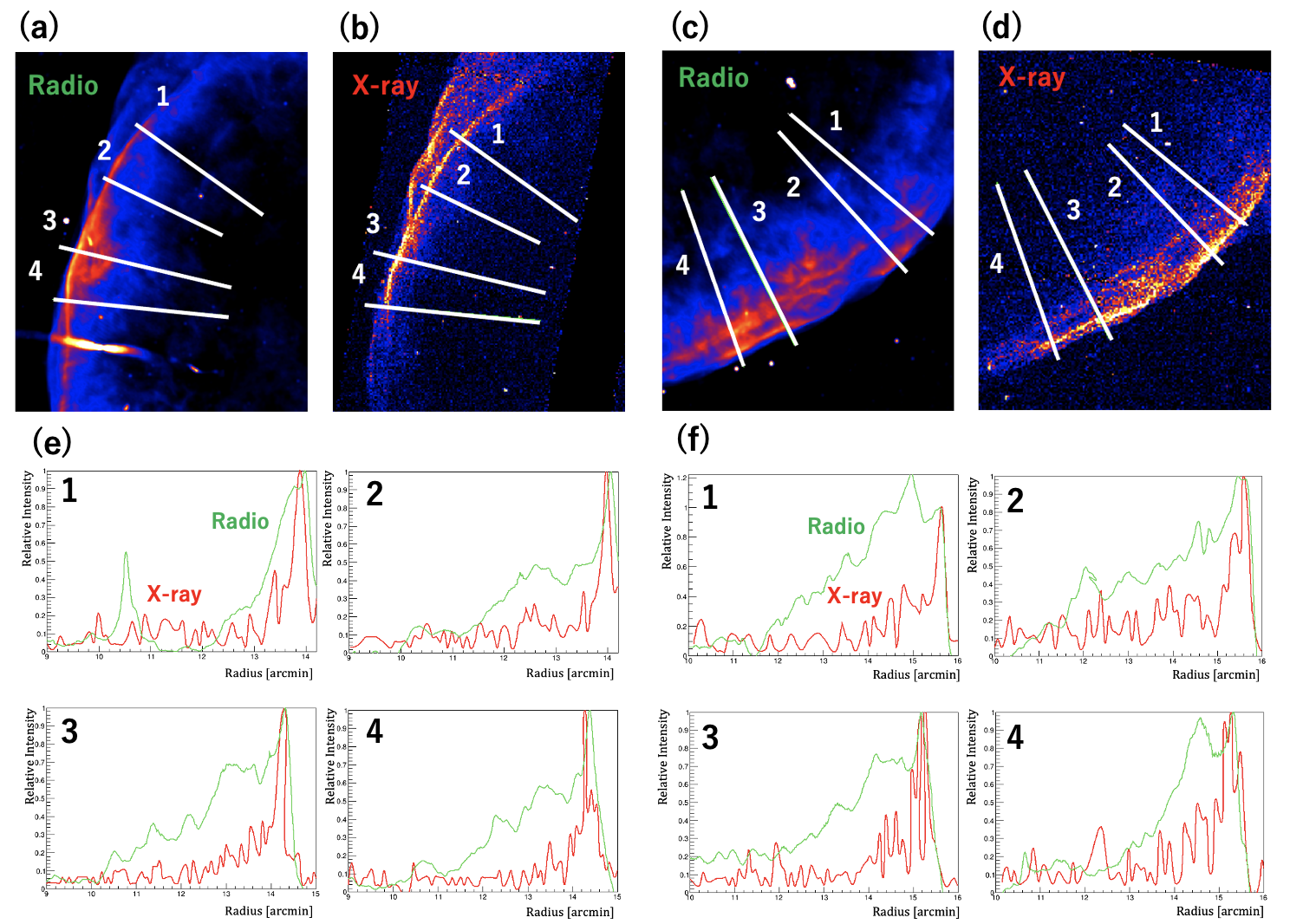
Although SN 1006 is a prototypical SNR that clearly exhibits non-thermal shells/filaments in both radio and X-rays, direct comparisons have not been made until now using high resolution radio and X-ray images with angular resolutions better than scale width ( 10″) of the intrinsic shell width. Figure 2 shows the radial profiles of NE/SW shells of SN 1006, as compared with those of the radio (1335 MHz; MeerKAT) and X-rays (2.07.0 keV ; Chandra). Comparisons were made across various parts of the shells along the lines. MeerKAT is a radio telescope in Northern Cape province of South Africa (Jonas, 2009), whose angular resolution at 1335 MHz is 8″(Cotton et al., 2024). This is still worse than the X-ray image resolution provided by Chandra ACIS ( 05) but better than that of the previous image provided by the Very Large Array (e.g., 20″; Reynolds & Gilmore 1986). Figure 2 clearly shows that the radio shell is broader than that of X-rays, but at most, it is only approximately 10-fold of both the NE and SW shells.
3 Discussion and Conclusion
3.1 Estimation of the magnetic field strength
In 2.1, we reported that the broadband radio spectrum showed a spectral break at = 36 6 GHz, at which the spectrum steepened from to by = 0.85 0.21. This result has confirmed the finding of Arnaud et al. (2016). Notably, that such a break in the spectral index is often seen as a result of synchrotron losses in various active galactic nuclei (AGNs) (e.g., Inoue & Takahara, 1996; Kataoka et al., 1999). Assuming that this is a cooling break at which the electron-cooling time and dynamical timescale of SNR are balanced, we expect at = . For the synchrotron emission, the cooling time of electrons can be expressed as , where is the Lorentz factor of electrons emitting photons in the magnetic field , and (e.g., Rybicki & Lightman, 1985). Subsequently, we can obtain
| (1) |
The dynamical timescale of SNR, , can be regarded as the advection time of electrons across the shock, which should be shorter than the age of the SNR. Substituting the age of SN 1006, namely, 1 kyr, for , we can obtain a lower limit of 2 mG for = 36 GHz. This is the magnetic field estimated from the “cooling break” in the radio spectrum. In this formulation, only the synchrotron cooling is considered. The contribution from the cooling of IC (CMB) cooling is more than one order of magnitude smaller and can be ignored as we descibed below.
Another way of estimating the magnetic field from the observed radio flux is to assume an equipartition (i.e., minimum energy) between the electron and magnetic field energy densities, = . This can be expressed as
| (2) |
where and are the distance and volume of the SNR, and is the flux density at frequency (eg. Longair (1994)). is the ratio of the energy stored in electrons and protons, where = 1 for - plasma. Consequently, we obtained 5 G. Instead, if we assume a typical CR composition, 100, 10 G is obtained. Hence, the magnetic field estimated from the equipartition is an order of 10G regardless of the plasma content; thus, .
3.2 Implication from SED
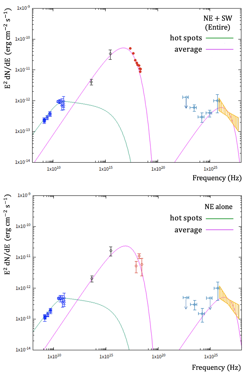
Subsequently, we construct the SED from radio to TeV gamma rays, including the broadband radio spectrum and optical/UV fluxes newly derived in this study. Figure 3 shows the broadband SED of the entire SN 1006 (NE + SW shells) and that of the NE shell alone. In previous studies, the overall SED was modeled by one-zone synchrotron/IC(CMB) emissions with s moderate magnetic field of G (e.g., Xing et al., 2019). However, according to our results, multiple components are necessary to account for the radio-to-X-ray spectrum. Notably, the first synchrotron component dominates the radio emissions but flattens above . The second synchrotron component appears weak in the radio band but accounts for most of the optical-UV-X-ray emission without turnover.
Thus, we assumed “double” electron populations to reproduce the overall structure of the SED; the first population is responsible for the synchrotron emission in compact regions or hot spots where the magnetic field is enhanced by a factor of 100; thus, . Conversely, the second population radiates another synchrotron emission in the “average” magnetic field of . Although the geometry of the magnetic enhanced regions is still unknown, the similarity of the radio and X-ray images, as shown in Figure 2, may imply that such regions are almost uniformly distributed along the shock as either compact patches, like hot spots, or as diffuse sheets/filaments. Hereafter, we call such magnetically enhanced regions “hot spots” for simplicity. In any case, we can constrain the filling factor , which is the volume ratio of such magnetically enhanced regions to the entire shell, from the observed SED. The radio flux in the hot spots is expressed as . Assuming that the radio emissions of hot spots is 10–100 times brighter than that of the other (i.e., average) parts of the SNR, (1)V, we obtain 10–100; thus, 10-5 10-4.
An example of SED fits is also shown in Figure 3 assuming a filling factor of = 2.510-5. The represents the synchrotron/IC (CMB) emission from entire (average) region, whereas the curve is the synchrotron emission in the hot spots. Notably, the corresponding IC (CMB) emission in the hot spot is too low to appear in this figure. The first electron population has a cooling break at = 2103 (or = 1 GeV), above which the electron spectral index steepened from 2.1 to 3.1. We assumed that = 2.5 mG in the hot spots to be consistent with the observed break at = 36 GHz. In contrast, the second population has no break in the electron spectrum with = 2.0 up to the maximum frequency of = 1.0 (or = 51 TeV). The magnetic fields were assumed to be = 25 G and 18 G for the entire SN 1006 and NE shell, respectively. Table 1 summarizes the fitting parameters of the SEDs. Note that is well determined within an uncertainty of 30 , whereas = 2.5 mG, is just an example of possible fitting parameters. Similarly, = 1.0 106 for the hot spots is an assumption because it cannot be determined solely from the SED.
| Parameter | Entire (hot spots) | Entire (average) |
|---|---|---|
| 1 | 1 | |
| index | 2.1 | 2.0 |
| [G] | ||
| volume [pc3] | ||
| parameter | NE (hot spots) | NE (average) |
| 1 | 1 | |
| index | 2.1 | 2.0 |
| [G] | ||
| volume [pc3] |
Notes: As for an electron population in the hot spots, we assumed a broken power law function with an exponential cut-off, for , whereas for . For remaining average region, we assumed a simple power law function with an exponential cutoff, .
3.3 Comparison between Radio/X-ray of the NE/SW shells
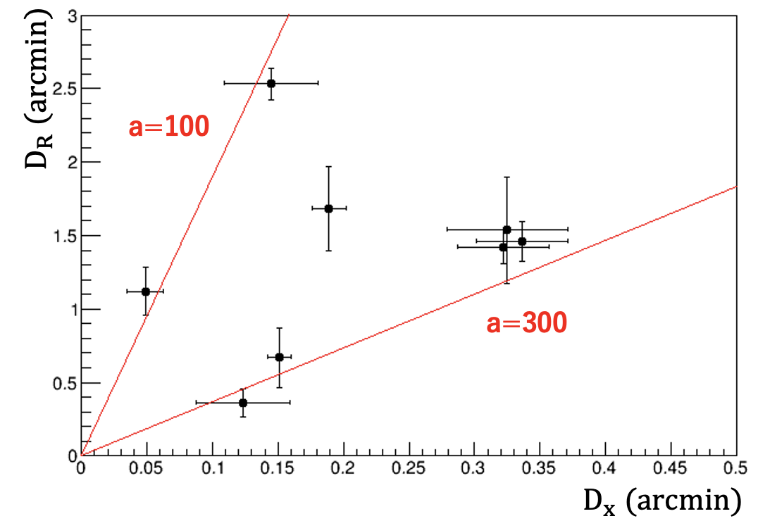
Subsequently, we discuss the spatial extent of the NE/SW shells as observed with the radio and X-ray images shown in Figure 2. In general, the thickness of the shell can roughly be estimated as , where is the shock speed and is the cooling time of electrons that emit photons of certain energies. Therefore, if the magnetic field for radio and X-ray emissions are the same, the thickness of the shell measured in radio () and X-rays () reflects the difference of ; thus, . Hence, we expect 2104, which is, however, far from what is shown in Figure 2. In fact, the width of NE/SW shells, defined here as the full width at half maximum (FWHM) of the peak differs by a factor of 320, as shown in Figure 4. Moreover, this difference is not owing to the different angular resolutions between Chandra and MeerKAT, as the width of the NE/SW shells is generally broader than 04 in the radio band, that is more than three times that of the MeerKAT angular resolution.
The observed also indicates that the magnetic fields, which mainly contribute to the observed radio and X-ray emissions, cannot be the same. In such a case,
| (3) |
where and are the magnetic fields responsible for the radio and X-ray emissions. The observed ratio of , can be converted to the amplification factor of the magnetic field as . This is consistent with magnetic field amplification in the hot spots, namely, 100, which is independently estimated from the SED.
Finally, assuming = 2.5 mG and = 25 G, the thickness of the shell is estimated as approximately 3.7 pc (or 72) and 0.2 pc (or 04) for 103 km/s. This is slightly larger, but almost consistent with that observed in the NE/SW shells as shown in Figures 2 and 4.
3.4 Comparison with other SNRs
The manifestation of hot spots with a strong magnetic field of of approximately 1 mG has been reported in similar young SNRs such as RX J1713.73946 (Uchiyama et al., 2007) and Cassiopeia A (Uchiyama & Aharonian, 2008). In both objects, the flickering of X-ray hot spots on yearly scales was observed. Meanwhile, the overall SED of RX J1713.73946 is well represented by the synchrotron/IC (CMB) model with of 10 G (Abdo et al., 2011), although even larger of 250 G is suggested for the case of Cassiopeia A (Saha et al., 2014). The filling factor of such hot spots, namely, , is not discussed in Uchiyama et al. (2007), but they have suggested that the X-ray emissions from the hot spots is less than approximately 1/100 of the entire emission of the SNR, which is consistent with the present observation of SN 1006 (see Figure 3). Note, however, that the anticipated linear size of the hot spots in SN 1006 would be approximately 2.910-2 times smaller than the typical shell thickness of approximately 10″. Thus this is difficult to resolve, even with Chandra.
The physical mechanism of magnetic amplification in the hot spots remains quite uncertain in all the SNRs. In the standard theory of shock compression, = / = / = 4, where and are the downstream and upstream magnetic fields and and are the downstream and upstream energy densities of the plasma, respectively. Thus 100 is hardly explained by the classical shock theory. Instead, such a strong magnetic field may be produced owing to the turbulent dynamo action through shock-cloud interactions as suggested for RX J1713.73946 (Inoue et al., 2011); however, this cannot be the case for a relatively “clean” environment as in SN 1006 and Cassiopeia A (but see, Miceli et al. 2014). In this context, some particle-in-cell (PIC) simulations of non-relativistic perpendicular shocks in the high-Mach-number () suggests magnetic amplification of = 5.5(); thus 100 for 400 or 4000 km s-1 (Bohdan et al. (2021)). However, whether similar efficient amplification is possible even in parallel shocks is uncertain as observed in SN 1006 (Reynoso et al., 2013; Zhou et al., 2023). Similar analysis using Planck, MeerKAT, and Chandra is ongoing for other types of SNRs to systematically understand the physical origin of magnetic amplification.
References
- Abdo et al. (2011) Abdo, A., Ackermann, M., Ajello, M., et al. 2011, The Astrophysical Journal, 734, 28
- Acero et al. (2010) Acero, F., Aharonian, F., Akhperjanian, A., et al. 2010, Astronomy & Astrophysics, 516, A62
- Ade et al. (2014a) Ade, P., Aghanim, N., Armitage-Caplan, C., et al. 2014a, Astronomy & Astrophysics, 571, A7
- Ade et al. (2014b) —. 2014b, Astronomy & Astrophysics, 571, A8
- Aghanim et al. (2014a) Aghanim, N., Armitage-Caplan, C., Arnaud, M., et al. 2014a, Astronomy & Astrophysics, 571, A4
- Aghanim et al. (2014b) —. 2014b, Astronomy & Astrophysics, 571, A5
- Arnaud et al. (2016) Arnaud, M., Ashdown, M., Atrio-Barandela, F., et al. 2016, Astronomy & Astrophysics, 586, A134
- Bamba et al. (2003) Bamba, A., Yamazaki, R., Ueno, M., & Koyama, K. 2003, The Astrophysical Journal, 589, 827
- Bamba et al. (2008) Bamba, A., Fukazawa, Y., Hiraga, J. S., et al. 2008, Publications of the Astronomical Society of Japan, 60, S153
- Bell (1978) Bell, A. 1978, Monthly Notices of the Royal Astronomical Society, 182, 147
- Blandford & Eichler (1987) Blandford, R., & Eichler, D. 1987, Physics Reports, 154, 1
- Bohdan et al. (2021) Bohdan, A., Pohl, M., Niemiec, J., et al. 2021, Physical review letters, 126, 095101
- Cotton et al. (2024) Cotton, W., Kothes, R., Camilo, F., et al. 2024, The Astrophysical Journal Supplement Series, 270, 21
- Dyer et al. (2009) Dyer, K., Cornwell, T., & Maddalena, R. 2009, The Astronomical Journal, 137, 2956
- Ellison et al. (2010) Ellison, D. C., Patnaude, D. J., Slane, P., & Raymond, J. 2010, The Astrophysical Journal, 712, 287
- Gardner & Milne (1965) Gardner, F., & Milne, D. 1965, The Astronomical Journal, 70, 754
- Green (2001) Green, D. A. 2001, Cambridge: Mullard Radio Astron: Obs
- Inoue & Takahara (1996) Inoue, S., & Takahara, F. 1996, Astrophysical Journal v. 463, p. 555, 463, 555
- Inoue et al. (2011) Inoue, T., Yamazaki, R., Inutsuka, S.-i., & Fukui, Y. 2011, The Astrophysical Journal, 744, 71
- Jonas (2009) Jonas, J. L. 2009, Proceedings of the IEEE, 97, 1522
- Kalemci et al. (2006) Kalemci, E., Reynolds, S. P., Boggs, S. E., et al. 2006, The Astrophysical Journal, 644, 274
- Kataoka et al. (1999) Kataoka, J., Mattox, J., Quinn, J., et al. 1999, The Astrophysical Journal, 514, 138
- Korreck et al. (2004) Korreck, K., Raymond, J., Zurbuchen, T., & Ghavamian, P. 2004, The Astrophysical Journal, 615, 280
- Koyama et al. (1995) Koyama, K., Petre, R., Gotthelf, E., et al. 1995, Nature, 378, 255
- Ksenofontov et al. (2005) Ksenofontov, L. T., Berezhko, E., & Völk, H. 2005, Astronomy & Astrophysics, 443, 973
- Kundu (1970) Kundu, M. 1970, Astrophysical Journal, vol. 162, p. 17, 162, 17
- Longair (1994) Longair, M. S. 1994, High Energy Astrophysics (Cambridge University Press), doi: 10.1017/CBO9781139170505
- Malkov & Drury (2001) Malkov, M., & Drury, L. O. 2001, Reports on Progress in Physics, 64, 429
- Miceli et al. (2014) Miceli, M., Acero, F., Dubner, G., et al. 2014, The Astrophysical Journal Letters, 782, L33
- Milne (1971) Milne, D. 1971, Australian Journal of Physics, vol. 24, p. 757, 24, 757
- Milne & Dickel (1975) Milne, D., & Dickel, J. 1975, Australian Journal of Physics, 28, 209
- Petruk et al. (2009) Petruk, O., Dubner, G., Castelletti, G., et al. 2009, Monthly Notices of the Royal Astronomical Society, 393, 1034
- Reynolds & Gilmore (1986) Reynolds, S. P., & Gilmore, D. M. 1986, Astronomical Journal (ISSN 0004-6256), vol. 92, Nov. 1986, p. 1138-1144., 92, 1138
- Reynoso et al. (2013) Reynoso, E. M., Hughes, J. P., & Moffett, D. A. 2013, The Astronomical Journal, 145, 104
- Rothenflug et al. (2004) Rothenflug, R., Ballet, J., Dubner, G., et al. 2004, Astronomy & Astrophysics, 425, 121
- Rybicki & Lightman (1985) Rybicki, G. B., & Lightman, A. P. 1985, Radiative Processes in Astrophysics (New York, NY: Wiley), doi: 10.1002/9783527618170
- Saha et al. (2014) Saha, L., Ergin, T., Majumdar, P., Bozkurt, M., & Ercan, E. 2014, Astronomy & Astrophysics, 563, A88
- Uchiyama & Aharonian (2008) Uchiyama, Y., & Aharonian, F. A. 2008, The Astrophysical Journal, 677, L105
- Uchiyama et al. (2007) Uchiyama, Y., Aharonian, F. A., Tanaka, T., Takahashi, T., & Maeda, Y. 2007, Nature, 449, 576
- Winkler et al. (2003) Winkler, P. F., Gupta, G., & Long, K. S. 2003, The Astrophysical Journal, 585, 324
- Xing et al. (2019) Xing, Y., Wang, Z., Zhang, X., & Chen, Y. 2019, Publications of the Astronomical Society of Japan, 71, 77
- Zhou et al. (2023) Zhou, P., Prokhorov, D., Ferrazzoli, R., et al. 2023, The Astrophysical Journal, 957, 55