A minimal model for multigroup adaptive SIS epidemics

Abstract

We propose a generalization of the adaptive N-Intertwined Mean-Field Approximation (aNIMFA) model studied in Achterberg and Sensi [1] to a heterogeneous network of communities. In particular, the multigroup aNIMFA model describes the impact of both local and global disease awareness on the spread of a disease in a network. We obtain results on existence and stability of the equilibria of the system, in terms of the basic reproduction number $R_{0}$. Under light constraints, we show that the basic reproduction number $R_{0}$ is equivalent to the basic reproduction number of the NIMFA model on static networks. Based on numerical simulations, we demonstrate that with just two communities periodic behaviour can occur, which contrasts the case with only a single community, in which periodicity was ruled out analytically. We also find that breaking connections between communities is more fruitful compared to breaking connections within communities to reduce the disease outbreak on dense networks, but both strategies are viable to networks with fewer links. Finally, we emphasise that our method of modelling adaptivity is not limited to SIS models, but has huge potential to be applied in other compartmental models in epidemiology.

1 Introduction

Various approaches have been suggested to model the response of individuals to an epidemic. A common approach is to apply an SIR-like (Susceptible – Infected – Recovered) compartmental model by including an Aware compartment [2, 3, 4, 5, 6]. Aware individuals are conscious of the ongoing disease and are therefore more cautious towards contact with other individuals. Thus, aware individuals are less likely to be infected. Moreover, some authors included the possibility of corruption of information spreading throughout a population [7, 8, 9], which has been very problematic throughout the COVID-19 pandemic in particular [10].

Other authors suggested local rules to model personal risk mitigation using link rewiring schemes [11] or link-breaking rules [12, 13]. These models primarily consider personal decisions of nodes to apply mitigation strategies, who generally base their decision on the presence of the disease in the local neighbourhood around that node. On the contrary, the overall presence of the disease in the population is often neglected. A recent paper, conversely, proposed an interesting game-theoretical approach to the coupling of infectious disease spreading and global awareness [14].

In reality, both personal risk perception and global knowledge of the disease persistence in the population play a role in the mitigation strategy. Here, we propose a multigroup adaptive SIS (Susceptible – Infected – Susceptible) model, based on the simple model for adaptive SIS epidemics [1]. The multigroup approach is convenient to describe heterogeneity amongst agents using a system of ODEs, by considering the evolution of a disease in a network of communities [15, 16, 17, 18, 19, 20, 21, 22, 23]. The disease evolves both within each community, in which homogeneous mixing is assumed, and between communities, depending on the strength of the links between those communities. The size of a community may vary between households to entire countries. Besides the usual split-up of the population in geographically separated groups, the communities mentioned above could also represent age-groups in the population and they are widely used for applications with real data to simulate the incidence of a disease stratified by age groups [24, 25, 26].

Even though the disease dynamics of the aNIMFA model is extremely simplified (only an SIS model is utilised), we expect the dynamics to be very rich and should be able to accurately capture many aspects of group-level risk mitigation during epidemic outbreaks. In particular, we show that periodic solutions may occur in an asymmetric network with just two communities, which contrasts the case with a single community, in which it was proven that limit cycles cannot occur [1].

The paper is structured as follows. In Section 2, we introduce our multigroup generalization of the aNIMFA model. In Section 3, we compute the basic reproduction number and prove the existence and stability of the disease-free equilibrium. Then, we prove the existence of at least one endemic equilibrium when the basic reproduction number is (slightly) larger than one. Section 4 showcases various numerical case studies of the aNIMFA model, including the emergence of periodic behaviour in just two communities. We conclude with Section 5.

2 The multigroup aNIMFA model

Achterberg and Sensi [1] introduced a simple model for adaptive SIS epidemics in a well-mixed population. The model is given by

$$\frac{\textnormal{d}y}{\textnormal{d}t} =-\delta y+\beta y(1-y)z,$$ (1a)

$$\frac{\textnormal{d}z}{\textnormal{d}t} =-\zeta zf_{\textnormal{br}}(y)+\xi(1-z)f_{\textnormal{cr}}(y),$$ (1b)

$$\qquad\qquad\text{feasible region }0\leq y\leq 1,0\leq z\leq 1$$

where $y,z$ represent the fraction of infected nodes (known as the prevalence) and the fraction of existing connections in the population, respectively. The fraction of infected nodes in (1a) decreases based on recovery (first term with rate $\delta$) and increases based on infections (second term with rate $\beta$). The link density in (1b) decreases (first term) based on the link-breaking process $f_{\textnormal{br}}$ with rate $\zeta$ and increases (second term) with the link-creation process $f_{\textnormal{cr}}(y)$ with rate $\xi$. The functional responses $f_{\textnormal{br}}$ and $f_{\textnormal{cr}}$ capture human behaviour and describe the people’s response to the ongoing epidemic. In particular, the functional responses $f_{\textnormal{br}}$ and $f_{\textnormal{cr}}$ depend directly on the prevalence $y$. It is assumed that $f_{\textnormal{br}}$ and $f_{\textnormal{cr}}$ are non-negative functions, i.e. $f_{\textnormal{br}}(y),f_{\textnormal{cr}}(y)\geq 0$ for all $0\leq y\leq 1$.

Here, we propose a generalisation of (1) to $n$ heterogeneous groups:

$$\frac{\textnormal{d}y_{i}}{\textnormal{d}t} =-\delta_{i}y_{i}+(1-y_{i})\sum_{j=1}^{n}\beta_{ij}y_{j}z_{ij},$$ (2a)

$$\frac{\textnormal{d}z_{ij}}{\textnormal{d}t} =-\zeta_{ij}z_{ij}f_{\textnormal{br,ij}}(y_{i},y_{j},\bar{y})+\xi_{ij}(1-z_{ij})f_{\textnormal{cr,ij}}(y_{i},y_{j},\bar{y}),$$ (2b)

$$\bar{y} =\frac{1}{n}\sum_{j=1}^{n}y_{j},$$ (2c)

$$\qquad\qquad\text{feasible region }0\leq y_{i}\leq 1,0\leq z_{ij}\leq 1\text{ for }1\leq i,j\leq n$$

where $y_{i}$ is the local prevalence in group $i$, $z_{ij}$ is the link density between group $i$ and $j$, $\delta_{i}$ is the curing rate of group $i$, $\beta_{ij}$ is the infection rate from group $j$ to group $i$, $\zeta_{ij}$ is the link-breaking rate between group $i$ and $j$, $\xi_{ij}$ is the link-creation rate between group $i$ and $j$ and $\bar{y}$ is the global prevalence (or simply the prevalence) of the infectious disease in the whole population, i.e. is the average prevalence over all communities. We are implicitly assuming here that all communities have the same size. In general, the functional responses $f_{\textnormal{br,ij}}$ and $f_{\textnormal{cr,ij}}$ can be different between each region $i$ and $j$. In particular, when $i=j$, the functional responses $f_{\textnormal{br,ii}}$ and $f_{\textnormal{cr,ii}}$ describe the different responses of each community $i$ to the internal spread of the infectious disease.

The $n$ communities can be represented as $n$ nodes in a graph $G$, where each node represents one community. The links in the graph $G$ constitute the connections $z_{ij}$ between community $i$ and $j$. We assume the graph $G$ is connected (i.e. the adjacency matrix $B=(\beta_{ij})$ is irreducible). From a biological point of view, a natural assumption would be to consider all $\delta_{i}$ equal, since they represent the inverse of the recovery rate of the same disease. However, each region may have a different healthcare quality, leading to potentially slightly different recovery rates $\delta_{i}$. Therefore, we keep the model (2) as general as possible.

Equation (2) is coined the multigroup adaptive N-Intertwined Mean-Field Approximation (multigroup aNIMFA), named after the NIMFA model [27]. On a technical note, Eq. (2) contains $n^{2}+n$ equations, not $n$, but we will adhere to the definition (2) due its analogy to the static NIMFA model [27]. We assume the parameters $\delta_{i}$, $\beta_{ij}$, $\zeta_{ij}$, $\xi_{ij}$ can be different for each node and link, and are assumed to be positive. The standard NIMFA model with link weights $z_{ij}=z_{ij}(0)$ is recovered if $\zeta_{ij}=\xi_{ij}=0$ for all $i$ and $j$. Furthermore, $f_{\textnormal{br,ij}}$ and $f_{\textnormal{cr,ij}}$ are assumed to be non-negative for all $0\leq y\leq 1$ and all $i$ and $j$. We emphasise here that the link density in the aNIMFA model is not necessarily symmetric, i.e. $z_{ij}\neq z_{ji}$. This allows us to capture unilateral decisions to limit or encourage movement between community $i$ and community $j$, but not vice versa. For example, we can think of some country A which lifts restrictions on incoming flights from another country B, even though country B still discourages its inhabitants to travel.

In an epidemic context, it is reasonable to assume that the breaking (respectively, creation) of contacts is non-decreasing (non-increasing) with respect to the current prevalence. Indeed, during epidemic peaks, people are more likely to isolate, and during periods of low prevalence, people are likely to enhance their social activities. Mathematically, this translates in the functions $f_{\textnormal{br,ij}}$ and $f_{\textnormal{cr,ij}}$ being non-decreasing and non-increasing in all their arguments, respectively. For the remainder of this work, we focus on the epidemic case and therefore assume non-decreasing $f_{\textnormal{br,ij}}$ and non-increasing $f_{\textnormal{cr,ij}}$.

Equations (2) describe the interplay between local and global awareness, where the functional response of the individuals to the disease is based on the local prevalences $y_{i}$ and $y_{j}$, and global prevalence $\bar{y}$, respectively. Similarly, the aNIMFA model distinguishes between the within-link-density $z_{ii}$ and cross-link-density $z_{ij}$, which allows for different or targeted counter-measures in specific communities.

Prior to investigating specific case studies, we first prove several results for the general case of system (2).

3 Analytical results

In this section, we provide numerous analytical results concerning system (2).

3.1 Boundedness of the feasible region

In the following Lemma, we prove that system (2) evolves in the biologically relevant region $[0,1]^{n+n^{2}}$.

Lemma 1.

Consider a solution of system (2) starting at $y_{i}(0)\in[0,1]$ and $z_{ij}(0)\in[0,1]$ for all $i$ and $j$. Recall that $f_{\textnormal{br,ij}}(y_{i},y_{j},\bar{y}),f_{\textnormal{cr,ij}}(y_{i},y_{j},\bar{y})\geq 0$ for all $y_{i},y_{j},\bar{y}\in[0,1]$ and all $i,j$. Then, $y_{i}(t),z_{ij}(t)\in[0,1]$ for all $t\geq 0$ and all $i$ and $j$.

Proof.

We calculate

$$\frac{\textnormal{d}y_{i}}{\textnormal{d}t}\bigg{|}_{y_{i}=0}=\sum_{j\neq i}\beta_{ij}y_{j}z_{ij}\geq 0,\quad\frac{\textnormal{d}y_{i}}{\textnormal{d}t}\bigg{|}_{y_{i}=1}=-\delta_{i}<0,$$

$$\frac{\textnormal{d}z_{ij}}{\textnormal{d}t}\bigg{|}_{z_{ij}=0}=\xi_{ij}f_{\textnormal{cr,ij}}(y_{i},y_{j},\bar{y})\geq 0,\quad\frac{\textnormal{d}z_{ij}}{\textnormal{d}t}\bigg{|}_{z_{ij}=1}=-\zeta_{ij}f_{\textnormal{br,ij}}(y_{i},y_{j},\bar{y})\leq 0,$$

which proves the forward invariance in the interval $[0,1]$ of each $y_{i}$, $i=1,\dots,n$, and $z_{ij}$, $i,j=1,\dots,n$. ∎

3.2 Disease-Free Equilibrium

The Disease-Free Equilibrium (DFE) of system (2) corresponds to the state in which the prevalence in each community is zero, i.e. $y_{i}=0$ for $i=1,2,\dots,n$. Consequently, the link densities at the DFE are

$$z^{\text{DFE}}_{ij}=\dfrac{\xi_{ij}f_{\textnormal{cr,ij}}(\mathbf{0})}{\zeta_{ij}f_{\textnormal{br,ij}}(\mathbf{0})+\xi_{ij}f_{\textnormal{cr,ij}}(\mathbf{0})},$$

where, for ease of notation, we write $f_{\textnormal{br,ij}}(\mathbf{0}):=f_{\textnormal{br,ij}}(0,0,0)$ and $f_{\textnormal{cr,ij}}(\mathbf{0}):=f_{\textnormal{cr,ij}}(0,0,0)$.

3.3 Basic Reproduction Number

We apply the Next Generation Matrix method [28] to compute the Basic Reproduction Number $R_{0}$ of system (2). We evaluate the Jacobian relative to the variables $y_{i}$ at the DFE, and write it as

$$J=M-V,$$

where

$$M_{ij}=\beta_{ij}z^{\text{DFE}}_{ij},\quad V=\text{diag}(\delta_{1},\dots,\delta_{n}).$$

Then, the basic reproduction number $R_{0}$ follows as the largest eigenvalue $\rho$ of the matrix $F$

$$R_{0}=\rho(F),$$ (3)

where

$$F=MV^{-1}=\left(\dfrac{\beta_{ij}}{\delta_{i}}z^{\text{DFE}}_{ij}\right)_{1\leq i,j\leq n}.$$ (4)

Next, we consider the following two special cases.

Assuming complete homogeneity of the parameters, i.e. $\delta_{i}=\delta,\beta_{ij}=\beta,\zeta_{ij}=\zeta$, $\xi_{ij}=\xi$, $f_{\textnormal{cr,ij}}(y)=f_{\textnormal{cr}}(y)$ and $f_{\textnormal{br,ij}}(y)=f_{\textnormal{br}}(y)$ for all $i,j$, the matrix $F$ becomes a rank 1 matrix, since all its entries are equal. Then, $R_{0}$ is exactly equal to $n$ times the basic reproduction number for a single community [1, Sec. 3.4], namely

$$R_{0,\text{hom}}=n\dfrac{\beta}{\delta}\dfrac{\xi f_{\textnormal{cr}}(\mathbf{0})}{\zeta f_{\textnormal{br}}(\mathbf{0})+\xi f_{\textnormal{cr}}(\mathbf{0})}.$$

Assuming no link-breaking at zero prevalence, i.e. $f_{\textnormal{br,ij}}(\mathbf{0})=0$ for all $i,j$, then the steady-state link density $z_{ij}^{\textnormal{DFE}}=1$ for all $i,j$ and the matrix

$$F=MV^{-1}=\left(\dfrac{\beta_{ij}}{\delta_{i}}\right)_{1\leq i,j\leq n}$$

is completely independent of $\zeta$, $\xi$, $f_{\textnormal{br}}$ and $f_{\textnormal{cr}}$. Thus, the basic reproduction number $R_{0}$ is completely independent of the network dynamics, but not from the network topology, and is equivalent to the NIMFA model on a static topology. This can be explained by the local nature of $R_{0}$ around the DFE; the definition of this threshold quantity is fundamentally related to the local stability of the DFE. Hence, if in the absence of infection the number of contacts between individuals is not decreased, the topology of the network (and not the network dynamics) completely characterizes the potential spread of the disease.

3.4 Stability of the DFE

We now use definition (3) to prove Theorem 2.

Theorem 2.

Assume that $f_{\textnormal{br,ij}}(y_{i},y_{j},\bar{y})$ and $f_{\textnormal{cr,ij}}(y_{i},y_{j},\bar{y})$ are respectively non-decreasing and non-increasing in all their arguments for all $i,j$. Then, the DFE of system (2) is globally stable when $R_{0}<1$.

Proof.

First, we prove that all the prevalence variables $y_{i}\rightarrow 0$ as $t\rightarrow+\infty$ when $R_{0}<1$.

Recall that, from our assumptions, $f_{\textnormal{br,ij}}$ and $f_{\textnormal{cr,ij}}$ are respectively non-decreasing and non-increasing in all their arguments. Then, for each triple $(y_{i},y_{j},\bar{y})$, we have $f_{\textnormal{br,ij}}(\mathbf{0})\leq f_{\textnormal{br,ij}}(y_{i},y_{j},\bar{y})$ and $f_{\textnormal{cr,ij}}(\mathbf{0})\geq f_{\textnormal{cr,ij}}(y_{i},y_{j},\bar{y})$, respectively. Then,

$$\frac{\textnormal{d}z_{ij}}{\textnormal{d}t}\leq-\zeta z_{ij}f_{\textnormal{br,ij}}(\mathbf{0})+\xi(1-z_{ij})f_{\textnormal{cr,ij}}(\mathbf{0}),$$

from which we can deduce

$$\limsup_{t\to\infty}z_{ij}(t)\leq z_{ij}^{\text{DFE}}.$$

This means that, for each $\varepsilon_{1}>0$, there exists a time $t_{\varepsilon_{1}}$ such that, for $t\geq t_{\varepsilon_{1}}$ and for all $i,j$, we have

$$z_{ij}(t)\leq z_{ij}^{\text{DFE}}+\varepsilon_{1}.$$

This means that, for $t\geq t_{\varepsilon_{1}}$, we can bound the first $n$ ODEs of (2) from above, using moreover the fact that $(1-y_{i})\leq 1$, by

$$\frac{\textnormal{d}y_{i}}{\textnormal{d}t}\leq-\delta_{i}y_{i}+\sum_{j=1}^{N}\beta_{ij}y_{j}(z_{ij}^{\text{DFE}}+\varepsilon_{1}).$$ (5)

Consider the following auxiliary system, which is obtained by taking equality in (5):

$$\frac{\textnormal{d}w_{i}}{\textnormal{d}t}=-\delta_{i}w_{i}+\sum_{j=1}^{N}\beta_{ij}w_{j}(z_{ij}^{\text{DFE}}+\varepsilon_{1}).$$ (6)

Defining the vector $w:=(w_{1},\dots,w_{n})$, we can rewrite (6) as

$$\frac{\textnormal{d}w}{\textnormal{d}t}=(M(\varepsilon_{1})-V)w,$$ (7)

where $V=\text{diag}(\delta_{i})$, as in the definition of $R_{0}$, and $M(\varepsilon_{1})=(\beta_{ij}(z_{ij}^{\text{DFE}}+\varepsilon_{1}))_{ij}$. We invoke the following Lemma:

Lemma 3 ([28], Lemma 2).

If $M$ is non-negative and $V$ is a non-singular M-matrix, then $R_{0}=\rho(MV^{-1})<1$ if and only if all eigenvalues of $(M-V)$ have negative real parts.

By picking $\varepsilon_{1}$ small enough, we can ensure $\rho(M(\varepsilon_{1})V^{-1})<1$. Then, from Lemma 3, for all $i$ we have $w_{i}(t)\to 0$ as $t\to\infty$, which implies, by comparison, that $y_{i}(t)\to 0$ as $t\to\infty$.

This means that, for each $\varepsilon_{2}>0$, there exists a time $t_{\varepsilon_{2}}$ such that, for $t>t_{\varepsilon_{2}}$ and for $i=1,\dots,n$, we have

$$y_{i}\leq\varepsilon_{2}.$$ (8)

By substituting (8) in the ODEs for $z_{ij}$, and recalling our assumption of monotonicity of $f_{\textnormal{cr,ij}}$ and $f_{\textnormal{br,ij}}$, we obtain the following inequalities:

$$z_{ij}^{\prime}\geq-\zeta z_{ij}f_{\textnormal{br,ij}}(\varepsilon_{2},\varepsilon_{2},\varepsilon_{2})+\xi(1-z_{ij})f_{\textnormal{cr,ij}}(\varepsilon_{2},\varepsilon_{2},\varepsilon_{2}),$$ (9)

from which we can deduce

$$\liminf_{t\to\infty}z_{ij}(t)\geq\dfrac{\xi_{ij}f_{\textnormal{cr,ij}}(\varepsilon_{2},\varepsilon_{2},\varepsilon_{2})}{\zeta_{ij}f_{\textnormal{br,ij}}(\varepsilon_{2},\varepsilon_{2},\varepsilon_{2})+\xi_{ij}f_{\textnormal{cr,ij}}(\varepsilon_{2},\varepsilon_{2},\varepsilon_{2})}.$$

Taking $\varepsilon_{1},\varepsilon_{2}\to 0$ concludes the proof. ∎

We conclude the results on stability of the DFE with the following intuitive corollary:

Corollary 4.

The DFE is locally (hence, globally) unstable when $R_{0}>1$.

The proof of corollary 4 coincides, up to extremely minor adjustements, with the second half of the proof of [28, Thm. 1], which in turn makes use of a few smaller results presented in the same paper; for the sake of brevity, we do not repeat it here.

3.5 Endemic Equilibria

We now prove, under slightly more restrictive assumptions than $R_{0}>1$, the existence of (at least one) Endemic Equilibrium (EE).

Theorem 5.

Assume that the matrix $F$ from Eq. (4) is such that the minimum row/column sum is strictly bigger than 1. Then, system (2) admits at least one EE.

Proof.

We know that

$$\min\text{ row/column sum of }F\leq\rho(F)\leq\max\text{ row/column sum of }F,$$

hence under our assumption, $\rho(F)=R_{0}>1$. An equilibrium of system (2) necessarily satisfies

$$z^{*}_{ij}=\dfrac{\xi_{ij}f_{\textnormal{cr,ij}}(y_{i},y_{j},\bar{y})}{\zeta_{ij}f_{\textnormal{br,ij}}(y_{i},y_{j},\bar{y})+\xi_{ij}f_{\textnormal{cr,ij}}(y_{i},y_{j},\bar{y})}.$$

Substituting this expression for $z^{*}_{ij}$ in the first $n$ equations of (2), we obtain

$$-\delta_{i}y_{i}+(1-y_{i})\sum_{j=1}^{n}\beta_{ij}y_{j}\dfrac{\xi_{ij}f_{\textnormal{cr,ij}}(y_{i},y_{j},\bar{y})}{\zeta_{ij}f_{\textnormal{br,ij}}(y_{i},y_{j},\bar{y})+\xi_{ij}f_{\textnormal{cr,ij}}(y_{i},y_{j},\bar{y})}=0.$$ (10)

Since

$$\frac{\textnormal{d}y_{i}}{\textnormal{d}t}\bigg{|}_{y_{i}=1}=-\delta_{i}<0,$$

if we show that for some small $\varepsilon>0$ we have

$$\frac{\textnormal{d}y_{i}}{\textnormal{d}t}\bigg{|}_{y_{i}=\varepsilon}>0,$$

for all $i$, we can apply the Poincaré-Miranda theorem [29, 30] to conclude the existence of at least one EE.

If we study the sign of (10) at $y_{i}=\varepsilon$ for all $i$, we obtain

$$-\delta_{i}\varepsilon+(1-\varepsilon)\sum_{j=1}^{n}\beta_{ij}\varepsilon\dfrac{\xi_{ij}f_{\textnormal{cr,ij}}(\varepsilon,\varepsilon,\varepsilon)}{\zeta_{ij}f_{\textnormal{br,ij}}(\varepsilon,\varepsilon,\varepsilon)+\xi_{ij}f_{\textnormal{cr,ij}}(\varepsilon,\varepsilon,\varepsilon)}>0.$$ (11)

We can simplify both sides of equation (11) by $\varepsilon$, and rearrange it to obtain

$$\sum_{j=1}^{n}\dfrac{\beta_{ij}}{\delta_{i}}\dfrac{\xi_{ij}f_{\textnormal{cr,ij}}(\varepsilon,\varepsilon,\varepsilon)}{\zeta_{ij}f_{\textnormal{br,ij}}(\varepsilon,\varepsilon,\varepsilon)+\xi_{ij}f_{\textnormal{cr,ij}}(\varepsilon,\varepsilon,\varepsilon)}>\dfrac{1}{1-\varepsilon}.$$ (12)

If we take $\varepsilon\to 0$, the previous equation coincides with requiring that the sum of row $i$ of the matrix $F$ (4) is (strictly) greater than $1$. This must hold for all $i$, which is a consequence on our assumption on the minimum of such sums. Then, (12) holds for $\varepsilon>1$ small enough. This concludes the proof. ∎

We conjecture the following, based on our extensive numerical simulations:

Conjecture 6.

System (2) admits at least one EE when $R_{0}>1$.

Our proof of Theorem 5 relies heavily on the assumption on the minimum row/column sum being strictly bigger than 1, hence it fails so for a generic matrix $F$, if we only assume $\rho(F)>1$. However, the proof of Theorem 5 makes use of the Poincaré-Miranda theorem, which might not be necessary to prove this result.

4 Numerical simulations

The complexity of the governing equations (2) complicates deriving further results on the dynamics. We therefore resort to numerical simulations of system (2) in specific scenarios. The simulations in this section have been executed in Matlab and are based on a simple Forward Euler scheme with time step $\Delta t=0.01$ of system (2). The code is available from the authors upon reasonable request.

We present four cases studies on the multigroup aNIMFA model, each discussing a key aspect of the interplay between infectious disease dynamics and disease awareness.

4.1 Case study 1: Periodic behaviour

Due to the interplay between disease dynamics and human behaviour, one would expect that periodicity emerges naturally in the multigroup aNIMFA model. For the aNIMFA model in one isolated community, it was recently proven that the dynamical equations do not admit periodic behaviour [1]. For the multigroup aNIMFA model, we demonstrate here that periodicity may occur with just two communities for certain choices of the functional responses $f_{\textnormal{br}}$ and $f_{\textnormal{cr}}$.

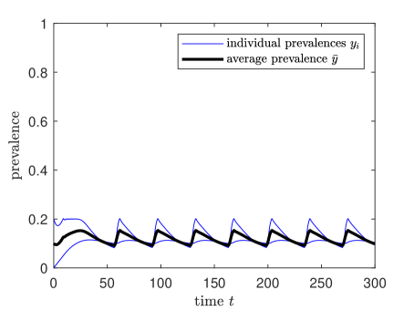
(a) Local and average prevalence.

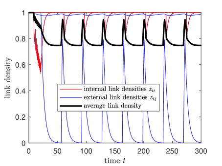
(b) Link densities.

Figure 1: Case study 1: effect of asymmetric response between two communities. Parameters are $n=2$, $\beta_{ij}\sim U([0,1.2]),\delta_{i}=U([0,0.5]),\zeta_{ij}\sim U([0,1]),\xi_{ij}\sim U([0,1])$ for $i,j=1,2$, where $U$ denotes the uniform distribution. (a) local and average prevalence; (b) link densities. We observe a quick convergence towards a stable limit cycle, representing endemicity of the disease alternating between high and low prevalence in the population.

We consider system (2) on a small network of $n=2$ communities, and consider an asymmetry in the functional responses between the two communities. We assume identical internal policies:

$$f_{\textnormal{cr,ii}}(y_{i},\bar{y})=\mathbbm{1}_{\{y_{i}\leq 0.2\}},\quad f_{\textnormal{br,ii}}(y_{i},\bar{y})=\mathbbm{1}_{\{y_{i}>0.2\}},\quad i=1,2,$$

meaning a strict lockdown is imposed within each community as soon as the internal prevalence exceeds a threshold value of $0.2$, regardless of the average global prevalence. Oppositely, we assume that connections between the two communities are governed by asymmetrical rules:

$$f_{\text{cr},12}(y_{1},y_{2},\bar{y})=\mathbbm{1}_{\{y_{2}\leq 0.1\}},\quad f_{\text{br},12}(y_{1},y_{2},\bar{y})=\mathbbm{1}_{\{y_{2}>0.1\}},$$

$$f_{\text{cr},21}(y_{1},y_{2},\bar{y})=1-y_{1}y_{2},\quad f_{\text{br},21}(y_{1},y_{2},\bar{y})=y_{1}y_{2}.$$

This choice results, for values of the parameters corresponding to $R_{0}\approx 1.33$, in local and average prevalence, as well as all the link densities, quickly approaching stable limit cycles, as illustrated in Figure 1.

This asymmetry can be interpreted as community 1 being the “hub” in this network of communities, and community 2 being a peripheral node. The same behaviour can be observed with bigger communities, for example a star network of $n\geq 3$ communities with asymmetric responses between hub and peripheral nodes and vice versa. However, the simplest case of $n=2$ presented in Figure 1, which corresponds to a system of only six ODEs, perfectly exemplifies the potential of our modelling approach in producing complex behaviour starting from a simple SIS epidemic model.

Even though the provided functional responses contain indicator functions, which are not $\mathcal{C}^{1}$-functions over the interval $[0,1]$, we emphasise that other choices of $f_{\text{cr,ii}}$, $f_{\text{br,ii}}$, $f_{\text{cr,ij}}$ and $f_{\text{br,ij}}$ can also lead to periodic behaviour. The benefit of having $\mathcal{C}^{1}$-functions is that the solution is guaranteed to be unique. One method is to approximate the indicator function, for which we verified that periodic solutions also occur.

Lastly, we remark that the existence of limit cycles is completely independent of the dependence of awareness on the global prevalence $\bar{y}$. We investigate the influence of the dependence on the global prevalence in Section 4.4.

4.2 Case study 2: Seasonality

Besides periodic behaviour emerging naturally from the multigroup aNIMFA model, it is natural for infectious diseases to exhibit seasonal dependency. In particular, the flu is known to resurface in the colder months, because of the reduced functioning of the immune system and the increased crowding inside buildings. The natural periodicity therefore appears through the infection rates $\beta_{ij}$ with period $T$. The collective behaviour of a population usually changes gradually throughout the year and slowly follows the temperature changes. However, modelling abrupt (i.e. discontinuous) changes can be of interest as well, especially considering the possibility of overnight introduction or lifting of lockdown measures, which have been a significant part of the containment strategy of COVID-19 in various nations.

As periodic functions we utilise the sine wave and the block wave with period $T$;

$$f(t) =\sin^{2}\left(\frac{\pi t}{T}\right)$$ (13a)

$$f(t) =4\left\lfloor\frac{t}{T}\right\rfloor-2\left\lfloor\frac{2t}{T}\right\rfloor+1$$ (13b)

Consider a complete network of $n=20$ communities, that is, all communities are assumed to be connected to all other communities. A disease emerges emerges in community 1 at time $t=0$, which translates into the initial conditions $y_{1}(0)=0.2$ and $y_{i}(0)=0$ for all other communities $i$. The initial link density $z_{ij}(0)=1$ for all communities $i$. Each community is assumed to have only local awareness, i.e. the link-breaking and link-creation mechanisms are independent of the global prevalence $\bar{y}$. For the link-creation mechanism, we propose

$$\begin{split}f_{\textnormal{cr,ii}}&=1-y_{i}^{2},\\ f_{\textnormal{cr,ij}}&=1-y_{i}y_{j},\end{split}$$ (14)

and for the link-breaking mechanism, we pick

$$\begin{split}f_{\textnormal{br,ii}}&=y_{i}^{2},\\ f_{\textnormal{br,ij}}&=y_{i}y_{j}.\end{split}$$ (15)

We quantify the impact of the periodic functions on the size of the epidemic outbreak based on two parameters: the global prevalence in the steady state $\bar{y}_{\infty}$ and the peak prevalence $y_{p}$, which is the maximal prevalence over all times and all communities:

$$y_{p}:=\max_{\begin{subarray}{c}0\leq t\leq\infty\\ i=1,...,n\end{subarray}}y_{i}(t)$$

Figure 2 demonstrates the prevalence for each of the periodic infection rates from Eq. (13). Figure 2 depicts that a block wave is more devastating than a sine wave in terms of the peak prevalence. In other words, a sudden uprising and disappearance of a disease is much more dangerous than gradual outbreaks. For sudden uprisings, people cannot respond to the disease sufficiently fast and a large outbreak is inevitable. Therefore, timely communication from governments and health agencies is crucial to mitigate dangerous epidemic outbreaks.

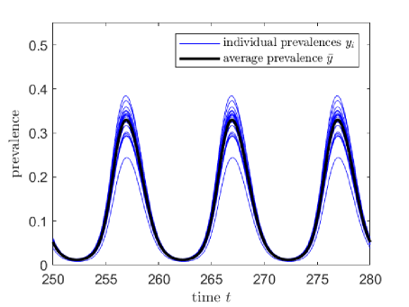
(a) Sine wave

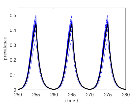
(b) Block wave

Figure 2: Case study 2: effect of seasonality on the prevalence in terms of a time-periodic infection rate with period $T=10$ using (a) a sine wave and (b) a block wave. Parameters are $n=20$, $\beta_{ij}\sim U([0,0.25]),\delta_{i}=1,\zeta_{ij}\sim U([0,2]),\xi_{ij}\sim U([0,1])$ for all $i,j$, where $U$ denotes the uniform distribution. The basic reproduction number $R_{0}=2.53$ for $f(t)=1$.

We further quantify the differences between sine and block waves in terms of the average prevalence over one period and the peak prevalence. Figure 3 depicts the dependence of the properties on the period $T$. The black, dashed baseline in Figure 3 corresponding to $f(t)=0.5$ is equal to the average over one period of the periodic functions, i.e. the total force of infection is assumed to be constant. Figure 3 indeed shows that the block waves are the most disastrous in terms of the peak prevalence, for any period $T$. Moreover, longer time periods result in more severe pandemics in terms of the peak prevalence, because during a long period of high infectiousness, the disease can spread, but the network cannot adapt sufficiently fast, leading to higher prevalence values. On the other hand, the average prevalence over one period appears to decrease due to long periods of inactivity.

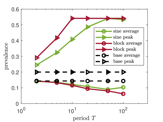
Figure 3: Case study 2: impact of the period $T$ on the steady-state prevalence $\bar{y}_{\infty}$ and the peak prevalence $y_{p}$ for sine waves (green) and block waves (red) for the peak prevalence (triangle) and average prevalence (circle). Parameters are the same as Figure 2.

We now investigate the seasonal behaviour for two types of networks: the Barbell graph (two complete graphs connected by a single edge; see Figure 4 for a visualization) and the star graph (see Figure 6 for a visualization).

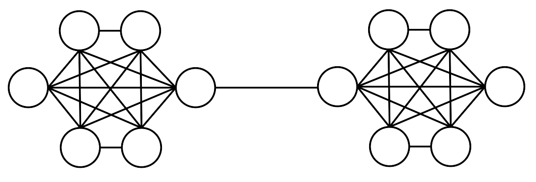
Figure 4: Barbell graph with 12 nodes.

With the same parameters and choice of periodic functions as in Figure 2, the Barbell graph shows disease persistence with $R_{0}>1$, leading to periodic behavior. For the Barbell graph, Figure 5 illustrates that periodic behavior appears immediately, and changing the response function (i.e., from sine to block wave) results in a similar peak prevalence. However, the wave generated with the block function is peculiar: after the peak, there is an initial slow decline followed by a steeper decline. This distinct behavior can be attributed to the structure of the Barbell graph. The Barbell graph consists of two cliques connected by one or more bridging nodes. Without loss of generality, in our case we consider only one bridge node.

When the disease initially starts in one of the cliques, the high connectivity within the clique causes a rapid initial spread, leading to an overshoot in the initial prevalence. This initial overshoot is because the dense connections within the clique facilitate a swift transmission of the disease, causing the number of infected individuals to rise quickly. As the disease spreads through the bridge node to the second clique, the overall prevalence reaches its peak. The subsequent decline in the number of infected individuals is initially slow due to the high number of connections within each clique, which sustains the transmission for a longer period within the clique before the disease starts to die out. Once the disease prevalence in the first clique significantly reduces, the decline becomes steeper as the disease runs out of susceptible individuals to infect. The second, faster and steeper decline is caused by the switching “off” of the block wave. The abrupt change in the response function results in an exponential convergence towards zero prevalence, i.e., the Disease-Free Equilibrium (DFE). Finally, the subsequent switching “on” before reaching the DFE, which only happens asymptotically as $t\to+\infty$, allows for a rapid increase in infection again.

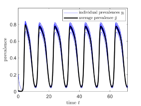
(a) Sine wave

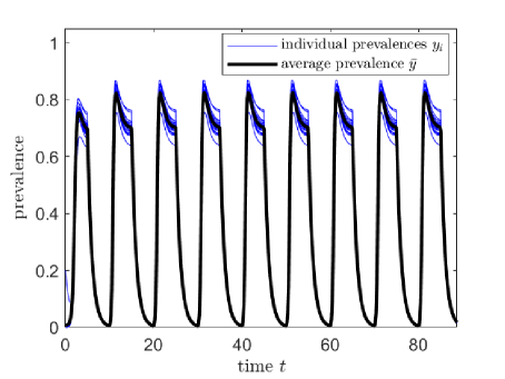
(b) Block wave

Figure 5: Case study 2: effect of seasonality on the prevalence in terms of a time-periodic infection rate with period $T=10$ using (a) a sine wave and (b) a block wave for a Barbell graph on $n=20$ nodes. The parameters and functional responses are the same as the complete network, which correspond to $R_{0}=9.59$.

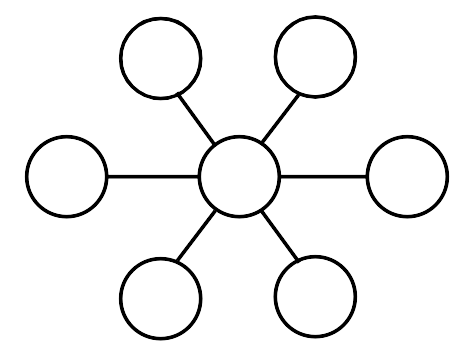
Figure 6: Star graph with 7 nodes.

For the star graph (visualized in Figure 6), using the parameters from Section 4.2 results in $R_{0}<1$, consequently leading directly to extinction of the epidemic. By slightly altering the parameters, we find that the star graph in Figure 7 exhibits periodic waves similar to those of the complete graph; however, the peaks in the hub community appear to dominate the peaks of all other nodes. After all, the hub is connected to all other nodes and has therefore the most chance of getting infected.

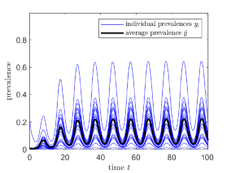
(a) Sine wave

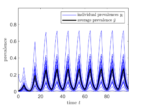
(b) Block wave

Figure 7: Case study 2: effect of seasonality on the prevalence in terms of a time-periodic infection rate with period $T=10$ using (a) a sine wave and (b) a block wave for the star graph on $n=20$ nodes. The functional responses are the same as in the complete network, with the parameters $\beta_{ij}\sim U([0,1]),\delta_{i}=1,\zeta_{ij}\sim U([0,2]),\xi_{ij}\sim U([0,1])$ for all $i,j$, where $U$ denotes the uniform distribution. The basic reproduction number $R_{0}=2.99$.

4.3 Case study 3: Internal and external connections

To mitigate epidemics, policy-makers have several tools available. In the early phases of an epidemic, in which vaccines and drugs are still unavailable, only Non-Pharmaceutical Interventions (NPIs) can be utilised. Link-breaking policies are an important part of these NPIs. It is, however, not immediately clear whether it is preferable to remove connections within or between communities. By including a parameter in the system which weighs the relative magnitude of the corresponding response functions, we model a range of possible scenarios, ranging from total internal awareness and adaptivity (i.e., containment measures are taken within each community) to completely total external awareness (i.e., containment measures are taken between each couple of connected communities). We do so by considering the following choice for our functions:

$$\begin{split}f_{\textnormal{br,ii}}&=cy_{i}^{2},\\ f_{\textnormal{br,ij}}&=\frac{1}{c}y_{i}y_{j}.\end{split}$$ (16)

The constant $c$ allows for the balancing of the importance of internal and external responses to the epidemic. For $c=1$, the link-breaking functional response for external and internal connections is equivalent. Otherwise, for $c>1$, links are broken at a higher rate within communities and for $c<1$, links are broken at a higher rate between communities. The remainder of the parameters as well as the complete graph are equivalent to Case Study 2. Figure 8 depicts the time-evolving prevalence and link densities for three different situations. As expected, high link-breaking rates within communities results in less links within communities, and vice versa.

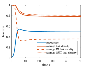
(a) Mainly break within communities

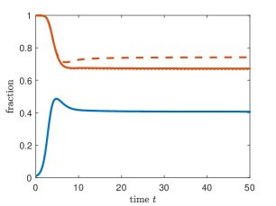
(b) Balanced situation

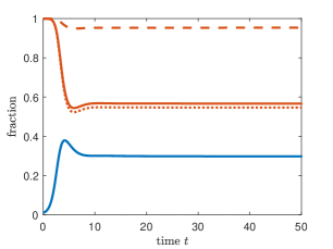
(c) Mainly break between communities

Figure 8: Case study 3: influence of breaking within or between communities on the prevalence and link densities. The parameters and functional responses are the same as in Case study 2 with a complete network, resulting in $R_{0}=2.53$, with the exception that we used for (a), $c=4$, for (b), $c=1$ and for (c), $c=0.25$.

Figure 8 also suggests that breaking connections between communities may be preferable compared to breaking connections within communities to reduce the epidemic outbreak. We quantify the effectiveness of all methods using the peak prevalence $y_{p}$ and the steady-state prevalence $\bar{y}_{\infty}$.

Figure 9a confirms for a wide range of $c$-values that breaking connections between communities is more successful in reducing the epidemic outbreak size than breaking connections within communities. We emphasise that this conclusion is highly dependent on the choice of the functional responses as well as the topology; different choices may result in significantly different behaviour.

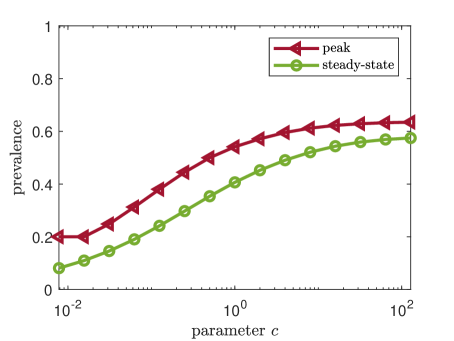
(a) complete graph

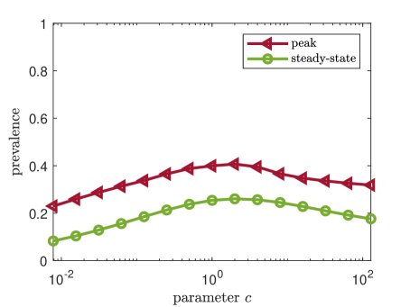
(b) cycle graph

Figure 9: Case study 3: impact of the parameter $c$ on the steady-state prevalence $\bar{y}_{\infty}$ and the peak prevalence $y_{p}$ in the (a) complete graph and (b) cycle graph. Parameters are the same as Figure 8, except for (b), we have chosen $\beta_{ij}\sim U([0,1])$, such that $R_{0}=1.83$. The horizontal axis is shown on a logarithmic scale.

In particular, when considering a cycle graph, where each community is only connected to its two nearest neighbours, the situation changes drastically as observed in Figure 9b. Compared to the balanced situation $c=1$ where links are broken equally fast within and between communities, both extremes $c\to 0$ and $c\to\infty$ appear to be beneficial for reducing the spread. Most likely, the spread of the disease can be diminished by one of two methods: (i) isolating communities with many infections or (ii) preventing getting infected by breaking connections between communities. This contrasts our results for the all-to-all topology in Figure 9a, where the method of quarantining communities (i.e. breaking links within communities) does not work very well, because of the huge number of neighbouring communities. Overall, we conclude that a cycle network is more localised and quarantining is therefore more effective than on the complete network.

4.4 Case study 4: Local versus global awareness

Besides the influence of external and internal functional responses and the periodicity, another key aspect of the aNIMFA model is the possible dependence of the functional responses on the local and global prevalence, i.e. the choice for breaking and creating links can be dependent on the local and global information on the disease.

As in case study 2 and 3, the link-creation functional responses are taken as

$$\begin{split}f_{\textnormal{cr,ii}}&=1-y_{i}^{2},\\ f_{\textnormal{cr,ij}}&=1-y_{i}y_{j},\end{split}$$ (17)

and for the link-breaking mechanism, we pick

$$\begin{split}f_{\textnormal{br,ii}}&=y_{i}^{2},\\ f_{\textnormal{br,ij}}&=c\ y_{i}y_{j}+(1-c)\ \bar{y}^{2}.\end{split}$$ (18)

Here, the constant $c$ balances between the breaking of links based on completely local information ($c=1$) and completely global information ($c=0$).

We emphasise that considering the global prevalence to make decisions whether to break connections is fundamentally different to taking all-to-all couplings. In a complete graph, the prevalence of all nodes influence a node’s prevalence, whereas global awareness uses the average of all node prevalences to influence the link density directly, but cannot influence the node’s prevalence directly.

For many graphs, graph sizes, functional responses and homogeneous and heterogeneous parameters, the peak prevalence $y_{p}$ and the steady-state prevalence $\bar{y}_{\infty}$ are the highest with only global awareness ($c=0$) and decrease monotonically with increasing $c$. This is exemplified in Figure 10b in a Barabási-Albert graph [31]. The reasoning is as follows. Even though using global information may prevent spreading in some links on the network, it is only an average, necessarily also resulting in less link removals between other communities. Especially the most vulnerable parts of the network, i.e. those nodes with few infections and high neighbouring infections, have the most benefit by considering their neighbours directly instead of information on the network as a whole. In total, we can only conclude that local information is superior to suppress an epidemic for links between communities.

In another closely related scenario, we also balance between local and global awareness, but now for the internal link densities $z_{ii}$, which changes the link-breaking mechanisms to

$$\begin{split}f_{\textnormal{br,ii}}&=c\ y_{i}^{2}+(1-c)\ \bar{y}^{2},\\ f_{\textnormal{br,ij}}&=y_{i}y_{j}.\end{split}$$ (19)

When a community with low prevalence is connected to a community with high prevalence, precautiously removing links within its own community may help to reduce the spread of the disease. Figure 10a supports our hypothesis by demonstrating that the steady-state prevalence $\bar{y}_{\infty}$ may exhibit non-monotonic behaviour in the parameter $c$. The effect of the parameter $c$ is admittedly small, but we believe the effect can be more substantial in larger networks. To conclude, for link removals within communities, there is no superior strategy – depending on the network structure, the severity of the disease and the network dynamics, using global information may help to reduce the spreading of the disease. We expect that global information will become more important in larger networks, which we leave as a direction for further research.

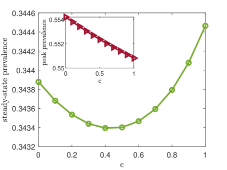
(a) Within communities

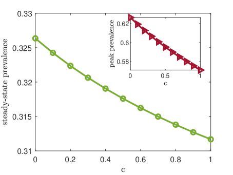
(b) Between communities

Figure 10: Case study 4: balancing between local and global awareness of the disease (a) within communities and (b) between communities showing the peak prevalence (red triangles) and the steady-state prevalence (green circles). All curves are declining for increasing $c$ values, but the steady-state prevalence within communities is non-monotonic. Simulations are based on an Barabási-Albert graph with $m_{0}=3,m=2$, $\delta_{i}=1,\zeta_{ij}\sim U([0,2]),\xi_{ij}\sim U([0,1])$, $y_{i}(0)=0$ for all $i\neq 1$ and $y_{1}(0)=0.2$ and $z_{ij}(0)=0$ for all $i,j$. Furthermore, (a) $n=20$ nodes, $\beta_{ij}\sim U([0,1])$ such that $R_{0}=2.93$ and (b) $n=50$ nodes, $\beta_{ij}\sim U([0,0.8])$ such that $R_{0}=2.60$.

5 Conclusions

In this paper, we proposed a generalization of the aNIMFA model investigated in [1] to a network of $n$ communities. We provided a formula for the well-known basic reproduction number $R_{0}$. We investigated existence and stability of equilibria of the system. As usual with this type of models, the stability of the Disease Free Equilibrium depends the threshold value $R_{0}$ being smaller or greater than $1$. We also showed that at least one Endemic Equilibrium exists under a condition slightly stronger than $R_{0}>1$.

Lastly, we enhanced our analytical results through an extensive numerical exploration of various case studies. In particular, we showed that the multigroup aNIMFA model allows for periodic orbits in a network with just two communities. We showcased this fact with an asymmetric on/off strategy for the adaptivity between communities, representing total lockdowns when the prevalence reaches a given threshold. Moreover, we investigated the effect of a seasonally-varying infection rate on the prevalence by comparing multiple kinds of networks. Then we showed that breaking connections between communities is preferable over breaking connections within communities in dense graphs, but in sparse networks (with few links) both link-breaking strategies are viable approaches to lessen the disease prevalence. Lastly, we measured the trade-off between local and global awareness on the current state of the epidemic. In many scenarios, using local information appears superior to using global awareness, but further research on larger networks is required to fully support this claim.

Given that many of our conclusions are drawn based on numerical solutions, it would be interesting to derive an analytical foundation of these results, while keeping restrictions on the functional responses $f_{\textnormal{br,ij}}$ and $f_{\textnormal{cr,ij}}$ as minimal as possible. Perhaps monotonicity of the functional responses is sufficient to deduce information on the asymptotic behaviour of the system. Or is there any other characteristic one could leverage to foresee relevant characteristics of the system, e.g. the peak of prevalence or the steady-state prevalence?

Moreover, we remark that our approach to the modelling of adaptivity in the context of epidemic spreading can be easily generalized to more complex models. The main underlying hypothesis of the systems presented here and in [1] is the SIS compartmental structure, which does not allow for any kind of immunity. However, modelling the connectivity based on link densities between between nodes and viral states can be included in any multigroup model, as a level of adaptation of the communities to the evolution of an epidemic. In more complex models, such as the SIR (Susceptible – Infected – Recovered), SIRS, SAIRS (Susceptibel – Asymptomatic – symptomatic Infectious – Recovered – Susceptible) or SIRWS (Susceptible – Infectious – Recovered – Waning immunity – Susceptible), incorporating disease awareness and adaptivity in the system is crucial for improving its realism. Our approach to the subject is very simple, and therefore well-suitable for wide applicability in epidemics.

Acknowledgements. Mattia Sensi was supported by the Italian Ministry for University and Research (MUR) through the PRIN 2020 project “Integrated Mathematical Approaches to Socio-Epidemiological Dynamics” (No. 2020JLWP23, CUP: E15F21005420006).

References

- [1] M. A. Achterberg and M. Sensi. A minimal model for adaptive SIS epidemics. Nonlinear Dynamics, 111:12657–12670, 2023.
- [2] D. Juher, D. Rojas, and J. Saldaña. Robustness of behaviorally induced oscillations in epidemic models under a low rate of imported cases. Physical Review E, 102(5):052301, 2020.
- [3] D. Juher, D. Rojas, and J. Saldaña. Saddle–node bifurcation of limit cycles in an epidemic model with two levels of awareness. Physica D: Nonlinear Phenomena, 448:133714, 2023.
- [4] W. Just, J. Saldaña, and Y. Xin. Oscillations in epidemic models with spread of awareness. Journal of Mathematical Biology, 76(4):1027–1057, 2018.
- [5] F. D. Sahneh and C. M. Scoglio. Optimal information dissemination in epidemic networks. In 2012 IEEE 51st IEEE conference on decision and control (cdc), pages 1657–1662. IEEE, 2012.
- [6] F. D. Sahneh, A. Vajdi, J. Melander, and C. M. Scoglio. Contact Adaption During Epidemics: A Multilayer Network Formulation Approach. IEEE Transactions on Network Science and Engineering, 6(1):16–30, 2019.
- [7] E. Agliari, R. Burioni, D. Cassi, and F. M. Neri. Efficiency of information spreading in a population of diffusing agents. Physical Review E, 73(4):046138, 2006.
- [8] S. Funk, E. Gilad, C. Watkins, and V. A. A. Jansen. The spread of awareness and its impact on epidemic outbreaks. Proceedings of the National Academy of Sciences, 106(16):6872–6877, 2009.
- [9] A. Szabó-Solticzky, L. Berthouze, I. Z. Kiss, and P. L. Simon. Oscillating epidemics in a dynamic network model: stochastic and mean-field analysis. J. Math. Bio., 72:1153–1176, 2016.
- [10] R. Kouzy, J. Abi Jaoude, A. Kraitem, M. B. El Alam, B. Karam, E. Adib, J. Zarka, C. Traboulsi, E. W. Akl, and K. Baddour. Coronavirus Goes Viral: Quantifying the COVID-19 Misinformation Epidemic on Twitter. Cureus, 12, 2020.
- [11] T. Gross, C. J. D. D’Lima, and B. Blasius. Epidemic dynamics on an adaptive network. Phys. Rev. Lett., 96:208701, May 2006.
- [12] I. Z. Kiss, L. Berthouze, T. J. Taylor, and P. L. Simon. Modelling approaches for simple dynamic networks and applications to disease transmission models. Proc. R. Soc. A, 468:1332–1355, 2012.
- [13] M. A. Achterberg, J. L. A. Dubbeldam, C. J. Stam, and P. Van Mieghem. Classification of link-breaking and link-creation updating rules in susceptible-infected-susceptible epidemics on adaptive networks. Phys. Rev. E, 101:052302, May 2020.
- [14] J. Cascante-Vega, S. Torres-Florez, J. Cordovez, and M. Santos-Vega. How disease risk awareness modulates transmission: coupling infectious disease models with behavioural dynamics. Royal Society Open Science, 9(1):210803, 2022.
- [15] A. Lajmanovich and J. A. Yorke. A deterministic model for gonorrhea in a nonhomogeneous population. Mathematical Biosciences, 28(3):221–236, 1976.
- [16] W. Huang, K. L. Cooke, and C. Castillo-Chavez. Stability and bifurcation for a multiple-group model for the dynamics of HIV/AIDS transmission. SIAM Journal on Applied Mathematics, 52(3):835–854, 1992.
- [17] R. Sun and J. Shi. Global stability of multigroup epidemic model with group mixing and nonlinear incidence rates. Applied Mathematics and Computation, 218(2):280–286, 2011.
- [18] Y. Muroya, Y. Enatsu, and T. Kuniya. Global stability for a multi-group SIRS epidemic model with varying population sizes. Nonlinear Analysis: Real World Applications, 14(3):1693–1704, 2013.
- [19] Y. Muroya and T. Kuniya. Further stability analysis for a multi-group SIRS epidemic model with varying total population size. Applied Mathematics Letters, 38:73–78, 2014.
- [20] R. N. Mohapatra, D. Porchia, and Z. Shuai. Compartmental disease models with heterogeneous populations: a survey. In Mathematical Analysis and its Applications: Roorkee, India, December 2014, pages 619–631. Springer, 2015.
- [21] D. Fan, P. Hao, D. Sun, and J. Wei. Global stability of multi-group SEIRS epidemic models with vaccination. International Journal of Biomathematics, 11(01):1850006, 2018.
- [22] M. Adimy, A. Chekroun, L. Pujo-Menjouet, and M. Sensi. A multigroup approach to delayed prion production. Discrete and Continuous Dynamical Systems-B, 29(7):2972–2998, 2024.
- [23] S. Ottaviano, M. Sensi, and S. Sottile. Global stability of multi-group SAIRS epidemic models. Mathematical Methods in the Applied Sciences, 46(13):14045–14071, 2023.
- [24] S. Boccalini, E. Pariani, G. E. Calabrò, C. De Waure, D. Panatto, D. Amicizia, P. L. Lai, C. Rizzo, E. Amodio, F. Vitale, et al. Health technology assessment (HTA) of the introduction of influenza vaccination for Italian children with Fluenz Tetra®. Journal of Preventive Medicine and Hygiene, 62(2):E1–E118, 2021.
- [25] G. E. Calabrò, S. Boccalini, A. Bechini, D. Panatto, A. Domnich, P. L. Lai, D. Amicizia, C. Rizzo, A. Pugliese, M. L. Di Pietro, et al. Health Technology Assessment: a value-based tool for the evaluation of healthcare technologies. reassessment of the cell-culture-derived quadrivalent influenza vaccine: Flucelvax Tetra® 2.0. Journal of preventive medicine and hygiene, 63(4/Supplement 1):E1–E140, 2022.
- [26] A. Fochesato, S. Sottile, A. Pugliese, S. Márquez-Peláez, H. Toro-Diaz, R. Gani, P. Alvarez, and J. Ruiz-Aragón. An economic evaluation of the adjuvanted quadrivalent influenza vaccine compared with standard-dose quadrivalent influenza vaccine in the spanish older adult population. Vaccines, 10(8):1360, 2022.
- [27] P. Van Mieghem. The N-intertwined SIS epidemic network model. Computing, 93:147–169, Dec 2011.
- [28] P. Van den Driessche and J. Watmough. Further notes on the basic reproduction number. Mathematical epidemiology, pages 159–178, 2008.
- [29] W. Kulpa. The Poincaré-Miranda theorem. The American Mathematical Monthly, 104(6):545–550, 1997.
- [30] J. Mawhin. Simple proofs of the Hadamard and Poincaré–Miranda theorems using the Brouwer fixed point theorem. The American Mathematical Monthly, 126(3):260–263, 2019.
- [31] A. Barabási. Network science. Cambridge University Press, Cambridge, United Kingdom, Jul 2016.