On the sensitivity of nuclear clocks to new physics

Abstract

The recent demonstration of laser excitation of the $\approx 8$ eV isomeric state of thorium-229 is a significant step towards a nuclear clock. The low excitation energy likely results from a cancellation between the contributions of the electromagnetic and strong forces. Physics beyond the Standard Model could disrupt this cancellation, highlighting nuclear clocks’ sensitivity to new physics. Accurate predictions of the different contributions to nuclear transition energies, and therefore of the quantitative sensitivity of a nuclear clock, are challenging. We improve upon previous sensitivity estimates and assess a “nightmare scenario,” where all binding energy differences are small and the new physics sensitivity is poor. A classical geometric model of thorium-229 suggests that fine-tuning is needed for such a scenario. We also propose a $d$-wave halo model, inspired by effective field theory. We show that it reproduces observations and suggests the “nightmare scenario” is unlikely. We find that the nuclear clock’s sensitivity to variations in the effective fine structure constant is enhanced by a factor of order $10^{4}$. We finally propose auxiliary nuclear measurements to reduce uncertainties and further test the validity of the halo model.

1 Introduction

Roughly 80% of the matter content of our Universe consists of dark matter (DM). Despite ample evidence for its existence from astrophysical and cosmological observations, little is known about its nature, and it is considered to be one of the greatest mysteries of contemporary physics. Theories of ultralight dark matter (ULDM) bosons (scalar or pseudo-scalar) provide us with arguably the simplest explanation for its nature. Well-motivated models of ULDM include the axion [1, 2, 3, 4, 5] of quantum chromodynamics (QCD), the dilaton [6] (though see Ref. [7]), the relaxion [8, 9], and possibly other forms of Higgs-portal models [10]. Finally, it was recently shown that the Nelson–Barr framework that also addresses the strong-CP problem, leads to a viable ULDM candidate [11]. All of these models predict that the ULDM would couple dominantly to the Standard Model (SM) QCD sector, the quarks and the gluons, leading to oscillations of nuclear parameters [12, 13, 14]. These models would also lead to subdominant coupling to the QED sector via time variation of $\alpha_{\text{em}}$, the fine structure constant. Scalar ULDM generically couples linearly to the hadron masses (see [15] for a recent review), whereas pseudo-scalars (axions) couple quadratically [16] (though see Ref. [17, 18]). Furthermore, one can construct a broad class of natural ULDM models where the leading DM interaction with the SM fields is quadratic [19]. All of these lead to oscillation of the nuclear/hadronic parameters.

Variations of SM parameters can be searched for by comparing the rates of two clocks (e.g., quantum transitions or resonators) that exhibit different dependence on the parameters in question [14, 6, 20]. Laboratory limits on these variations have been obtained from various clock-comparison experiments based on atomic or molecular spectroscopy as well as cavities and mechanical oscillators. However, these experimental probes mostly rely on electronic transitions, whereas their sensitivity to changes in the nuclear sector is largely suppressed. Hyperfine transitions and mechanical oscillators, (Cs clock, hydrogen maser, quartz oscillator) [21, 22, 23, 24, 25, 26], which are sensitive to variation of the nuclear parameters, do not reach the accuracy and stability of optical clocks. In optical clocks nuclear properties enter via hyperfine structure and the reduced mass, but their relative contributions are typically only of order $10^{-6}$ and $10^{-5}$, respectively. The contributions from the oscillation of the charge radius, is around $10^{-3}$ [27]. Rovibrational transitions in molecules promise an $\mathcal{O}(1)$ sensitivity to a modulation of nuclear parameters [28, 29], although current constraints only exist at modulation frequencies above $10\text{\,}\mathrm{Hz}$ [30].

This is one of two main reasons for why a nuclear clock, which precisely monitors an ultra-narrow nuclear transition, could lead to a quantum leap in ULDM searches,  [31, 32, 33, 34]. The only isotope known to possess a suitable clock-nuclear transition is ²²⁹$\rm Th$, which features an isomeric state, ${}^{229\text{m}}$$\rm Th$, a mere $8\text{\,}\mathrm{e}\mathrm{V}$ above the ground state, low enough to be excitable with a laser [35, 36] (for illustration see Fig. 1). In fact, laser excitation of this transition has recently been reported for the first time [37, 38, 39]. This constitutes a major breakthrough on the way towards a nuclear clock, which is hoped to surpass the frequency stability of even the best atomic clock, given that the nucleus is better shielded from environmental noise than the electron shell. Regarding searches for physics beyond the SM, line-shape analysis of the ²²⁹$\rm Th$ data would lead to world-record sensitivity already now, well before a nuclear clock is going to be realized [40].

The second reason for why the nuclear clock might be extremely sensitive to the presence of new physics is due to an accidental cancellation between the nuclear energy shift and the electromagnetic energy shift compared to the ground state, which results in the observed small transition energy. New physics that couples differently to either of these contributions disrupts this cancellation. A nuclear clock is therefore believed to have spectacular sensitivity to certain classes of physics beyond the SM, naively being of the order of $\,$\mathrm{M}\mathrm{e}\mathrm{V}$/10\,$\mathrm{e}\mathrm{V}$\sim 10^{5}$. The sensitivity of a nuclear clock to physics beyond the SM has been explored in a number of papers (see for example [41, 42, 43, 44, 45, 46, 47]). Recent reviews can be found in Refs. [15, 48, 49].

However, to accurately quantify this sensitivity, the degree of fine-tuning in the transition energy (or, in other words, the absolute magnitude of the electromagnetic or nuclear energy difference between the ground state and the isomer) needs to be known. This is hindered by intrinsic imperfection in all models of atomic nuclei. At the moment, as we will see below, even a “nightmare scenario” where no cancellation occurs (and the electromagnetic and nuclear energy differences happen to be at the eV scale individually) cannot be ruled out. This would leave the nuclear clock with a disappointing enhancement factor of $\mathcal{O}(1)$.

Our goal in the present paper is to quantify how likely this nightmare scenario is. We do so by calculating the Coulomb energy difference between the ground state and the isomer of ²²⁹$\rm Th$ first in a classical, geometric, model of the nucleus, parameterized by its charge radius, quadrupole and higher moments, as well as the skin thickness (Section 2.1). We then derive similar results using a quantum halo model, in which ²²⁹$\rm Th$ is described as a ²²⁸$\rm Th$ core orbited by a halo neutron, and the two states differ in the spin alignment of the halo neutron (Section 2.2). Finally, in Section 3, we conclude and propose a number of auxiliary measurements and further steps that could shed more light on the likelihood of the nightmare scenario and the sensitivity of a nuclear clock to physics beyond the SM.

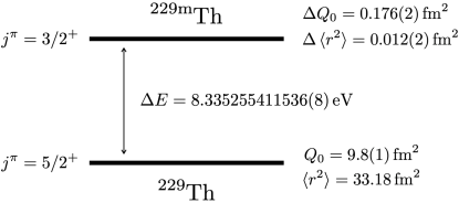
Figure 1: Illustration of nuclear level properties, namely excitation energy $\Delta E$ [35, 36], intrinsic electric quadrupole momentum $Q_{0}$  [50, 39] and mean squared charge radius $\langle r^{2}\rangle$  [50, 51, 42], of the almost-degenerate ground-state ²²⁹$\rm Th$ and isomer ${}^{229\text{m}}$$\rm Th$.

2 The $\mathbf{{{}^{229}\rm\bf Th}}$ Nucleus

²²⁹Th is a heavy nucleus. This trivial fact makes its modeling from first principles problematic. The problem intensifies when considering the isomeric state, whose energy difference with the ground state, $\Delta E=$8.335\,255\,411\,536(8)\text{\,}\mathrm{e}\mathrm{V}$$ [39], lies far below typical nuclear physics scales. As mentioned before, the presumed explanation for this unnaturally low scale is a cancellation between the electromagnetic contribution, $\Delta E_{\text{em}}$, and the nuclear contribution, $\Delta E_{\text{nuc}}$, to the transition energy,

$$\Delta E=\Delta E_{\text{em}}+\Delta E_{\text{nuc}}\,,$$ (1)

where very naively we expect $\big{|}\Delta E_{\text{em}}\big{|}\sim\big{|}\Delta E_{\text{nuc}}\big{|}\gg\Delta E\,.$ Physics beyond the SM may affect one of these contributions, but not the other, thereby breaking the fine-tuned cancellation.

The conventional lore is that this implies a sensitivity that is enhanced compared to the sensitivity of an optical lattice clock by a factor of $\big{|}\Delta E_{\text{em}}\big{|}/\Delta E\simeq\big{|}\Delta E_{\text{nuc}}\big{|}/\Delta E$. To compute the enhancement factor, determine the sensitivity of a ${}^{229\text{m}}$$\rm Th$ nuclear clock to new physics, and interpret measurements in this context, it is necessary to determine $\Delta E_{\text{em}}$ independently. As $\Delta E_{\text{em}}$ is not an observable, and at present cannot be computed from first principles, this requires modelling.

More precisely, if physics beyond the SM manifests itself as an effective variation of the strong coupling constant, $\delta\alpha_{s}$, and/or an effective variation of the electromagnetic coupling constant, $\delta\alpha_{\text{em}}$, (for instance due to dark matter oscillations), we can use Eq. (1) to write the corresponding variation of the transition energy as

$$\frac{\delta(\Delta E)}{\Delta E}=\frac{1}{\Delta E}\bigg{(}\frac{\partial\Delta E_{\text{em}}}{\partial\alpha_{\text{em}}}\delta\alpha_{\text{em}}+\frac{\partial(\Delta E_{\text{em}}+\Delta E_{\text{nuc}})}{\partial\alpha_{s}}\delta\alpha_{s}\bigg{)}\,,$$ (2)

where in Eq. 2 we have used the fact that $\partial(\Delta E_{\text{em}}+\Delta E_{\text{nuc}})/\partial\alpha_{\text{em}}=\partial\Delta E_{\text{em}}/\partial\alpha_{\text{em}}$. In case of a time varying background they would become accessible for quantum sensors, contrary to $\Delta E_{\text{em}}$ and $\Delta E_{\text{nuc}}$ themselves.

Dark matter-induced variations of $\alpha_{\text{em,s}}$ are typically of the form $\delta\alpha_{\text{em},\text{s}}=\alpha_{\text{em},\text{s}}(1+\mathcal{F}(t)g_{\text{em},\text{s}})\,,$ where $g_{\text{em},\text{s}}$ denotes the dark matter coupling strength to either the electromagnetic or strong sector of the SM, while $\mathcal{F}(t)$ is a function which depends on the dark matter energy density and mass, with the latter setting the frequency at which $\mathcal{F}(t)$ oscillates.

In the following we focus on the computation of the electromagnetic enhancement factor, defined as

$$K_{\text{em}}\equiv\frac{1}{\Delta E}\frac{\partial\Delta E_{\text{em}}}{\partial\log\alpha_{\text{em}}}\simeq\frac{\Delta E_{\text{em}}}{\Delta E}\,,$$ (3)

where in the last equality we have assumed that $\Delta E_{\text{em}}$ depends linearly on $\alpha_{\text{em}}$. Any other power-law dependence will give an order-one correction which is irrelevant for the scope of this work. $K_{\text{em}}$ arises naturally as the quantity of interest for dark matter candidates which couple to the electromagnetic sector; however, as explained in the introduction, such candidates are typically well constrained by other probes. But some of the most appealing and well-motivated dark matter candidates couple to the strong sector, and it is therefore of great interest to compute the corresponding enhancement factor $K_{s}=K_{s}^{\text{em}}+K_{s}^{\text{nuc}}$ related to variations of the effective value of $\alpha_{s}$. The effect of such variations is, unfortunately, very difficult to model. Nevertheless, we notice that as long as $\Delta E_{\text{em}}$ has a polynomial dependence on $\alpha_{s}$ (this dependence can come, for example, from the variation of the nuclear radius with $\alpha_{s}$, see [27] for a relevant discussion), we expect

$$K_{s}^{\text{em}}\equiv\frac{1}{\Delta E}\frac{\partial\Delta E_{\text{em}}}{\partial\log\alpha_{s}}\sim\beta\frac{\Delta E_{\text{em}}}{\Delta E}\sim\beta K_{\text{em}}\,,$$ (4)

where we introduced an overall factor $\beta$, which we expect to be of order one, but which can slightly change for different functional dependencies of $\Delta E_{\text{em}}$ on $\alpha_{s}$. Barring fine-tuning cancellations between $K_{s}^{\text{em}}$ and the analogous quantity for the nuclear energy, $K_{s}^{\text{nuc}}\equiv\frac{1}{\Delta E}\frac{\partial\Delta E_{\text{nuc}}}{\partial\log\alpha_{s}}$, we expect our computation of $K_{\text{em}}$ to be a good proxy for $K_{s}$ as well, and therefore our conclusions to apply also to dark matter models which couple to the strong sector. This statement can be invalidated only if the functional dependence of $\Delta E_{\text{em}}$ and $\Delta E_{\text{nuc}}$ on $\alpha_{s}$ is exactly the same.

We now turn to the actual determination of $\Delta E_{\text{em}}$ and its variation with $\alpha_{\text{em}}$ and define the corresponding enhancement factor as

$$K\equiv\left\lvert K_{\text{em}}\right\rvert.$$ (5)

Recent studies on this topic have modelled the ²²⁹$\rm Th$ nucleus using a purely geometric model [52, 42]. This is a classical model, in which the nucleus is described as a three-dimensional body with some charge distribution – in the simplest case a homogeneously charged sphere or ellipsoid. Its electrostatic energy can then be derived easily using standard methods from elementary electrodynamics. The energy difference between the ground state and the isomer is interpreted as due to a change in the shape of the nucleus; and the shapes of the two states are modelled from observables, notably the measured nuclear charge radius and electric quadrupole moment.

However, the geometrical model has several severe shortcomings. First, its classical nature neglects a possible quantization of nuclear deformations. Second, it only assesses the direct (Hartree) contribution to the electrostatic energy, neglecting exchange (Fock), vacuum polarization, and spin–orbit coupling terms [53]. These are typically small compared to the direct contribution in absolute terms, but since we are interested in electromagnetic energy differences, they may nevertheless be important. In particular, the excitation from the ground state (spin $5/2$) to the isomeric state (spin $3/2$) can be interpreted as a single neutron spin flip. In this case, the change in the spin–orbit term, which is the smallest of the four corrections in absolute terms [53], might even dominate the electromagnetic contribution to the excitation energy. (Note that even though the spin–orbit term is small, it is still much larger than the observed energy difference of order $8\text{\,}\mathrm{e}\mathrm{V}$.)

This motivates an alternative description of the ²²⁹$\rm Th$ nucleus: the so-called halo model, in which ²²⁹$\rm Th$ is described as a monolithic spin-0 ²²⁸$\rm Th$ nucleus orbited by a relatively loosely bound “halo neutron”. Models with one or several such halo nucleons have been applied successfully to a number of nuclei, especially away from the valley of stability and near the neutron and proton driplines [54, 55]. In the case of ²²⁹$\rm Th$, a halo model is supported by the relatively smaller neutron separation energy ($S_{n}=$5.2567(26)\text{\,}\mathrm{M}\mathrm{e}\mathrm{V}$$) in the ground state of ²²⁹$\rm Th$ compared to the ground state of ²²⁸$\rm Th$ ($7.1052(23)\text{\,}\mathrm{M}\mathrm{e}\mathrm{V}$). A similar difference cannot be found comparing the proton separation energies in the ground states of ²²⁹$\rm Th$ and ²²⁸$\rm Th$: $6.5981(28)\text{\,}\mathrm{M}\mathrm{e}\mathrm{V}$ and $6.3676(21)\text{\,}\mathrm{M}\mathrm{e}\mathrm{V}$, respectively [56, 57]. The very similar charge radii of ²²⁸$\rm Th$ ($5.7488(152)\text{\,}\mathrm{f}\mathrm{m}$) and ²²⁹$\rm Th$ ($5.7557(143)\text{\,}\mathrm{f}\mathrm{m}$) lend support to the halo model in which the core is ²²⁸$\rm Th$ and the difference in the charge radii of ²²⁸$\rm Th$ and ²²⁹$\rm Th$ is mainly due a recoil effect that is suppressed by the inverse mass number [54]. Given that the ground state of ²²⁸$\rm Th$ has zero spin, the spins of the ²²⁹$\rm Th$ ground state and ${}^{229\text{m}}$$\rm Th$ isomer can be understood if the halo neutron is in a $d$-wave state; the ground state and the isomer then correspond to the two spin orientations of that neutron. Note, however, that the description in terms of a halo model is not supported by the nuclear shell model, in which the neutron valence shell is the $2g_{9/2}$ orbital containing three valence neutrons which moreover have the “wrong” angular momentum.

In the following, we investigate the predictions of both the geometric model and the halo model quantitatively.

2.1 The classical geometric model

In spite of its aforementioned shortcomings, the geometric model of the ²²⁹$\rm Th$ nucleus has been widely adopted in the literature, including in several studies exploring the potential of nuclear clocks to look for new physics [52, 42]. We therefore study this model first, advancing it beyond previous calculations. Our goal is to compute the electromagnetic energy difference, $\Delta E_{\text{em}}$ between the ground state and the isomer of ²²⁹$\rm Th$. Doing so at the required level of $\sim$8\text{\,}\mathrm{e}\mathrm{V}$$ is considered absurd in nuclear physics, and we do not claim to achieve this either. Instead, our aim is to estimate a preferred range of $\Delta E_{\text{em}}$, and thereby to answer the following two questions:

1. What is the expected magnitude of $\Delta E_{\text{em}}$, and therefore of the enhancement factor $\Delta E_{\text{em}}/\Delta E$ (with $\Delta E\sim$8\text{\,}\mathrm{e}\mathrm{V}$$) benefiting searches for new physics?

2. How likely is a “nightmare scenario”, where $\Delta E_{\text{em}}$ is accidentally close to zero, so that no fine-tuned cancellation is required to explain the smallness of $\Delta E$, and new physics searches would not benefit from an enhancement, or even suffer a suppression?

Our starting point is the nuclear charge density, which we describe with a Woods–Saxon distribution [58]:

$$\rho(r,\theta)=\frac{\rho_{0}}{1+\exp\left(\frac{r-R(\theta)}{z}\right)},$$ (6)

where $z$ is the “surface thickness” of the nucleus, $R$ is its “radius” and the reference density $\rho_{0}$ is determined by the normalisation condition

$$Z\,e=\int d^{3}\mathbf{r}\,\rho(r,\theta),$$ (7)

with $e$ the electric charge unit, and $Z=90$ for thorium. We model non-sphericity of the nucleus through an angular dependence in $R$, namely

$$R(\theta)=R_{0}\left[1+\beta_{2}Y_{20}(\theta)+\beta_{3}Y_{30}(\theta)+\beta_{4}Y_{40}(\theta)+\dots\right]\,,$$ (8)

where $R_{0}$ is the scale radius, the $Y_{lm}(\theta,\phi)$ denote spherical harmonics, and $\beta_{2}$, $\beta_{3}$, and $\beta_{4}$ are the coefficients of the quadrupole, octupole, and hexadecapole, respectively. We neglect higher multipole moments in this work. Assuming azimuthal symmetry, we have set the magnetic quantum number $m$ to zero, thereby making sure that $R$ depends only on the polar angle $\theta$, not on the azimuthal angle $\phi$. Note that $\beta_{3}$ and $\beta_{4}$ are not constrained by experiments yet, contrary to $\beta_{2}$, but they all impact $\Delta E_{\text{em}}$.

Given the density profile, we can compute the two quantities which are accessible experimentally, namely the mean squared charge radius

$$\langle r^{2}\rangle\equiv\frac{1}{e\,Z}\,\int d^{3}\mathbf{r}\,r^{2}\rho(r,\theta)\,,$$ (9)

and the intrinsic quadrupole moment

$$Q_{0}\equiv\int d^{3}\mathbf{r}\,r^{2}\rho(r,\theta)\left[3\cos^{2}(\theta)-1\right]\,.$$ (10)

(We use the notation $Q_{0}$ here to distinguish the intrinsic quadrupole moment from the spectroscopic quadrupole moment $Q_{s}=Q_{0}[(j(2j-1)]/[(j+1)(2j+3)]$, which is often the quantity that is reported in the experimental literature.) The measurements of $\langle r^{2}\rangle$ and $Q_{0}$ fix two parameters of our model. In particular the scale radius $R_{0}$ depends mainly on $\langle r^{2}\rangle=($5.7557(143)\text{\,}\mathrm{f}\mathrm{m}$)^{2}$ [51, 50], while the parameter $\beta_{2}$ is closely related to the intrinsic quadrupole moment, $Q_{0}=$9.8(1)\text{\,}\mathrm{f}\mathrm{m}^{2}$$ [50]. For small $\beta_{2,3,4}$ one finds, $\langle r^{2}\rangle\sim R_{0}^{2}$ plus small corrections due to the skin thickness $\mathcal{O}(z^{2}/R_{0}^{2})$, whose typical value is $z\sim 0.5\,\text{fm}$. Similarly, for small $\beta_{2}$ one can write $Q_{0}$ as an expansion in $\beta_{2}$. In the following we do not assume these expansions and numerically solve for the various parameters of our model.

Note that Ref. [42] relates $\langle r^{2}\rangle$ to $\beta_{2}$ (or equivalently $Q_{0}$) by taking a constant volume approach, that is, by assuming equal $R_{0}$ for the ground state and the isomer. Furthermore, [42] studies the impact of small $\beta_{3}$ values on the energy difference $\Delta E_{\text{em}}$, but not the impact of $\beta_{4}$. Our study does not assume a constant volume. We numerically scan over the parameters $\beta_{3},\beta_{4}$, and $\Delta z$ to carefully asses their combined impact on nuclear clock sensitivity.

We now turn towards the main result of this section, namely the calculation of the electromagnetic energy for both the ground state and the isomer of ²²⁹$\rm Th$. We approximate this with the direct Coulomb energy contribution

$$E_{\text{em}}\simeq E_{\rm C}[\langle r^{2}\rangle,Q_{0},z,\beta_{3},\beta_{4}]=\frac{1}{2}\int\!d^{3}\mathbf{r}\,d^{3}\mathbf{r}^{\prime}\,\frac{\rho(r,\theta)\,\rho(r^{\prime},\theta^{\prime})}{\left|\mathbf{r}-\mathbf{r}^{\prime}\right|}.$$ (11)

The integral over the azimuthal angles can be evaluated analytically as the charge density does not depend on these angles. The four remaining integrals, however, must be done numerically. We show the results in Figs. 2 and 4.

Figure 2: The enhancement factor $K$ benefiting new physics searches with ²²⁹$\rm Th$ as a function of the quadrupole moment difference between the excited and ground states. The different colored lines correspond to different values of the higher electromagnetic multipole moments $\beta_{3,4}^{\text{gs,iso}}$ of the ground state (“gs”) and the isomer (“iso”), cf. Eq. 8. (The labels give only the multipole moments which are chosen different from zero.) The vertical gray line indicates the latest, very precise, measured value of $\Delta Q_{0}/Q_{0}$ [39], while the wide shaded gray band corresponds to the $1\sigma$ uncertainty from previous measurements [50]. We see that for specific values of $\Delta Q_{0}/Q_{0}$ and the values of $\beta_{3,4}^{\text{gs, iso}}$, the $K$-factor may be drastically smaller than $10^{5}$.

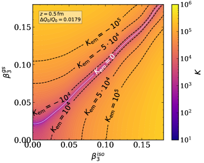
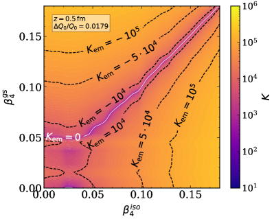
Figure 3: The enhancement factor for new physics searches with ²²⁹$\rm Th$ (“$K$-factor”) as a function of the higher electrostatic multipole moments $\beta_{3}$ (left) and $\beta_{4}$ (right) of the ground state (“gs”) and the isomer (“iso”). We see that $K$ is typically of order $10^{4}$–$10^{5}$, except for a narrow funnel region. In both plots we have fixed $z=0.5\,\rm fm$ and all the other parameters to their median experimental values.

In Fig. 2 we plot the enhancement factor $K$ as a function of the relative quadrupole moment difference between the excited state and the ground state of ²²⁹$\rm Th$, $\Delta Q_{0}/Q_{0}$, for various combinations of $\beta_{3,4}$. We find that the “nightmare scenario” in which $K\simeq 0$, implying no enhanced sensitivity to new physics, is fairly unlikely. It would only be realized for very specific values of $\beta_{3,4}^{\text{gs,iso}}$ of the ground state (“gs”) and the isomer (“iso”) chosen in such a way that the funnel region is aligned with the measured value of $\Delta Q_{0}/Q_{0}$ from Ref. [39] (vertical dark gray line in Fig. 2). In contrast, typical values of $K\sim 10^{4}$–$10^{5}$ are far more likely. To illustrate this point, we plot in Fig. 3 the enhancement factor $K$ as function of $\beta_{3}^{\text{gs}}$ and $\beta_{3}^{\text{iso}}$ for $\beta_{4}^{\text{gs}}=\beta_{4}^{\text{iso}}=0$ (left panel), and as a function of $\beta_{4}^{\text{gs}}$ and $\beta_{4}^{\text{iso}}$ for $\beta_{3}^{\text{gs}}=\beta_{3}^{\text{iso}}=0$ (right panel). In both panels, $\Delta Q_{0}$ has been fixed to the value measured in Ref. [39].

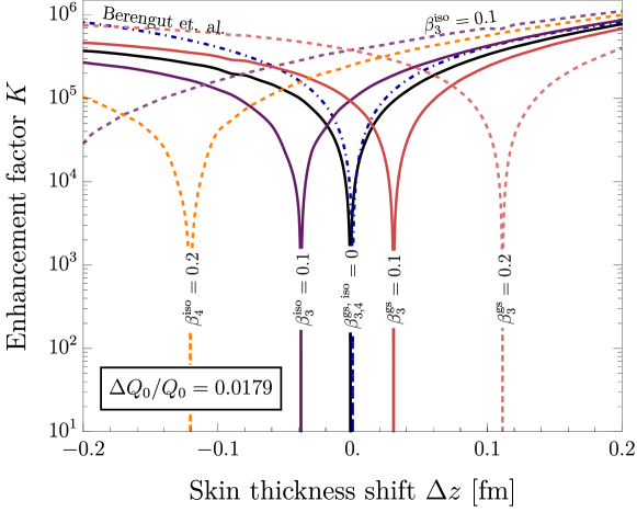
Figure 4: The enhancement factor $K$ as a function of the difference in the skin thickness between the excited and ground states of ²²⁹$\rm Th$. Colored lines correspond to various values of the higher electromagnetic multipole moments $\beta_{3,4}^{\text{gs,iso}}$ of the ground state (“gs”) and the isomer (“iso”), cf. Eq. 8. Similar to Figs. 2 and 3 we see that $K$ can go to zero for specific values of $\Delta z$ and $\beta_{3,4}^{\text{gs, iso}}$, though for most values of these unknown parameters, $K$ is of order $10^{4}$–$10^{5}$. The dot-dashed blue line shows the approximate expression for $K$ from Eq. 7 of Ref. [52], which does not take into account the impact of $\beta_{3,4}$ and is a good approximation only for small $\Delta z$ [59].

We finally discuss in Fig. 4 the impact of the neutron skin thickness, $z$, which we have so far chosen to be $z=$0.5\text{\,}\mathrm{f}\mathrm{m}$$ for both the ground state and the isomer. We see again that – depending on the values of $\Delta z$ and $\beta_{3,4}^{\text{gs,iso}}$ – $K$ might be very small or zero. Note that the treatment of the skin thickness discussed in [52] is valid only for small $\Delta z$ and does not simultaneously take into account the effects of $\beta_{3,4}$.

Finally, We explicitly checked that adding additional contributions to Eq. 11, for instance an exchange term describing Pauli blocking in the free Fermi gas approximation, has a minor effect and does not qualitatively change any of our conclusions. Including such terms would slightly change the values of $\beta_{3,4}^{\text{gs,iso}}$ for which $K\ll 10^{5}$ by a small amount.

2.2 Th-229 as a Halo Nucleus

To describe ²²⁹$\rm Th$ as a halo nucleus, we follow the halo Effective Field Theory (EFT) framework for shallow $d$-wave states developed in [60, 61], considering the ground state ($j=5/2$) and the isomer ($j=3/2$) which both have positive parity as a doublet resulting from the $l=2$ coupling of the halo neutron to the ${{}^{228}\rm Th}$ core system. We stress here that halo EFT should only be considered a model for the neutron–²²⁸$\rm Th$ system, not a proper EFT, as the separation between the low and high energy scales is marginal. If the expansion parameter is estimated as the ratio of the neutron separation energies of ²²⁹$\rm Th$ ($S_{n}\approx$5.2\text{\,}\mathrm{M}\mathrm{e}\mathrm{V}$$) and ²²⁸$\rm Th$ ($S_{n}\approx$7.1\text{\,}\mathrm{M}\mathrm{e}\mathrm{V}$$), it would be $\sqrt{5.2/7.1}\approx 0.86$. In addition, the predictivity of halo EFT is limited for $d$-wave nuclei as the centrifugal barrier creates a strong dependence on short-distance (small $r$) effects and therefore on the overlap of the halo nucleon’s wave function with the core. This is reflected in a leading-order dependence of most observables on counter-terms whose exact magnitude depends on the core–halo interaction model.

However, $d$-wave halo EFT suggests that the neutron-halo doublet states, $j={3/2}$ and $j={5/2}$, are degenerate at leading order, and that therefore the differences between their charge radii, quadrupole moments, etc., vanish at leading order [61, 60]. Thus, we develop here a model, inspired by halo EFT, that focuses on these differences, motivated by the nature of the isomeric transition. We begin by computing the two quantities to which we have experimental access, namely the mean squared charge radius and the quadrupole moment. Within our halo model, the charge density of the ground and excited states are identical, except for a difference stemming from the spin–orbit interaction between the halo neutron’s spin and its $l=2$ orbital angular momentum. This spin–orbit contribution to the charge density is given by [62]

$$\rho_{\text{SO}}=\frac{\mu_{n}}{2m_{n}^{2}}i\sigma_{\alpha\beta}\cdot\Big{[}(\nabla\Phi_{\alpha}^{\dagger})\times(\nabla\Phi_{\beta})\Big{]}\,,$$ (12)

where $\mu_{n}=-1.91$ is the magnetic moment of the neutron in units of the nuclear magneton, $\Phi$ is the (non-relativistic 2-component) neutron spinor and $\alpha,\beta=1,2$ are spinor indices. With $\rho_{\text{SO}}$ at hand we can compute the mean squared charge radius and the quadrupole moment, in analogy to our calculation from Section 2.1 for the geometric model.

We start with the contribution from the spin–orbit charge density to the mean squared radius $\Delta\langle r^{2}\rangle$. Following Ref. [62], it is given by

$$\langle r^{2}\rangle_{\text{SO}}=\frac{1}{Z}\int r^{2}\rho_{\text{SO}}\,d^{3}\mathbf{r}=-\frac{\mu_{n}}{m_{n}^{2}Z}(\kappa+1)\,,$$ (13)

where

$$\kappa=\begin{cases}l&\text{for $j=l-\frac{1}{2}$}\\ -(l+1)&\text{for $j=l+\frac{1}{2}$}\end{cases}\,.$$ (14)

Then, for the difference between the isomer and the ground state we obtain

$$\Delta\langle r^{2}\rangle_{\text{SO}}\equiv\langle r^{2}\rangle_{\text{SO}}^{\text{iso}}-\langle r^{2}\rangle_{\text{SO}}^{\text{gs}}=$0.0047\text{\,}\mathrm{f}\mathrm{m}^{2}$\,.$$ (15)

This value is smaller than the measured $\Delta\langle r^{2}\rangle=$0.012(2)\text{\,}\mathrm{f}\mathrm{m}^{2}$$ [50] by only a factor of $\sim 2$, which we consider excellent agreement given the inherent uncertainties to the halo model.

For the intrinsic nuclear quadrupole moment,

$$Q_{\text{SO}}=\int r^{2}(3\cos^{2}\theta-1)\rho_{\text{SO}}\,d^{3}\mathbf{r}\,,$$ (16)

we find $Q_{\text{SO}}^{\text{gs}}=8\mu_{n}/(5m_{n}^{2})$ for the ground state, and $Q_{\text{SO}}^{\text{gs}}=-3\mu_{n}/(5m_{n}^{2})$ for the isomer. Using again $\mu_{n}=-1.91$ , we find

$$Q_{\text{SO}}^{\text{iso}}-Q_{\text{SO}}^{\text{gs}}=$0.185\text{\,}\mathrm{f}\mathrm{m}^{2}$\,,$$ (17)

in astonishingly good agreement with the latest experimental value [39]

$$(Q^{\text{iso}}-Q^{\text{gs}})_{\text{exp}}=$0.175\,525(6)\text{\,}\mathrm{f}\mathrm{m}^{2}$.$$ (18)

We consider this a further validation of the halo model for ²²⁹$\rm Th$. We also notice that the computations of $\Delta\langle r^{2}\rangle_{\text{SO}}$ and $Q_{\text{SO}}^{\text{iso}}-Q_{\text{SO}}^{\text{gs}}$ are not sensitive to UV physics, i.e., insensitive to the structure of the wave-function near the origin. The main assumption in these calculations is that the contribution originates in single nucleons [62], i.e., consistent with a halo model [54]. This leaves room for possible renormalization of the halo-neutron magnetic moment, which offers an explanation for the $\approx 50\%$ deviation from experiment.

Having shown that the halo model gives sensible results for the mean squared charge radius and the quadrupole moment, we now compute the spin–orbit contribution to the binding energy of the halo neutron [63]

$$E_{\text{SO}}=\frac{e\,\mu_{n}}{2m_{n}^{2}}\frac{1}{2}\bigg{[}j(j+1)-l(l+1)-\frac{3}{4}\bigg{]}\int_{0}^{\infty}\left[\frac{[u(r)]^{2}}{r}\frac{dV_{\rm C}}{dr}\right]dr\,,$$ (19)

where $l=2$ and $j=5/2$ (ground state) or $3/2$ (isomer) are its angular momentum quantum numbers, $V_{\rm C}(r)$ is the Coulomb potential of the ²²⁸$\rm Th$ core, and $u(r)$ is the excess neutron’s radial $d$-wave function [64]:

$$u(r)=A(r)e^{-\gamma r}\Big{(}1+\frac{3}{\gamma r}+\frac{3}{(\gamma r)^{2}}\Big{)}\,.$$ (20)

In this expression, $\gamma\equiv\sqrt{2m_{n}E_{B}}$, $E_{B}=$5.2\text{\,}\mathrm{M}\mathrm{e}\mathrm{V}$$ is the binding energy, and $A(r)$ is determined by short-range physics. $A(r)$ has a weak dependence on $r$, and it asymptotically converges to a constant $A$ at large $r$, that is therefore called the asymptotic normalization constant (ANC). At leading order in halo EFT, $A$ is taken to be fully independent of $r$, and depends on the UV cutoff scale, which is what we assume in the following. As usual in EFTs, the behavior of the ANC at short distances should be fixed from additional experimental constraints, see the discussion in Section 3. Since the neutron separation energy for the ground state of ²²⁹$\rm Th$ is expected to be almost the same as for the isomer, a good assumption is that $u(r)$ is also the same for $j=5/2$ and $j=3/2$. After all, these quantum numbers are just a result of the spin–orbit coupling for fixed $l=2$, and we treat the spin–orbit potential as a small perturbation.

In order to estimate $E_{\text{SO}}$ from Eq. 19, we also need to specify the Coulomb potential, $V_{\rm C}(r)$, which we derive from the nuclear charge density distribution. As the halo-neutron radial wave function is dominated by the length scale $\gamma^{-1}$, i.e., few Fermi, much larger than the UV length-scale, the charge density can be approximated by a Woods–Saxon form [65], see Eq. 6. Since for heavy nuclei $R_{0}\gg z$, we can further approximate the charge density $\rho(r)\approx\frac{3}{4\pi R_{0}^{3}}Ze\,\Theta(R_{0}-r)$, leading to

$$V_{\rm C}(r)=\begin{cases}\frac{Ze}{2R_{0}}\Big{(}3-\big{(}\frac{r}{R_{0}}\big{)}^{2}\Big{)}&\quad r<R_{0}\\ \frac{Ze}{r}&\quad r>R_{0}\end{cases}\,.$$ (21)

Thus, the universal property $\rho\approx\text{constant}$ leads to $dV_{\rm C}/dr\propto r$, which conveniently cancels the UV sensitivity of the integral in Eq. 19, i.e.,

$$\int_{0}^{\infty}\frac{[u(r)]^{2}}{r}\frac{dV_{\rm C}}{dr}dr=\frac{Ze}{R_{0}}\left(\frac{1}{R_{0}^{2}}\int_{0}^{R_{0}}[u(r)]^{2}dr+\int_{R_{0}}^{\infty}R_{0}[u(r)]^{2}\frac{dr}{r^{3}}\right)\,.$$ (22)

Thus, $\int_{0}^{\infty}\frac{(u(r))^{2}}{r}\frac{dV_{\rm C}}{dr}dr$ is not divergent. Both integrals on the right-hand side are finite, the first one due to the normalization of $u(r)$, and the second because it is controlled by the free $d$-wave solution, cf. Eq. 20. For the parameters of ²²⁹$\rm Th$, the first integral dominates. In order to evaluate this integral we introduce a short-distance cutoff, $l$, to regularize the divergence of the integrand at $r\to 0$, and we assume a constant $A(r)$, constrained by the normalization condition on $u(r)$. We find that the integral is almost independent of $l$ for values $l\leq$4\text{\,}\mathrm{f}\mathrm{m}$$. Numerically, we then obtain

$$\Delta E_{\text{SO}}=\left.E_{\text{SO}}\right\rvert_{j=5/2}-E_{\text{SO}}|_{j=3/2}\approx 144\,p\,\text{keV}\,,$$ (23)

where the order-one factor $p$ is a function of $A$ and $l$. A more complete nuclear model would predict a specific form for $A(r)$, eliminating the need for a regulator, and thereby determining $p$. Intuitively, $p$ is related to the probability of finding the halo neutron inside the nucleus.

Summarizing, we find the contribution of the spin–orbit interaction to $\Delta E_{\text{em}}$ to be of order $100\text{\,}\mathrm{k}\mathrm{e}\mathrm{V}$, which corresponds to an enhancement factor $K\approx 10^{4}$ for new physics searches using nuclear clocks.

3 Summary and Outlook

In this work we have studied how the sensitivity of a ²²⁹$\rm Th$ nuclear clock to new physics depends on nuclear modelling. On the one hand, we have shown that within a classical geometric model of the ²²⁹$\rm Th$ nucleus, which is widely used in the literature, a “nightmare scenario” in which the sensitivity goes to zero is possible, although it requires fine-tuning of the model parameters at the per cent or per mille level. On the other hand, we have presented a more realistic quantum halo model, in which an approximately unpaired neutron of ²²⁹$\rm Th$ is loosely bound to a ²²⁸$\rm Th$ spin-0 core. The neutron is in a $d$-wave state, with orbital angular momentum $l=2$. We have validated this model against the experimentally measured differences of charge radii and quadrupole moments of the ²²⁹$\rm Th$ ground state and of the isomer ${}^{229\text{m}}$$\rm Th$. The model correctly predicts these differences to be close to zero. Within the halo model, the “nightmare scenario” is never realized and the enhancement factor $K_{\text{em}}$ for new physics searches is always $\gtrsim 10^{4}$.

Our work suggests multiple directions of future research. It is clear that the main obstacle to an accurate determination of the enhancement factor is the nuclear model, which has multiple unknown parameters. In the future, we hope it will be possible to further refine and verify the halo model using in particular neutron capture experiments. The amplitude of neutron capture in $d$–wave halos is proportional to the asymptotic normalization constant $A$. Thus, a neutron capture experiment can give a quantitative constraint on the probability of finding the halo-neutron inside the core, which governs the size of the spin–orbit contribution to the electromagnetic interaction. In addition, we have assumed that $A$ is identical for the ground state and for the isomer. This assumption can, in principle, be verified by measuring the neutron capture cross section, $\sigma_{\text{cap}}$, for both states. Halo EFT predicts $\sigma_{\text{cap}}^{\text{iso}}=\frac{2}{3}\sigma_{\text{cap}}^{\text{gs}}$ [60].

Moreover, it is important to confirm the latest results for $\Delta Q_{0}/Q_{0}$ [39], and to possibly also improve the determination of $\Delta\langle r^{2}\rangle$. In addition, it is highly desirable to devise further tests of the shape of the nucleus, sensitive to the higher-order multipoles $\beta_{3,4}$ and the skin thickness $z$. These quantities are crucial for determining the enhancement factor within the classical geometric model, which – despite the shortcomings we have stressed several times – is still of interest and represents an alternative to the $d$–wave halo model.

Finally, we have argued in the introduction to Section 2 that $K_{\text{em}}\sim K_{s}$, and that therefore our results apply both to new physics coupled to the electromagnetic sector and to new physics coupled to the strong sector. We believe this to be true unless the electromagnetic and nuclear energy differences between the ground and excited states of thorium-229 conspire to have the exact same functional dependence on $\alpha_{s}$. Indeed, in EFT approaches to the expansion of nuclear forces in the QCD scale, the electromagnetic and strong contributions are predicted to have different dependence on this scale [66, 55]. However, it is key to verify this within concrete frameworks. We leave this and other exciting developments for future work.

Appendix A Spin-Orbit Contribution to the quadrupole moment

Here we provide details on the computation of the spin–orbit contribution to the intrinsic nuclear quadrupole moment for halo nuclei. In general, this contribution is

$$Q_{\text{SO}}=\int r^{2}(3\cos^{2}\theta-1)\rho_{\text{SO}}\,d^{3}\mathbf{r}.$$ (24)

Following the appendix of ref. [62], we split $Q_{\text{SO}}$ into two pieces. The first one is

$$Q_{\text{SO}}^{(1)}=-\frac{3\mu_{n}}{2m_{n}^{2}}\left(\kappa+1\right)\int\!d\cos\theta\,d\phi\,\Omega^{\dagger}_{jlm}\Omega_{jlm}\,(3\cos^{2}\theta-1),$$ (25)

where

$$\Omega_{jlm}=\begin{pmatrix}C_{lm-\frac{1}{2},\frac{1}{2}\frac{1}{2}}^{jm}Y_{l}^{m-\frac{1}{2}}\\ C_{lm+\frac{1}{2},\frac{1}{2}-\frac{1}{2}}^{jm}Y_{l}^{m+\frac{1}{2}}\end{pmatrix}$$ (26)

is the angular part of the spinor, and the $C$ are Clebsch–Gordan coefficients relating the orbital angular momentum $l$ and the spin to the total angular momentum $j$. In our case, $l=2$, $j=5/2$ (ground state) or $3/2$ (isomer), and the choice of $m$ is arbitrary as the corresponding phase factors drop out in $\Omega^{\dagger}_{jlm}\Omega_{jlm}$.

The second contribution to $Q_{\text{SO}}$ is more involved and reads [62]

$$Q_{\text{\rm SO}}^{(2)} =\frac{\mu_{n}}{2m_{n}^{2}}\int\!d\theta\,d\phi\,i\bigg{[}\cos\theta\bigg{(}\frac{\partial\Omega_{1}^{\dagger}}{\partial\theta}\frac{\partial\Omega_{1}}{\partial\phi}-\frac{\partial\Omega_{1}^{\dagger}}{\partial\phi}\frac{\partial\Omega_{1}}{\partial\theta}\bigg{)}$$

$$\hskip 51.21504pt+\sin\theta e^{-i\phi}\bigg{(}\frac{\partial\Omega_{1}^{\dagger}}{\partial\theta}\frac{\partial\Omega_{2}}{\partial\phi}-\frac{\partial\Omega_{1}^{\dagger}}{\partial\phi}\frac{\partial\Omega_{2}}{\partial\theta}\bigg{)}$$

$$\hskip 51.21504pt+\sin\theta e^{i\phi}\bigg{(}\frac{\partial\Omega_{2}^{\dagger}}{\partial\theta}\frac{\partial\Omega_{1}}{\partial\phi}-\frac{\partial\Omega_{2}^{\dagger}}{\partial\phi}\frac{\partial\Omega_{1}}{\partial\theta}\bigg{)}$$

$$\hskip 51.21504pt-\cos\theta\bigg{(}\frac{\partial\Omega_{2}^{\dagger}}{\partial\theta}\frac{\partial\Omega_{2}}{\partial\phi}-\frac{\partial\Omega_{2}^{\dagger}}{\partial\phi}\frac{\partial\Omega_{2}}{\partial\theta}\bigg{)}\bigg{]}(3\cos^{2}\theta-1).$$ (27)

Here, we have omitted the indices $jlm$ on $\Omega_{jlm}$ to shorten the notation. The subscripts $1$, $2$ refer to the two components of the spinor. The integrals in Eqs. 25 and 27 can be performed analytically, and the total spin–orbit contribution to the quadrupole moment,

$$Q_{\text{SO}}=Q_{\text{SO}}^{(1)}+Q_{\text{SO}}^{(2)}$$ (28)

is found to be $Q_{\text{SO}}^{\text{gs}}=8\mu_{n}/(5m_{n}^{2})$ for the ground state, and $Q_{\text{SO}}^{\text{gs}}=-3\mu_{n}/(5m_{n}^{2})$ for the isomer, as written in the main text.

References

- [1] J. Preskill, M. B. Wise, and F. Wilczek, Cosmology of the Invisible Axion, Phys. Lett. B 120 (1983) 127–132.
- [2] L. F. Abbott and P. Sikivie, A Cosmological Bound on the Invisible Axion, Phys. Lett. B 120 (1983) 133–136.
- [3] M. Dine and W. Fischler, The Not So Harmless Axion, Phys. Lett. B 120 (1983) 137–141.
- [4] A. Hook, TASI Lectures on the Strong CP Problem and Axions, PoS TASI2018 (2019) 004, [1812.02669].
- [5] L. Di Luzio, M. Giannotti, E. Nardi, and L. Visinelli, The landscape of QCD axion models, Phys. Rept. 870 (2020) 1–117, [2003.01100].
- [6] A. Arvanitaki, J. Huang, and K. Van Tilburg, Searching for dilaton dark matter with atomic clocks, Phys. Rev. D 91 (2015), no. 1 015015, [1405.2925].
- [7] J. Hubisz, S. Ironi, G. Perez, and R. Rosenfeld, A note on the quality of dilatonic ultralight dark matter, Phys. Lett. B 851 (2024) 138583, [2401.08737].
- [8] A. Banerjee, H. Kim, and G. Perez, Coherent relaxion dark matter, Phys. Rev. D 100 (2019), no. 11 115026, [1810.01889].
- [9] A. Chatrchyan and G. Servant, Relaxion dark matter from stochastic misalignment, JCAP 06 (2023) 036, [2211.15694].
- [10] F. Piazza and M. Pospelov, Sub-eV scalar dark matter through the super-renormalizable Higgs portal, Phys. Rev. D 82 (2010) 043533, [1003.2313].
- [11] M. Dine, G. Perez, W. Ratzinger, and I. Savoray, Nelson–Barr ultralight dark matter, 2405.06744.
- [12] V. V. Flambaum and A. F. Tedesco, Dependence of nuclear magnetic moments on quark masses and limits on temporal variation of fundamental constants from atomic clock experiments, Phys. Rev. C 73 (2006) 055501, [nucl-th/0601050].
- [13] T. Damour and J. F. Donoghue, Phenomenology of the Equivalence Principle with Light Scalars, Class. Quant. Grav. 27 (2010) 202001, [1007.2790].
- [14] T. Damour and J. F. Donoghue, Equivalence Principle Violations and Couplings of a Light Dilaton, Phys. Rev. D 82 (2010) 084033, [1007.2792].
- [15] D. Antypas et al., New Horizons: Scalar and Vector Ultralight Dark Matter, 2203.14915.
- [16] H. Kim and G. Perez, Oscillations of atomic energy levels induced by QCD axion dark matter, Phys. Rev. D 109 (2024), no. 1 015005, [2205.12988].
- [17] A. Hook and J. Huang, Probing axions with neutron star inspirals and other stellar processes, JHEP 06 (2018) 036, [1708.08464].
- [18] R. Balkin, J. Serra, K. Springmann, S. Stelzl, and A. Weiler, White dwarfs as a probe of exceptionally light QCD axions, Phys. Rev. D 109 (2024), no. 9 095032, [2211.02661].
- [19] A. Banerjee, G. Perez, M. Safronova, I. Savoray, and A. Shalit, The phenomenology of quadratically coupled ultra light dark matter, JHEP 10 (2023) 042, [2211.05174].
- [20] Y. V. Stadnik and V. V. Flambaum, Can dark matter induce cosmological evolution of the fundamental constants of Nature?, Phys. Rev. Lett. 115 (2015), no. 20 201301, [1503.08540].
- [21] A. Hees, J. Guéna, M. Abgrall, S. Bize, and P. Wolf, Searching for an oscillating massive scalar field as a dark matter candidate using atomic hyperfine frequency comparisons, Phys. Rev. Lett. 117 (2016), no. 6 061301, [1604.08514].
- [22] C. J. Kennedy, E. Oelker, J. M. Robinson, T. Bothwell, D. Kedar, W. R. Milner, G. E. Marti, A. Derevianko, and J. Ye, Precision Metrology Meets Cosmology: Improved Constraints on Ultralight Dark Matter from Atom-Cavity Frequency Comparisons, Phys. Rev. Lett. 125 (2020), no. 20 201302, [2008.08773].
- [23] W. M. Campbell, B. T. McAllister, M. Goryachev, E. N. Ivanov, and M. E. Tobar, Searching for Scalar Dark Matter via Coupling to Fundamental Constants with Photonic, Atomic and Mechanical Oscillators, Phys. Rev. Lett. 126 (2021), no. 7 071301, [2010.08107].
- [24] T. Kobayashi et al., Search for Ultralight Dark Matter from Long-Term Frequency Comparisons of Optical and Microwave Atomic Clocks, Phys. Rev. Lett. 129 (2022), no. 24 241301, [2212.05721].
- [25] X. Zhang, A. Banerjee, M. Leyser, G. Perez, S. Schiller, D. Budker, and D. Antypas, Search for Ultralight Dark Matter with Spectroscopy of Radio-Frequency Atomic Transitions, Phys. Rev. Lett. 130 (2023), no. 25 251002, [2212.04413].
- [26] N. Sherrill et al., Analysis of atomic-clock data to constrain variations of fundamental constants, New J. Phys. 25 (2023), no. 9 093012, [2302.04565].
- [27] A. Banerjee, D. Budker, M. Filzinger, N. Huntemann, G. Paz, G. Perez, S. Porsev, and M. Safronova, Oscillating nuclear charge radii as sensors for ultralight dark matter, 2301.10784.
- [28] I. Kozyryev, Z. Lasner, and J. M. Doyle, Enhanced sensitivity to ultralight bosonic dark matter in the spectra of the linear radical SrOH, Phys. Rev. A 103 (2021), no. 4 043313, [1805.08185].
- [29] E. Madge, G. Perez, and Z. Meir, Prospects of nuclear-coupled-dark-matter detection via correlation spectroscopy of I2+ and Ca+, Phys. Rev. D 110 (2024), no. 1 015008, [2404.00616].
- [30] R. Oswald et al., Search for Dark-Matter-Induced Oscillations of Fundamental Constants Using Molecular Spectroscopy, Phys. Rev. Lett. 129 (2022), no. 3 031302, [2111.06883].
- [31] E. Peik and C. Tamm, Nuclear laser spectroscopy of the 3.5 eV transition in Th-229, EPL (Europhysics Letters) 61 (Jan., 2003) 181–186.
- [32] C. J. Campbell, A. G. Radnaev, A. Kuzmich, V. A. Dzuba, V. V. Flambaum, and A. Derevianko, Single-Ion Nuclear Clock for Metrology at the 19th Decimal Place, Phys. Rev. Lett. 108 (Mar., 2012) 120802, [1110.2490].
- [33] G. A. Kazakov, A. N. Litvinov, V. I. Romanenko, L. P. Yatsenko, A. V. Romanenko, M. Schreitl, G. Winkler, and T. Schumm, Performance of a 229Thorium solid-state nuclear clock, New Journal of Physics 14 (Aug., 2012) 083019, [1204.3268].
- [34] L. von der Wense and B. Seiferle, The 229Th isomer: prospects for a nuclear optical clock, Eur. Phys. J. A 56 (2020), no. 11 277, [2009.13633].
- [35] S. Kraemer et al., Observation of the radiative decay of the 229Th nuclear clock isomer, Nature 617 (2023), no. 7962 706–710, [2209.10276].
- [36] P. G. Thirolf, S. Kraemer, D. Moritz, and K. Scharl, The thorium isomer 229mTh: review of status and perspectives after more than 50 years of research, European Physical Journal Special Topics (Jan., 2024).
- [37] J. Tiedau et al., Laser Excitation of the Th-229 Nucleus, Phys. Rev. Lett. 132 (2024), no. 18 182501.
- [38] R. Elwell, C. Schneider, J. Jeet, J. E. S. Terhune, H. W. T. Morgan, A. N. Alexandrova, H. B. Tran Tan, A. Derevianko, and E. R. Hudson, Laser Excitation of the Th229 Nuclear Isomeric Transition in a Solid-State Host, Phys. Rev. Lett. 133 (2024), no. 1 013201, [2404.12311].
- [39] C. Zhang et al., Dawn of a nuclear clock: frequency ratio of the 229mTh isomeric transition and the 87Sr atomic clock, 2406.18719.
- [40] E. Fuchs, F. Kirk, E. Madge, C. Paranjape, E. Peik, G. Perez, W. Ratzinger, and J. Tiedau To appear, 2024.
- [41] V. V. Flambaum, Enhanced effect of temporal variation of the fine structure constant and the strong interaction in Th-229, Phys. Rev. Lett. 97 (2006) 092502, [physics/0604188].
- [42] P. Fadeev, J. C. Berengut, and V. V. Flambaum, Sensitivity of 229Th nuclear clock transition to variation of the fine-structure constant, Phys. Rev. A 102 (2020), no. 5 052833, [2007.00408].
- [43] W. G. Rellergert, D. DeMille, R. R. Greco, M. P. Hehlen, J. R. Torgerson, and E. R. Hudson, Constraining the Evolution of the Fundamental Constants with a Solid-State Optical Frequency Reference Based on the Th-229 Nucleus, Phys. Rev. Lett. 104 (2010) 200802.
- [44] M. S. Safronova, The Search for Variation of Fundamental Constants with Clocks, Annalen Phys. 531 (2019), no. 5 1800364.
- [45] E. Peik, T. Schumm, M. S. Safronova, A. Pálffy, J. Weitenberg, and P. G. Thirolf, Nuclear clocks for testing fundamental physics, Quantum Sci. Technol. 6 (2021), no. 3 034002, [2012.09304].
- [46] A. C. Hayes, J. L. Friar, and P. Möller, Splitting sensitivity of the ground and 7.6 ev isomeric states of , Phys. Rev. C 78 (Aug, 2008) 024311.
- [47] H. Banks, E. Fuchs, and M. McCullough, A Nuclear Interferometer for Ultra-Light Dark Matter Detection, 2407.11112.
- [48] B. Maheshwari and A. K. Jain, Nuclear isomers at the extremes of their properties, Eur. Phys. J. ST 233 (2024), no. 5 1101–1111, [2402.03976].
- [49] P. G. Thirolf, S. Kraemer, D. Moritz, and K. Scharl, The thorium isomer 229mTh: review of status and perspectives after more than 50 years of research, Eur. Phys. J. ST 233 (2024), no. 5 1113–1131.
- [50] J. Thielking, M. V. Okhapkin, P. Głowacki, D. M. Meier, L. von der Wense, B. Seiferle, C. E. Düllmann, P. G. Thirolf, and E. Peik, Laser spectroscopic characterization of the nuclear-clock isomer229mTh, Nature 556 (2018), no. 7701 321–325, [1709.05325].
- [51] M. S. Safronova, S. G. Porsev, M. G. Kozlov, J. Thielking, M. V. Okhapkin, P. Głowacki, D. M. Meier, and E. Peik, Nuclear charge radii of 229Th from isotope and isomer shifts, Phys. Rev. Lett. 121 (2018), no. 21 213001, [1806.03525].
- [52] J. C. Berengut, V. A. Dzuba, V. V. Flambaum, and S. G. Porsev, A Proposed experimental method to determine alpha-sensitivity of splitting between ground and 7.6-eV isomeric states in Th-229, Phys. Rev. Lett. 102 (2009) 210801, [0903.1891].
- [53] T. Naito, X. Roca-Maza, G. Colò, and H. Liang, Effects of finite nucleon size, vacuum polarization, and electromagnetic spin-orbit interaction on nuclear binding energies and radii in spherical nuclei, Phys. Rev. C 101 (2020), no. 6 064311, [2003.03177].
- [54] H. W. Hammer, C. Ji, and D. R. Phillips, Effective field theory description of halo nuclei, J. Phys. G 44 (2017), no. 10 103002, [1702.08605].
- [55] H. W. Hammer, S. König, and U. van Kolck, Nuclear effective field theory: status and perspectives, Rev. Mod. Phys. 92 (2020), no. 2 025004, [1906.12122].
- [56] E. Browne and J. K. Tuli, Nuclear Data Sheets for A = 229, Nucl. Data Sheets 109 (2008) 2657–2724.
- [57] K. Abusaleem, Nuclear Data Sheets for A=228, Nucl. Data Sheets 116 (2014) 163–262.
- [58] R. D. Woods and D. S. Saxon, Diffuse surface optical model for nucleon-nuclei scattering, Phys. Rev. 95 (Jul, 1954) 577–578.
- [59] H. De Vries, C. De Jager, and C. De Vries, Nuclear charge-density-distribution parameters from elastic electron scattering, Atomic Data and Nuclear Data Tables 36 (1987), no. 3 495–536.
- [60] J. Braun, H.-W. Hammer, and L. Platter, Halo structure of 17C, Eur. Phys. J. A 54 (2018), no. 11 196, [1806.01112].
- [61] J. Braun, W. Elkamhawy, R. Roth, and H. W. Hammer, Electric structure of shallow D-wave states in Halo EFT, J. Phys. G 46 (2019), no. 11 115101, [1803.02169].
- [62] A. Ong, J. C. Berengut, and V. V. Flambaum, The Effect of spin-orbit nuclear charge density corrections due to the anomalous magnetic moment on halonuclei, Phys. Rev. C 82 (2010) 014320, [1006.5508].
- [63] J. J. Sakurai, Modern Quantum Mechanics (2nd Edition). Addison Wesley, January, 1994.
- [64] V. Zelevinsky and A. Volya, Physics of Atomic Nuclei. Wiley-VCH, 2017.
- [65] W. N. Cottingham and D. A. Greenwood, An Introduction to Nuclear Physics. Cambridge University Press, 2001.
- [66] U.-G. Meißner, Anthropic considerations in nuclear physics, Sci. Bull. 60 (2015), no. 1 43–54, [1409.2959].