Phase transitions in $q$-state clock model

Abstract

The $q-$state clock model, sometimes called the discrete $XY$ model, shows interesting critical phenomena. While $q=2$ corresponds to the Ising model, the $q\to\infty$ limit corresponds to the well-known $XY$ model. It is known that up to $q=4$, the two-dimensional (2D) clock model exhibits a second-order (symmetry-breaking) phase transition. On the other hand, the 2D $XY$ model only shows a topological (Berezinskii-Kosterlitz-Thouless or BKT) phase transition. Interestingly, the model with finite $q$ (with $q\geq 5$) is predicted to show two different phase transitions. There are varying opinions about the actual characters of the transitions, especially the one at the lower temperature. In this work we develop mean-field theory (basic and higher order) to study the $q$-state clock model systematically. Using the mean-field theory, we show that the phase transition at the higher temperature is of the BKT type. We find that this transition temperature ($T_{BKT}$) does not depend on the $q$ values, and our basic (zeroth order) mean-field calculation shows that $T_{BKT}=2J/k_{B}$, where $J$ is the nearest-neighbor exchange constant and $k_{B}$ is the Boltzmann constant. Our analysis shows that the other phase transition is a spontaneous symmetry-breaking (SSB) type. The corresponding transition temperature ($T_{SSB}$) is found to decrease with increasing $q$ value; it is found that $T_{SSB}\propto 1/q^{2}$ with a weak logarithmic correction. To better understand the model, we also perform the first-order mean-field calculations (here, the interaction between two targeted nearest neighbors is treated exactly). This calculation gives us $T_{BKT}=1.895J/k_{B}$, which is slightly closer to the reported value of $0.893J/k_{B}$. The main advantage of this higher-order mean-field theory is that one can now estimate the spin-spin correlation, whose change in the properties indicates the phase transition.

I Introduction

The $q-$state clock model, a variant of the Potts model [1, 2], represents the Ising model and the $XY$ model in two different limits of $q$; the clock model becomes the Ising model when $q=2$ and it becomes the $XY$ model in the $q\to\infty$ limit [3, 4, 5]. These two models in two-dimension show two different types of phase transitions [6, 7]. The two-dimensional (2D) Ising model shows a second-order (spontaneous symmetry-breaking) phase transition [8]. On the other hand, the 2D $XY$ model does not show the spontaneous symmetry-breaking phase transition (by the Wagner-Mermin theorem [9]), it still shows a topological (bound vortex-antivortex to unbound vortex and antivortex) transition, known as Berezinskii-Kosterlitz-Thouless or BKT transition [10, 11, 12, 13].

The $q-$state clock model, without magnetic field, is represented by the following Hamiltonian:

$$H=-J\sum_{\langle ij\rangle}{\cos{(\theta_{i}-\theta_{j})}},$$ (1)

where $J$ is the nearest-neighbor exchange constant and $\langle{ij}\rangle$ represents summation over the nearest neighbors. Here $\theta_{i}$ is the angle between the $i$-th spin and the reference, say $X$, axis. This angle takes $q$ possible values $\theta_{i}=2\pi k_{i}/q$ where $k_{i}$ can take any integer value from 1 to $q$. Since the Ising and the $XY$ model show two different types of phase transitions, it is interesting to ask what happens to the 2D clock model when $q$ is finite and $q>2$. It is known that for $q\leq 4$, the 2D clock model shows only one phase transition, which is of the spontaneous symmetry-breaking type [5, 14]. For $q\geq 5$, this model is known to show two phase transitions [3, 4, 5, 14]. There are opposite views on the nature of these phase transitions. Although it is mostly accepted that the transition at the higher temperature is of BKT type, some authors argued that the transition at the lower temperature corresponds to the spontaneous symmetry-breaking type [4, 15, 14], while some other authors argued that the transition is of BKT type [5]. To better understand the nature of the transitions and gain deeper insight into the different properties of the model, we develop a mean-field theory for the $q-$state clock model. To the best of our knowledge, ours is the first systematic mean-field study of the $q$-state clock model.

The mean-field theory is an important approach to analyze properties of model systems [6]. Its success in analyzing classical or quantum models is well known. The mean-field theories work better in the higher dimensions and/ or when the coordination number is large. Although, in this work, we are mainly interested in the two-dimensional systems, we expect to get reasonable results in the large $q$ limit. This is because the change in the mean-field will be much less due to elementary excitation or low-temperature fluctuation in the neighbors. We study two phase transitions at large $q$ using our mean-field approach. We find that the transition at the higher temperature is $q$ independent and is of the BKT type, while the transition at the lower temperature changes as $1/q^{2}$ and is of the spontaneous symmetry-breaking type. To better understand the physics of the 2D clock model, we also developed a higher-order mean-field theory and estimated the spin-spin correlation using the theory, besides making an improved estimation of the BKT transition temperature.

This article is arranged in the following way. In Sec. II, we develop the zeroth order mean-field theory for the 2D clock model for a generic value of $q$. Next, in Sec. III, we construct the first order mean-field theory. Using this higher order theory, we estimate the nearest-neighbor spin-spin correlation and find a better estimation of the BKT transition temperature. We conclude our work in Sec. IV.

II Mean-Field Theory

The $q-$state clock model represents a spin system where the spins lie in the $XY$ plane and can orient only in $q$ possible directions. Eq. 1 gives the Hamiltonian corresponding to this model. As the exact results for this model are scarce, it is important to develop an appropriate mean-field approach to understand the behavior of this model.

To go further, we first define a complex spin variable $S_{k}$ corresponding to the $k$-th spin: $S_{k}=e^{i\theta_{k}}$, where $\theta_{k}=2\pi j_{k}/q$. Here $j_{k}$ takes any value from 1 to $q$. With this complex spin variable, we can rewrite the Hamiltonian in Eq. 1 as,

$$H=-JRe{\sum{S_{i}S^{*}_{j}}}.$$ (2)

We now perform the basic (zero-th order) mean-field theory over the complex spin variables. In the mean-field approach, each variable ($S_{i}$) is replaced by its mean value plus a small fluctuation term ($\delta S_{i}$),

$$S_{i}=\langle S_{i}\rangle+\delta S_{i}.$$

If we define the complex mean-field parameter as $l=\sum_{i=1}^{N}{\frac{\langle S_{i}\rangle}{N}}$, for translationally invarient system, we can write

$$S_{i}S^{*}_{j}=(l+\delta S_{i})(l+\delta S_{j})^{*}\approx|l|^{2}+l\delta S_{j}^{*}+l^{*}\delta S_{i},$$

after neglecting the small term $\delta S_{i}\delta S^{*}_{j}$. After replacing $\delta S_{i}$ by $S_{i}-l$, we get the following mean-field Hamiltonian from Eq. 2,

$$H_{MF}=-JRe{\sum_{\langle ij\rangle}{(|l|^{2}+l^{*}(S_{i}-l)+l(S_{j}-l)^{*})}}.$$ (3)

We here note that $\sum_{\langle ij\rangle}S_{i}=\sum_{\langle ij\rangle}S_{j}$ and $\sum_{\langle ij\rangle}=\frac{1}{2}\sum_{i=1}^{N}\sum_{j\in(nn)}$, where $\sum_{j\in(nn)}$ represents the sum over the nearest neighbors, $N$ is the total number of lattice sites. With these, we get

$$H_{MF}=-J\frac{1}{2}Re(-{{Nr{|l|}^{2}+r\sum_{i=1}^{N}(l^{*}S_{i}+lS^{*}_{i}))}},$$ (4)

where $r$ is the number of nearest neighbors. As $l^{*}S_{i}+lS^{*}_{i}=2Re(l^{*}S_{i})$, we can write

$$H_{MF}=\frac{1}{2}{{NJr{|l|}^{2}-Jr\sum_{i=1}^{N}Re(l^{*}S_{i})}}.$$ (5)

The mean-field parameter $l$ is a complex quantity, which we now write in terms of two real parameters: $l=l_{1}+il_{2}$. Physically, $l_{1}$ and $l_{2}$ represent the average values of the $X$ and the $Y$ components of a spin. With $S_{j}=\cos{\frac{2\pi j_{k}}{q}}+i\sin{\frac{2\pi j_{k}}{q}}$, we can recast Eq. 5 as

$$H_{MF}=\frac{1}{2}NJr(l_{1}^{2}+l_{2}^{2})-Jr\sum_{i=1}^{N}(l_{1}\cos{\frac{2\pi i_{k}}{q}}+l_{2}\sin{\frac{2\pi i_{k}}{q}}).$$ (6)

It may be mentioned again here that $i_{k}$ can take any of the $q$ values from 1 to $q$. If we write $H_{MF}=\sum_{i}^{N}h_{i}$, we get the following effective mean-field Hamiltonian corresponding to the $i-$th site,

$$h_{i}=\frac{1}{2}Jr(l_{1}^{2}+l_{2}^{2})-Jr(l_{1}\cos{\frac{2\pi i_{k}}{q}}+l_{2}\sin{\frac{2\pi i_{k}}{q}}).$$ (7)

The $q$ possible values of $h_{i}$ are given by

$$\epsilon(k)=\frac{1}{2}Jr(l_{1}^{2}+l_{2}^{2})-r(l_{1}\cos{\frac{2\pi k}{q}}+l_{2}\sin{\frac{2\pi k}{q}}),$$ (8)

where $k$ takes any value between 1 and $q$. The energy $\epsilon(k)$ does not depend on the site index $i$ for a transitionally invariant system.

In the following, we will calculate the free energy to determine $l_{1}$ and $l_{2}$ and to analyze the equilibrium properties from the free energy minima at a given temperature.

The partition function of each spin is given by,

$$z_{i}=\sum_{k=1}^{q}e^{-\beta\epsilon(k)}$$ (9)

Since the spins in the mean-field approach are non-interacting, the total partition function of the system is given by $Z={z_{i}}^{N}$. The free energy corresponding to a single spin is

$$F=-\frac{\ln{z_{i}}}{\beta},$$ (10)

where $\beta=\frac{1}{k_{B}T}$ with $k_{B}$ being the Boltzmann constant and $T$ being the absolute temperature. Written explicitly, we get

$$F=\frac{Jr(l^{2}_{1}+l^{2}_{2})}{2}-\frac{1}{\beta}\ln\sum_{k=1}^{q}e^{\beta Jr(l_{1}\cos{\frac{2\pi k}{q}}+l_{2}\sin{\frac{2\pi k}{q}})}.$$ (11)

II.1 Free energy plots at different temperatures

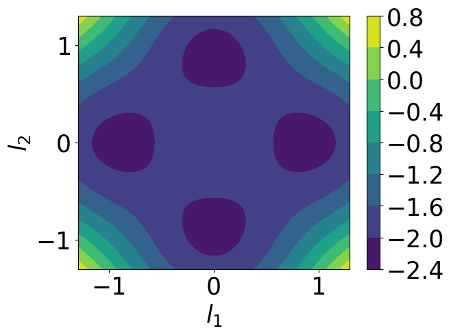
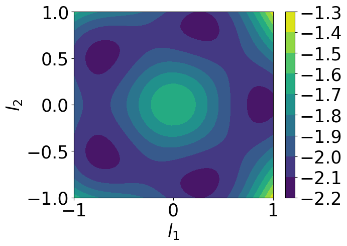
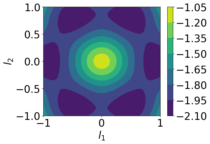
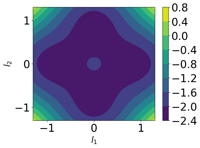
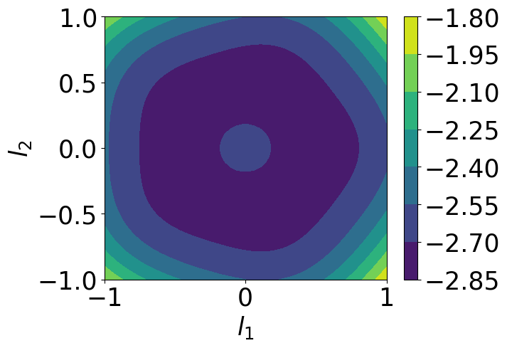
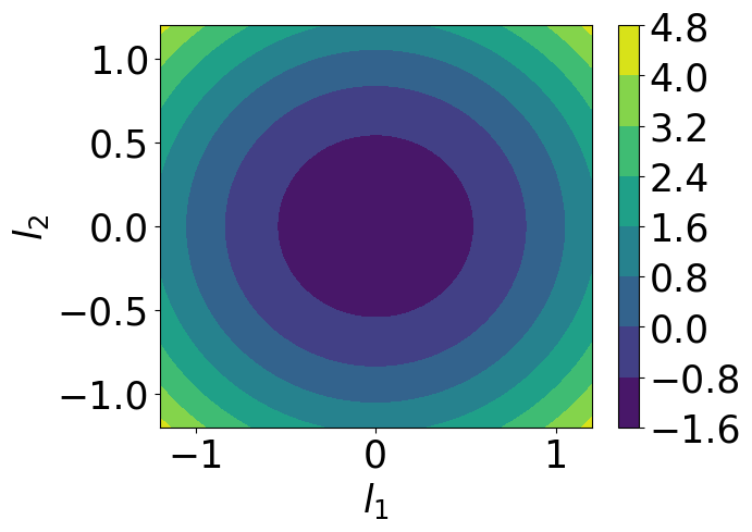
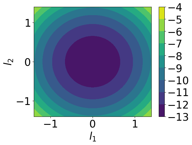
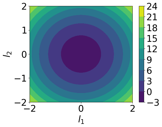
 a)                                           b)                                             c)                                              a)                                          b)                                              c)                                              a)                                             b)                                          c)                                      

Figure 1: Free energy at low-temperature: 3 $q=4$, 3 $q=5$, 3 $q=6$.

Figure 2: Free energy at intermediate-temperature: 3 $q=4$, 3 $q=5$, 3 $q=6$.

Figure 3: Free energy at high-temperature: 3 $q=4$, 3 $q=5$, 3 $q=6$.

The free energy $F$ in Eq. 11 is a function of $l_{1}$, $l_{2}$ and $\beta$. The system equilibrium for a given temperature corresponds to the free energy minimum (minima) with respect to $l_{1}$ and $l_{2}$. Thus, to first gain insight into the problem, we plot $F$ as a function of $l_{1}$ and $l_{2}$ for different fixed temperatures. The plots can be seen in Figs. 3,3 and 3. First, we note that, at high temperatures, we have only one minimum at $l_{1}=l_{2}=0$ (Fig. 3). On the other hand, at low temperatures, we have a local maximum at the origin ($l_{1}=l_{2}=0$) but $q$ number of minima around the origin (Fig. 3). Interestingly, there is an intermediate range of temperature where we get a ring of minima around the origin (Fig. 3).

Noting again that the parameters $l_{1}$ and $l_{2}$ respectively represent the average values of the $X$ and $Y$ components of a spin, we can have the following interpretations of the above observations. At high temperatures, we have one free energy minimum at the origin. This corresponds to the disordered (paramagnetic) phase. In this phase, an individual spin can orient along any possible direction ($|l|^{2}=l_{1}^{2}+l_{2}^{2}=0$). As we lower the temperature, we see the minimum turns into a local maximum, and a ring of minima forms around the maxima. Unlike in the paramagnetic phase, in this new phase, individual spins orient in a fixed direction ($|l|^{2}=l_{1}^{2}+l_{2}^{2}\neq 0$), but different spins orient in different directions. We identify this phase with the vortex-antivortex bound or Berezinskii-Kosterlitz-Thouless (BKT) phase. The transition between the paramagnetic phase and the BKT phase can be called the BKT phase transition, and the corresponding temperature may be denoted by $T_{BKT}$. It may be noted here that the spin symmetry is not broken due to this BKT transition; if we choose a spin randomly, it may be found to be oriented along any of the $q$ possible directions in both phases.

Starting from the BKT phase, if we lower the temperature further, the ring of minima will slowly disappear, and $q$ distinct localized minima will form (Fig. 3). Although all $q$ minima are equally probable for a spin to be found, the system will spontaneously break symmetry, and the spins will pick up one of the minima. This corresponds to the symmetry-broken ferromagnetic phase. We will denote the corresponding spontaneous symmetry-breaking phase transition temperature by $T_{SSB}$.

II.2 Calculation of $T_{BKT}$

As we discussed before, the particular temperature at which we transition from paramagnetic to BKT phase is the BKT transition temperature, $T_{BKT}$. This corresponds to the free energy minimum at the origin ($l_{1}=l_{2}=0$) turning into a local maximum. Thus, we will get an inflection of the free energy $F(l_{1},l_{2})$ at the temperature $T_{BKT}$.

In practice, we get the transition temperature from either of the equations $\frac{\partial^{2}F}{\partial l_{1}^{2}}|_{(0,0)}=0$ or $\frac{\partial^{2}F}{\partial l_{2}^{2}}|_{(0,0)}=0$. From Eq. 11, we get

$$\pdv[order={2}]{F}{l_{1}}_{(0,0)}=Jr-\frac{{(Jr)}^{2}\beta\sum_{j=1}^{q}1\sum_{j=1}^{q}\cos^{2}{\frac{2\pi j}{q}}}{{(\sum_{j=1}^{q}1)}^{2}}+\frac{\beta{(Jr)}^{2}{(\sum_{j=1}^{q}\cos{\frac{2\pi j}{q})}}^{2}}{{(\sum_{j=1}^{q}1)}^{2}}=0,~{}\text{i.e.,}$$

$$Jr-\frac{{(Jr)}^{2}\beta\sum_{j=1}^{q}\cos^{2}{\frac{2\pi j}{q}}}{q}+\frac{\beta{(Jr)}^{2}{(\sum_{j=1}^{q}\cos{\frac{2\pi j}{q})}}^{2}}{q^{2}}=0$$ (12)

We now note the following trigonometric identities,

$$\sum_{j=1}^{q}\cos{\frac{2\pi j}{q}}=0,~{}\text{and}$$

$$\sum_{j=1}^{q}\cos^{2}{\frac{2\pi j}{q}}=\frac{\sum_{j=1}^{q}(1+\cos{\frac{4\pi j}{q}})}{2}=\frac{q}{2}.$$

We get the second identity by using $\sum_{j=1}^{q}cos{\frac{4\pi j}{q}}=0$.

Thus, we get from Eq. 12

$$Jr-\frac{(Jr)^{2}\beta}{2}=0.$$

Noting that, $\frac{1}{\beta}=k_{B}T_{BKT}$, we finally get

$$T_{BKT}=\frac{Jr}{2k_{B}}$$ (13)

For a two-dimensional square lattice $r=4$, hence, $T_{BKT}=\frac{2J}{k_{B}}$. We note here that the BKT transition temperature is independent of $q$.

II.3 Calculation of $T_{SSB}$

At very low temperatures, all the spins align in a particular direction. This ferromagnetic order is broken due to the low-lying excitations as we increase the temperature. The temperature of transition ($T_{SSB}$) corresponds to the minimum energy required to break the ferromagnetic order. We note that the larger the value of $q$, the less energy we need to break the ferromagnetic order. This shows that $T_{SSB}$ depends on $q$, decreasing as $q$ increases. To know how $T_{SSB}$ functionally depends on $q$, we must first calculate the energy required for a spin to make the smallest possible angle with its original direction in the ferromagnetic phase. Eq. 1 shows that this energy is proportional to $1-cos(2\pi/q)$, i.e., proportional to $1/q^{2}$. Thus, we infer that $T_{SSB}\propto 1/q^{2}$.

Now we go on to estimate $T_{SSB}$ using our mean-field approach. We recall that, see Fig. 3, at low temperature (when the system is in ferromagnetic phase), all the spins spontaneously choose one of the $q$ free energy minima points. As we increase temperature, this ferromagnetic order will be broken when spins move from one minimum to the next. We note that while moving from one minimum to the next, the system needs to cross a barrier (local maximum). So we set the following criterion to estimate $T_{SSB}$: this is the temperature at which thermal energy at any of the minima equals the barrier height between two consecutive minima.

The order of the thermal energy is calculated from $TS=U-F$; for this purpose, we first separately calculate internal energy ($U$) and the free energy $F$) at one of the $q$ global minima. While calculating the energy barrier, we calculate the difference between one of the global minima and the local maximum between two consecutive global minima.

Calculating the energy barrier requires different strategies for even and odd values of $q$. We describe them separately below.

II.3.1 Calculation of $T_{SSB}$ when $q$ is odd

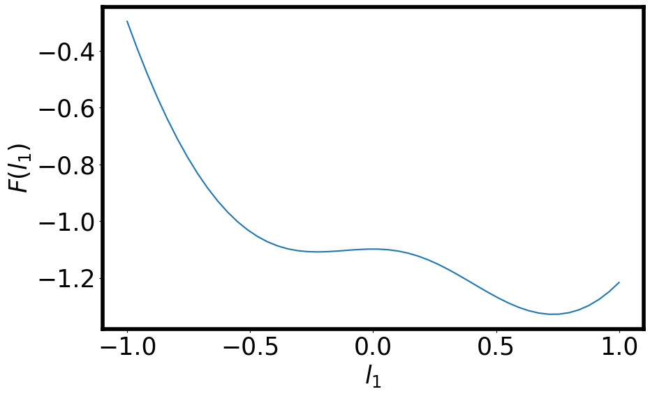
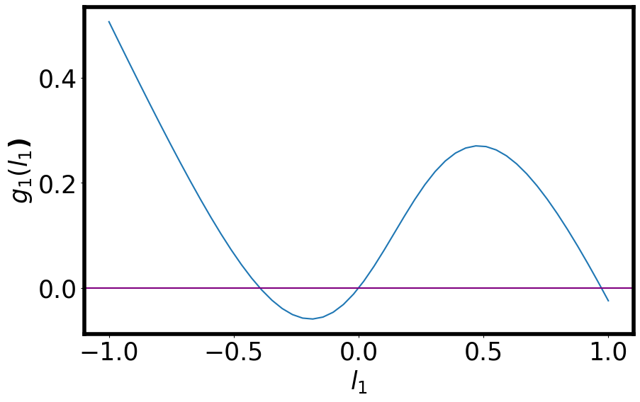
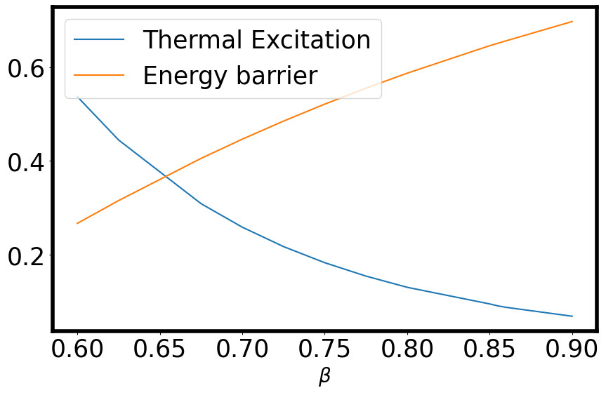
 a)                                                     b)                                                   c)                                               

Figure 4: 4 $F(l_{1},0)$ vs. $l_{1}$ 4 $g(l_{1})$ vs. $l_{1}$ with $\beta=0.82$ 4 Plot for finding $T_{SSB}$ for $q=3$ state clock model

For odd $q$, in the low-temperature regime (Fig. 3), we have one global minimum on the positive $l_{1}$-axis and one local maximum (between two consecutive global minima) on the negative $l_{1}$-axis. For illustration, we plot the low-temperature free energy as a function of $l_{1}$ keeping $l_{2}=0$ for the $q=3$ model (Fig. 4). In this plot, we see a global minimum and a local minimum, which is actually the local maximum while going from one to the next global minimum. We can calculate their positions along the $l_{1}$-axis by taking $\pdv{F(l_{1},0)}{l_{l}}=0$, where $F(l_{1},0)$ represents the free energy as function of $l_{1}$ keeping $l_{2}=0$.

For $q=3$, according to Eq. 11, the free energy function $F(l_{1},0)$ is

$$F(l_{1},0)=\frac{Jl^{2}_{1}r}{2}-\frac{\ln\sum_{i=1}^{3}e^{{\beta{Jr(l_{1}\cos{\frac{2\pi i}{q}})}}}}{\beta}.$$ (14)

Taking the partial derivative of $F(l_{1},0)$ w.r.t $l_{1}$, and equating it to zero, we get

$$l_{1}=\frac{\sum_{i=1}^{3}\cos{\frac{2\pi i}{3}}e^{\beta l_{1}Jr\cos{\frac{2\pi i}{3}}}}{\sum_{i=1}^{3}e^{\beta l_{1}Jr\cos{\frac{2\pi i}{3}}}}.$$ (15)

Considering $r=4$ and $J=1$, we obtain

$$l_{1}=\frac{e^{4\beta l_{1}}-e^{-2\beta l_{1}}}{e^{4\beta l_{1}}+2e^{-2\beta l_{1}}}.$$ (16)

This is a transcendental equation that can not be solved directly. We need to do some numerical calculations to solve this equation. Let

$$g(l_{1})=\frac{e^{4\beta l_{1}}-e^{-2\beta l_{1}}}{e^{4\beta l_{1}}+2e^{-2\beta l_{1}}}-l_{1}.$$ (17)

For a given $\beta$, the values of $l_{1}$ corresponding to the zeros of the function $g(l_{1})$ are the solutions of Eq. 16. These solutions can easily be found from the plot of $g(l_{1})$, as can be seen in Fig. 4. We clearly see that there are three solutions: one corresponds to the global minimum ($l_{1}>0$), the next one corresponds to the local maximum ($l_{1}=0$), and the last one corresponds to the local maximum between two consecutive minima ($l_{1}<0)$. Now, the energy barrier can be found by taking the difference between the global minimum and local maximum calculated from $F(l_{1},0)$ using appropriate $l_{1}$ values (solutions of Eq. 16). The energy barrier as a function of $\beta$ can be found in Fig. 4.

Now, for the calculation of thermal energy, we first calculate the internal energy of the spin by using the relation

$$U=\frac{\sum_{k=1}^{3}\epsilon(k)e^{-\beta\epsilon(k)}}{\sum_{k=1}^{3}e^{-\beta\epsilon(k)}},$$

where the expression of energy $\epsilon(k)$ can be found in Eq. 8 with $q=3$. Written explicitly, we have

$$U=\frac{2(2l^{2}_{1}+2l_{1})e^{-2l_{1}\beta}+(2l^{2}_{1}-4l_{1})e^{4\beta l_{1}}}{2e^{-2\beta l_{1}}+e^{4\beta l_{1}}}.$$ (18)

The order of thermal energy ($U-F$) at a global minimum is calculated using Eqs. 14 and 18 with the appropriate $l_{1}$ value coming from solving Eq. 16. The thermal energy as a function of $\beta$ can be found in Fig. 4. From this plot, we can easily check the temperature at which the thermal energy and the energy barrier match. We find that around $\beta=0.65$, they are equal; thus, for $q=3$, the symmetry-breaking phase transition temperature is $T_{SSB}=\frac{1}{0.65k_{B}}=\frac{1.538}{k_{B}}$. In the same way, we can calculate symmetry-breaking phase transition temperature for other odd $q-$state clock models. For $q=5$ and $7$, calculated $T_{SSB}$ values can be found in Table 1.

II.3.2 Calculation of $T_{SSB}$ when $q$ is even

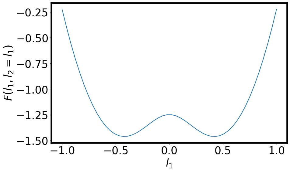
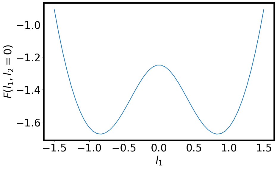
 a)                                                        b)                                                     

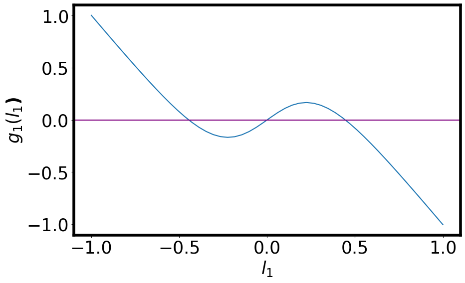
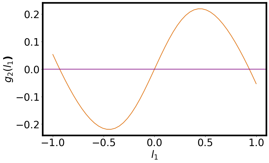
 c)                                                       d)                                                     

Figure 5: 5 $F(l_{1},l_{2}=l_{1})$ vs. $l_{1}$ 5 $F(l_{1},0)$ vs. $l_{1}$ 5 $g_{1}(l_{1})$ vs. $l_{1}$ 5 $g_{2}(l_{1})$ vs. $l_{1}$ with $\beta=0.82$

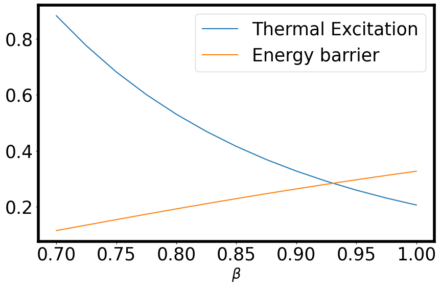
Figure 6: Plot for finding $T_{SSB}$ for $q=4$ state clock model

While calculating $T_{SSB}$ for the $q-$state clock model with even $q$, the trick used for odd $q$ will not work. If we plot the function $F(l_{1},0)$ with $l_{1}$ or plot $F(0,l_{2})$ with $l_{2}$, we will get two global minima (Fig. 5). However, we need the global minimum and the local maximum (between two successive global minima) to calculate the energy barrier between two successive global minima. To get the local maximum, we need to analyze the free energy along the line joining the origin and the midpoint between two consecutive global minima. For convenience, we can take the line joining the origin and the midpoint between the first two global minima (the first one being on the positive $l_{1}$-axis). The equation for this line is $l_{2}=l_{1}\tan{\frac{\pi}{q}}$. Along this line, the $F(l_{1},l_{2})$ plot can be seen in Fig. 5. Along this line, we can get the local maximum by solving the equation $\pdv{F}{l_{1}}=0$. Replacing $l_{2}$ by $l_{1}\tan{\frac{\pi}{q}}$ in the expression of $F(l_{1},l_{2})$, then following the procedure described for odd $q$, we get the following transcendental equation for $l_{1}$ (taking $q=4$ and $J=1$):

$$l_{1}=\frac{e^{4\beta l_{1}}-e^{-4\beta l_{1}}}{2(e^{4\beta l_{1}}+e^{-4\beta l_{1}})}.$$ (19)

To solve this equation for $l_{1}$, we define the following function,

$$g_{1}(l_{1})=\frac{e^{4\beta l_{1}}-e^{-4\beta l_{1}}}{2(e^{4\beta l_{1}}+e^{-4\beta l_{1}})}-l_{1}.$$ (20)

The roots of the equation $g_{1}(l_{1})=0$ are the solutions of Eq. 19. As can be seen from Fig. 5, there are three solutions. Two solutions for which $l_{1}\neq 0$ correspond to the local maxima (between global minima).

There are two global minima on the $l_{1}$-axis, as can be seen in Fig. 5; we can get them by solving $\pdv{F(l_{1},0)}{l_{1}}=0$. This leads to the following transcendental equation for $l_{1}$ (again taking $q=4$ and $J=1$):

$$l_{1}=\frac{e^{4\beta l_{1}}-e^{-4\beta l_{1}}}{2+(e^{4\beta l_{1}}+e^{-4\beta l_{1}})}$$ (21)

We now define the following function $g_{2}(l_{1})$ to find the solutions of the above equation,

$$g_{2}(l_{1})=l_{1}-\frac{e^{4\beta l_{1}}-e^{-4\beta l_{1}}}{2+(e^{4\beta l_{1}}+e^{-4\beta l_{1}})}.$$ (22)

We see from Fig. 5 that there are three solutions, two of them for which $l_{1}\neq 0$ corresponds to the global minima. The energy barrier can be found by taking the difference between the global minimum and local maximum of the free energy as calculated above. The energy barrier as a function of $\beta$ can be seen in Fig. 6.

Next, to estimate the thermal energy ($U-F$) at the global minimum, we need to calculate the internal energy $U$. The expression of $U$, in this case, is given by

$$U=\frac{4l^{2}_{1}+(2l^{2}_{1}+4l_{1})e^{-4\beta l_{1}}+(2l^{2}_{1}-4l_{1})e^{4\beta l_{1}}}{2+e^{-4\beta l_{1}}+e^{4\beta l_{1}}},$$ (23)

where $l_{1}$ corresponds to a global minimum. The details of how the internal energy is calculated are already discussed for the case of odd $q$. The thermal energy at a global minimum as a function of $\beta$ can be found in Fig. 6. From this figure, we can easily check at which temperature the thermal energy matches with the energy barrier; we see that, for $q=4$, two quantities match near $\beta=0.93$. We, therefore, estimate that $T_{SSB}=1.075/k_{B}$. We also calculated $T_{SSB}$ for $q=6$, which can be found in Table 1.

From this Table 1, we can see that the spontaneous symmetry-breaking phase transition temperature ($T_{SSB}$) decreases with an increase in $q$; this is also evident in Fig. 7. Although these results help us understand how $T_{SSB}$ changes with $q$, they do not reveal the exact functional dependence of the transition temperature on $q$. For a better understanding of the functional dependence, in the following, we use our mean-field theory to analytically estimate the value of $T_{SSB}$ in the large-$q$ limit.

$q$-value	$T_{SSB}$
3	$1.538/k_{B}$
4	$1.075/k_{B}$
5	$0.7692/k_{B}$
6	$0.556/k_{B}$
7	$0.4225/k_{B}$

Table 1: Numerically calculated $T_{SSB}$ values for different $q$ values

Figure 7: Plot for $T_{SSB}$ vs. $q$

II.4 Analytical calculation of $T_{SSB}$ in the large-$q$ limit

In this part, we first calculate the energy barrier, and then we calculate the thermal energy to estimate $T_{SSB}$ in the large-$q$ limit.

II.4.1 Calculation of energy barrier

For the large-$q$ limit, we can convert the summation appearing in the free energy expression, as seen in Eq.11, into an integration. Consequently, we have the following expression of the free energy,

$$F=\frac{J(l^{2}_{1}+l^{2}_{2})r}{2}-\frac{1}{\beta}\ln\int_{1}^{q}e^{{\beta{Jr(l_{1}\cos{\frac{2\pi j}{q}}+l_{2}\sin{\frac{2\pi j}{q}})}}}dj.$$ (24)

However, performing this integration is not straightforward. To go further, we represent the integrand function with a judiciously chosen simpler function. For even $q$, we first convert the integration limits to a more symmetric ones; accordingly,

$$F=\frac{J(l^{2}_{1}+l^{2}_{2})r}{2}-\frac{1}{\beta}\ln\int_{-\frac{q}{2}+1}^{\frac{q}{2}}e^{{\beta{Jr(l_{1}\cos{\frac{2\pi j}{q}}+l_{2}\sin{\frac{2\pi j}{q}})}}}dj.$$ (25)

If we are interested in calculating the global minima on the $l_{1}$-axis, we have to deal with the integrand function $e^{\beta{Jrl_{1}\cos{\frac{2\pi j}{q}}}}$. While replacing this function with a simpler function, we choose a function so that the extrema points of the original and the new function match. We note that the original function has a maximum at $j=0$ and the function effectively vanishes when $j>\frac{q}{4}$ or $j<-\frac{q}{4}$, since $\cos{\frac{2\pi j}{q}}$ picks up a negative sign in the ranges. With these properties in mind, we now replace this integrand function with the following approximate function:

$$e^{{\beta{Jrl_{1}\cos{\frac{2\pi j}{q}}}}}\to(1-cj^{2})e^{\beta{Jrl_{1}}}.$$

The value of $c$ is determined by the fact that the original function effectively vanishes at $j=\pm\frac{q}{4}$. This gives us $c=(\frac{4}{q})^{2}$. It may be mentioned here that the original and the approximate functions have the same maximum, and they effectively vanish at the same points. It is also worth commenting that the integration over the new approximate function should be performed only from $-\frac{q}{4}$ to $\frac{q}{4}$. With this judiciously chosen approximate function, it is now easy to estimate the value of the integral:

$${\int_{-\frac{q}{2}+1}^{\frac{q}{2}}e^{{\beta{Jr(l_{1}\cos{\frac{2\pi j}{q}})}}}dj}\to{\int_{-\frac{q}{4}}^{\frac{q}{4}}(1-{(\frac{4}{q})}^{2}j^{2})e^{\beta{Jrl_{1}}}dj}$$

$$=\frac{q}{3}e^{Jr\beta l_{1}}.$$

Using this result, the expression for the free energy $F$ along the $l_{1}$-axis can be written as,

$$F=\frac{Jl^{2}_{1}r}{2}-Jrl_{1}-\frac{\ln(\frac{q}{3})}{\beta}.$$ (26)

Now the global minimum can be found from $\pdv{F}{l_{1}}=0$. This gives us $l_{1}=1$ at the global minimum. So, the free energy at the global minimum is,

$$F_{G}=-\frac{Jr}{2}-\frac{1}{\beta}\ln(\frac{q}{3}).$$ (27)

For the calculation of the energy barrier, we next calculate the local maximum (between consecutive global minima). We note that if we connect by straight lines all the global minima to the origin ($l_{1}$=0, $l_{2}$=0), the angle between consecutive lines would be $\frac{2\pi}{q}$. Let us consider that the coordinate of the local maximum, between the first two global minima, is ($l_{1}$, $l_{2}$) and the coordinate of the global minimum, which is on the $l_{1}$-axis, is given by $(l,0)$. Some trigonometric considerations show that $l_{1}=l\cos^{2}{\frac{\pi}{q}}$ and $l_{2}=l\cos{\frac{\pi}{q}}\sin{\frac{\pi}{q}}$. Then, the expression for free energy, as seen in Eq. 25, at the local maximum will take the following form:

$$F=\frac{Jrl^{2}\cos^{2}{\frac{\pi}{q}}}{2}-\frac{1}{\beta}\ln\int_{-\frac{q}{2}+1}^{\frac{q}{2}}e^{{\beta{Jrl\cos{\frac{\pi}{q}}\cos{\frac{(2\pi j-\pi)}{q}}}}}dj.$$ (28)

Once again, we will replace the integrand function with a simpler function with the same extreme points. We note that the function $e^{\beta{Jrl\cos{\frac{\pi}{q}}\cos{\frac{(2\pi j-\pi)}{q}}}}$ vanishes when $j<\frac{-q}{4}+\frac{1}{2}$ or $j>\frac{q}{4}+\frac{1}{2}$, and has a maximum at $j=\frac{1}{2}$. But $j$ is always an integer, so we have to consider the nearest integer of $\frac{1}{2}$, which are 0 and 1 while approximating the function; accordingly, the new function will be defined in two regions: one is $(\frac{-q}{4}+\frac{1}{2})$ to 0, and the other one is from 1 to $(\frac{q}{4}+\frac{1}{2})$.

In the first interval, i.e. from $(\frac{-q}{4}+\frac{1}{2})$ to 0, we can approximate the function as $(1-cj^{2})e^{(Jr\beta l\cos^{2}{\frac{\pi}{q}})}$. Both the original function and this approximate function have the same maximum at $j=0$. The constant $c$ can be determined from the fact that the approximate function should vanish at $j=\frac{-q}{4}+\frac{1}{2}$. From this condition we get $c=(\frac{4}{q-2})^{2}$.

Similarly, for the second interval from j=1 to j=$(\frac{q}{4}+\frac{1}{2})$, we approximate the function as $(1-b(j-1)^{2})e^{(Jr\beta l\cos^{2}{\frac{\pi}{q}})}$ with $b=(\frac{4}{q-2})^{2}$. Thus, we get the following:

$$\int_{-\frac{q}{2}+1}^{\frac{q}{2}}e^{\beta{Jrl\cos{\frac{\pi}{q}}\cos{\frac{(2\pi j-\pi)}{q}}}}dj\to\int_{\frac{-q}{4}+\frac{1}{2}}^{0}(1-cj^{2})e^{(Jr\beta l\cos^{2}{\frac{\pi}{q}})}dj+\int_{1}^{\frac{q}{4}+\frac{1}{2}}(1-b(j-1)^{2})e^{(Jr\beta l\cos^{2}{\frac{\pi}{q}})}dj.$$ (29)

After performing the integration, we get the following:

$$\int_{-\frac{q}{2}+1}^{\frac{q}{2}}e^{\beta{Jrl\cos{\frac{\pi}{q}}\cos{\frac{(2\pi j-\pi)}{q}}}}dj\to\frac{q-2}{3}e^{(Jr\beta l\cos^{2}{\frac{\pi}{q}})}.$$ (30)

Thus, from Eq. 28, we get the following expression for the free energy at the local maximum,

$$F_{L}=\frac{Jrl^{2}\cos^{2}{\frac{\pi}{q}}}{2}-\frac{\ln{(\frac{q-2}{3}e^{(Jr\beta l\cos^{2}{\frac{\pi}{q}})})}}{\beta},$$ (31)

with $l=1$, as obtained earlier. Taking $\cos^{2}{\frac{\pi}{q}}\approx 1-\frac{\pi^{2}}{q^{2}}$ for large $q$, we get

$$F_{L}=-\frac{1}{2}Jr(1-\frac{\pi^{2}}{q^{2}})-\frac{1}{\beta}\ln{(\frac{q-2}{3})}.$$ (32)

From Eqs. 27 and 32, we now get an estimate for the energy barrier:

$$F_{L}-F_{G}=\frac{Jr\pi^{2}}{2q^{2}}-\frac{\ln{\frac{q-2}{3}}}{\beta}+\frac{\ln{\frac{q}{3}}}{\beta}.$$ (33)

II.4.2 Calculation of thermal energy

To calculate the thermal energy ($U-F$) at a global minimum, we use the following thermodynamic relation to first calculate the internal energy at the global minimum ($U_{G}$):

$$U_{G}=-T^{2}\frac{\partial}{\partial T}(\frac{F_{G}}{T}),$$ (34)

where $F_{G}$ is given by Eq. 27. A simple calculation shows that

$$U_{G}=-\frac{Jr}{2}.$$ (35)

Hence, the thermal energy at the global minimum is

$$U_{G}-F_{G}=\frac{1}{\beta}\ln(\frac{q}{3}).$$ (36)

II.4.3 Estimation of $T_{SSB}$

As discussed earlier, an estimation of the spontaneous symmetry-breaking transition temperature ($T_{SSB}$) can be found by equating the energy barrier between two consecutive global minima and the thermal energy at a global minimum. Accordingly, from Eqs. 33 and 36, we get

$$\frac{Jr\pi^{2}}{2q^{2}}-\frac{\ln{\frac{q-2}{3}}}{\beta}+\frac{\ln{\frac{q}{3}}}{\beta}=\frac{1}{\beta}\ln(\frac{q}{3}).$$

Solution of this equation gives (after replacing $\beta$ by $\frac{1}{k_{B}T_{SSB}}$),

$$T_{SSB}=\frac{Jr\pi^{2}}{2k_{B}q^{2}\ln\frac{q-2}{3}}.$$ (37)

For large-$q$, $q^{2}$ dominates over $\ln{\frac{q-2}{3}}$, so we see that $T_{SSB}$ decreases as $q^{-2}$, as expected earlier for large-$q$.

The zero-th-order mean-field theory that we discussed provides many insights into the $q$-state clock model. However, this theory does not allow us to estimate the important quantities like spin-spin correlation. To calculate this quantity, we now develop a higher-order mean-field theory where two neighboring spins with exact interaction are targeted. This higher-order theory also helps us improve some of the results we already obtained using the zero-th-order theory.

III Higher-order mean-field theory

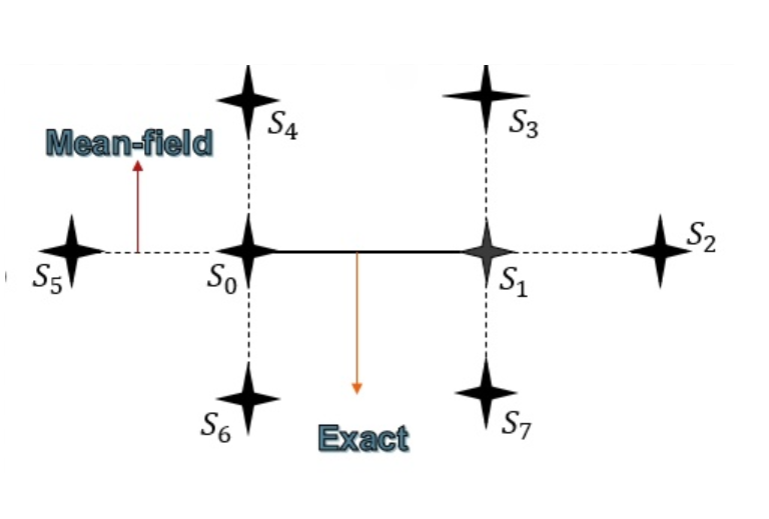
Figure 8: First order mean-field configuration

Let us consider a two-dimensional square lattice and focus on the two spins ($S_{0}$ and $S_{1}$) that interact exactly. These two spins are in the mean field created by their neighboring spins ($S_{2},S_{3},S_{4},S_{5},S_{6},S_{7}$), as shown in Fig. 8. The Hamiltonian for the system of two spins can be written as:

$$\begin{split}h_{01}=&-JRe(S_{0}S^{*}_{1}\\ &+\frac{1}{2}(S_{5}S^{*}_{0}+S_{1}S^{*}_{2}+S_{6}S^{*}_{0}+S_{0}S^{*}_{4}+S_{7}S^{*}_{1}+S_{1}S^{*}_{3})).\end{split}$$ (38)

The factor 1/2 is to avoid double counting the interactions between the targeted spins and their neighbors. If there are $N$ number of spins, then there are $\frac{N}{2}$ such spin pairs. We recall here that the complex spin variable ($S_{k}$) associated with the $k$-th spin is by definition: $S_{k}=e^{i\theta_{k}}$, where $\theta_{k}=2\pi j_{k}/q$. The variable $j_{k}$ takes any integer value from 1 to $q$. To develop the mean-field theory, we now replace a spin variable with a complex mean-field parameter ($l$) and a small fluctuation or deviation term: $S_{k}=l+\delta S_{k}$. We take a translationally invariant system for which the mean-field parameter $l$ is the same for all the spins. Using the parameter $l$, any interaction term can be approximated as: $S_{i}S_{j}^{*}\approx-|l|^{2}+l^{*}S_{i}+lS_{j}^{*}$. With the help of this expression, we get the following mean-field version of Hamiltonian in Eq. 38,

$$\begin{split}h_{MF}=&-JRe(S_{0}S_{1}^{*}\\ &-\frac{3}{2}|l|^{2}+\frac{3}{2}l^{*}S_{0}+\frac{1}{2}\sum_{j\in N_{0}}lS_{j}^{*}\\ &-\frac{3}{2}|l|^{2}+\frac{3}{2}l^{*}S_{1}+\frac{1}{2}\sum_{k\in N_{1}}lS_{k}^{*}).\end{split}$$ (39)

Here, $N_{0}$ denotes the set of nearest neighbors of the 0-th spin except the 1st spin. Similarly, $N_{1}$ is the set of nearest neighbors of the 1st spin except the 0-th spin. It may be mentioned here that since we are interested in the real part of an interaction term, terms like $l^{*}S_{0}$ and $lS_{0}^{*}$ can be taken to be equivalent and can be written interchangeably. From Eq. 39, if we now write the mean-field Hamiltonian for the whole two-dimensional system, we will have exact interaction terms like $S_{0}S_{1}^{*}$ corresponding to each target spin pair and the terms like $l^{*}S_{0}$ appearing 3 times in the Hamiltonian. Therefore, the total mean-field Hamiltonian of the system can be written as the sum of $N/2$ mean-field pair Hamiltonians; this mean-field pair Hamiltonian corresponding to $i-j$ pair (nearest neighbors) is given by,

$$h_{ij}=-JRe(S_{i}S_{j}^{*}-3|l|^{2}+3l^{*}S_{i}+3lS_{j}^{*}).$$ (40)

Now we recall that $S_{k}=\cos{\theta_{k}}+i\sin{\theta_{k}}$, where $\theta_{k}=2\pi j_{k}/q$ with $j_{k}$ taking values from 1 to $q$. If we write $l=l_{1}+il_{2}$, we get from Eq. 40:

$$\begin{split}h_{ij}=&-J\cos{(\theta_{i}-\theta_{j})}+3J(l_{1}^{2}+l_{2}^{2})\\ &-3Jl_{1}(\cos{\theta_{i}}+\cos{\theta_{j}})-3Jl_{2}(\sin{\theta_{i}}+\sin{\theta_{j}}).\end{split}$$ (41)

The possible energy values of the spin pair can be obtained from Eq. 41 by taking different possible values of $\theta_{i}$ and $\theta_{j}$. We can now calculate the partition function of the system as $Z=Z_{ij}^{\frac{N}{2}}$, where $Z_{ij}$ is the partition function corresponding to the pair $i-j$ and is given by,

$$Z_{ij}=\sum_{\theta_{i},\theta_{j}}e^{-\beta h_{ij}}.$$ (42)

Here, the sum is over possible values of $\theta_{i}$ and $\theta_{j}$. The free energy corresponding to a spin pair is given by,

$$F=-\frac{1}{\beta}\ln Z_{ij}.$$ (43)

Written explicitly, we get the following expression for the free energy,

$$F=3J(l_{1}^{2}+l_{2}^{2})-\frac{1}{\beta}\ln\sum_{i=1}^{q}\sum_{j=1}^{q}e^{J\beta(\cos{\frac{2\pi(i-j)}{q}}+3l_{1}(\cos{\frac{2\pi i}{q}+\cos{\frac{2\pi j}{q}})+3l_{2}(\sin{\frac{2\pi i}{q}}+\sin{\frac{2\pi j}{q}})})}.$$ (44)

III.1 Free energy plots at different temperatures

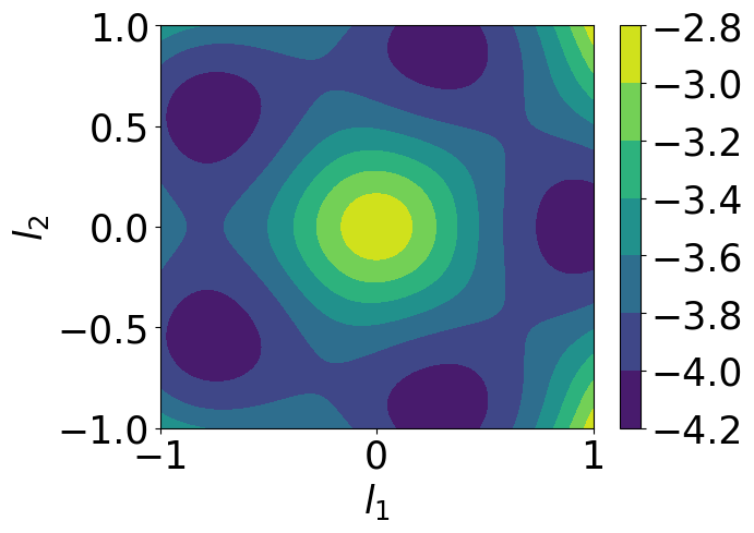
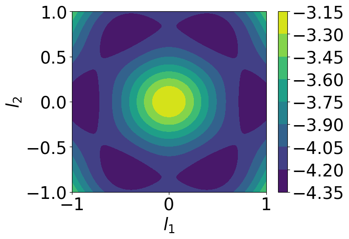
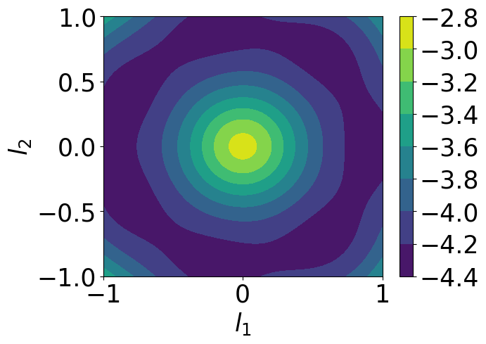
 a)                                                b)                                                 c)                                              

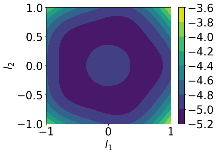
Figure 9: Free energy at low-temperature: 11 $q=5$, 11 $q=6$, 11 $q=7$.

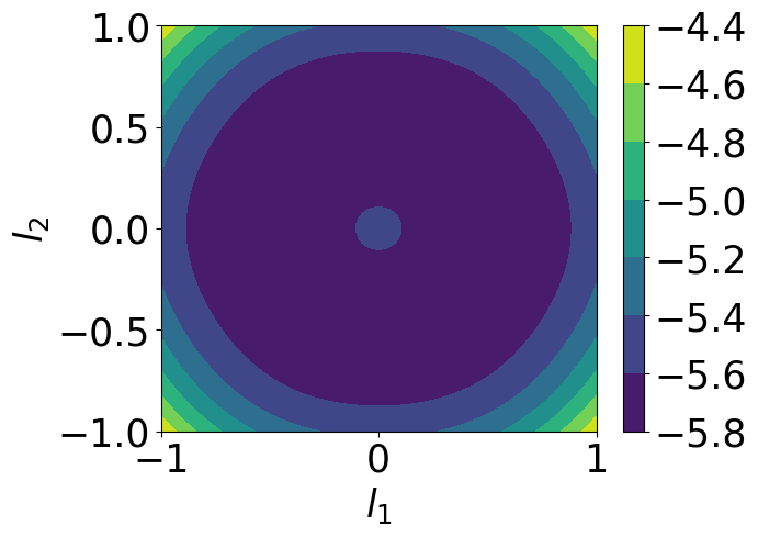
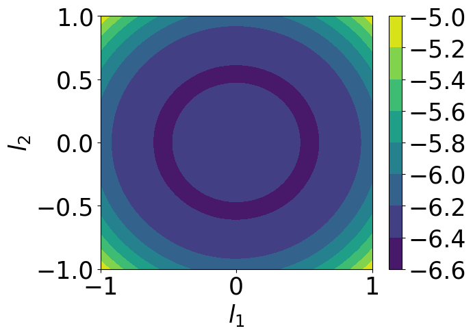
 a)                                              b)                                              c)                                            

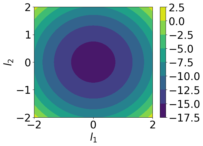
Figure 10: Free energy at intermediate-temperature: 11 $q=5$, 11 $q=6$, 11 $q=7$.

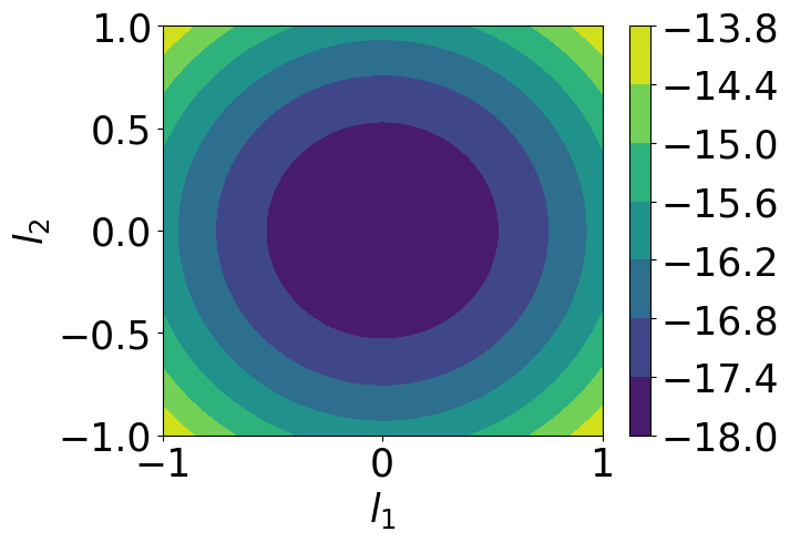
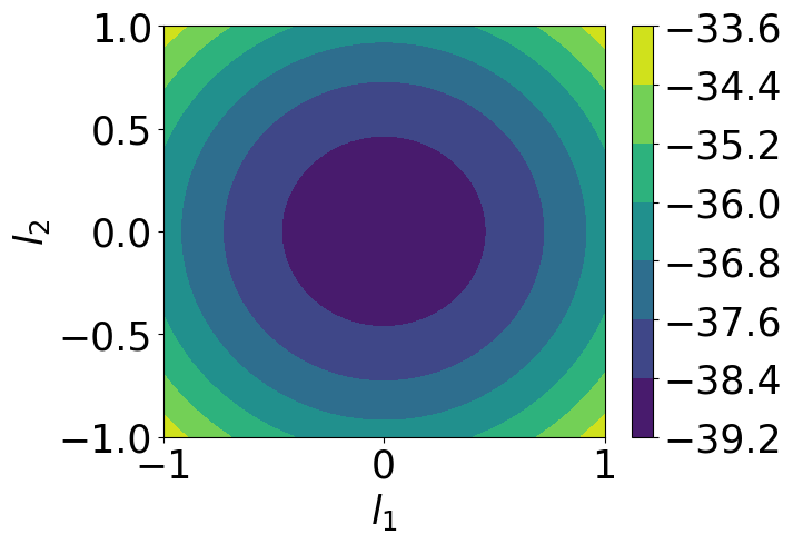
 a)                                            b)                                              c)                                            

Figure 11: Free energy at high-temperature: 12 $q=5$, 12 $q=6$, 11 $q=7$.

Using this new approximation, the behavior of free energy can be analyzed at a high temperature, intermediate temperature, and low temperature in a similar way as we have done previously (zeroth order mean-field approach). The free energy plots in three different temperature ranges for $q=$ 5, 6, and 7 can be found in Figs. 11], 11 and 11. These new results are qualitatively the same as obtained using the zeroth order theory. There are some quantitative differences, which can be appreciated from the updated value of $T_{BKT}$, which we again calculate in the following using the new mean-field approach.

III.2 Calculation of $T_{BKT}$ using new mean-field approximation

We can use the same scheme to calculate the BKT transition temperature as in the first part. We will find at which temperature the free energy function has an inflection point at (0,0). From Eq. 44, we have the free energy as function of $l_{1}$ ($l_{2}$=0) as follows:

$$\begin{split}F(l_{1},0)=&~{}3J|l_{1}|^{2}\\ &-\frac{1}{\beta}\ln\sum_{i=1}^{q}\sum_{j=1}^{q}e^{J\beta(\cos{\frac{2\pi(i-j)}{q}}+3l_{1}(\cos{\frac{2\pi i}{q}+\cos{\frac{2\pi j}{q}}))}}.\end{split}$$ (45)

Now taking the second order partial derivative of $F(l_{1},0)$ at $l_{1}=0$ and equating it to 0, we obtain:

$$\begin{split}\pdv[order={2}]{F}{l_{1}}_{l_{1}=0}&=6J+9\beta J^{2}\frac{\left(\sum_{i=1}^{q}\sum_{j=1}^{q}(\cos{\frac{2\pi i}{q}}+\cos{\frac{2\pi j}{q}})e^{\beta J\cos{\frac{2\pi(i-j)}{q}}}\right)^{2}}{\left(\sum_{i=1}^{q}\sum_{j=1}^{q}e^{\beta J\cos{\frac{2\pi(i-j)}{q}}}\right)^{2}}\\ &-9\beta J^{2}\frac{\sum_{i=1}^{q}\sum_{j=1}^{q}(\cos{\frac{2\pi i}{q}}+\cos{\frac{2\pi j}{q}})^{2}e^{\beta J\cos{\frac{2\pi(i-j)}{q}}}}{\sum_{i=1}^{q}\sum_{j=1}^{q}e^{\beta J\cos{\frac{2\pi(i-j)}{q}}}}=0.\end{split}$$ (46)

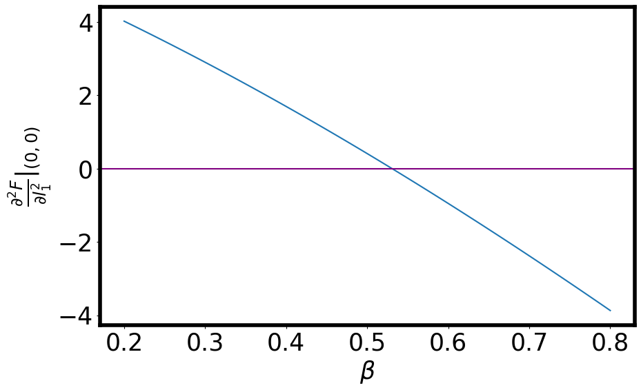
 a)                                                     b)                                                   

Figure 12: Plots of $\pdv[order={2}]{F}{l_{1}}_{l_{1}=0}$ vs. $\beta$ 12 for $q=6$ and 12 for $q=7$.

It is a nontrivial task to find $\beta$ for which the above equation (Eq. 46) is satisfied. To go further, we perform the following approximation. As seen in the first part, $\beta J\sim\frac{1}{2}$ near the BKT transition temperature. Therefore, near the transition temperature, $|\beta J\cos{\frac{2\pi(i-j)}{q}}|\lesssim\frac{1}{2}$. Accordingly, we take the following first order approximation: $e^{\beta J\cos{\frac{2\pi(i-j)}{q}}}\approx 1+\beta J\cos{\frac{2\pi(i-j)}{q}}$. Noting that $\sum_{i=1}^{q}\cos{\frac{2\pi i}{q}}=0$ and $\sum_{i=1}^{q}\cos^{2}{\frac{2\pi i}{q}}=\frac{q}{2}$, we get the following:

$$\begin{split}&\frac{\sum_{i=1}^{q}\sum_{j=1}^{q}(\cos{\frac{2\pi i}{q}}+\cos{\frac{2\pi j}{q}})^{2}e^{\beta J\cos{\frac{2\pi(i-j)}{q}}}}{\sum_{i=1}^{q}\sum_{j=1}^{q}e^{\beta J\cos{\frac{2\pi(i-j)}{q}}}}\\ &=\frac{\sum_{i=1}^{q}\sum_{j=1}^{q}(\cos{\frac{2\pi i}{q}}+\cos{\frac{2\pi j}{q}})^{2}(1+\beta J\cos{\frac{2\pi(i-j)}{q}})}{\sum_{i=1}^{q}\sum_{j=1}^{q}(1+\beta J\cos{\frac{2\pi(i-j)}{q}})}\\ &=\frac{q.\frac{q}{2}+q.\frac{q}{2}+2\beta J.\frac{q}{2}.\frac{q}{2}}{q.q}\\ &=1+\frac{\beta J}{2}.\end{split}$$ (47)

Using this result, we get from Eq. 46,

$$\begin{split}&6J+9\beta J^{2}\times 0-9\beta J^{2}(1+\frac{\beta J}{2})=0,~{}\text{i.e.,}\\ &4-6\beta J-3(\beta J)^{2}=0.\end{split}$$ (48)

Taking only the positive root of Eq. 48, we get the following value for the transition temperature (after replacing $\beta$ by $\frac{1}{k_{B}T_{BKT}}$),

$$T_{BKT}=\frac{1.895J}{k_{B}}.$$ (49)

Instead of solving Eq. 46 analytically by taking some approximation, it is also possible to directly solve the equation numerically. For given $q$, we can numerically check at which $\beta$ the equation is satisfied. For $q=$ 6 and 7, plots of $\pdv[order={2}]{F}{l_{1}}_{l_{1}=0}$ vs. $\beta$ can be seen Fig. 12. Numerical value of $T_{BKT}$ calculated from such plots show that $T_{BKT}=\frac{1.895J}{k_{B}}$ for $q=7$ or more, and this value of the transition temperature does not change much with $q$.

We note that, compared to the zeroth order result, the current value of $T_{BKT}$ is slightly closer to the reported value of $0.893J/k_{B}$ as found using Monte Carlo calculations [16]. Thus, we see that the consideration of a single exact interaction in the higher-order mean-field theory improves the results quantitatively.

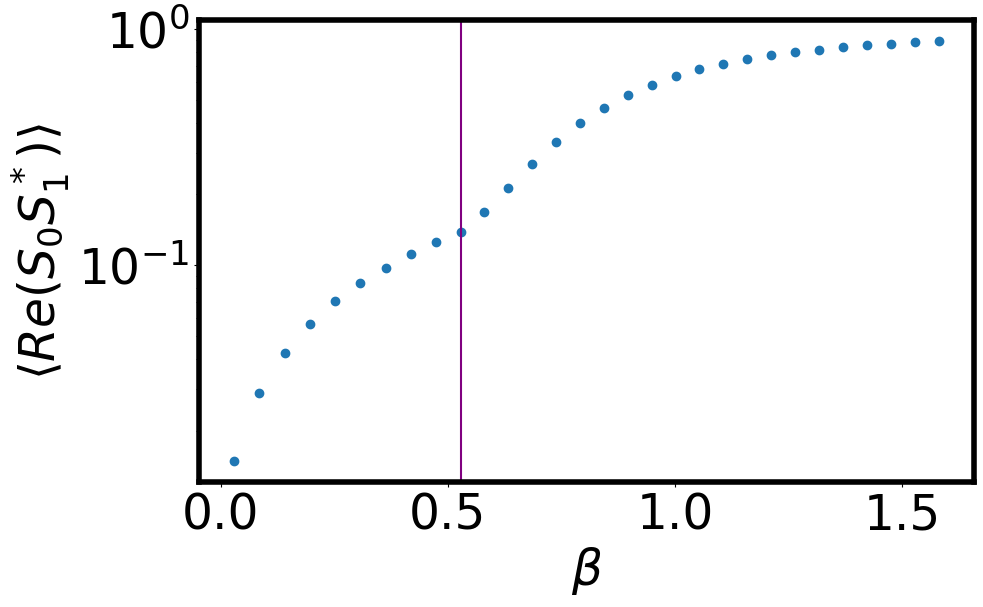
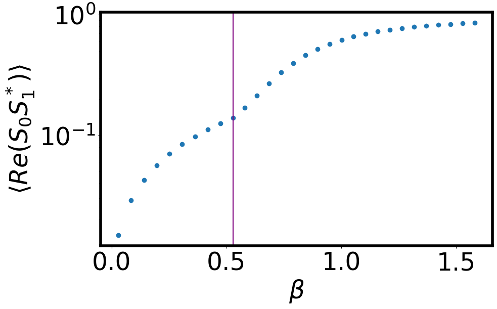
 a)                                                        b)                                                      

Figure 13: NN spin-spin correlation for 13 $q=6$, and 13 $q=7$.

III.3 Estimation of the spin-spin correlation

The spin-spin correlation is an important quantity in studying different phases of a system. The correlation shows different behaviors in different phases, and a change in its behavior normally indicates a phase transition. Mean-field theories, in general, do not predict exact correlation behavior. Our first-order mean-field theory considers one exact interaction between two neighboring spin pairs. As a result, it is possible to estimate the nearest-neighbor spin-spin correlation using this approach. Nearest-neighbor correlation can tell us whether the system is in an ordered or disordered phase at a given temperature. Using our first-order mean-field theory, we estimate the nearest-neighbor (NN) spin-spin correlation for the $q$-state clock model. We note that the NN spin-spin correlation is given by,

$$\langle Re(S_{0}S^{*}_{1})\rangle=\frac{\sum_{\theta_{0}}\sum_{\theta_{1}}Re(S_{0}S^{*}_{1})e^{-\beta h_{01}}}{\sum_{\theta_{0}}\sum_{\theta_{1}}e^{-\beta h_{01}}}.$$ (50)

Here $h_{01}$ is given by Eq. 41 with indices $i$ and $j$ taking values 0 and 1 respectively. In terms of variables $\theta_{0}$ and $\theta_{1}$, we also have $Re(S_{0}S^{*}_{1})=\cos{(\theta_{0}-\theta_{1})}$. Evaluating this correlation analytically is, in general, difficult. It is, though, possible to numerically evaluate the value of NN correlation at different values of $\beta$. Since the parameters $l_{1}$ and $l_{2}$ appear in $h_{01}$, to evaluate $\langle Re(S_{0}S^{*}_{1})\rangle$, we first need to find the numerical values of the parameters $l_{1}$ and $l_{2}$ at different $\beta$ values. We note from the free energy plots (Figs. 11, 11 and 11) that there is always a minimum on the $l_{1}$-axis. In the high-temperature limit, the minima are at the origin ($l_{1}=l_{2}=0$). There are $q$ minima around the origin in the low-temperature limit, but there is always one minimum on the positive $l_{1}$-axis. In the intermediate temperature, a ring of minima is around the origin. This allows us to take $l_{2}=0$ and an appropriate value of $l_{1}$ in $h_{01}$. To find this appropriate value of $l_{1}$ at a given $\beta$, we numerically find the free energy minimum on the $l_{1}$-axis from the equation $\pdv{F(l_{1},0)}{l_{1}}=0$, where $F(l_{1},0)$ is given by Eq. 45. For $q=6$ and 7, we calculate $l_{1}$ corresponding to the minimum on the $l_{1}$-axis for different $\beta$ values and then use that to calculate NN correlation at those $\beta$ values. Results can be seen in Fig. 13. We observe from the plots of NN correlation that there is a kink near $T_{BKT}=\frac{1.895J}{k_{B}}$. This result correctly predicts a change in phase at $T_{BKT}$. We, though, do not observe any noticeable change in correlation at $T_{SSB}$.

We now analytically calculate $\langle Re(S_{0}S^{*}_{1})\rangle$ in the high- and low-temperature limits.

III.3.1 NN correlation in high-temperature limit

We know from the free energy plots (Fiq. 11) that, in the high-temperature limit, there is only one minimum corresponding to $l_{1}=l_{2}=0$. Accordingly, we can evaluate Eq. 50 by taking $l_{1}=l_{2}=0$ in the Hamiltonian $h_{01}$ expression. Thus, in this temperature limit, $h_{01}=-J\cos{(\theta_{0}-\theta_{1})}$ and $e^{-\beta h_{01}}\approx 1+\beta J\cos{(\theta_{0}-\theta_{1})}$, since $\beta$ is small. Written explicitly, we get from Eq. 50,

$$\begin{split}\langle Re(S_{0}S^{*}_{1})\rangle=&\frac{\sum_{\theta_{0}}\sum_{\theta_{1}}\cos{(\theta_{0}-\theta_{1})}(1+\beta J\cos{(\theta_{0}-\theta_{1})})}{\sum_{\theta_{0}}\sum_{\theta_{1}}(1+\beta J\cos{(\theta_{0}-\theta_{1})})}\\ =&\frac{\sum_{i=1}^{q}\sum_{j=1}^{q}\cos{\frac{2\pi(i-j)}{q}}(1+\beta J\cos{\frac{2\pi(i-j)}{q}})}{\sum_{i=1}^{q}\sum_{j=1}^{q}(1+\beta J\cos{\frac{2\pi(i-j)}{q}})}.\end{split}$$ (51)

Noting the identities $\sum_{i=1}^{q}\cos{\frac{2\pi i}{q}}=0$ and $\sum_{i=1}^{q}\cos^{2}{\frac{2\pi i}{q}}=\frac{q}{2}$, we finally get

$$\langle Re(S_{0}S^{*}_{1})\rangle=\frac{\beta J}{2}.$$ (52)

We note here that, in the high-temperature limit, the NN spin-spin correlation decreases with increasing temperature. This is indeed what is expected in the disordered phase. In accordance with our analytical result, we also note from Fig. 13 that the NN correlation near the origin is linear with $\beta$.

III.3.2 NN correlation in low temperature limit

In the low-temperature limit, $\beta$ is large, and $l_{1}\to 1$ corresponds to the free energy minimum on the $l_{1}$ axis. In this limit, it is not possible to approximate $e^{-\beta h_{01}}$ by retaining a couple of terms from its (Taylor) series. To go further, for large q, we transform the summation to integration. With $l_{1}=1$ and $l_{2}=0$ in Eq. 41, we have

$$h_{01}=-J\cos{({\theta_{0}-\theta_{1}})}+3J-3J(\cos{\theta_{0}}+\cos{\theta_{1}}),$$ (53)

with the indices $i$ and $j$ taking their values 0 and 1, respectively. In the large $q$ limit and taking symmetric ranges for the integration variables $\theta_{0}$ and $\theta_{1}$, we get from Eq. 50,

$$\langle Re(S_{0}S^{*}_{1})\rangle=\frac{\int_{\theta_{0}=-\pi}^{\pi}\int_{\theta_{1}=-\pi}^{\pi}\cos{(\theta_{0}-\theta_{1})}e^{-\beta h_{01}}d\theta_{0}d\theta_{1}}{\int_{\theta_{0}=-\pi}^{\pi}\int_{\theta_{1}=-\pi}^{\pi}e^{-\beta h_{01}}d\theta_{0}d\theta_{1}},$$ (54)

where $h_{01}$ is given by Eq. 53. This can be further written as:

$$\langle Re(S_{0}S^{*}_{1})\rangle=\lim_{x\to 1}\frac{1}{\beta J}\pdv{}{x}\ln{\left(\int_{-\pi}^{\pi}\int_{-\pi}^{\pi}E(\theta_{0},\theta_{1};x)d\theta_{0}d\theta_{1}\right)},$$ (55)

where $E(\theta_{0},\theta_{1};x)=e^{J\beta(x\cos{(\theta_{0}-\theta_{1})}+3(\cos{\theta_{0}}+\cos{\theta_{1}}))}$. We now approximate the function $E(\theta_{0},\theta_{1};x)$ in a manner similar to how in the first part we approximated an exponential function by a second order polynomial. We note that function like $e^{t\cos{\theta}}$, with $t>0$, has a maximum $e^{t}$ at $\theta=0$. This exponential function effectively vanishes when $\theta\leq-\frac{\pi}{2}$ or $\theta\geq\frac{\pi}{2}$. For large $t$, this allows us to approximate the function as $e^{t\cos{\theta}}\approx e^{t(1-\theta^{2}/2)}\to e^{t}(1-tA\theta^{2})$. If $t$ is a given constant, $A$ is determined by the fact that at $\theta=\pm\frac{\pi}{2}$, the approximate function should vanish. If $t$ is a variable, then $A$ is determined by replacing $t$ by its limiting value and making sure that the approximate function vanishes at $\theta=\pm\frac{\pi}{2}$. It may be noted here that the original exponential function and the approximate polynomial function both have the same maximum at $\theta=0$.

Above discussion helps us to approximate $E(\theta_{0},\theta_{1};x)$ in the following way:

$$E(\theta_{0},\theta_{1};x)\to e^{\beta J(x+6)}(1-xA(\theta_{0}-\theta_{1})^{2})(1-B\theta_{0}^{2})(1-C\theta_{1}^{2}).$$ (56)

With this approximation, the integration ranges in Eq. 55 should be taken appropriately. First we now determine the values of the constants $A$, $B$ and $C$. The constants $B$ and $C$ are determined by making sure that the approximate function should vanish at $\theta_{0}=\pm\frac{\pi}{2}$ and $\theta_{1}=\pm\frac{\pi}{2}$. This gives us $B=C=(\frac{2}{\pi})^{2}$. While determining the constant $A$, we note that while $\theta_{0}=\theta_{1}$ corresponds to the maximum for both exponential and the approximate polynomial function, both functions should vanish when $|\theta_{0}-\theta_{1}|\geq\frac{\pi}{2}$. Since finally we are going to take the limit $x\to 1$, we determine that $A=(\frac{2}{\pi})^{2}$.

To find the appropriate ranges of integrations in Eq. 55 after replacing $E(\theta_{0},\theta_{1};x)$ by its approximation, we first note that the function $e^{3\beta J\cos{\theta_{0}}}$ or $e^{3\beta J\cos{\theta_{1}}}$ effectively vanishes when $|\theta_{0}|\geq\frac{\pi}{2}$ or $|\theta_{1}|\geq\frac{\pi}{2}$. On the other hand, the function $e^{x\beta J\cos{(\theta_{0}-\theta_{1})}}$ effectively vanishes when $|\theta_{0}-\theta_{1}|\geq\frac{\pi}{2}$. This tells us that, when $-\frac{\pi}{2}\leq\theta_{0}\leq 0$, the range of the other variable should be $-\frac{\pi}{2}\leq\theta_{1}\leq\frac{\pi}{2}+\theta_{0}$. Similarly, when $0\leq\theta_{0}\leq\frac{\pi}{2}$, the range of the other variable should be $-\frac{\pi}{2}+\theta_{0}\leq\theta_{1}\leq\frac{\pi}{2}$.

Let us denote the approximate function by $\tilde{E}(\theta_{0},\theta_{1};x)$, i.e.,

$$\tilde{E}(\theta_{0},\theta_{1};x)=e^{\beta J(x+6)}(1-\frac{4x}{\pi^{2}}(\theta_{0}-\theta_{1})^{2})(1-\frac{4\theta_{0}^{2}}{\pi^{2}})(1-\frac{4\theta_{1}^{2}}{\pi^{2}}).$$ (57)

Now to find the NN correlation using Eq. 55, we need to perform the following integration,

$$\begin{split}I(x)=\int_{\theta_{0}=-\frac{\pi}{2}}^{0}\int_{\theta_{1}=-\frac{\pi}{2}}^{\frac{\pi}{2}+\theta_{0}}\tilde{E}(\theta_{0},\theta_{1};x)d\theta_{0}d\theta_{1}\\ +\int_{\theta_{0}=0}^{\frac{\pi}{2}}\int_{\theta_{1}=-\frac{\pi}{2}+\theta_{0}}^{\frac{\pi}{2}}\tilde{E}(\theta_{0},\theta_{1};x)d\theta_{0}d\theta_{1}.\end{split}$$ (58)

We find that $I(x)=(3.863-0.9678x)e^{\beta J(x+6)}$. We now have,

$$\begin{split}\langle Re(S^{*}_{0}S_{1})\rangle&=\lim_{x\to 1}\frac{1}{\beta J}\frac{\partial\ln{I(x)}}{\partial x}\\ &=1-\frac{1}{3\beta J}.\end{split}$$ (59)

As expected in the low-temperature regime, the NN spin-spin correlation saturates to the value 1 as the temperature reduces (i.e., $\beta\to\infty$). This analytical result matches well with our numerical results shown in Fig. 13.

IV Conclusion

The $q$-state is equivalent to the Ising model when $q=2$ and is equivalent to the $XY$ model when $q\to\infty$. In these two limits the model, respectively, shows the second order and the Berezinskii-Kosterlitz-Thouless (BKT) type transitions. The $q$-state clock model garnered a lot of interest due to the fact that it shows two different types of phase transitions for finite $q$ in two-dimension (2D). Except for a few special values of $q$, the 2D model is not exactly solvable. Different numerical techniques are developed to gain insights into the properties of this model. To investigate some of the unanswered questions and to address some of the debates in this field, we develop a mean-field theory (both basic and higher order) to study the $q$-state clock model. To the best of our knowledge, this is the first systematic mean-field study of the model with finite $q$. In our mean-field approach, spins are converted to complex spin variables, and the mean-field parameter is the mean of such a complex spin variable. Effectively, our theory has one complex mean-field parameter or, equivalently, two real parameters.

With our mean-field approach, we find that the system with finite $q$ shows two phase transitions - one at higher temperature is of BKT type while the other one -there are varying opinions about its nature- is found here to be spontaneous symmetry-breaking (SSB) type. Our basic mean-field approach shows that the BKT transition temperature ($T_{BKT}$) is $q$-independent, and it is found to be $T_{BKT}=\frac{2J}{k_{B}}$. We also find that the transition at lower temperatures decreases with increasing $q$ and found out to be $T_{SSB}\propto\frac{1}{q^{2}}$, with a weak logarithmic correction. This result is consistent with the fact that the $q$-state clock model is equivalent to the $XY$ model in the $q\to\infty$ limit, where we see only the BKT type transition.

In the second part of the paper, we develop a higher-order mean-field theory where the interaction between two targeted nearest neighbor spins is treated exactly. This improves our results quantitatively. For example, we recalculated the BKT transition temperature, and it comes out to be $T_{BKT}=\frac{1.895J}{k_{B}}$. This value is slightly closer to the original reported value of $\frac{0.893J}{k_{B}}$. The main advantage of this higher-order theory is that one can now estimate the nearest neighbor (NN) spin-spin correlation. Our numerical results show a clear change in the NN correlation at $T_{BKT}$ temperature. Our analytical results for the NN correlation in the high- and low-temperature limits are in accordance with what is expected for disordered and ordered phases, respectively.

There is a critical value of $q$, below which the 2D clock model only shows second-order phase transition, and when $q$ is above or equal to this critical value, we see two phase transitions - a BKT type transition at higher temperature and a second order transition at lower temperature. This critical value is known to be 5 ($q_{c}=5$). Our mean-field theory could not determine any critical value of $q$. In general, as mentioned before, the mean-field theory works better for large values of $q$. In the future, it will also be interesting to see if this mean-field theory or any variant of this can be used to get any deeper insights into the phase that appears between two different types of transition.

Author contributions: RK and MG calculated the BKT transition temperature using the zeroth order mean-field theory, AG performed rest of the analytical and numerical calculations using the zeroth and higher order mean-field theories, SS proposed the project and closely supervised the calculations, AG and SS wrote the manuscript.

References

- Baxter [1973] R. J. Baxter, Potts model at the critical temperature, Journal of Physics C: Solid State Physics 6, L445 (1973).
- Wu [1982] F. Y. Wu, The potts model, Rev. Mod. Phys. 54, 235 (1982).
- Chen et al. [2017] J. Chen, H.-J. Liao, H.-D. Xie, X.-J. Han, R.-Z. Huang, S. Cheng, Z.-C. Wei, Z.-Y. Xie, and T. Xiang, Phase transition of the q-state clock model: Duality and tensor renormalization, Chinese Physics Letters 34, 050503 (2017).
- Negrete et al. [2021] O. A. Negrete, P. Vargas, P. F. J, G. Saravia, and E. E. Vogel, Short-range berezinskii-kosterlitz-thouless phase characterization for the q-state clock model, Entropy 23, 1019 (2021).
- Li et al. [2020] Z.-Q. Li, L.-P. Yang, Z. Y. Xie, H.-H. Tu, H.-J. Liao, and T. Xiang, Critical properties of the two-dimensional -state clock model, Phys. Rev. E 101, 060105 (2020).
- Beale and Pathria [2011] P. D. Beale and R. K. Pathria, Statistical Mechanics, 3rd ed. (Elsevier, 2011).
- Kosterlitz [2016] J. M. Kosterlitz, Kosterlitz–thouless physics: a review of key issues, Reports on Progress in Physics 79, 026001 (2016).
- Onsager [1944] L. Onsager, Crystal statistics. i. a two-dimensional model with an order-disorder transition, Phys. Rev. 65, 117 (1944).
- Mermin and Wagner [1966] N. D. Mermin and H. Wagner, Absence of ferromagnetism or antiferromagnetism in one- or two-dimensional isotropic heisenberg models, Phys. Rev. Lett. 17, 1133 (1966).
- Berezinskii [1971] Berezinskii, Destruction of long-range order in one-dimensional and two-dimensional systems having a continuous symmetry group i. classical systems, Sov. Phys. JETP 32, 493 (1971).
- Kosterlitz [1974] J. M. Kosterlitz, The critical properties of the two-dimensional xy model, J. Phys. C 7, 1046 (1974).
- Kosterlitz and Thouless [1973] J. M. Kosterlitz and D. J. Thouless, Ordering, metastability and phase transitions in two-dimensional systems, Journal of Physics C: Solid State Physics 6, 1181 (1973).
- Gupta et al. [1988] R. Gupta, J. DeLapp, G. G. Batrouni, G. C. Fox, C. F. Baillie, and J. Apostolakis, Phase transition in the 2 d xy model, Physical review letters 61, 1996 (1988).
- Chen et al. [2022] H. Chen, P. Hou, S. Fang, and Y. Deng, Monte carlo study of duality and the berezinskii-kosterlitz-thouless phase transitions of the two-dimensional -state clock model in flow representations, Phys. Rev. E 106, 024106 (2022).
- Ortiz et al. [2012] G. Ortiz, E. Cobanera, and Z. Z. Nussinov, Dualities and the phase diagram of the p-clock model, Nuclear Physics B 854, 780 (2012).
- Hsieh et al. [2013] Y.-D. Hsieh, Y.-J. Kao, and A. W. Sandvik, Finite-size scaling method for the berezinskii-kosterlitz-thouless transition, J. Stat. Mech.: Theory Exp. , P09001.
- Ashkin and Teller [1943] J. Ashkin and E. Teller, Statistics of two-dimensional lattices with four components, Phys. Rev. 64, 178 (1943).
- Kihara et al. [1954] T. Kihara, Y. Midzuno, and T. Shizume, Statistics of two-dimensional lattices with many components, Journal of the Physical Society of Japan 9, 681 (1954).
- Kim and Joseph [1974] D. Kim and R. Joseph, Exact transition temperature of the potts model with q states per site for the triangular and honeycomb lattices, Journal of Physics C: Solid State Physics 7, L167 (1974).
- van der Sijs [1993] A. J. van der Sijs, Heisenberg models and a particular isotropic model, Physical Review B 48, 7125 (1993).
- Suzuki and Kubo [1968] M. Suzuki and R. Kubo, Dynamics of the ising model near the critical point. i, Journal of the Physical Society of Japan 24, 51 (1968).
- Tobochnik [1982] J. Tobochnik, Properties of the q-state clock model for q= 4, 5, and 6, Physical Review B 26, 6201 (1982).
- Gross et al. [1985] D. J. Gross, I. Kanter, and H. Sompolinsky, Mean-field theory of the potts glass, Physical Review Letters 55, 304 (1985).
- Brush [1967] S. G. Brush, History of the lenz-ising model, Reviews of modern physics 39, 883 (1967).
- Wang and Xiang [1997] X. Wang and T. Xiang, Transfer-matrix density-matrix renormalization-group theory for thermodynamics of one-dimensional quantum systems, Physical Review B 56, 5061 (1997).
- Kitanine et al. [2002] N. Kitanine, J. Maillet, N. Slavnov, and V. Terras, Spin–spin correlation functions of the xxz-12 heisenberg chain in a magnetic field, Nuclear Physics B 641, 487 (2002).
- [27] S. Ahamed, S. Cooper, V. Pathak, and W. Reeves, The berezinskii-kosterlitz-thouless transition, Dept. of Physics Astronomy, University of British Columbia, Canada .
- Kawasaki [1966] K. Kawasaki, Diffusion constants near the critical point for time-dependent ising models. i, Physical Review 145, 224 (1966).
- Kramers and Wannier [1941] H. A. Kramers and G. H. Wannier, Statistics of the two-dimensional ferromagnet. part i, Physical Review 60, 252 (1941).
- Alcaraz and Koberle [1980] F. Alcaraz and R. Koberle, Duality and the phases of z (n) spin systems, Journal of Physics A: Mathematical and General 13, L153 (1980).