Gravitating Skyrmions with localized fermions

Abstract

We consider self-gravitating Skyrmions in the presence of Dirac fermions, that carry spin and isospin. By varying the gravitational and the Yukawa coupling constants, we investigate the spectral flow of the fermion eigenvalue associated with a zero mode in the absence of gravity. We demonstrate that the backreaction of the fermion can strongly influence the Skyrmion-fermion configurations. In particular, the energy conditions may be violated, and regular anti-gravitating asymptotically flat solutions with negative ADM mass may emerge.

I Introduction

For a long time now, much attention has been paid to soliton solutions of various classical field theories. These are regular localized field configurations with finite energy. Well known examples of such topological solitons in (3+1)-dimensions are monopoles in the Yang-Mills-Higgs model [1, 2], Skyrmions [3, 4] and Hopfions [5, 6] (for reviews, see, for example, Refs. [7, 8]). In particular, the groundbreaking work by Skyrme [3, 4] gave rise to an increasing interest in the study of various aspects of such solutions in a wide variety of physical systems, both in flat and curved spacetime.

Flat space topological solitons can be minimally coupled to gravity. The emerging systems of the Einstein-matter field equations may then support the existence of gravitating spatially localized globally regular solutions. Endowing these gravitating soliton solutions with an event horizon, the so-called hairy black holes arise, which possess nontrivial matter fields outside their event horizon, i.e., they carry hair (see, e.g., Refs. [9, 10]). Well known examples include black holes within monopoles [11, 12, 13] and Skyrmions [14, 15, 16, 17, 18, 19].

A notable feature of topological solitons is the remarkable relation between the topological charge of the configuration and the fermionic zero modes localized on the soliton, provided by the fundamental Atiyah-Patodi-Singer index theorem [20]. In particular, in the background of a soliton of topological degree one the fermion spectrum exhibits a spectral flow of the eigenvalues with a normalizable bound mode crossing zero.

Study of the localization of fermionic modes on solitons started with the pioneering work of fermion bound states on a vortex line [21], and was followed by the investigation of fermion bound states on kinks [22, 23, 24], sphalerons [23, 25, 26], monopoles [27], Skyrmions [28, 29, 30], and domain walls [31]. Highlights of those and related studies include the appearance of fractional fermion number of solitons [22, 32], monopole catalysis of proton decay [33, 34], or the emergence of superconducting cosmic strings [35].

The nature of the fermionic zero modes depend on the associated solitons. For instance, for monopoles one finds an exact zero mode localized on them, irrespective of the strength of the Yukawa coupling [22]. For Skyrmions, in contrast, one observes spectral flow of the eigenvalues [28, 29, 30]. The fermion eigenvalue then depends crucially on the value of the Yukawa coupling, emerging from the positive continuum at a critical value of the coupling strength, then crossing zero at some other particular value and finally approaching the negative continuum.

While it is natural to first explore the properties of fermions in the background of the solitons, a subsequent investigation of the backreaction of the fermions on the solitons is called for, in particular, when the fermion-soliton coupling is no longer weak. In such a case, the properties of the solitons may be significantly affected. Examples range from the distortion of domain walls [36], kinks [37, 38], Skyrmions [39], and $CP^{2}$ solitons [40], via the emergence of soliton bound states [41, 42], to the outcome of soliton collisions [43, 44, 45], where the inclusion of the Dirac sea may possibly mitigate the effects somewhat [46, 47].

When including gravity, one needs to take into account the fundamental quantum character of the fermions [48]. This is typically done by describing the Dirac field with normalized wave functions, and by imposing the Pauli principle via the appropriate particle numbers of the considered states. The basic approximation scheme employed in the literature then consists of (i) considering only single-particle fermion states, (ii) ignoring second quantization of the fields, (iii) treating gravity only classically.

Based on this approximation scheme, for instance, fermions were studied in the background of the Einstein-Yang-Mills sphaleron barrier and the level crossing phenomenon was observed [49], with a fermionic zero mode at the top of the barrier, very much in analogy with the electroweak case [50]. The dynamical evolution of the fermionic zero mode localized on the self-gravitating $SU(2)$ monopole was studied in Ref. [51]. Considering only the Einstein-Dirac equations, the existence of regular localized configurations was shown in Ref. [52]. In fact, such configurations, the so-called Dirac stars, share a number of properties with boson stars [53, 54, 55, 56]. Interestingly, self-gravitating fermions may affect the metric dramatically, leading to significant violations of the energy conditions and allowing for (traversable) wormholes [57, 58, 59, 60]. Violation of the energy conditions by spinor fields was also seen to give rise to notable effects in cosmology [61, 62].

Here we consider in detail the spectral flow of the gravitating Skyrmion-fermion system [63], where the spherically symmetric fermionic mode is occupied by a single fermion, that backreacts on the gravitating Skyrmion. Without the fermion, the gravitating Skyrmion exhibits two branches of solutions. The lower mass Skyrmion branch starts from the flat space soliton, and merges with the higher mass Bartnik-McKinnon (BM) branch at a maximal value of the gravitational coupling constant [15, 18, 17, 19, 64]). Since in flat space the Skyrmion-fermion system exhibits spectral flow, when the Yukawa coupling is varied, it is interesting to investigate the effect of gravity on the spectral flow of the backreacting Skyrmion-fermion system.

The paper is organized as follows: We start with a brief description of the theoretical setting in section 2, where we present the action, the Ansatz for the fields, the resulting set of coupled equations, and the boundary conditions. In section 3 we discuss the numerical approach. Subsequently we give a detailed discussion of the numerical results. We end with our conclusions in section 4.

II Theoretical Setting

II.1 Einstein-Skyrme-Dirac Action

We consider the Einstein-Skyrme-Dirac system in (3+1)-dimensions, consisting of the Einstein-Hilbert action with curvature scalar $R$ and Newton’s constant $G$ coupled minimally to the matter fields, represented by the matter Lagrangian ${\cal L}_{m}$,

$$S=\int d^{4}x\sqrt{-\cal g}\left(-\frac{R}{16\pi G}+{\cal L}_{m}\right)\ .$$ (1)

The matter Lagrangian ${\cal L}_{m}$ itself consists of three parts,

$${\cal L}_{m}={\cal L}_{\text{Sk}}+{\cal L}_{\text{sp}}+{\cal L}_{\text{int}}\ .$$ (2)

The first part of ${\cal L}_{m}$ is the Skyrme Lagrangian, minimally coupled to gravity

$${\cal L}_{\text{Sk}}=-\frac{f_{\pi}^{2}}{4}\,\,\mbox{Tr}\left(\partial_{\mu}U\,\partial^{\mu}U^{\dagger}\right)+\frac{1}{32\,a_{0}^{2}}\,\mbox{Tr}\left(\left[\partial_{\mu}U\,U^{\dagger},\,\partial_{\nu}U\,U^{\dagger}\right]^{2}\right)\,.$$ (3)

It is expressed in terms of the matrix-valued Skyrme field $U\in SU(2)$ [3, 4],

$$U=\phi_{0}\,\mathbb{I}+i\,\sum_{n=1}^{3}\phi_{n}\,\tau_{n}\ ,$$ (4)

where $U$ is composed of a scalar component $\phi_{0}$ and the pseudoscalar isospin triplet field $\phi_{k}$, and $\tau_{n}$ denotes the Pauli matrices. The four chiral field components $\phi_{a}=(\phi_{0},\phi_{k})$ need to satisfy the sigma-model constraint $\phi_{a}\cdot\phi^{a}=1$. We note that we do not consider a mass term for the chiral fields. The two parameters of the model $f_{\pi}$ and $a_{0}$ have dimensions $[f_{\pi}]=L^{-1}$ and $[a_{0}]=L^{0}$, respectively. The Skyrme field is required to attain its vacuum value, the identity, at spatial infinity, $U\xrightarrow[\vec{r}\to\infty]{}{\mathbb{I}}$. It is a map $U:S^{3}\mapsto S^{3}$ characterized by an integer-valued winding number [3, 4].

The second part of ${\cal L}_{m}$ is the Dirac Lagrangian for the isospinor fermions $\psi$,

$${\cal L}_{\text{sp}}=\frac{\imath}{2}\left[(\hat{\not{D}}\bar{\psi})\psi-\bar{\psi}\hat{\not{D}}\psi\right]-m\bar{\psi}\psi\,,$$ (5)

where the spinor covariant derivative $\hat{\not{D}}=\gamma^{\mu}\hat{D}_{\mu}$ contains the Dirac matrices $\gamma^{\mu}$ in the standard representation in a curved spacetime, and

$$\hat{D}_{\mu}\psi=(\partial_{\mu}-\Gamma_{\mu})\psi\$$ (6)

with the spin connection matrices $\Gamma_{\mu}$ [66, 65]. In (5) we have also added a bare mass $m$ for the fermions.

The last part of ${\cal L}_{m}$ describes the chiral Skyrmion-fermion interaction

$${\cal L}_{\text{int}}=h\bar{\psi}\,U^{\gamma_{5}}\,\psi,\qquad U^{\gamma_{5}}\equiv\frac{\mathbb{I}+\gamma_{5}}{2}U+\frac{\mathbb{I}-\gamma_{5}}{2}U^{\dagger}\,,$$ (7)

where the Yukawa coupling constant $h$ determines the strength of the interaction, and $U^{\gamma_{5}}$ incorporates the pseudoscalar pion-fermion coupling, realized with help of the Dirac matrix $\gamma^{5}$, that corresponds to the respective Dirac matrix in curved spacetime. We note that this matrix is the same in both flat and curved spacetime,

$$\begin{split}{\gamma}^{5}&=-\frac{\imath}{4!}E_{\alpha\beta\rho\sigma}\gamma^{\alpha}\gamma^{\beta}\gamma^{\rho}\gamma^{\sigma}=-\frac{\imath}{4!}\sqrt{-\cal g}\epsilon_{\alpha\beta\rho\sigma}e_{a}^{\alpha}e_{b}^{\beta}e_{c}^{\rho}e_{d}^{\sigma}\hat{\gamma}^{a}\hat{\gamma}^{b}\hat{\gamma}^{c}\hat{\gamma}^{d}\\ &=\frac{\sqrt{-\cal g}}{4!}\left(\epsilon_{\alpha\beta\rho\sigma}\epsilon^{abcd}e_{a}^{\alpha}e_{b}^{\beta}e_{c}^{\rho}e_{d}^{\sigma}\right)\hat{\gamma}^{5}=\hat{\gamma}^{5}\,,\end{split}$$ (8)

where $E_{\alpha\beta\rho\sigma}=\sqrt{-\cal g}\epsilon_{\alpha\beta\rho\sigma}$ is the Levi-Civita tensor in curved spacetime, and $\hat{\gamma}^{5}=-\imath\hat{\gamma}^{0}\hat{\gamma}^{1}\hat{\gamma}^{2}\hat{\gamma}^{3}$ is the Dirac matrix in Minkowski spacetime (i.e., $\hat{\gamma}^{a}$ denotes the usual flat spacetime Dirac matrices).

We now transform to dimensionless quantities. We therefore introduce the dimensionless radial coordinate $\tilde{r}=a_{0}f_{\pi}r$, the dimensionless Dirac field $\tilde{\psi}=\psi/\sqrt{a_{0}f_{\pi}^{3}}$, the dimensionless bare fermion mass $\tilde{m}=m/(a_{0}f_{\pi})$, the dimensionless Yukawa coupling constant $\tilde{h}=h/(a_{0}f_{\pi})$, and the effective gravitational coupling $\alpha^{2}=4\pi Gf_{\pi}^{2}$. We also introduce the dimensionless ADM mass $\tilde{M}=\alpha^{2}M/(4\pi f_{\pi}/a_{0})$ (for its explicit definition see Eq. (33) below). Hereafter we drop the tilde in the dimensionless quantities for the sake of brevity.

In terms of dimensionless quantities the Skyrme Lagrangian (3) then reads in component notation

$${\cal L}_{\text{Sk}}=\partial_{\mu}\phi^{a}\partial^{\mu}\phi^{a}-\frac{1}{2}(\partial_{\mu}\phi^{a}\partial^{\mu}\phi^{a})^{2}+\frac{1}{2}(\partial_{\mu}\phi^{a}\partial_{\nu}\phi^{a})(\partial^{\mu}\phi^{b}\partial^{\nu}\phi^{b})\,,$$ (9)

and the interaction Lagrangian (7) takes the form [67, 28, 29, 30, 68, 69]

$${\cal L}_{\text{int}}=h\bar{\psi}[\phi_{0}+i\gamma_{5}(\phi^{a}\cdot\sigma^{a})]\psi\,.$$ (10)

The corresponding components of the stress-energy tensor are

$$T^{\mu\nu}=T^{\mu\nu}_{\text{Sk}}+T^{\mu\nu}_{\text{sp}},$$ (11)

where the stress-energy tensor of the gravitating Skyrmion is

$$T^{\mu\nu}_{\text{Sk}}=2\,\left[\partial^{\mu}\phi_{a}\,\partial^{\nu}\phi^{a}-\left(\partial^{[\mu}\phi^{a}\,\partial^{\alpha]}\phi^{b}\right)\,\left(\partial^{[\nu}\phi_{a}\partial_{\alpha]}\phi_{b}\right)\right]-g^{\mu\nu}\,\left[\left(\partial_{\alpha}\phi_{a}\right)^{2}-\frac{1}{2}\left(\partial_{[\alpha}\phi_{a}\,\partial_{\beta]}\phi_{b}\right)^{2}\right]\,,$$ (12)

and the stress-energy tensor of the gravitating isospinor is

$$T^{\mu\nu}_{\text{sp}}=\frac{\imath}{4}\left[\bar{\psi}\gamma^{\mu}(\hat{D}^{\nu}\psi)+\bar{\psi}\gamma^{\nu}(\hat{D}^{\mu}\psi)-(\hat{D}^{\mu}\bar{\psi})\gamma^{\nu}\psi-(\hat{D}^{\nu}\bar{\psi})\gamma^{\mu}\psi\right]-g^{\mu\nu}{\cal L}_{\text{sp}}\,.$$ (13)

II.2 Spherically symmetric Ansatz and field equations

Here we focus on spherically symmetric solutions of the equations obtained from the action (1), that are based on the above set of assumptions. Treating the gravitational field on a purely classical level, we employ Schwarzschild-like coordinates and a static spherically symmetric metric Ansatz, analogous to the one used for gravitating Skyrmions (see, e.g., Refs. [15, 18, 17, 19]),

$$ds^{2}=\sigma^{2}(r)N(r)dt^{2}-\frac{dr^{2}}{N(r)}-r^{2}\left(d\theta^{2}+\sin^{2}\theta d\varphi^{2}\right)\ .$$ (14)

This metric Ansatz implies the following form of the orthonormal tetrad:

$$e^{a}_{\phantom{a}\mu}=\text{diag}\left\{\sigma\sqrt{N},\frac{1}{\sqrt{N}},r,r\sin\theta\right\},$$ (15)

such that $ds^{2}=\eta_{ab}(e^{a}_{\mu}dx^{\mu})(e^{b}_{\nu}dx^{\nu})$, where $\eta_{ab}=(+1,-1,-1,-1)$ is the Minkowski metric. We recall that the Dirac matrices in curved spacetime are given by $\gamma^{\mu}=e^{\mu}_{\phantom{a}a}\hat{\gamma}^{a}$ with $\hat{\gamma}^{a}$ being the usual flat spacetime Dirac matrices.

Considering the scalar fields and the resulting solitons also on a purely classical level, we adopt the usual hedgehog Ansatz for a Skyrmion of topological charge one,

$$U=\cos\left(F(r)\right)\mathbb{I}+\imath\sin\left(F(r)\right)\left(\phi_{a}n^{a}\right)\,,$$ (16)

with radial unit vector $n^{a}=\{\sin(\theta)\cos(\varphi),\sin(\theta)\sin(\varphi),\cos(\theta)\}$.

Based on the above set of assumptions, we treat the Dirac field in terms of a quantum wave function, that is normalized. Since we consider an isospinor-spinor field, we then couple spin and isospin to zero, to obtain a singlet state. In order to respect the Pauli principle, and thus the fermionic nature of the Dirac field, we occupy this singlet state only with a single fermion. Thus, we here consider the spectral flow only for this singlet state, that is backreacting on the gravitating Skyrmion (with topological number one).

The appropriate Ansatz for the isospin-spin singlet Dirac field then features an Ansatz with a harmonic time dependence, and can be expressed in terms of two $2\times 2$ matrices $\chi$ and $\eta$ [22, 70],

$$\psi=e^{-\imath\omega t}\begin{pmatrix}\chi\\ \eta\end{pmatrix}\quad\text{with}\quad\chi=\frac{u(r)}{\sqrt{2}}\begin{pmatrix}0&-1\\ 1&0\end{pmatrix},\quad\eta=\imath\,\frac{v(r)}{\sqrt{2}}\begin{pmatrix}\sin\theta e^{-\imath\varphi}&-\cos\theta\\ -\cos\theta&-\sin\theta e^{\imath\varphi}\end{pmatrix}.$$ (17)

Here $\omega$ denotes the eigenvalue of the Dirac operator, and the real functions $u(r)$ and $v(r)$ depend only on the radial coordinate.

Substitution of the Ansätze (14), (16), and (17) into the general action (1) yields the reduced Einstein-Hilbert Lagrangian

$${\cal L}_{\text{GR}}=-\frac{1}{2\alpha^{2}}\left(\frac{N^{\prime}}{r}+\frac{N-1}{r^{2}}\right),$$ (18)

where we denote the radial derivative with a prime, the Skyrme Lagrangian

$${\cal L}_{\text{Sk}}=-\frac{1}{2}\left[N(F^{\prime})^{2}+\frac{2\sin^{2}F}{r^{2}}\right]-\frac{\sin^{2}F}{r^{2}}\left[N(F^{\prime})^{2}+\frac{\sin^{2}F}{2r^{2}}\right]\,,$$ (19)

the fermion Lagrangian

$${\cal L}_{\text{sp}}=\sqrt{N}\left(vu^{\prime}-uv^{\prime}\right)-\frac{2uv}{r}+\frac{\omega\left(u^{2}+v^{2}\right)}{\sigma\sqrt{N}}+m\left(-u^{2}+v^{2}\right)\,,$$ (20)

and the interaction Lagrangian

$${\cal L}_{\text{int}}=h\left[\cos F(u^{2}-v^{2})-2uv\sin F\right]\,.$$ (21)

We note that in the expressions (18) - (21) all particular Lagrangians have been expressed in dimensionless quantities (corresponding to a rescaling of the total Lagrangian by the factor $1/(a_{0}^{2}f_{\pi}^{4})$).

The dimensionless total Lagrangian then consists of the Lagrangians (18) - (21). Multiplying this total Lagrangian by $\sqrt{-\cal g}$ and varying the resulting expression with respect to the functions $N$, $\sigma$, $F$, $u$, and $v$, we obtain the following set of five coupled ordinary differential equations:

$$N^{\prime}+\frac{1}{r}\left(N-1\right)= -\alpha^{2}\left[\frac{N\left(2\sin^{2}F+r^{2}\right)}{r}(F^{\prime})^{2}+\frac{\sin^{2}F}{r}\left(2+\frac{\sin^{2}F}{r^{2}}\right)+2\omega\frac{r\left(u^{2}+v^{2}\right)}{\sigma\sqrt{N}}\right],$$ (22)

$$\frac{\sigma^{\prime}}{\sigma}= -\alpha^{2}\Big{[}-\frac{2\sin^{2}F+r^{2}}{r}(F^{\prime})^{2}+hr\frac{\left(v^{2}-u^{2}\right)\cos F+2uv\sin F}{N}$$

$$-2\omega\frac{r\left(u^{2}+v^{2}\right)}{\sigma N^{3/2}}+2\frac{uv}{N}+m\frac{r\left(u^{2}-v^{2}\right)}{N}\Big{]},$$ (23)

$$\begin{split}&F^{\prime\prime}+\frac{\sin(2F)}{2\sin^{2}F+r^{2}}(F^{\prime})^{2}+\left(\frac{2r}{2\sin^{2}F+r^{2}}+\frac{N^{\prime}}{N}+\frac{\sigma^{\prime}}{\sigma}\right)F^{\prime}\\ &+hr^{2}\frac{\left(v^{2}-u^{2}\right)\sin F-2uv\cos F}{N\left(2\sin^{2}F+r^{2}\right)}-\frac{\sin^{2}F+r^{2}}{r^{2}N\left(2\sin^{2}F+r^{2}\right)}\sin(2F)=0,\end{split}$$ (24)

$$u^{\prime}+\left[\frac{N^{\prime}}{4N}+\frac{\sigma^{\prime}}{2\sigma}+\frac{1}{r}\left(1-\frac{1}{\sqrt{N}}\right)\right]u-\frac{h}{\sqrt{N}}\left(u\sin F+v\cos F\right)+\omega\frac{v}{N\sigma}+m\frac{v}{\sqrt{N}}= 0,$$ (25)

$$v^{\prime}+\left[\frac{N^{\prime}}{4N}+\frac{\sigma^{\prime}}{2\sigma}+\frac{1}{r}\left(1+\frac{1}{\sqrt{N}}\right)\right]v+\frac{h}{\sqrt{N}}\left(v\sin F-u\cos F\right)-\omega\frac{u}{N\sigma}+m\frac{u}{\sqrt{N}}= 0.$$ (26)

The system of equations (22) - (26) is supplemented by the normalization condition of the localized fermionic mode,

$$\int dV\,\psi^{\dagger}\psi=\frac{4\pi}{a_{0}^{2}}\int_{0}^{\infty}\frac{u^{2}+v^{2}}{\sqrt{N}}r^{2}dr=1.$$ (27)

II.3 Asymptotic behavior and boundary conditions

To obtain an appropriate set of boundary conditions, an asymptotic expansion of the five unknown functions is made for the boundaries $r\to 0$ and $r\to\infty$ and inserted into the set of the field equations (22) - (26). Then regularity and asymptotic flatness of the solutions are imposed together with the demand that the Skyrmion profile function $F(r)$ should correspond to a configuration of topological charge one.

The expansions at the origin then read

$$N\approx 1+\frac{1}{2}N_{2}r^{2},\quad\sigma\approx\sigma_{0}+\frac{1}{2}\sigma_{2}r^{2},\quad F\approx\pi+F_{1}r,\quad u\approx u_{0}+\frac{1}{2}u_{2}r^{2},\quad v\approx v_{1}r\,,$$ (28)

where the parameters $\sigma_{0}$, $F_{1}$, and $u_{0}$ are found numerically, while the expansion coefficients $N_{2}$, $\sigma_{2}$, $u_{2}$, and $v_{1}$ are obtained from Eqs. (22) - (26) in terms of the above parameters.

Asymptotic flatness of the spacetime implies that the metric (14) approaches the Minkowski metric at spatial infinity. The asymptotic behavior of the metric and matter field functions is then mostly given by

$$\begin{split}N&\approx 1-\frac{2M}{r},\quad\sigma\approx 1-\frac{\alpha^{2}F_{2}^{2}}{r^{4}},\quad F\approx\frac{F_{2}}{r^{2}},\quad\\ u&\approx v_{2}\sqrt{\frac{h-\omega}{h+\omega}}e^{-r\sqrt{h^{2}-\omega^{2}}},\quad v\approx v_{2}e^{-r\sqrt{h^{2}-\omega^{2}}},\end{split}$$ (29)

where $M$, $F_{2}$, and $v_{2}$ are integration constants, with $M$ corresponding to the dimensionless mass of the system. We note that for localized solutions with vanishing $M$ obtained below the asymptotic behavior of the metric function $N$ changes to

$$N\approx 1+\frac{\alpha^{2}F_{2}^{2}}{r^{4}},$$ (30)

while the asymptotic behavior of the metric function $\sigma$, the Skyrme field function $F$, and the spinor components $u$ and $v$ remains the same. Clearly, for localized fermionic modes to exist, it is required that $|h|>|\omega|$.

Explicitly, we impose the following sets of boundary conditions at the origin and at infinity,

$$\begin{split}N(0)=&1,\quad\partial_{r}\sigma(0)=0,\quad F(0)=\pi,\quad\partial_{r}u(0)=0,\quad v(0)=0\,;\\ N(\infty)=&1,\quad\sigma(\infty)=1,\quad F(\infty)=0,\quad u(\infty)=0,\quad v(\infty)=0\,.\end{split}$$ (31)

III Numerical methods and results

III.1 Numerical approach

We solve the system of mixed order differential equations (22) - (26) together with the constraint equation imposed by the normalization condition (27) subject to the above set of boundary conditions (31). The parameters entering the equations are the effective gravitational coupling $\alpha$, the Yukawa coupling $h$, and, in principle, the dimensionless Skyrme parameter $a_{0}$ and the bare fermion mass $m$. While we vary $\alpha$ and $h$ in our numerical calculations, we fix the Skyrme parameter $a_{0}$ to a particular value, $a_{0}=9.633$. Furthermore, we set the bare fermion mass $m$ to zero, unless explicitly stated.

In order to map the semi-infinite range of the radial variable $r$ to the finite interval $[0,1]$, we introduce the compactified radial coordinate $x$,

$$x=\frac{r}{1+r}\,.$$ (32)

The ADM mass of the configuration $M$ is given by

$$M=\frac{1}{2}\lim_{r\to\infty}r^{2}\partial_{r}N=\frac{1}{2}\lim_{x\to 1}\partial_{x}N,$$ (33)

where the second expression gives the mass in terms of the compactified coordinate $x$ from Eq. (32). Alternatively, the mass of the system can also be found from the $(^{0}_{0})$-component of the stress-energy tensor (11),

$$M=\alpha^{2}\int_{0}^{\infty}T_{0}^{0}r^{2}dr.$$ (34)

This latter expression is employed to monitor the accuracy of the numerical calculations.

Technically, the equations (22) - (26) are discretized on a grid consisting usually of about 400 grid points, but in some cases even 1000 or more grid points have been used. The emerging system of nonlinear algebraic equations is then solved using a modified Newton method. The underlying linear system is solved with the Intel MKL PARDISO sparse direct solver [73] and the CESDSOL library. The package provides an iterative procedure for obtaining an exact solution starting from an initial guess configuration, which we take to be the self-gravitating Skyrmion in the Yukawa decoupled limit (see, e.g., Refs. [15, 18, 17, 19]).

III.2 Numerical results

Let us start the discussion of the numerical results by recalling the dependence of the gravitating Skyrmions on the effective gravitational coupling $\alpha^{2}=4\pi Gf_{\pi}^{2}$, i.e., when we set the Yukawa coupling to zero $(h=0)$. In that case, one obtains two branches of solutions for the purely bosonic configurations [15, 18, 17, 19]. Starting from the flat space Skyrmion at $\alpha=0$, the first branch extends up to a maximal value of the effective gravitational coupling, $\alpha_{\text{max}}^{2}\approx 0.0404$. We refer to this branch as the Skyrmion branch.

At $\alpha_{\text{max}}$ this branch bifurcates with a second branch, that is higher in mass and reaches all the way back to $\alpha=0$. In fact, this limit is approached as $f_{\pi}\to 0$. In the limit, the regular Einstein-Yang-Mills BM solution [64] is reached, as seen after appropriate rescaling [18]. Thus we refer to this second branch as the BM branch. In terms of the scaled ADM mass $M/\alpha^{2}$ one observes a decrease along both branches, with the minimal value of the scaled mass being approached at $\alpha_{\text{max}}$.

III.2.1 Spectral flow

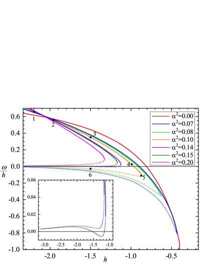
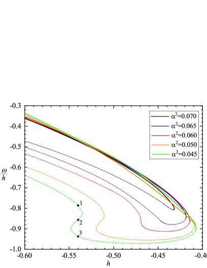
Figure 1: The scaled eigenvalue $\omega/h$ of the localized fermionic mode is shown versus the Yukawa coupling $h$ for several values of the effective coupling $\alpha^{2}$. The solid lines represent the Skyrmion branches, while the dotted lines correspond to the BM and deformed BM branches. Note that the positive continuum resides at $\omega/h=-1$, since $h<0$. a) The change of the spectral flow with increasing $\alpha^{2}$ is illustrated. The set of points 1 - 6 along the $\alpha^{2}=0.1$ branches represent illustrative configurations, whose matter and metric profile functions are shown in Fig. 2. The inset highlights the presence of multiple branches close to the transition of the bifurcation point from positive to negative eigenvalues $\omega$. b) The multibranch structure for small values of $\alpha$ is illustrated. The set of points 1 - 3 along the $\alpha^{2}=0.045$ branches (corresponding to Yukawa coupling $h=-0.54$) represents configurations, whose matter and metric profile functions are shown in Fig. 3.

Turning next to the presence of the fermions, we recall that in the limit of effective coupling $\alpha=0$ (taken in the limit of gravitational coupling $G=0$), the Skyrmion-fermion system features spectral flow in Minkowski spacetime [28, 29, 30]. This is illustrated by the red solid curve in Fig. 1a, where the fermion eigenvalue $\omega$, scaled by the Yukawa coupling $h$, is shown versus $h$ for several values of $\alpha$, starting from the Minkowski limit $\alpha=0$. In that case, the fermionic mode emerges from the positive continuum at a Yukawa coupling of $h_{\text{cr}}\approx-0.40$. Note that the positive continuum resides in the figure at $\omega/h=-1$, since the Yukawa coupling $h$ is negative.

As the Yukawa coupling decreases below $h_{\text{cr}}$, the eigenvalue $\omega$ decreases, i.e., the scaled eigenvalue $\omega/h$ increases. The eigenvalue $\omega$ then reaches zero at some particular value of the Yukawa coupling $h$. With the further decrease of $h$ the eigenvalue $\omega$ decreases further toward the negative continuum. Thus, we observe a single fermionic mode flowing monotonically from the positive to the negative continuum, in agreement with the index theorem.

In the absence of gravity, the only parameter affecting the profile function of the Skyrmion due to the backreacting fermion is the Yukawa coupling. The profile function always decreases monotonically from $F(0)=\pi$ to $F(\infty)=0$. However, the effective size of the configuration and the mass decrease as the magnitude of the coupling becomes stronger. While there are also other bound modes in the spectrum of the Dirac fermions localized on the Skyrmion in Minkowski spacetime [28, 29, 30], the normalizable bound mode crossing zero is unique.

Let us next include gravity and consider the dependence of the eigenvalue $\omega$ on the Yukawa coupling $h$ for a set of values of the effective coupling $\alpha$. One expects that instead of a single branch of Skyrmion-fermion solutions now two branches of solutions should arise. This expectation is due to the fact that for finite $\alpha$ the fermion may be localized and backreacting on the solutions of either the Skyrmion branch or of the BM branch.

As seen in Fig. 1, the presence of gravity indeed changes the picture accordingly and thus dramatically. The single zero crossing fermionic level present in Minkowski spacetime, that is related to the topology of the Skyrmion, thus undergoes a significant change as the Skyrmion-fermion system evolves toward the BM solution.

As the effective coupling $\alpha$ increases from zero, there arise indeed two branches of solutions, that we will refer to as well as Skyrmion and BM branches. We display these branches with different line styles in Fig. 1 and subsequent figures, showing the Skrymion branches with solid curves and the BM branches with dotted curves.

Now the fermionic mode no longer emerges from the positive continuum. But for each $\alpha$ there is a maximal value of the Yukawa coupling $h_{\text{max}}(\alpha)<h_{\text{cr}}$, where the branches of solutions arise. The fermionic eigenvalue $\omega$ at the bifurcation point of the branches decreases with decreasing $h$, passing zero at some point. Although the bifurcation point then resides at $\omega<0$ for larger values of $\alpha$, the eigenvalues still approach zero with decreasing $h$ along the BM branch.

In fact, the inset in Fig. 1a shows that in a small parameter range, the observed pattern is slightly more complicated. We do not only see the Skyrmion branch, obtained by varying $G$, and the BM branch, obtained by varying $f_{\pi}$, while $\alpha$ is the same on both branches. But there arises a small intermediate branch in the vicinity of the transition of the eigenvalue $\omega$ to purely negative values. This branch is also displayed with dotted line style, and in combination with the BM branch this will be referred to as a deformed BM branch.

We associate the reason for this subtlety with our considerations above, where we introduced the dimensionless Yukawa coupling $h\to h/(a_{0}f_{\pi})$. Hence, the same value of the coupling $h$ may correspond to different choices of all three parameters, and therefore one may expect multiple branches of solutions to appear. Since we fix the normalization condition in our numerical analysis to a particular value of the Skyrme parameter $a_{0}$, the branches of solutions may be related to the variation of the two remaining parameters, $h$ and $f_{\pi}$. In turn, variations of the latter parameter may be related to a corresponding change of the effective gravitational constant $\alpha$.

When we consider very small values of $\alpha$, where the eigenvalues of the Dirac operator get close to the positive continuum, this phenomenon of multiple branches is seen again, and is illustrated in Fig. 1b. Here a more detailed analysis of the critical behavior of the solutions reveals these interesting features, as $\alpha^{2}<0.06$. Then there is no longer a single bifurcation point, at which the Skyrmion and BM branches merge, but again multiple branches appear, deforming the BM branch. For example, for $\alpha^{2}=0.045$ there are three bifurcation points, as seen in Fig. 1b. The figure also shows that as $\alpha^{2}$ is increased above $0.06$ the multibranch pattern with several bifurcation points disappears and is replaced by a single bifurcation point with double branch structure.

III.2.2 Field configurations

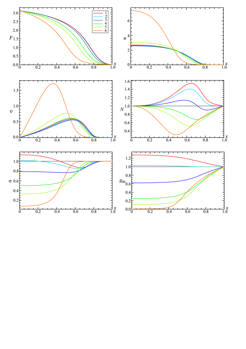
Figure 2: The profile functions $F$, $u$, $v$, $N$, and $\sigma$ of the gravitating Skyrmion-fermion system are shown versus the compactified radial coordinate $x$ for $\alpha^{2}=0.1$ for the points 1 - 6 in Fig. 1a. The solution labeled by point 2 corresponds to zero ADM mass.

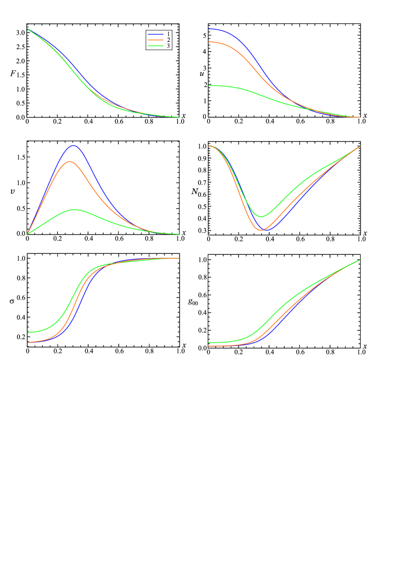
Figure 3: The profile functions $F$, $u$, $v$, $N$, and $\sigma$ of the gravitating Skyrmion-fermion system are shown versus the compactified radial coordinate $x$ for $\alpha^{2}=0.045$ for the points 1 - 3 in Fig. 1b.

In order to get a better understanding of the backreacting Skrymion-fermion systems and the associated spectral flow, let us now inspect some field configurations. We first consider the configurations labeled by points 1 - 6 in Fig. 1a. These points correspond to configurations with $\alpha^{2}=0.1$ and several values of the Yukawa coupling $h$. Points 1 - 4 reside on the Skyrmion branch, point 5 represents the configuration at the bifurcation of the branches, and point 6 resides on the BM branch.

We exhibit the respective sets of profile functions $F$, $u$, $v$, $N$, and $\sigma$ together with the metric component $g_{00}$ in Fig. 2. The configuration on the BM branch (point 6) possesses the smallest size. This is not unexpected, since the BM solution itself would shrink to a point in the present coordinate system. The fermion functions $u$ and $v$ then need to reach large values in the inner region to satisfy the normalization condition. Toward the bifurcation of the branches (point 5) the size of the configurations increases, and then continues to increase along the Skyrmion branch.

We further observe that as the fermion eigenvalue $\omega$ crosses zero (point 4) and then becomes negative, the metric functions $N(r)$ and $\sigma(r)$ possess increasing the minimal values. Interestingly, when $h$ is further decreased along the Skyrmion branch, the metric function $N(r)$ is no longer bounded by its asymptotic values from above. Instead, $N(r)$ increases above unity, first only in the inner part (point 3), and then everywhere in the interior (points 2 and 1), as seen in Fig. 2. Clearly, this has effects on the mass of the configurations, as discussed below.

We display in Fig. 3 the profile functions of the fields of the backreacting Skyrmion-fermion system for configurations in the multibranch region for small $\alpha$, close to the positive continuum. In particular, we show the three sets of functions obtained for $\alpha^{2}=0.045$ and $h=-0.54$, that are labeled as points 1 - 3 in Fig. 1b. The figure clearly shows that the solutions become increasingly localized, as we move to smaller fermion eigenvalues along the deformed BM branch. On the other hand, the ADM mass of these three solutions remains almost the same.

III.2.3 ADM mass

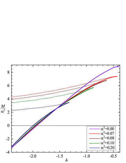
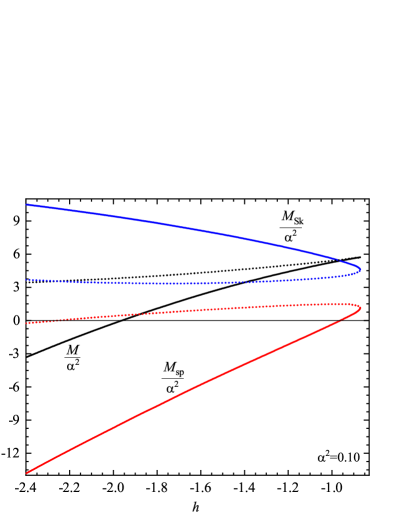
Figure 4: a) The scaled ADM mass $M/\alpha^{2}$ of the gravitating Skyrmion-fermion system is shown versus the Yukawa coupling $h$ for a set of values of the effective coupling $\alpha^{2}$. b) The contributions to the scaled total ADM mass ($M/\alpha^{2}$, black) from the fermion ($M_{\text{sp}}/\alpha^{2}$, red) and the Skyrme ($M_{\text{Sk}}/\alpha^{2}$, blue) fields are shown versus the Yukawa coupling $h$ for effective coupling $\alpha^{2}=0.1$.

We exhibit the ADM mass of the Skyrmion-fermion system in Fig. 4a, where we display the scaled mass $M/\alpha^{2}$ versus the Yukawa coupling $h$ for a set of values of the effective coupling $\alpha$, also shown in Fig. 1. The figure highlights again the bifurcations of the Skyrmion branches (solid) with the BM branches (dotted). As noted above, the maximal value of the Yukawa coupling is reached in the flat spacetime limit ($h\approx-0.4$), and decreases with increasing $\alpha$.

For a given value of the Yukawa coupling $h$, the ADM mass of the configurations on the Skyrmion branch is smaller than the mass on the BM branch. With increasing $\alpha$ the mass of the configurations on the BM branches, including the bifurcation points, decreases. In contrast, the mass on the lower parts of the Skyrmion branches does not vary significantly as $\alpha$ is increased.

Intriguingly, the ADM mass on the Skyrmion branches crosses zero when the Yukawa coupling is decreased, as demonstrated in Fig. 4. Inspection of the configurations at this critical point with $M=0$ shows that the metric component $g_{00}$ is nearly unity almost everywhere in space, and that the first derivative of the metric function $N$ at spatial infinity vanishes. This is illustrated in Fig. 2 by the functions corresponding to point 2.

Beyond this critical point, the ADM mass of the backreacting Skyrmion-fermion system becomes negative as the Yukawa coupling $h$ decreases along the Skyrmion branch, as seen in Fig. 4. While surprising at first, this hints at the capacity of fermions to violate the energy conditions. In contrast to this intriguing behavior of the ADM mass on the Skyrmion branch, the mass remains always positive along the BM branch.

To get further insight, let us compare the contributions of the Skyrmion and the fermion fields to the total mass. We present in Fig. 4b the dependence of the corresponding scaled quantities $M_{\text{Sk}}/\alpha^{2}$ and $M_{\text{sp}}/\alpha^{2}$ on the Yukawa coupling $h$ for $\alpha^{2}=0.10$, together with the scaled total mass $M/\alpha^{2}=(M_{\text{Sk}}+M_{\text{sp}})/\alpha^{2}$. These mass contributions are obtained by evaluating $M_{\text{Sk}}=\alpha^{2}\int dr\,r^{2}(T_{0}^{0})_{\text{Sk}}$ and $M_{\text{sp}}=\alpha^{2}\int dr\,r^{2}(T_{0}^{0})_{\text{sp}}$ (with $(T_{0}^{0})_{\text{Sk}}$ and $(T_{0}^{0})_{\text{sp}}$ given by Eqs. (35) and (38), respectively). Clearly, the negative contribution of the fermionic mode becomes dominant on the Skyrmion branch, rendering the total mass negative. On the BM branch, on the other hand, both contributions remain positive (for $h>-2.25$).

When we consider the scaled ADM mass $M/\alpha^{2}$ for configurations obtained by varying the effective coupling $\alpha$ for a set of fixed values of the Yukawa coupling $h$, we again observe two branches of solutions, a Skyrmion branch and a BM branch, that bifurcate at some maximal value $\alpha_{\text{max}}(h)$. As the Yukawa coupling $h$ decreases, $\alpha_{\text{max}}(h)$ increases. Curiously, at a particular value of the Yukawa coupling ($h=-1.565$) the scaled mass $M/\alpha^{2}$ remains approximately constant along the Skyrmion branch [63].

III.2.4 Violation of the null and weak energy conditions

We now demonstrate that the intriguing behavior of the solutions of the system (22) - (26) on the Skyrmion branches is related to the violation of the null and weak energy conditions. These demand that the stress-energy tensor $T_{\mu\nu}$ of the system satisfies the following inequalities,

$$T_{\mu\nu}k^{\mu}k^{\nu}\geq 0\quad\text{and}\quad T_{\mu\nu}V^{\mu}V^{\nu}\geq 0,$$

for any light-like vector $k^{\mu}$, $g_{\mu\nu}k^{\mu}k^{\nu}=0$, and for any timelike vector $V^{\mu}$, $g_{\mu\nu}V^{\mu}V^{\nu}>0$, respectively (for a review, see, e.g., Ref. [75]). For the system (1) and the spherically symmetric Ansatz (14) - (17), the only non-vanishing components of the stress-energy tensor (12) of the Skyrme field are

$$\left(T^{0}_{0}\right)_{\text{Sk}}= N\frac{2\sin^{2}F+r^{2}}{2r^{2}}{F^{\prime}}^{2}+\frac{\sin^{2}F+2r^{2}}{2r^{4}}\sin^{2}F,$$ (35)

$$\left(T^{1}_{1}\right)_{\text{Sk}}= -N\frac{2\sin^{2}F+r^{2}}{2r^{2}}{F^{\prime}}^{2}+\frac{\sin^{2}F+2r^{2}}{2r^{4}}\sin^{2}F,$$ (36)

$$\left(T^{2}_{2}\right)_{\text{Sk}}= \left(T^{3}_{3}\right)_{\text{Sk}}=\frac{1}{2}N{F^{\prime}}^{2}-\frac{\sin^{4}F}{2r^{4}},$$ (37)

and of the stress-energy tensor (13) of the fermion field are

$$\left(T^{0}_{0}\right)_{\text{sp}}= \omega\frac{u^{2}+v^{2}}{\sqrt{N}\sigma},$$ (38)

$$\left(T^{1}_{1}\right)_{\text{sp}}= 2uv\frac{hr\sin F+1}{r}+h\cos F\left(v^{2}-u^{2}\right)-\omega\frac{u^{2}+v^{2}}{\sqrt{N}\sigma},$$ (39)

$$\left(T^{2}_{2}\right)_{\text{sp}}= \left(T^{3}_{3}\right)_{\text{sp}}=-\frac{uv}{r}.$$ (40)

These components are given in terms of dimensionless quantities (following the rescaling $T^{\mu}_{\nu}\to T^{\mu}_{\nu}/(a_{0}^{2}f_{\pi}^{4})$). The null and the weak energy conditions for the backreacting Skyrmion-fermion system then become

$$\begin{split}\epsilon+p\equiv&T^{0}_{0}-T^{1}_{1}=N\frac{2\sin^{2}F+r^{2}}{r^{2}}{F^{\prime}}^{2}\\ &+h\left[\cos F\left(u^{2}-v^{2}\right)-2uv\sin F\right]+2\omega\frac{u^{2}+v^{2}}{\sqrt{N}\sigma}-\frac{2uv}{r}\geq 0,\end{split}$$ (41)

where $\epsilon$ denotes the energy density and $p$ the radial pressure. The weak energy condition also implies $\epsilon\equiv T_{0}^{0}\geq 0$.

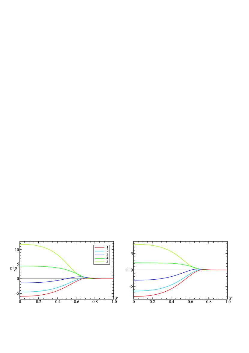
Figure 5: The validity, respectively violation, of the null and weak energy conditions is demonstrated for the Skyrmion-fermion solutions labeled by points 1 - 5 in Fig. 1a. a) The sum ($\epsilon+p$) of the energy density $\epsilon$ and the pressure $p$ is shown versus the compactified radial coordinate $x$. b) The energy density $\epsilon$ is shown for the same set of solutions.

Evidently, the first term on the right-hand side of the expression (41) is related to the contribution of the Skyrme field. It is always positive, and a violation of the null/weak energy conditions can only be related to the contribution of the Dirac field.

We display in Fig. 5a the combination $(\epsilon+p)$ on the right-hand side of the null/weak energy conditions (41) and in Fig. 5b the energy density $\epsilon$ versus the compactified radial coordinate $x$ for a set of Skyrmion-fermion solutions. In particular, we choose again the configurations considered earlier in detail, that are labeled by the points 1 - 5 in Fig. 1a for $\alpha^{2}=0.1$. Whereas the configurations at the bifurcation (point 5) and slightly further on the Skyrmion branch (point 4) still respect the energy conditions, these become violated as we progress along the Skyrmion branch (points 3, 2, and 1). We also note that for all configurations 1 - 5 the pressure $p$ is always positive and the violation of the null/weak energy conditions is only caused by the energy density.

III.2.5 Localized fermions with finite bare mass

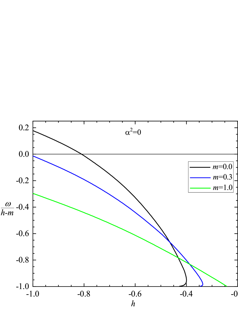
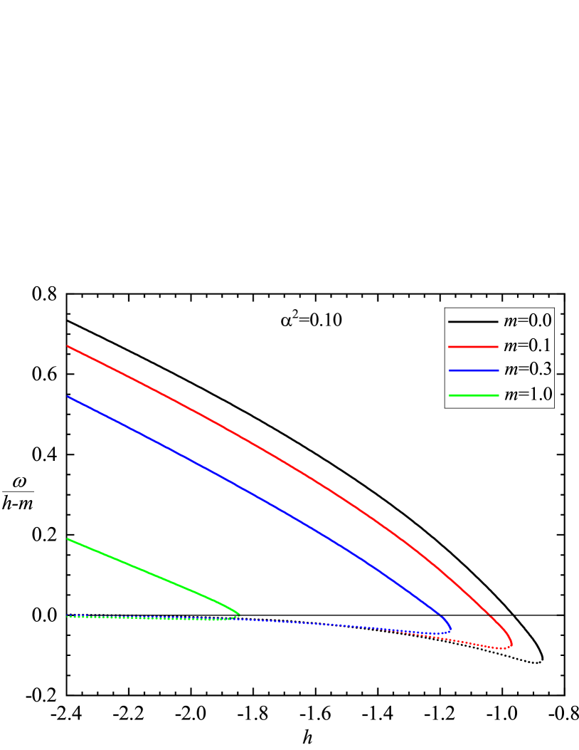
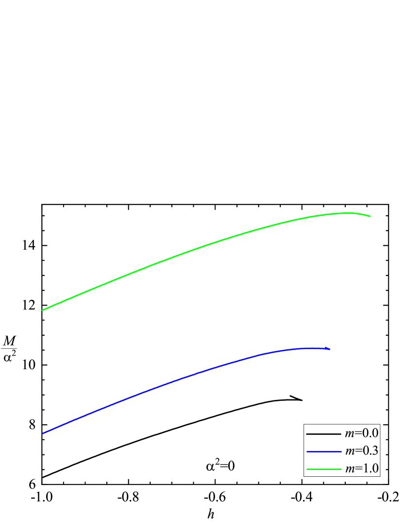
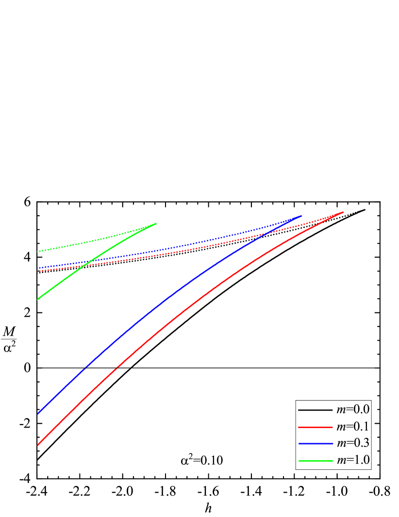
Figure 6: The influence of a finite bare mass $m$ of the fermions on the backreacting Skyrmion-fermion system is demonstrated. a) The scaled eigenvalue $\omega/(h-m)$ of the localized fermionic mode is shown versus the Yukawa coupling $h$ for several values of the bare mass $m$ in Minkowski space ($\alpha^{2}=0$), and b) for effective coupling $\alpha^{2}=0.10$. c) The scaled ADM mass $M/\alpha^{2}$ is shown versus the Yukawa coupling $h$ for several values of the bare mass $m$ in Minkowski space ($\alpha^{2}=0$), and d) for effective coupling $\alpha^{2}=0.10$. The solid lines represent the Skyrmion branches, while the dotted lines correspond to the BM branches.

We now address the influence of a finite value of the bare mass $m$ of the fermions on the Skyrmion-fermion configurations with backreaction taken into account. In particular, we consider several values of the bare mass $m$ for the system in Minkowski space and in the presence of gravity, and we exhibit our main findings in Fig. 6.

We note that the previously obtained pattern changes only slightly when massive fermionic modes are localized on the gravitating Skyrmion, and the Yukawa coupling $h$ and the effective coupling $\alpha$ are varied. First, we note that the asymptotic behavior of the fermion field is still given by Eq. (29) up to the replacement $h\to\bar{h}\equiv(h-m)$. The latter is necessary since the fermion obtains an effective mass $m_{\text{eff}}=m-h$ due to the Yukawa coupling. Consequently, the emergence of the fermionic mode from the positive continuum arises at $\omega/m_{\text{eff}}=1$ or, as shown in Fig. 6a, at $\omega/(h-m)=-1$.

Starting the discussion in Minkowski space ($\alpha^{2}=0$), we exhibit the scaled eigenvalue $\omega/(h-m)$ of the fermionic mode versus the Yukawa coupling $h$ in Fig. 6a for several values of the bare mass $m$, including the vanishing bare mass case for comparison. Clearly, the spectral flow exhibits the expected zero crossing behavior of the eigenvalue also for massive fermions, as the Yukawa coupling decreases.

However, as the bare mass increases from zero, also a new feature is observed. We note that for vanishing bare mass the scaled eigenvalue $\omega/h$ of the fermionic mode emerges from the positive continuum slightly below $h_{\text{max}}$. Thus the dependence of the scaled eigenvalue $\omega/h$ on the Yukawa coupling $h$ is not quite monotonic close to the positive continuum. With increasing bare mass this non-monotonic behavior of $\omega/(h-m)$ is reduced and then disappears, as seen in the figure for $m=0.3$ and $m=1.0$, respectively. We also observe in Fig. 6a that the critical value of the Yukawa coupling, where the localized mode emerges from the continuum, increases with increasing $m$.

In the presence of gravity two branches of solutions arise also for finite values of the fermion bare mass, the Skyrmion branch and the BM branch. This is illustrated in Fig. 6b for effective coupling $\alpha^{2}=0.10$. We observe that, with increasing $m$, the bifurcation point of the branches now arise at decreasing values of the Yukawa coupling $h$. Thus solutions for the backreacting Skyrmion-fermion system exist only for decreasing $h_{\text{max}}(m)$.

Next, we exhibit the scaled mass $M/\alpha^{2}$ versus the Yukawa coupling $h$ for these sets of solutions in Fig. 6c for Minkowski space and in Fig. 6d in the presence of gravity ($\alpha^{2}=0.10$). We note that in Minkowski space the scaled ADM mass of the configurations increases significantly with increasing bare mass, including the maximal value of the scaled ADM mass.

In contrast, when gravity is coupled to the system, the maximal value of the ADM mass depends only weakly on the bare mass $m$. Overall, the ADM mass retains its characteristic behavior discussed above, with the branches shifting toward smaller values of the Yukawa coupling $h$ with increasing bare mass. Along the Skyrmion branch the mass always crosses zero and then turns negative. Again, the energy conditions become violated along the Skyrmion branch for sufficiently small values of $h$.

III.2.6 Radially excited fermionic modes

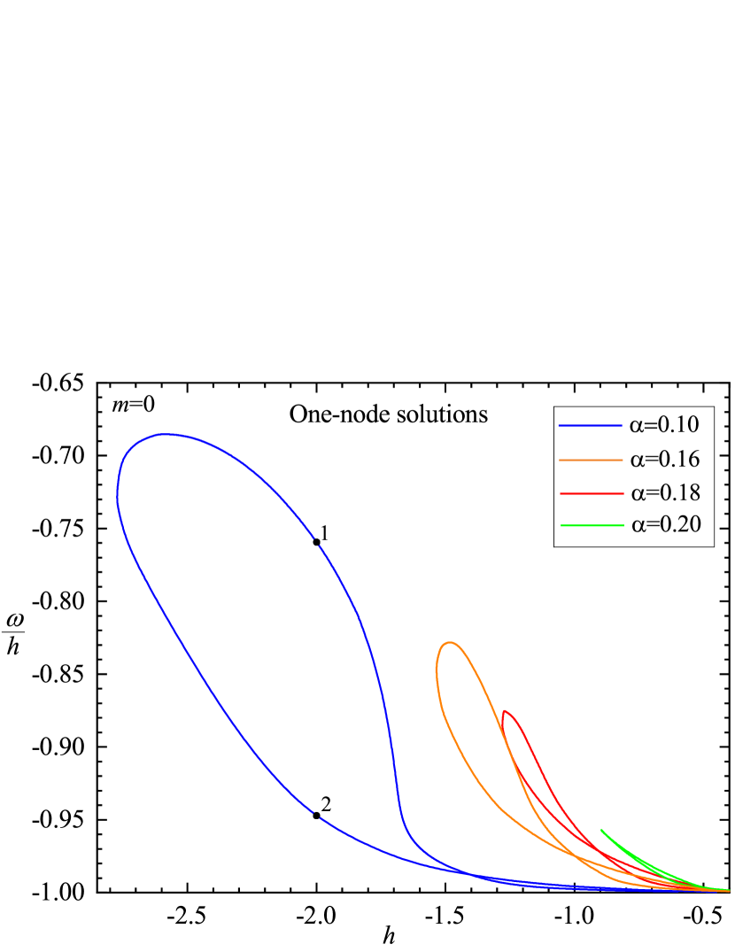
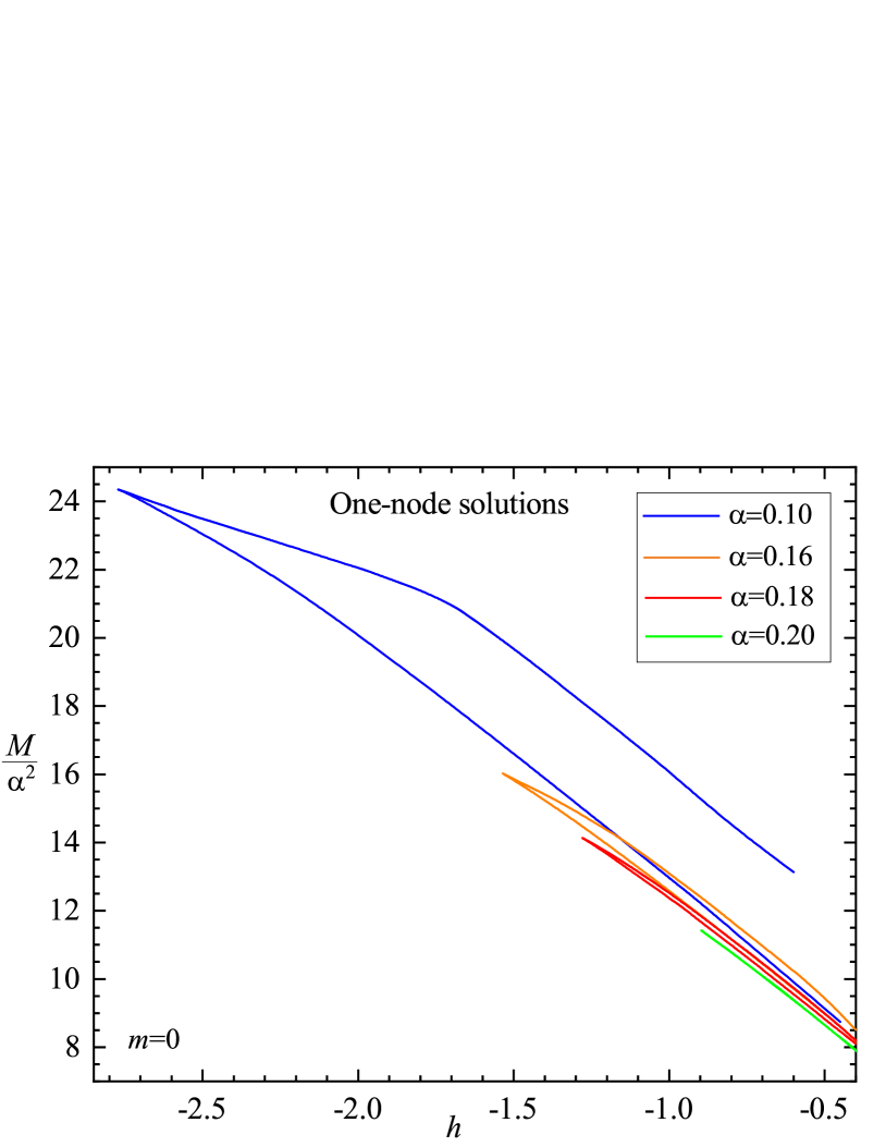
Figure 7: Spherically symmetric radially excited solutions are exhibited for several values of the effective coupling $\alpha^{2}$. a) The scaled eigenvalue $\omega/h$ of the localized fermionic mode is shown versus the Yukawa coupling $h$. Note that the positive continuum resides at $\omega/h=-1$. The points 1 and 2 on the $\alpha=0.1$ loop at $h=-2$ represent configurations, whose matter and metric profile functions are shown in Fig. 8. b) The scaled ADM mass $M/\alpha^{2}$ is shown versus the Yukawa coupling $h$.

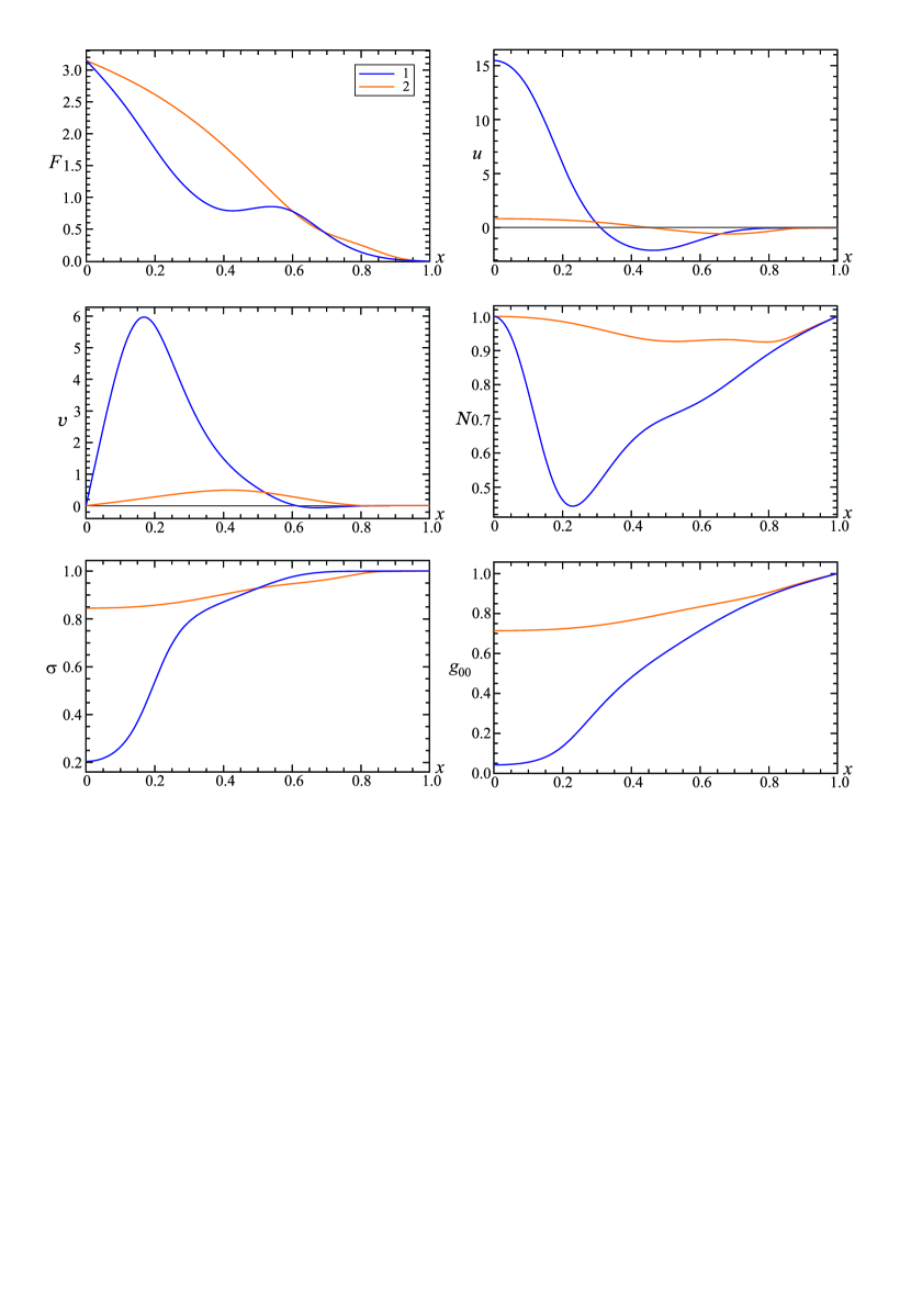
Figure 8: The profile functions $F$, $u$, $v$, $N$, and $\sigma$ of the radially excited solutions are shown versus the compactified radial coordinate $x$ for the points 1 and 2 on the $\alpha=0.1$ loop in Fig. 7.

So far we here addressed only the fundamental spherically symmetric gravitating Skyrmion-fermion solutions which have monotonic matter field functions $F(r)$, $u(r)$, and $v(r)$. However, we find in addition discrete families of radially excited solutions that feature an increasing number of zeros of their fermion functions. The corresponding spectral flow of these radially excited solutions is rather different from the spectral flow of the nodeless solutions discussed above.

As a particular example, we now consider configurations with one node of the fermion functions $u$ and $v$ each, and a nodeless Skyrmion profile function, restricting again to the case of vanishing bare mass, $m=0$. We display in Fig. 7 the scaled spectral flow for these radially excited solutions for several values of the effective coupling $\alpha$. Note that in contrast to the figures of the nodeless solutions, where $\alpha^{2}$ was specified, here $\alpha$ is shown in the legend.

Figure 7a exhibits the scaled eigenvalue $\omega/h$ versus the Yukawa coupling $h$, while Fig. 7b shows the scaled ADM mass $M/\alpha^{2}$ versus $h$. For small effective gravitational coupling $\alpha$, $\alpha^{2}\leq 0.04$, two branches of solutions emerge from the positive continuum at some critical value of the Yukawa coupling $h_{\text{cr}}<0$. Interestingly, this value is close to the critical value $h_{\text{max}}$, where the nodeless solutions emerge from the positive continuum in Minkowski space (see Fig. 1).

As seen in Fig. 7a, the scaled eigenvalue $\omega/h$ of the localized fermionic mode forms a typical double loop curve consisting of two crossing branches, when considered versus the Yukawa coupling $h$. By analogy with our consideration above, we may possibly identify the evolution of the configuration along one of these branches as related to the decrease of the Yukawa coupling, while the evolution along the second branch might be considered as being obtained by decreasing the Skyrme parameter $f_{\pi}$.

To obtain a better understanding of this branch structure, we consider two sets of solutions, labeled by points 1 and 2 in Fig. 7a. We show their profile functions $F$, $u$, $v$, $N$, and $\sigma$ versus the compactified radial coordinate $x$ in Fig. 8. The solution with its fermionic mode closer to the positive continuum (point 2) is weakly localized. The backreaction of this mode on the Skyrme field is small, and the metric functions are not far from the flat space limit. On the contrary, the solution on the second branch (point 1) is strongly localized, the backreaction of the fermionic mode is very significant, and the gravitational interaction is strong.

Addressing now the associated ADM mass of these radially excited solutions, the branch structure becomes more evident. As seen in Fig. 7b, both branches bifurcate at a maximal value of the scaled ADM mass $M/\alpha^{2}$, that corresponds to a minimal value of the Yukawa coupling $h$. With increasing effective coupling $\alpha$, the maximal value of the scaled ADM mass decreases, while the minimal value of the Yukawa coupling increases. In fact, the solutions with one node rapidly degenerate, as the coupling to gravity becomes stronger, and they cease to exist as $\alpha^{2}>0.04$. We note that we do not observe bifurcations between the solutions with one node and the nodeless configurations.

Most importantly, we note that none of the solutions with one node exhibit a zero mode. The double loop formed by the scaled eigenvalues $\omega/h$ never crosses zero, but remains always negative. Consequently, their ADM mass neither becomes zero or turns negative. Those intriguing effects are only observed for the fundamental (nodeless) solutions.

IV Conclusions

Here we have considered gravitating solutions of Einstein-Skyrme-Dirac theory. The bosonic sector of this theory gives rise to localized solutions, connected to the Skyrmions in flat space and to the Bartnik-McKinnon solutions of Einstein-Yang-Mills theory. In the presence of gravity these globally regular solutions spawn hairy black hole solutions in General Relativity [14, 15, 16, 17, 18, 19].

Since Skyrmions are topological solitons, the index theorem guarantees the occurrence of the spectral flow of a normalizable fermionic mode bound to them. In Minkowski space the backreaction of a spin-isospin singlet fermionic mode on the spherically symmetric Skyrmion with unit topological charge was studied already long ago [28, 29, 30]. Depending on the Yukawa coupling strength, this mode emerges from the positive continuum, crosses zero and evolves toward the negative continuum.

Here we have presented a detailed study of the generalization of this phenomenon by minimally coupling the matter fields to gravity [63]. When gravity is added, we basically observe two branches of localized solutions, the Skyrmion branch and the BM branch, as the Yukawa coupling strength is varied, instead of the single branch present in Minkowski space. The two branches then emerge at a bifurcation point, that is not connected to the positive continuum.

For small gravitational coupling the branches still emerge at bifurcation points with positive eigenvalue of the fermionic mode, and then evolve toward smaller eigenvalues, with the modes on the Skyrmion branch evolving toward the negative continuum. For larger gravitational coupling the spectral flow features merely negative eigenvalues of the fermionic mode. Taking into account the backreaction of the fermionic mode on the gravitating bosonic configurations thus implies dramatic consequences: The ADM mass of the Skyrmion-fermion systems crosses zero along the Skyrmion branches and then turns negative. As one may expect, this is associated with the violation of the energy conditions.

While we have mostly considered the backreacting Skyrmion-fermion systems for vanishing bare mass of the fermions, we have also shown that the presence of a finite fermionic bare mass does not alter the basic scenario of the evolution of the spectral flow significantly. In contrast, when we consider instead of the fundamental singlet mode a radially excited state, the spectral flow changes drastically: neither zero modes nor negative ADM masses arise.

It may be of interest to compare with another well-known system, the self-gravitating non-Abelian monopole [11, 12, 13]. In both cases the flat space configurations represent spherically symmetric topological solitons in (3+1)-dimensions, and there is a spin-isospin singlet fermionic mode localized on the soliton.

However, the pattern of the dynamical evolution of the gravitating monopole and of the Skyrmion is different. While the gravitating monopole solutions bifurcate with an extremal Reissner-Nordström black hole, the gravitating Skyrmions bifurcate with a second branch of solutions, tending to the regular scaled BM solution. Moreover, the eigenvalue of the Dirac operator of the fermionic mode localized on the monopole is always zero. It does not depend on the strength of the Yukawa coupling. This mode is fully absorbed into the interior of the black hole as the configuration approaches the Reissner-Nordström limit [51].

We note that the possibility of the emergence of a negative mass in General Relativity is being discussed since a long time [76, 77] (for some recent work, see, e.g., Refs. [78, 79, 80]). It has also been pointed out that a region of negative energy density may collapse to a black hole with an unusual topology of the event horizon [81]. One might therefore wonder whether, in the case of Skyrmion-fermion systems with negative mass, the possibility of forming a black hole of negative mass carrying Skyrmion-fermion hair might arise. This would be of particular interest, since previous attempts to obtain black holes with fermion hair in (3+1)-dimensional asymptotically flat spacetime have failed [52, 53, 56, 82].

Finally, we would like to remark that it was suggested that Skyrmions might have technological significance in the future, providing fuel for the engines of Star Trek starships [83]. Our present results indicate that Skyrmions might even have far wider implications, providing examples of anti-gravitating matter.

References

- [1] G. ’t Hooft, Nucl. Phys. B 79, 276 (1974).
- [2] A. M. Polyakov, JETP Lett. 20, 194 (1974).
- [3] T. H. R. Skyrme, Proc. Roy. Soc. Lond. A 260, 127 (1961).
- [4] T. H. R. Skyrme, Nucl. Phys. 31, 556 (1962).
- [5] L. D. Faddeev, Print-75-0570 (IAS, PRINCETON).
- [6] L. D. Faddeev and A. J. Niemi, Nature 387, 58 (1997).
- [7] N. S. Manton and P. Sutcliffe, Topological solitons (Cambridge University Press, 2004).
- [8] Y. M. Shnir, Topological and Non-Topological Solitons in Scalar Field Theories (Cambridge University Press, 2018).
- [9] M. S. Volkov and D. V. Gal’tsov, Phys. Rept. 319, 1 (1999).
- [10] M. S. Volkov, “Hairy black holes in the XX-th and XXI-st centuries”, Proceedings of the Fourteenth Marcel Grossmann Meeting, eds M. Bianchi, R. Jantzen and R. Ruffini, World Scientific, pp. 1779-1798 (2017).
- [11] K. M. Lee, V. P. Nair, and E. J. Weinberg, Phys. Rev. D 45, 2751 (1992).
- [12] P. Breitenlohner, P. Forgacs, and D. Maison, Nucl. Phys. B 383, 357 (1992).
- [13] P. Breitenlohner, P. Forgacs, and D. Maison, Nucl. Phys. B 442, 126 (1995).
- [14] H. Luckock and I. Moss, Phys. Lett. B 176, 341 (1986).
- [15] N. K. Glendenning, T. Kodama, and F. R. Klinkhamer, Phys. Rev. D 38, 3226 (1988).
- [16] S. Droz, M. Heusler, and N. Straumann, Phys. Lett. B 268, 371 (1991).
- [17] M. Heusler, S. Droz, and N. Straumann, Phys. Lett. B 271, 61 (1991).
- [18] P. Bizon and T. Chmaj, Phys. Lett. B 297, 55 (1992).
- [19] M. Heusler, N. Straumann, and Z. h. Zhou, Helv. Phys. Acta 66, 614 (1993).
- [20] M. F. Atiyah, V. K. Patodi, and I. M. Singer, Math. Proc. Cambridge Phil. Soc. 77, 43 (1975).
- [21] C. Caroli, P.G. de Gennes, and J. Matricon, Phys. Lett.9, 307 (1964).
- [22] R. Jackiw and C. Rebbi, Phys. Rev. D 13, 3398 (1976).
- [23] R. F. Dashen, B. Hasslacher, and A. Neveu, Phys. Rev. D 10, 4130 (1974).
- [24] Y. Z. Chu and T. Vachaspati, Phys. Rev. D 77, 025006 (2008).
- [25] C. R. Nohl, Phys. Rev. D 12, 1840 (1975).
- [26] J. Boguta and J. Kunz, Phys. Lett. B 154, 407 (1985).
- [27] C. J. Callias, Phys. Rev. D 16, 3068 (1977).
- [28] J. R. Hiller and T. F. Jordan, Phys. Rev. D 34, 1176 (1986).
- [29] S. Kahana and G. Ripka, Nucl. Phys. A 429, 462 (1984).
- [30] A. P. Balachandran and S. Vaidya, Int. J. Mod. Phys. A 14, 445 (1999).
- [31] D. Stojkovic, Phys. Rev. D 63, 025010 (2001).
- [32] R. Jackiw and P. Rossi, Nucl. Phys. B 190, 681 (1981).
- [33] V. A. Rubakov, Nucl. Phys. B 203, 311 (1982).
- [34] C. G. Callan, Jr., Phys. Rev. D 26, 2058 (1982).
- [35] E. Witten, Nucl. Phys. B 249, 557 (1985).
- [36] V. A. Gani, V. G. Ksenzov, and A. E. Kudryavtsev, Phys. Atom. Nucl. 73, 1889 (2010).
- [37] A. Amado and A. Mohammadi, Eur. Phys. J. C 77, 465 (2017).
- [38] V. Klimashonok, I. Perapechka, and Y. Shnir, Phys. Rev. D 100, 105003 (2019).
- [39] I. Perapechka, N. Sawado, and Y. Shnir, JHEP 10, 081 (2018).
- [40] Y. Amari, N. Sawado, and S. Yamamoto, JHEP 06 (2024), 057
- [41] I. Perapechka and Y. Shnir, Phys. Rev. D 99, 125001 (2019).
- [42] I. Perapechka and Y. Shnir, Phys. Rev. D 101, 021701 (2020).
- [43] J. G. F. Campos and A. Mohammadi, JHEP 08, 180 (2022).
- [44] V. A. Gani, A. Gorina, I. Perapechka, and Y. Shnir, Eur. Phys. J. C 82, 757 (2022).
- [45] D. Bazeia, J. G. F. Campos, and A. Mohammadi, JHEP 12, 085 (2022).
- [46] D. Saadatmand and H. Weigel, Phys. Rev. D 107, 036006 (2023).
- [47] H. Weigel and D. Saadatmand, Universe 10, 13 (2024).
- [48] A. H. Taub, Phys. Rev. 51, 512 (1937).
- [49] M. S. Volkov, Phys. Lett. B 334, 40 (1994).
- [50] J. Kunz and Y. Brihaye, Phys. Lett. B 304, 141 (1993)
- [51] V. Dzhunushaliev, V. Folomeev, and Y. Shnir, Phys. Rev. D 108, 065005 (2023).
- [52] F. Finster, J. Smoller, and S. T. Yau, Phys. Rev. D 59, 104020 (1999).
- [53] C. Herdeiro, I. Perapechka, E. Radu, and Y. Shnir, Phys. Lett. B 797, 134845 (2019).
- [54] V. Dzhunushaliev and V. Folomeev, Phys. Rev. D 99, 084030 (2019).
- [55] V. Dzhunushaliev and V. Folomeev, Phys. Rev. D 99, 104066 (2019).
- [56] C. Herdeiro, I. Perapechka, E. Radu, and Y. Shnir, Phys. Lett. B 824, 136811 (2022).
- [57] J. L. Blázquez-Salcedo and C. Knoll, Eur. Phys. J. C 80, 174 (2020).
- [58] J. L. Blázquez-Salcedo, C. Knoll, and E. Radu, Phys. Rev. Lett. 126, 101102 (2021).
- [59] S. Bolokhov, K. Bronnikov, S. Krasnikov, and M. Skvortsova, Grav. Cosmol. 27, 401 (2021).
- [60] R. A. Konoplya and A. Zhidenko, Phys. Rev. Lett. 128, 091104 (2022).
- [61] C. Armendariz-Picon and P. B. Greene, Gen. Rel. Grav. 35, 1637 (2003).
- [62] Y. F. Cai and J. Wang, Class. Quant. Grav. 25, 165014 (2008).
- [63] V. Dzhunushaliev, V. Folomeev, J. Kunz, and Y. Shnir, Phys. Lett. B 855, 138812 (2024).
- [64] R. Bartnik and J. Mckinnon, Phys. Rev. Lett. 61, 141 (1988).
- [65] S. R. Dolan and D. Dempsey, Class. Quant. Grav. 32, 184001 (2015).
- [66] T. Eguchi, P. B. Gilkey, and A. J. Hanson, Phys. Rept. 66, 213 (1980).
- [67] M. Gell-Mann and M. Levy, Nuovo Cim. 16, 705 (1960).
- [68] S. Krusch, J. Phys. A 36, 8141 (2003).
- [69] Y. Shnir, Phys. Scripta 67, 361 (2003).
- [70] R. Jackiw and C. Rebbi, Phys. Rev. Lett. 36, 1116 (1976).
- [71] G. S. Adkins, C. R. Nappi, and E. Witten, Nucl. Phys. B 228, 552 (1983).
- [72] N. S. Manton and S. W. Wood, Phys. Rev. D 74, 125017 (2006).
-
[73]
N.I.M. Gould, J.A. Scott, Y. Hu,
ACM Trans. Math. Softw. 33, 10 (2007);
O. Schenk, K. Gartner, Future Gener. Comput. Syst. 20, 475 (2004). - [74] J. Kunz, I. Perapechka, and Y. Shnir, JHEP 07, 109 (2019).
- [75] V. A. Rubakov, Phys. Usp. 57, 128 (2014).
- [76] H. Bondi, Rev. Mod. Phys. 29, 423 (1957).
- [77] D. Harari and C. Lousto, Phys. Rev. D 42, 2626 (1990).
- [78] S. Mbarek and M. B. Paranjape, Phys. Rev. D 90, 101502 (2014).
- [79] J. S. Farnes, Astron. Astrophys. 620, A92 (2018).
- [80] C. H. Hao, L. X. Huang, X. Su, and Y. Q. Wang, [arXiv:2312.03800 [gr-qc]].
- [81] R. B. Mann, Class. Quant. Grav. 14, 2927 (1997).
- [82] J. l. Jing, Phys. Rev. D 70, 065004 (2004).
- [83] S. Krusch and P. Sutcliffe, J. Phys. A 37, 9037 (2004).