Universal Approximation Theory: The basic theory for deep learning-based computer vision models

Abstract

Computer vision (CV) is one of the most crucial fields in artificial intelligence. In recent years, a variety of deep learning models based on convolutional neural networks (CNNs) and Transformers have been designed to tackle diverse problems in CV. These algorithms have found practical applications in areas such as robotics and facial recognition. Despite the increasing power of current CV models, several fundamental questions remain unresolved: Why do CNNs require deep layers? What ensures the generalization ability of CNNs? Why do residual-based networks outperform fully convolutional networks like VGG? What is the fundamental difference between residual-based CNNs and Transformer-based networks? Why can CNNs utilize LoRA and pruning techniques? The root cause of these questions lies in the lack of a robust theoretical foundation for deep learning models in CV. To address these critical issues and techniques, we employ the Universal Approximation Theorem (UAT) to provide a theoretical basis for convolution- and Transformer-based models in CV. By doing so, we aim to elucidate these questions from a theoretical perspective.

1 Introduction

As a core branch of artificial intelligence, CV has a wide range of applications, encompassing tasks such as image segmentation (Minaee et al. 2021; Wang et al. 2022a), classification (Rawat and Wang 2017; Wang et al. 2017), video synthesis (Wang et al. 2018, 2019a), and restoration (Wang et al. 2019b; Nah et al. 2019). This broad applicability highlights its enormous technical potential and practical significance, making the intelligent processing of CV tasks a highly important area of research. The most effective solutions in this field today are based on deep learning algorithms.

One of the earliest and most influential works in using deep learning for CV was LeNet (Lecun et al. 1998), which pioneered the use of CNNs for handwritten digit recognition, ushering in a new era of image processing. Following this, AlexNet’s (Krizhevsky, Sutskever, and Hinton 2017) remarkable performance on the ImageNet (Russakovsky et al. 2014) dataset not only achieved a significant leap in image classification accuracy but also cemented CNNs as the dominant method in visual processing. The subsequent introduction of ResNet (He et al. 2016) further improved image recognition accuracy and established residual-based structure as a foundational architecture for future network designs, influencing nearly all subsequent deep learning models (Ren et al. 2015; Xie et al. 2016; Szegedy et al. 2014; Gao et al. 2019; Liu et al. 2021).

In recent years, the success of Transformers (Vaswani et al. 2017) in the field of natural language processing (NLP) has gradually permeated CV. Researchers have begun designing models for CV based on Transformers, such as the Vision Transformer (ViT) (Dosovitskiy et al. 2020), Swin Transformer (Liu et al. 2021) and StructViT (Kim et al. 2024), which have demonstrated capabilities comparable to CNNs in image tasks (For convenience, we collectively refer to all Transformer-based models in the CV domain as ViTs.). Currently, research in deep learning for image processing predominantly revolves around CNNs (Huang et al. 2023; Wang et al. 2022b), Transformers (Shi 2023; Wang et al. 2023), or strategies that integrate both (Lv et al. 2023; Hou et al. 2024), continuously driving technological advancements.

Despite significant progress in deep learning-based CV, achieving performance that surpasses human capabilities in some areas, several questions remain unanswered. For example, what necessitates deep layers in CNNs? What underpins the generalization ability of CNNs? Why do residual-based networks surpass fully convolutional networks like VGG (Simonyan and Zisserman 2014) in performance? What are the core differences between residual-based CNNs and Transformer-based networks? We believe that the fundamental reason lies in the absence of a basic theory for CNNs. Although some researchers have attempted to explain CNNs through various methods, such as visualization techniques to analyze the relationship between feature maps and original images (Wei et al. 2016) and exploring CNNs from the frequency domain perspective (Yin et al. 2019; Xu, Zhang, and Xiao 2019), these explanations often have limitations and subjectivity. Similarly, studies on the interpretability of ViTs (Park and Kim 2022; Bai et al. 2022) suggest that MHA tend to capture low-frequency information, contrasting with the high-pass filtering nature of CNNs. These studies advocate for combining the strengths of both or improving ViTs to better understand high-frequency details.

However, these methods provide only intuitive visual explanations for specific issues and fail to offer a theoretical explanation for the widespread problems in CNNs and ViTs. Essentially, they describe or understand phenomena within CNNs or ViTs rather than presenting a complete theory for these architectures. To address these questions, we propose unifying CNNs and ViTs under the framework of the UAT by referencing the methods introduced in the UAT2LLMs (Wang and Li 2024). Using this framework, we aim to solve the aforementioned problems. Our contributions are as follows:

• We used the Matrix-Vector Method to demonstrate that the multi-layer convolutional and Transformer structures commonly employed in the field of CV are specific implementations of the UAT.

• We explained why CNNs require deep networks, considering the characteristics of image data and the UAT model perspective.

• We proved why the widely used residual structure in CV is so powerful.

• We compared multi-layer convolutional residual structures and Transformer structures from the UAT perspective, illustrating the source of their powerful capabilities and explaining why both models appear to have similar performance.

• we provided an explanation for LoRA and pruning in the context of CV.

The structure of this paper is as follows: In Section 2, we introduce the UAT and the Matrix-Vector Method, as well as their relationship. In Section 3, we use the Matrix-Vector Method to transform some commonly used operations in CV into matrix-vector forms, such as 2D convolution (3.1), 3D convolution (3.2), mean-pooling (3.3), and Transformers (3.4). In Section 4, we address some fundamental questions in CV: why CNN networks need to be deep (4.1), why residual-based CNNs are more powerful than VGG (4.2), the differences between residual-based CNNs and Transformer-based networks (4.3), and the theoretical support behind LoRA and pruning operations in CV (4.4).

2 UAT for CV

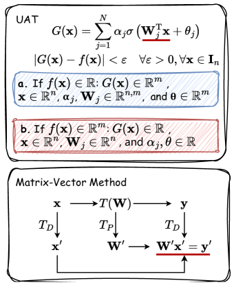
Figure 1: The basic format of UAT and The Matrix-Vector Method and their relationship.

We have previously introduced our goal of unifying CNNs and ViTs in the field of CV under the framework of UAT. Using UAT, we aim to explain existing problems in CV. So we will follow the UAT2LLMs’ (Wang and Li 2024) thoughts to leverage the Matrix-Vector Method proposed in UAT2LLMs to unify CNNs and ViTs under the UAT framework. Before formally unifying CNNs and ViTs within UAT, we will briefly introduce the Matrix-Vector Method and the unification approach proposed in UAT2LLMs.

Figure 1 simply outlines the proof route in UAT2LLMs: first, $G(\mathbf{x})$ represents the general form of UAT, capable of approximating Borel measurable functions within a closed interval(Cybenko 2007; Hornik, Stinchcombe, and White 1989), where $\mathbf{I}_{n}$ denotes an n-dimensional unit cube. UAT includes one-dimensional and high-dimensional approximations, corresponding to Figures 1.a and 1.b, respectively. It is evident that the basic UAT computing units $\mathbf{W}_{j}^{\mathrm{T}}\mathbf{x}+\theta_{j}$ corresponding to convolution, mean pooling, multi-head attention (MHA), and feed-forward networks (FFN) in CNNs and ViTs. Therefore, if we can transform these operations into matrix multiplication using the Matrix-Vector Method in Figures 1 (Details could be seen in UAT2LLMs), it becomes straightforward to prove that multi-layer CNNs and ViTs are specific implementations of UAT.

The Matrix-Vector Method is illustrated in Figure 1, where $T$ denotes various transformations in CNNs and ViTs, and $T_{D}$ and $T_{P}$ represent specific transformation methods. These transformations convert the input data $\mathbf{x}$ and output data $\mathbf{y}$, along with parameters $\mathbf{W}$, into vectors $\mathbf{x}^{\prime}$ and $\mathbf{y}^{\prime}$, and parameter matrices $\mathbf{W}^{\prime}$, satisfying the computational requirements shown in the Figure 1. To distinguish from the original variables, we will add a ^′ symbol to the upper right of the original variables, indicating their corresponding matrix-vector form. (Note: The key challenge is converting them into matrix-vector form, so bias terms are omitted here.) This approach also has the advantage of converting various transformations into a uniform matrix-vector form, allowing the entire network process to be expressed concisely using addition, multiplication, matrix operations, and activation functions, making it easier to compare models’ differences.

Additionally, due to the complexity of convolution and Transformer calculations, a computational tool called diamond matrix multiplication has been designed to clearly elucidate the process of converting convolution or Transformer operations into their corresponding matrix-vector representations. Its relationship with standard matrix multiplication is $\mathbf{W}\diamond\mathbf{x}=\mathbf{W}^{T}\mathbf{x}$. The diamond matrix enhances the clarity of this conversion process. The details and properties can be found in UAT2LLMs.

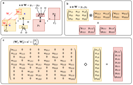
Figure 2: 1-O Conv2D process and the matrix-vector transformation example. In a, we present the general representation of a 1-O Conv2D operation. At the top, we provide the mathematical formula corresponding to the diagram. This approach is consistent in b and c as well. In the figure, we use $C_{I}$, $C_{O}$, $H$, and $W$ to denote the dimension name conventions for the input, convolution kernel, and output, as well as the elements within them. Additionally, we group the variables in the figure, such as $\mathbf{W}=Concat(\mathbf{W}_{1},\cdots,\mathbf{W}_{O})$. In b, we provide an example corresponding to a, and in c, we show the matrix-vector form of the example given in b. The following figures follow the same conventions.

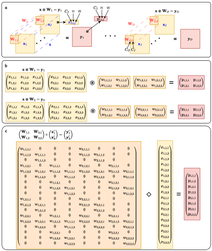
Figure 3: I-O Conv2D process and the matrix-vector transformation example.

3 The Matrix-Vector Method for CNNs and ViTs

In the previous sections, we explained that to unify CNNs and ViTs under the UAT, it is necessary to demonstrate that their various transformations (convolution, mean pooling, MHA, FFN) can be represented in matrix-vector form. UAT2LLMs has already shown how to represent MHA and FFN in matrix-vector form. Therefore, in this section, we will specifically demonstrate how to convert convolution and mean pooling in CNNs into matrix-vector form using the Matrix-Vector Method. Additionally, we will interpret the unique aspects of MHA in ViTs within the context of CV.

Considering that convolution in CV can be either 2D or 3D and that the input and output may consist of single or multiple channels. We use the notation 1 to represent a single channel, I to represent an input with I channels, and O to represent an output with O channels. For example, 1-O indicates an operation with one channel input and O channels output. Below, we will show how to convert these transformations into the corresponding matrix-vector forms.

3.1 The Matrix-Vector Method for Conv2D

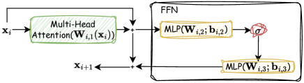
Figure 2: The process of Transformer

In this section, we will detail how to convert 2D convolution operations into their corresponding matrix-vector forms, focusing on two scenarios: 1-O and I-O. To clearly describe the 2D convolution process, we first outline the general procedure and some basic conventions. The general process of 2D convolution involves convolving a kernel with the input data and then summing along the input channel direction (referred to as the $C_{I}$ direction) to obtain an element in the output. The convolution kernel slides along the height ($H$) and width ($W$) directions to produce the entire output feature map. To generate multiple feature maps, multiple sets of convolution kernels, $C_{O}$, are required, with each set having the same number of channels as the input channels. Depending on the context, $C_{I}$, $C_{O}$, $H$, and $W$ can represent either the corresponding dimension directions or the number of dimensions in those directions. Figures 2 and 3 illustrate the conversion process for each case, transforming them into matrix-vector representations.

Specifically, Figure 2.a shows the process of 1-O Conv2D. Here, $\mathbf{W}_{1}\cdots\mathbf{W}_{O}$ represent the convolution kernels, which slide across the input data along the $H$ and $W$ directions. For a single-channel input producing $O$ output channels, $O$ convolution kernels are each convolved with the same input $\mathbf{x}$ to produce outputs $\mathbf{y}_{1}\cdots\mathbf{y}_{O}$. Figure 2.b provides an example of a 1-O Conv2D. Additionally, Figure 2.c further converts the example given in Figure 2.b into its corresponding matrix-vector form. Therefore, it is straightforward to derive the matrix-vector form of 1-O Conv2D as follows:

$$\left(\begin{array}[]{cccc}\mathbf{W}_{1}^{\prime}&\mathbf{W}_{2}^{\prime}&\cdots\mathbf{W}_{O}^{\prime}\end{array}\right)\diamond\mathbf{x}^{\prime}=\left(\begin{array}[]{cccc}\mathbf{y}_{1}^{\prime}\\ \mathbf{y}_{2}^{\prime}\\ \vdots\\ \mathbf{y}_{O}^{\prime}\end{array}\right)$$ (1)

Figure 3.a depicts the general process of I-O Conv2D, considering the scenario with $I$ input channels and $O$ output channels. This requires $O$ sets of convolution kernels, each set containing $I$ kernels, collectively represented as $\mathbf{W}_{1,1}\cdots\mathbf{W}_{1,I}\cdots\mathbf{W}_{O,1}\cdots\mathbf{W}_{O,I}$. Each kernel $\mathbf{W}_{i,j}$ with indices $i,j$ convolves with the $j$-th input channel $\mathbf{x}_{j}$ to produce an intermediate output $\mathbf{y}_{i,j}$. Summing all intermediate outputs $\mathbf{y}_{i,1}\cdots\mathbf{y}_{i,I}$ in the $i$-th set yields the final $i$-th output channel $\mathbf{y}_{i}$. Figure 3.b provides a simplified example. Subsequently, Figure 3.c presents the corresponding matrix-vector representation for the example in Figure 3.b. Therefore, the matrix-vector formula for I-O Conv2D can be expressed as follows:

$$\left(\begin{array}[]{cccccc}\mathbf{W}_{1,1}^{\prime}&\mathbf{W}_{2,1}^{\prime}&\cdots&\mathbf{W}_{O,1}^{\prime}\\ \mathbf{W}_{1,2}^{\prime}&\mathbf{W}_{2,2}^{\prime}&\cdots&\mathbf{W}_{O,2}^{\prime}\\ \vdots&\vdots&\vdots&\vdots\\ \mathbf{W}_{1,I}^{\prime}&\mathbf{W}_{2,I}^{\prime}&\cdots&\mathbf{W}_{O,I}^{\prime}\end{array}\right)\diamond\left(\begin{array}[]{c}\mathbf{x}_{1}^{\prime}\\ \mathbf{x}_{2}^{\prime}\\ \vdots\\ \mathbf{x}_{I}^{\prime}\end{array}\right)=\left(\begin{array}[]{c}\mathbf{y}_{1}^{\prime}\\ \mathbf{y}_{2}^{\prime}\\ \vdots\\ \mathbf{y}_{O}^{\prime}\end{array}\right)$$ (2)

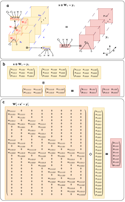
Figure 4: 1-O Conv3D process and the matrix-vector transformation example.

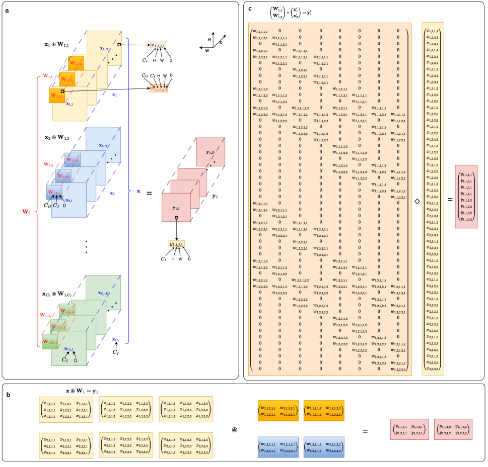
Figure 5: I-1 Conv3D process and the matrix-vector transformation example.

3.2 The Matrix-Vector Method for Conv3D

3D convolution is a structure designed primarily for video or 3D image data, consisting mainly of two forms: 1-O Conv3D and I-O Conv3D. Given their complexity, we provide proof examples only for the 1-1 and I-1 Conv3D forms. The forms of 1-O and I-O Conv3D can be easily derived from the 1-1 and I-1 Conv3D forms. Compared with 2D convolution, 3D convolution has an additional depth dimension ($D$). So the convolution kernel could slide along with $H,W,D$, and it also needs to sum in $C_{I}$ direction.

Figure 4 illustrates the process of converting 1-1 Conv3D into its matrix-vector form. Figure 4.a shows the general form of 1-O Conv3D. As a 3D convolution, the input data typically has four dimensions: $(C_{I},H,W,D)$, representing the number of input channels, height, width, and depth, respectively. In 1-1 Conv3D, $C_{I}$ is at most 1. The convolution kernel has an additional dimension $C_{O}$, representing the number of output channels, and in this case, $C_{O}=1$. The convolution kernel slides along the width (W), height (H), and depth (D) directions. Figure 4.b presents a specific example, while Figure 4.c converts this example into its matrix-vector form (ignoring changes in H, W, D dimensions due to lack of padding).

According to Figure 4, the matrix-vector form of 1-O Conv3D can be easily derived and is consistent with Eq. (1). The difference lies in the fact that $\mathbf{W}_{i}$ has depth, so the corresponding $\mathbf{W}_{i}^{\prime}$ needs to be recombined as shown in Figure 4.c.

Similarly, Figures 5.a, b, and c illustrate the general process, a simple example, and the corresponding matrix-vector form of I-1 Conv3D, respectively. According to Figure 5, the matrix-vector form of I-O Conv3D is consistent with (1). The difference is that both $\mathbf{x}_{i}$ and $\mathbf{W}_{i}$ have depth, so the corresponding $\mathbf{x}_{i}^{\prime}$ and $\mathbf{W}_{i}^{\prime}$ need to be obtained as shown in Figure 5.c.

3.3 The Matrix-Vector Method for Mean Pooling

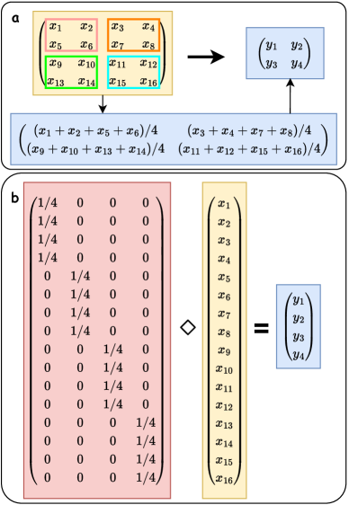
Figure 6: Mean pooling process and the matrix-vector transformation example.

Mean pooling is also an important technique in the field of CV, often used in conjunction with convolution. To demonstrate that CNNs can be expressed in the form of UAT, we need to prove that mean pooling can also be represented in matrix-vector form. In Figure 6, we provide an example. Figure 6.a shows the process of mean pooling, while Figure 6.b illustrates its corresponding matrix-vector form. Based on Figure 6, we can conclude that mean pooling can indeed be represented in matrix-vector form.

3.4 Transformer for CV

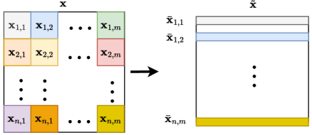
Figure 7: The MHA operation in CV.

In UAT2LLMs, it has been demonstrated that the feedforward network (FFN) and MHA components in the Transformer architecture can be represented in matrix-vector form. Given that ViTs are also based on the Transformer framework, we only need to focus on the differences between Transformers in CV and those in UAT2LLMs. A key feature of ViTs is that they divide the original image into multiple patches: $\mathbf{x}_{1,1},\cdots,\mathbf{x}_{n,m}$. Each image patch is then reshaped into row vectors $\bar{\mathbf{x}}_{1,1},\cdots,\bar{\mathbf{x}}_{n,m}$, which are concatenated along the column direction to obtain $\tilde{\mathbf{x}}$, as shown in Figure 7. MHA and FFN operations are then applied, so aside from the initial processing part, the subsequent transformation process completely follows the description in UAT2LLMs. Therefore, it is easy to deduce that ViTs are also specific implementations of the UAT.

3.5 Summary

We have demonstrated that various modules in CV, including 2D convolution, 3D convolution, mean pooling, MHA, and FFN, can all be represented by diamond matrix multiplication. Considering the relationship between diamond matrix multiplication and matrix multiplication: $\mathbf{W}\diamond\mathbf{x}=\mathbf{W}^{T}\mathbf{x}$. Therefore, unless otherwise specified, we will conveniently use $\mathbf{W}^{\prime}\mathbf{x}^{\prime}$ to represent the matrix-vector form of them. Here, $\mathbf{W}^{\prime}$ is derived from the parameters $\mathbf{W}$ of the various modules, and $\mathbf{x}^{\prime}$ is derived from the inputs $\mathbf{x}$ of the modules.

4 Discussion

In this section, we will answer the questions in the field of CV proposed in the Introduction.

4.1 Why must CNNs be Deep?

There are two main reasons why CNNs typically have deep layers. The first reason stems from the learning paradigm of CNNs. The design of CNNs is based on two well-known principles: local receptive fields (i.e., local features in images often contain important information) and spatial invariance (these important local features can appear anywhere in the image). These principles necessitate learning from each small region of the image, with all small regions sharing the same parameters. If parameters differed, it would imply that a certain object must appear in a specific part of the image, which is clearly unreasonable.

The above reasons dictate that image learning occurs in small patches, which explains why convolutional kernels are typically small. However, if the network has only a few layers, such as a single layer, it means that each small patch is learned independently. We know that objects in an image are generally composed of multiple such patches. Observing only a part of the image cannot provide a clear identification of the object. Therefore, a larger receptive field is needed, which can be achieved by increasing the number of layers to gather global information.

The second reason is derived from the UAT. As shown in Figure 1, increasing the number of layers in the network means a larger $N$, which brings the UAT closer to approximating the target function. An image can be understood as a special function in a high-dimensional space, exhibiting strong correlations in 2D or 3D space. These two reasons are also applicable to ViTs. Figure 7 shows the preprocessing of ViTs, where $\tilde{\mathbf{x}}$ is the input to the ViTs. It is evident that each row shares the same parameters, and the learning of each row adheres to the principles of local receptive fields and spatial invariance.

4.2 Why Residual-Based CNNs Excel in CV: Superior Generalization Ability

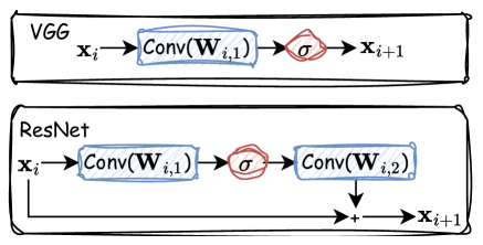
Figure 8: VGG Vs ResNet: The characters in ’()’ represent the corresponding operation’s parameters. Hereinafter the same.

In the previous discussion, we explained why deep networks are essential for learning in CNNs. However, why did VGG, despite being a deep network, not dominate the subsequent development of CV, whereas residual-based CNNs did? ResNet, one of the most influential architectures in the field, has significantly shaped the design of later network architectures, with the residual structure appearing in many subsequent networks. What exactly endows the residual structure with such powerful capabilities? We think the answer is the generalization capability given by residual structure. To analyze the source of this power, we use the Matrix-Vector Method to express parts of VGG and the residual structure in corresponding equations, and then compare them with the UAT.

Figure 8 illustrates the basic structures of VGG and ResNet. Based on this figure, a three-layer VGG can be written as Eq.(3), which perfectly aligns with the multilayer UAT mathematical form proposed by Hornik (Hornik, Stinchcombe, and White 1989). On the other hand, a two-layer Residual-based CNNs can be expressed in the form shown in Eq.(4) (see Appendix A.1 for detail.), conforming to the UAT form given in Figure 1. In this equation, $\hat{\mathbf{b}}_{i+1,1}$ is calculated from $\mathbf{W}_{i,1}^{\prime},\mathbf{W}_{i,2}^{\prime},\mathbf{x}^{\prime}_{i},\mathbf{b}_{i,1},\mathbf{b}_{i,2},\mathbf{b}_{i+1,1}$. It is evident that both VGG and ResNet are concrete implementations of UAT. Theoretically, their approximation capabilities should be equivalent, and any differences could be mitigated by increasing the number of network layers. So why is ResNet significantly more powerful than VGG?

$$\mathbf{x}^{\prime}_{i+3} =\sigma(\mathbf{W}^{\prime}_{i+2}[\sigma(\mathbf{W}^{\prime}_{i+1}\sigma(\mathbf{W}^{\prime}_{i}\mathbf{x}^{\prime}_{i}+\mathbf{b}^{\prime}_{i})+\mathbf{b}^{\prime}_{i+1})]$$ (3)

$$+\mathbf{b}^{\prime}_{i+2})$$

$$\mathbf{x}^{\prime}_{i+2} =\mathbf{x}_{i}^{\prime}+\mathbf{W}_{i,2}^{\prime}\sigma(\mathbf{W}_{i,1}^{\prime}\mathbf{x}^{\prime}_{i}+\mathbf{b}_{i,1})+\mathbf{W}_{i,2}^{\prime}\sigma(\mathbf{W}_{i,1}^{\prime}\mathbf{x}_{i}^{\prime}$$ (4)

$$+\hat{\mathbf{b}}_{i+1,1})+\overline{\mathbf{b}}_{i+1,2}$$

The primary reason lies in the dynamic approximation capabilities of residual networks. As seen in Eq. (3), once a VGG network is trained, its corresponding UAT parameters are fixed. This means that a VGG network can only approximate a single, fixed function. Although UAT has strong approximation abilities, image data is highly variable, and the corresponding function often changes. In contrast, residual networks can dynamically approximate the corresponding function based on the input because the biases in residual networks are influenced by the input. For example, in Eq. (4), $\hat{\mathbf{b}}_{i+1,1}$ is affected by the input $\mathbf{x}^{\prime}_{i}$.

For convenience, we do not explicitly show which parameters influence other parameters in the final merged mathematical expression of the model. If a parameter in the UAT model is influenced only by other network parameters, it can be considered fixed once the network is trained. We denote such parameters with an overline, such as $\overline{\mathbf{W}}$. If a parameter in the UAT model is influenced by the input, we denote it with a hat, such as $\hat{\mathbf{b}}$.

Therefore, while the original UAT formula has strong approximation capabilities, using it for approximation (equivalent to using a VGG network in CV) means that once training is complete, the UAT parameters are fixed, and the function it can approximate is also fixed. In contrast, in residual networks, the UAT parameters can change based on the input, allowing the function being approximated to vary accordingly. This adaptability is the fundamental source of the superiority of residual networks.

4.3 The Difference between Residual-Based CNNs and ViTs

Figure 9: The process of Transformer.

In the previous section, we used the matrix-vector method to represent VGG and ResNet in their corresponding mathematical forms and analyzed them from the perspective of the UAT. In this section, we will apply the same method to analyze the Transformer in ViTs and compare it with residual-based CNNs. Figure 9 shows the general form of a Transformer. After derivation, the mathematical form of a two-layer Transformer network corresponds to Eq. (5) (see Appendix A.2 for detail.). Clearly, the mathematical representation of ViT also conforms to UAT, with some parameters influenced by the input information.

The main difference between Transformer networks and residual-based multi-layer convolutional networks lies in how input information affects their corresponding UAT parameters. In Transformer networks, input information influences both weight and bias in the corresponding UAT. In contrast, in networks constructed with multiple residual convolutions, input information only influences bias in the corresponding UAT. Essentially, both types of networks have the ability to dynamically approximate functions based on input. This aligns with their nearly identical performance in the field of CV, supporting the theoretical foundation that both are specific implementations of UAT capable of dynamically approximating the corresponding functions based on input.

$$\mathbf{x}^{\prime}_{i+2} =\hat{\mathbf{W}}^{\prime}_{i+1,1}\mathbf{x}^{\prime}_{i}+\hat{\mathbf{W}}^{\prime}_{i+1,2}\sigma(\hat{\mathbf{W}}^{\prime}_{i,1}\mathbf{x}^{\prime}_{i}+\mathbf{b}^{\prime}_{i,2})+\hat{\mathbf{b}}^{\prime}_{i,1}$$ (5)

$$+\mathbf{W}^{\prime}_{i+1,3}\sigma(\hat{\mathbf{W}}^{\prime}_{i+1,3}\mathbf{x}^{\prime}_{i}+\hat{\mathbf{b}}^{\prime}_{i+1,2})$$

4.4 The Theory behind Lora and Pruning

In UAT2LLMs, UAT has been used to explain why LoRA and pruning are feasible. In the field of CV, we have proven that both convolution-based CNNs and Transformer-based ViTs are concrete implementations of UAT. Therefore, the principles behind LoRA and pruning in CV are the same as those mentioned in UAT2LLMs. Specifically, LoRA works by layer-wise adjustment of parameters, while pruning is effective because some layer parameters have minimal impact on the overall result.

5 Conclusion

This paper delves into the theoretical foundations of deep learning in the field of CV. Specifically, the current CV landscape is primarily dominated by CNNs and Transformer models. We utilize the matrix-vector method to unify these models under the framework of the UAT. Based on this framework, we provide explanations for several common issues and techniques in CV. The requirement for deep networks in CNNs is jointly determined by the intrinsic characteristics of image data and the demands of UAT theory. The robust generalization ability of residual networks stems from their ingenious design, which enables UAT to dynamically adapt to corresponding functions based on input data. Similarly, Transformer-based models possess this ability, with the key difference lying in which parameters of UAT they influence. Residual networks primarily affect the bias term, while Transformers influence both the weights and the bias. Additionally, the feasibility of LoRA operations in CV arises because it can fine-tune the parameters of different UAT layers based on input data characteristics. The viability of pruning techniques is due to the fact that the parameters of certain network layers have minimal impact on the final outcome.

Appendix A The UAT Format of Residual-based CNNs and Transformer-based ViTs

In this section, we will present the Matrix-Vector form of residual-based CNNs and Transformer-based ViTs and their relationship with the UAT. Figure 1 and 2 show a schematic of a residual-based convolution and Transformer. We have already established that convolution and components in a Transformer can be represented in a matrix-vector form. Therefore, to illustrate its relationship with UAT, we will use Figure 1 and 2, with the input $\mathbf{x}_{i}$, derive the mathematical form corresponding to $\mathbf{x}_{i+2}$. We will express this in matrix-vector form, so parameters and inputs/outputs will have a prime (^′) in the upper right corner to indicate their matrix-vector form.

Due to the complexity of the variables involved, we will combine some terms to align the resulting equations with the standard UAT form. To distinguish these parameter variables, we will keep the original variables unchanged. If a parameter variable is influenced only by other variables, we will denote it with a bar on top, such as $\bar{\mathbf{W}}$. If it is influenced by the input $\mathbf{x}_{i}$, we will mark it with a hat, such as $\hat{\mathbf{W}}$.

A.1 The UAT Format of Residual-based CNNs

Through derivation and simplification, we obtain the matrix-vector mathematical representation for $\mathbf{x}_{i+2}$, as shown in Eq.1. Comparing this with the standard UAT form, it is evident that the parameters in UAT are fixed after training. In contrast, the bias terms in the UAT corresponding to residual-based CNNs can change dynamically based on the input.

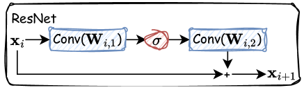
Figure 1: The process of residual-base convolutional block.

$$\mathbf{x}^{\prime}_{i+1} =\mathbf{x}_{i}^{\prime}+\mathbf{W}_{i,2}^{\prime}\sigma(\mathbf{W}_{i,1}^{\prime}\mathbf{x}^{\prime}_{i}+\mathbf{b}_{i,1})+\mathbf{b}_{i,2}$$ (1)

$$\mathbf{x}^{\prime}_{i+2} =\mathbf{x}^{\prime}_{i+1}+\mathbf{W}_{i,2}^{\prime}\sigma(\mathbf{W}_{i,1}^{\prime}\mathbf{x}^{\prime}_{i+1}+\mathbf{b}_{i+1,1})+\mathbf{b}_{i+1,2}$$

$$=[\mathbf{x}_{i}^{\prime}+\mathbf{W}_{i,2}^{\prime}\sigma(\mathbf{W}_{i,1}^{\prime}\mathbf{x}^{\prime}_{i}+\mathbf{b}_{i,1})+\mathbf{b}_{i,2}]$$

$$+\mathbf{W}_{i,2}^{\prime}\sigma(\mathbf{W}_{i,1}^{\prime}[\mathbf{x}_{i}^{\prime}+\mathbf{W}_{i,2}^{\prime}\sigma(\mathbf{W}_{i,1}^{\prime}\mathbf{x}^{\prime}_{i}+\mathbf{b}_{i,1})+\mathbf{b}_{i,2}]+\mathbf{b}_{i+1,1})+\mathbf{b}_{i+1,2}$$

$$=\mathbf{x}_{i}^{\prime}+\mathbf{W}_{i,2}^{\prime}\sigma(\mathbf{W}_{i,1}^{\prime}\mathbf{x}^{\prime}_{i}+\mathbf{b}_{i,1})+\mathbf{b}_{i,2}$$

$$+\mathbf{W}_{i,2}^{\prime}\sigma(\mathbf{W}_{i,1}^{\prime}\mathbf{x}_{i}^{\prime}+\mathbf{W}_{i,1}^{\prime}\mathbf{W}_{i,2}^{\prime}\sigma(\mathbf{W}_{i,1}^{\prime}\mathbf{x}^{\prime}_{i}+\mathbf{b}_{i,1})+\mathbf{W}_{i,1}^{\prime}\mathbf{b}_{i,2}+\mathbf{b}_{i+1,1})+\mathbf{b}_{i+1,2}$$

$$=\mathbf{x}_{i}^{\prime}+\mathbf{W}_{i,2}^{\prime}\sigma(\mathbf{W}_{i,1}^{\prime}\mathbf{x}^{\prime}_{i}+\mathbf{b}_{i,1})+\mathbf{W}_{i,2}^{\prime}\sigma(\mathbf{W}_{i,1}^{\prime}\mathbf{x}_{i}^{\prime}+\hat{\mathbf{b}}_{i+1,2})+\overline{\mathbf{b}}_{i+1,2}$$

A.2 The UAT Format of Transformer-based ViTs

Eq.(2) and (3) give an example of the matrix-vector format of MHA and FFN. Eq. (4) give the corresponding matrix-vector format of $\mathbf{x}_{i+2}$. It is obvious that the bias and weight terms in the UAT corresponding to Transformed-based ViTs can change dynamically based on the input.

$$MHA(\mathbf{x}^{\prime}_{i})=\mathbf{W}^{\prime}_{i,1}\mathbf{x}^{\prime}_{i}\\$$ (2)

$$FFN(\mathbf{x}^{\prime}_{i})=\mathbf{W}^{\prime}_{i,3}\sigma(\mathbf{W}^{\prime}_{i,2}\mathbf{x}^{\prime}_{i}+\mathbf{b}^{\prime}_{i,2})+\mathbf{b}^{\prime}_{i,3}\\$$ (3)

$$\mathbf{x}^{\prime}_{i+1} =\mathbf{W}^{\prime}_{i,1}\mathbf{x}^{\prime}_{i}+\mathbf{W}^{\prime}_{i,3}\sigma(\mathbf{W}^{\prime}_{i,2}[\mathbf{W}^{\prime}_{i,1}\mathbf{x}^{\prime}_{i}]+\mathbf{b}^{\prime}_{i,2})+\mathbf{b}^{\prime}_{i,3}$$ (4)

$$=\mathbf{W}^{\prime}_{i,1}\mathbf{x}^{\prime}_{i}+\mathbf{W}^{\prime}_{i,3}\sigma(\hat{\mathbf{W}}^{\prime}_{i,1}\mathbf{x}^{\prime}_{i}+\mathbf{b}^{\prime}_{i,2})+\mathbf{b}^{\prime}_{i,3}$$

$$\mathbf{x}^{\prime}_{i+2} =\mathbf{W}^{\prime}_{i+1,1}\mathbf{x}^{\prime}_{i+1}+\mathbf{W}^{\prime}_{i+1,3}\sigma(\mathbf{W}^{\prime}_{i+1,2}[\mathbf{W}^{\prime}_{i+1,1}\mathbf{x}^{\prime}_{i+1}]+\mathbf{b}^{\prime}_{i+1,2})+\mathbf{b}^{\prime}_{i+1,3}$$

$$=\mathbf{W}^{\prime}_{i+1,1}\mathbf{x}^{\prime}_{i+1}+\mathbf{W}^{\prime}_{i+1,3}\sigma(\hat{\mathbf{W}}^{\prime}_{i+1,1}\mathbf{x}^{\prime}_{i+1}+\mathbf{b}^{\prime}_{i+1,2})+\mathbf{b}^{\prime}_{i+1,3}$$

$$=\mathbf{W}^{\prime}_{i+1,1}[\mathbf{W}^{\prime}_{i,1}\mathbf{x}^{\prime}_{i}+\mathbf{W}^{\prime}_{i,3}\sigma(\hat{\mathbf{W}}^{\prime}_{i,1}\mathbf{x}^{\prime}_{i}+\mathbf{b}^{\prime}_{i,2})+\mathbf{b}^{\prime}_{i,3}]$$

$$+\mathbf{W}^{\prime}_{i+1,3}\sigma(\hat{\mathbf{W}}^{\prime}_{i+1,1}[\mathbf{W}^{\prime}_{i,1}\mathbf{x}^{\prime}_{i}+\mathbf{W}^{\prime}_{i,3}\sigma(\hat{\mathbf{W}}^{\prime}_{i,1}\mathbf{x}^{\prime}_{i}+\mathbf{b}^{\prime}_{i,2})+\mathbf{b}^{\prime}_{i,3}]+\mathbf{b}^{\prime}_{i+1,2})+\mathbf{b}^{\prime}_{i+1,3}$$

$$=\hat{\mathbf{W}}^{\prime}_{i+1,1}\mathbf{x}^{\prime}_{i}+\hat{\mathbf{W}}^{\prime}_{i+1,2}\sigma(\hat{\mathbf{W}}^{\prime}_{i,1}\mathbf{x}^{\prime}_{i}+\mathbf{b}^{\prime}_{i,2})+\hat{\mathbf{b}}^{\prime}_{i,1}$$

$$+\mathbf{W}^{\prime}_{i+1,3}\sigma(\hat{\mathbf{W}}^{\prime}_{i+1,3}\mathbf{x}^{\prime}_{i}+\hat{\mathbf{b}}^{\prime}_{i+1,2})$$

References

- Bai et al. (2022) Bai, J.; Yuan, L.; Xia, S.-T.; Yan, S.; Li, Z.; and Liu, W. 2022. Improving vision transformers by revisiting high-frequency components. In European Conference on Computer Vision, 1–18. Springer.
- Cybenko (2007) Cybenko, G. 2007. Approximation by superpositions of a sigmoidal function. Mathematics of Control, Signals, and Systems, 303–314.
- Dosovitskiy et al. (2020) Dosovitskiy, A.; Beyer, L.; Kolesnikov, A.; Weissenborn, D.; Zhai, X.; Unterthiner, T.; Dehghani, M.; Minderer, M.; Heigold, G.; Gelly, S.; et al. 2020. An image is worth 16x16 words: Transformers for image recognition at scale. arXiv preprint arXiv:2010.11929.
- Gao et al. (2019) Gao, S.; Cheng, M.-M.; Zhao, K.; Zhang, X.; Yang, M.-H.; and Torr, P. H. S. 2019. Res2Net: A New Multi-Scale Backbone Architecture. IEEE Transactions on Pattern Analysis and Machine Intelligence, 43: 652–662.
- He et al. (2016) He, K.; Zhang, X.; Ren, S.; and Sun, J. 2016. Deep residual learning for image recognition. In Proceedings of the IEEE conference on computer vision and pattern recognition, 770–778.
- Hornik, Stinchcombe, and White (1989) Hornik, K.; Stinchcombe, M. B.; and White, H. L. 1989. Multilayer feedforward networks are universal approximators. Neural Networks, 2: 359–366.
- Hou et al. (2024) Hou, X.; Liu, M.; Zhang, S.; Wei, P.; and Chen, B. 2024. Salience DETR: Enhancing Detection Transformer with Hierarchical Salience Filtering Refinement. ArXiv, abs/2403.16131.
- Huang et al. (2023) Huang, T.; Yin, L.; Zhang, Z. A.; Shen, L.; Fang, M.; Pechenizkiy, M.; Wang, Z.; and Liu, S. 2023. Are Large Kernels Better Teachers than Transformers for ConvNets? In International Conference on Machine Learning.
- Kim et al. (2024) Kim, M.; Seo, P. H.; Schmid, C.; and Cho, M. 2024. Learning Correlation Structures for Vision Transformers. ArXiv, abs/2404.03924.
- Krizhevsky, Sutskever, and Hinton (2017) Krizhevsky, A.; Sutskever, I.; and Hinton, G. E. 2017. ImageNet classification with deep convolutional neural networks. Commun. ACM, 60(6): 84–90.
- Lecun et al. (1998) Lecun, Y.; Bottou, L.; Bengio, Y.; and Haffner, P. 1998. Gradient-based learning applied to document recognition. Proceedings of the IEEE, 86(11): 2278–2324.
- Liu et al. (2021) Liu, Z.; Lin, Y.; Cao, Y.; Hu, H.; Wei, Y.; Zhang, Z.; Lin, S.; and Guo, B. 2021. Swin Transformer: Hierarchical Vision Transformer using Shifted Windows. 2021 IEEE/CVF International Conference on Computer Vision (ICCV), 9992–10002.
- Lv et al. (2023) Lv, W.; Xu, S.; Zhao, Y.; Wang, G.; Wei, J.; Cui, C.; Du, Y.; Dang, Q.; and Liu, Y. 2023. DETRs Beat YOLOs on Real-time Object Detection. ArXiv, abs/2304.08069.
- Minaee et al. (2021) Minaee, S.; Boykov, Y.; Porikli, F.; Plaza, A.; Kehtarnavaz, N.; and Terzopoulos, D. 2021. Image segmentation using deep learning: A survey. IEEE transactions on pattern analysis and machine intelligence, 44(7): 3523–3542.
- Nah et al. (2019) Nah, S.; Baik, S.; Hong, S.; Moon, G.; Son, S.; Timofte, R.; and Mu Lee, K. 2019. Ntire 2019 challenge on video deblurring and super-resolution: Dataset and study. In Proceedings of the IEEE/CVF conference on computer vision and pattern recognition workshops, 0–0.
- Park and Kim (2022) Park, N.; and Kim, S. 2022. How do vision transformers work? arXiv preprint arXiv:2202.06709.
- Rawat and Wang (2017) Rawat, W.; and Wang, Z. 2017. Deep convolutional neural networks for image classification: A comprehensive review. Neural computation, 29(9): 2352–2449.
- Ren et al. (2015) Ren, S.; He, K.; Girshick, R. B.; and Sun, J. 2015. Faster R-CNN: Towards Real-Time Object Detection with Region Proposal Networks. IEEE Transactions on Pattern Analysis and Machine Intelligence, 39: 1137–1149.
- Russakovsky et al. (2014) Russakovsky, O.; Deng, J.; Su, H.; Krause, J.; Satheesh, S.; Ma, S.; Huang, Z.; Karpathy, A.; Khosla, A.; Bernstein, M. S.; Berg, A. C.; and Fei-Fei, L. 2014. ImageNet Large Scale Visual Recognition Challenge. International Journal of Computer Vision, 115: 211 – 252.
- Shi (2023) Shi, D. 2023. TransNeXt: Robust Foveal Visual Perception for Vision Transformers. ArXiv, abs/2311.17132.
- Simonyan and Zisserman (2014) Simonyan, K.; and Zisserman, A. 2014. Very Deep Convolutional Networks for Large-Scale Image Recognition. CoRR, abs/1409.1556.
- Szegedy et al. (2014) Szegedy, C.; Liu, W.; Jia, Y.; Sermanet, P.; Reed, S. E.; Anguelov, D.; Erhan, D.; Vanhoucke, V.; and Rabinovich, A. 2014. Going deeper with convolutions. 2015 IEEE Conference on Computer Vision and Pattern Recognition (CVPR), 1–9.
- Vaswani et al. (2017) Vaswani, A.; Shazeer, N. M.; Parmar, N.; Uszkoreit, J.; Jones, L.; Gomez, A. N.; Kaiser, L.; and Polosukhin, I. 2017. Attention is All you Need. In Neural Information Processing Systems.
- Wang et al. (2023) Wang, A.; Chen, H.; Lin, Z.; Pu, H.; and Ding, G. 2023. RepViT: Revisiting Mobile CNN From ViT Perspective. ArXiv, abs/2307.09283.
- Wang et al. (2017) Wang, F.; Jiang, M.; Qian, C.; Yang, S.; Li, C.; Zhang, H.; Wang, X.; and Tang, X. 2017. Residual attention network for image classification. In Proceedings of the IEEE conference on computer vision and pattern recognition, 3156–3164.
- Wang et al. (2022a) Wang, R.; Lei, T.; Cui, R.; Zhang, B.; Meng, H.; and Nandi, A. K. 2022a. Medical image segmentation using deep learning: A survey. IET Image Processing, 16(5): 1243–1267.
- Wang et al. (2019a) Wang, T.-C.; Liu, M.-Y.; Tao, A.; Liu, G.; Kautz, J.; and Catanzaro, B. 2019a. Few-shot video-to-video synthesis. arXiv preprint arXiv:1910.12713.
- Wang et al. (2018) Wang, T.-C.; Liu, M.-Y.; Zhu, J.-Y.; Liu, G.; Tao, A.; Kautz, J.; and Catanzaro, B. 2018. Video-to-video synthesis. arXiv preprint arXiv:1808.06601.
- Wang and Li (2024) Wang, W.; and Li, Q. 2024. Universal Approximation Theory: The basic theory for large language models. arXiv:2407.00958.
- Wang et al. (2019b) Wang, X.; Chan, K. C.; Yu, K.; Dong, C.; and Change Loy, C. 2019b. Edvr: Video restoration with enhanced deformable convolutional networks. In Proceedings of the IEEE/CVF conference on computer vision and pattern recognition workshops, 0–0.
- Wang et al. (2022b) Wang, Z.; Bai, Y.; Zhou, Y.; and Xie, C. 2022b. Can CNNs Be More Robust Than Transformers? ArXiv, abs/2206.03452.
- Wei et al. (2016) Wei, X.-S.; Luo, J.-H.; Wu, J.; and Zhou, Z.-H. 2016. Selective Convolutional Descriptor Aggregation for Fine-Grained Image Retrieval. IEEE Transactions on Image Processing, 26: 2868–2881.
- Xie et al. (2016) Xie, S.; Girshick, R. B.; Dollár, P.; Tu, Z.; and He, K. 2016. Aggregated Residual Transformations for Deep Neural Networks. 2017 IEEE Conference on Computer Vision and Pattern Recognition (CVPR), 5987–5995.
- Xu, Zhang, and Xiao (2019) Xu, Z.-Q. J.; Zhang, Y.; and Xiao, Y. 2019. Training behavior of deep neural network in frequency domain. In Neural Information Processing: 26th International Conference, ICONIP 2019, Sydney, NSW, Australia, December 12–15, 2019, Proceedings, Part I 26, 264–274. Springer.
- Yin et al. (2019) Yin, D.; Gontijo Lopes, R.; Shlens, J.; Cubuk, E. D.; and Gilmer, J. 2019. A fourier perspective on model robustness in computer vision. Advances in Neural Information Processing Systems, 32.