Analytical reconstruction of equivalent purely kinetic k-essence description for $c_{s}^{2}(w)$ barotropic fluid models

Abstract

A novel approach to the class of cosmic barotropic fluids in which the speed of sound squared is defined as a function of the Equation of State parameter, so called $c_{s}^{2}(w)$ models, is examined. For this class of models, a new analytical reconstruction method is introduced for finding their equivalent purely kinetic k-essence formulation. The method is explicitly demonstrated for several $c_{s}^{2}(w)$ models. The application of the obtained explicit or closed form solutions in understanding dark sector unification models is discussed.

1 Introduction

One of most dramatic shifts in physical understanding of the universe happened with the discovery of its late-time accelerated expansion. Despite the mounting observational evidence of the speed-up in the global cosmic dynamics [1, 2, 3, 4, 5], the question of precise mechanism causing the cosmic acceleration remains unanswered. Among numerous proposals for the said mechanism, two most prominent approaches are the presence of a cosmic component with a negative pressure, called dark energy [6, 7, 8, 9, 10] and the modifications of gravitational interaction at cosmic distances [11, 12, 13].

An older, though not less enigmatic, challenge is evident in increased gravitational interaction without a visible source at various scales in galactic and galaxy cluster dynamics, as well as in the cosmic history of growth of inhomogeneities and large scale structure formation. The most studied approach is the presence of a cosmic component, called dark matter [14, 15, 16, 17], although alternatives exist, with MOND and its generalizations being the most notable one [18, 19, 20, 21, 22].

A cosmic model assuming that dark energy is a small positive cosmological constant and that dark matter comes in the form of cold dark matter, known as the $\Lambda$CDM model, has occupied a central place in cosmology for more than two decades owing to its simplicity and explanatory power. However, ever more precise and more abundant cosmic observations have revealed inadequacies of this model, e.g. in the form of so called $H_{0}$ tension [23, 24, 25, 26]. Recent years have brought a large number of various attempts beyond the $\Lambda$CDM model, questioning and extending all its assumptions.

An idea of a single cosmic component unifying the concepts of dark matter and dark energy is attractive, both for fundamental and practical reasons, see e.g. [27]. A further assumption that this cosmic component unifying the dark sector can be described as a barotropic perfect fluid [28] comes naturally since other cosmic components such as non-relativistic matter or radiation allow such a description. One of such early and prominent examples of barotropic fluid unifications is the Chaplygin gas [29, 30] and its numerous generalizations [31, 32, 33, 34, 35] (see also [36] for early strong obsevational bounds).

Recent works [37] also claim that the concept of dark energy is underdetermined, i.e. that available cosmological observations cannot fully constrain microscopic dark energy models. The best description of dark energy, then, is of phenomenological character. In view of such claims (but also as a generally sound phenomenological approach), it is important to approach dark sector model building in a way that is consistent with observational data. Very rough and somewhat simplified categorization of observational signals in cosmology could be to those that inform us on the cosmic global expansion and those that provide insight into structure formation and growth. For a dark sector unified component being a barotropic perfect fluid, the global expansion of the universe is influenced by its Equation of State parameter $w\equiv p/\rho$, whereas the quantity of importance with respect to structure growth is its adiabatic speed of sound $c_{s}^{2}\equiv\frac{dp}{d\rho}$. Therefore, it seems phenomenologically advantageous to develop models where these two quantities are related, i.e. where $c_{s}^{2}$ is a function of $w$. The usefulness of these models, called $c_{s}^{2}(w)$ models, has already been demonstrated in the study of dark sector unifications [38, 39, 40], cosmological constant barrier crossing [41], physical viability of dark energy parametrizations [42] and analysis of galaxy rotation curves in models where dark matter is a barotropic fluid [43].

A powerful field-theoretical framework for description of the dark sector and its dynamics, based on the generalized kinetic term of the scalar filed, is known as k-essence. K-essence was successfully applied in description of inflation [44, 45], dark energy [46, 47, 48, 49, 50, 51, 52], unified dark sector [53, 54, 55, 56, 57, 58, 59] and tachyons [60, 61, 62, 63] An equivalent microscopic description of $c_{s}^{2}(w)$ models can be obtained in the framework of purely kinetic k-essence [64, 65, 66]. A detailed presentation of a general approach how to translate $c_{s}^{2}(w)$ to purely kinetic k-essence models was given in [40], together with a concrete analytic demonstration of the approach for a number of $c_{s}^{2}(w)$ models. In this paper we introduce a novel method for the reconstruction of purely kinetic k-essence for the known $c_{s}^{2}(w)$ models. The presentation of the general method is followed by its application to five $c_{s}^{2}(w)$ models.

The structure of this paper is the following. The first section is the introduction. The method of reconstructing of equivalent purely kinetic k-essence is presented in the second section. The third section brings the application of the method developed in the second section to five distinct $c_{s}^{2}(w)$ models. The fourth section closes the paper with the discussion and conclusions.

2 A new reconstruction method

In purely kinetic k-essence models the Lagrangian density is dependent on its kinetic term only, i.e. ${\cal L}=F(X)$, where $X=\frac{1}{2}g^{\mu\nu}\nabla_{\mu}\phi\nabla_{\nu}\phi$. These models have an equivalent perfect fluid representation [64, 65, 66], where the fluid four-velocity is $u_{\mu}=\frac{\nabla_{\mu}\phi}{\sqrt{2X}}$. Furthermore, the energy density has the form

$$\rho=2XF_{X}-F\,,$$ (1)

where the subscript $X$ refers to differentiation with respect to $X$, and the pressure is

$$p=F\,.$$ (2)

The speed of sound squared is further

$$c_{s}^{2}=\frac{dp}{d\rho}=\frac{p_{X}}{\rho_{X}}=\frac{F_{X}}{F_{X}+2XF_{XX}}\,,$$ (3)

whereas the parameter of the Equation of State has the form

$$w=-\frac{F}{F-2XF_{X}}\,.$$ (4)

The formalism of purely kinetic k-essence was successfully combined with the $c_{s}^{2}(w)$ models and a method of constructing $F(X)$ functions for this class of models was introduced and elaborated in [40]. In our considerations we start from two expressions which define $F(X)$ and $X$ as functions of $w$:

$$\frac{dF}{F}=\frac{c_{s}^{2}}{w(c_{s}^{2}-w)}dw\,,$$ (5)

and

$$\frac{dX}{X}=2\frac{c_{s}^{2}}{(1+w)(c_{s}^{2}-w)}dw\,.$$ (6)

The details of derivations of these expressions can be found in [40]. A final equation determining the scale factor dependence of $w$ in $c_{s}^{2}$ models is

$$\frac{dw}{(c_{s}^{2}-w)(1+w)}=-3\frac{da}{a}\,.$$ (7)

A crucial assumption of the new reconstruction method is to introduce a new function $f(w)$ such that

$$\frac{c_{s}^{2}}{(1+w)(c_{s}^{2}-w)}=f^{\prime}(w)\,.$$ (8)

This relation serves as an implicit definition of $c_{s}^{2}$ as a function of $w$. An explicit expression for $c_{s}^{2}(w)$ is then

$$c_{s}^{2}=-\frac{w(1+w)f^{\prime}(w)}{1-(1+w)f^{\prime}(w)}\,.$$ (9)

Furher it follows

$$\ln\frac{X}{X_{0}}=2(f(w)-f(w_{0}))\,,$$ (10)

and, assuming that $f$ is invertible

$$w=f^{-1}\left(f(w_{0})+\frac{1}{2}\ln\frac{X}{X_{0}}\right)\,.$$ (11)

On the other hand

$$\ln\frac{F}{F_{0}}=\frac{1}{2}\ln\frac{X}{X_{0}}+\int_{w_{0}}^{w}\frac{f^{\prime}(w^{\prime})}{w^{\prime}}d\,w^{\prime}\,.$$ (12)

Furthermore, the dynamics of $w(a)$ can be expressed in closed form as

$$\frac{w_{0}}{w}\frac{w+1}{w_{0}+1}e^{\int_{w_{0}}^{w}\frac{f^{\prime}(w^{\prime})}{w^{\prime}}d\,w^{\prime}}=\left(\frac{a}{a_{0}}\right)^{-3}\,.$$ (13)

Therefore, to have analytically tractable models (in the sense that analytic expressions for $F(X)$ can be obtained and that a closed expression for $w(a)$ can be obtained), two conditions must be satisfied:

• $f(w)$ should be invertible,

• $f^{\prime}(w)/w$ should be integrable.

Invertibility of $f(w)$ is in some cases secured by the restriction of $w$ to a finite interval (e.g. a $[-1,0]$ interval in parametric regimes that correspond to unified dark sector descriptions).

In the next section we demonstrate the method introduced in this section and provide analytical solutions for five distinct models.

3 Analytically tractable models

The models considered in this section have been primarily chosen as examples where the method introduced in the preceding section can be carried out analytically. Solutions are provided as explicit (or at least closed-form) expressions. For all considered models, analytical solutions are accompanied by plots illustrating parametric regimes useful for the understanding of the cosmic dark sector.

3.1 Model 1

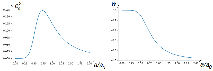
Figure 1: Graphs of $c_{s}^{2}(a)$ and $w(a)$ functions for Model 1 and parameter values $w_{0}=-0.7$ and $C=0.5$.

Let us further consider a concrete example:

$$f^{\prime}(w)=C\,,$$ (14)

where $C$ is a constant, such that $0<C<1$. Then it follows

$$f(w)-f(w_{0})=C(w-w_{0})\,,$$ (15)

which, using (10), leads to

$$w=w_{0}+\frac{1}{2C}\ln\frac{X}{X_{0}}\,.$$ (16)

Further

$$\int_{w_{0}}^{w}\frac{f^{\prime}(w^{\prime})}{w^{\prime}}d\,w^{\prime}=C\ln\frac{w}{w_{0}}\,,$$ (17)

which finally leads to

$$F=F_{0}\left(\frac{X}{X_{0}}\right)^{1/2}\left[\ 1+\frac{1}{2Cw_{0}}\ln\frac{X}{X_{0}}\right]^{C}\,.$$ (18)

The speed of sound squared is then from (21)

$$c_{s}^{2}=-\frac{C(1+w)w}{1-C(1+w)}\,,$$ (19)

and the dynamics of $w(a)$ is implicitly defined by

$$\left(\frac{w}{w_{0}}\right)^{C-1}\frac{w+1}{w_{0}+1}=\left(\frac{a}{a_{0}}\right)^{-3}\,.$$ (20)

3.2 Model 2

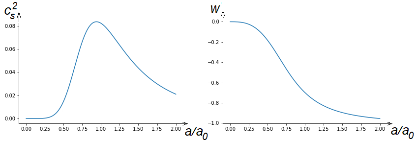
Figure 2: Graphs of $c_{s}^{2}(a)$ and $w(a)$ functions for Model 2 and parameter values $w_{0}=-0.7$, $\mu=0.5$ and $\nu=1$.

Next we consider the following model:

$$f^{\prime}(w)=\mu(-w)^{\nu}\,.$$ (21)

From (21) one obtains

$$f(w)-f(w_{0})=-\frac{\mu}{\nu+1}\left[(-w)^{\nu+1}-(-w_{0})^{\nu+1}\right]\,,$$ (22)

which, combined with (10), results in

$$w=-\left[(-w_{0})^{\nu+1}-\frac{\nu+1}{2\mu}\ln\frac{X}{X_{0}}\right]^{\frac{1}{\nu+1}}\,.$$ (23)

The required integral is then

$$\int_{w_{0}}^{w}\frac{f^{\prime}(w^{\prime})}{w^{\prime}}d\,w^{\prime}=\frac{\mu}{\nu}\left[(-w)^{\nu}-(-w_{0})^{\nu}\right]\,,$$ (24)

which results in the explicit expression for $F(X)$, i.e.

$$F=F_{0}\left(\frac{X}{X_{0}}\right)^{1/2}e^{\frac{\mu}{\nu}\left[\left[(-w_{0})^{\nu+1}-\frac{\nu+1}{2\mu}\ln\frac{X}{X_{0}}\right]^{\frac{\nu}{\nu+1}}-(-w_{0})^{\nu}\right]}\,.$$ (25)

The speed of sound squared follows from (21)

$$c_{s}^{2}=\mu\frac{(1+w)(-w)^{\nu+1}}{1-\mu(1+w)(-w)^{\nu}}\,,$$ (26)

whereas the dependence of $w$ on $a$ is given in an implicit form by

$$\frac{w_{0}}{w}\frac{w+1}{w_{0}+1}e^{\frac{\mu}{\nu}\left[(-w)^{\nu}-(-w_{0})^{\nu}\right]}=\left(\frac{a}{a_{0}}\right)^{-3}\,.$$ (27)

3.3 Model 3

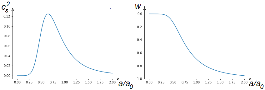
Figure 3: Graphs of $c_{s}^{2}(a)$ and $w(a)$ functions for Model 3 and parameter values $w_{0}=-0.7$ and $A=0.5$.

The following model that we consider is defined by

$$f^{\prime}(w)=A\sqrt{1+w}\,,$$ (28)

where $A$ is a constant. This model is well defined only if $w\geq-1$ throughout the entire cosmic timeline. It is further straightforward to obtain

$$f(w)-f(w_{0})=\frac{2A}{3}\left[(1+w)^{\frac{3}{2}}-(1+w_{0})^{\frac{3}{2}}\right]\,,$$ (29)

which, using (10), gives the expression for $w$ as a function of $X$

$$w=-1+\left[(1+w_{0})^{\frac{3}{2}}+\frac{3}{4A}\ln\frac{X}{X_{0}}\right]^{\frac{2}{3}}\,.$$ (30)

The integral needed for the reconstruction of the $F(X)$ function is then

$$\int_{w_{0}}^{w}\frac{f^{\prime}(w^{\prime})}{w^{\prime}}d\,w^{\prime}=2A(\sqrt{1+w}-\sqrt{1+w_{0}})+A\ln\left[\frac{(\sqrt{1+w}-1)(\sqrt{1+w_{0}}+1)}{(\sqrt{1+w}+1)(\sqrt{1+w_{0}}-1)}\right]\,,$$ (31)

which results in the expression

$$F = F_{0}\left(\frac{X}{X_{0}}\right)^{1/2}\left[\frac{\sqrt{1+w_{0}}+1}{\sqrt{1+w_{0}}-1}\frac{\left[(1+w_{0})^{\frac{3}{2}}+\frac{3}{4A}\ln\frac{X}{X_{0}}\right]^{\frac{1}{3}}-1}{\left[(1+w_{0})^{\frac{3}{2}}+\frac{3}{4A}\ln\frac{X}{X_{0}}\right]^{\frac{1}{3}}+1}\right]^{A}$$ (32)

$$\times e^{2A\left[\left[(1+w_{0})^{\frac{3}{2}}+\frac{3}{4A}\ln\frac{X}{X_{0}}\right]^{\frac{1}{3}}-\sqrt{1+w_{0}}\right]}\,.$$ (33)

Starting from (28), the speed of sound squared is

$$c_{s}^{2}=-\frac{Aw(1+w)^{\frac{3}{2}}}{1-A(1+w)^{\frac{3}{2}}}\,,$$ (34)

and the implicitly defined function $w(a)$ is then

$$\frac{w_{0}}{w}\frac{w+1}{w_{0}+1}\left[\frac{(\sqrt{1+w}-1)(\sqrt{1+w_{0}}+1)}{(\sqrt{1+w}+1)(\sqrt{1+w_{0}}-1)}\right]^{A}e^{2A\left(\sqrt{1+w}-\sqrt{1+w_{0}}\right)}=\left(\frac{a}{a_{0}}\right)^{-3}\,.$$ (35)

3.4 Model 4

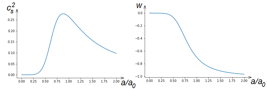
Figure 4: Graphs of $c_{s}^{2}(a)$ and $w(a)$ functions for Model 4 and parameter values $w_{0}=-0.7$ and $A=0.5$.

Another analytically tractable model follows from

$$f^{\prime}(w)=\frac{A}{\sqrt{1+w}}\,,$$ (36)

where $A$ is a constant. Like in the case of Model 3, this model is well defined only if $w\geq-1$ for all scale factor values. The form of $f(w)$ function is then

$$f(w)-f(w_{0})=2A\left[\sqrt{1+w}-\sqrt{1+w_{0}}\right]\,,$$ (37)

which, using (10), results in

$$w=-1+\left[\sqrt{1+w_{0}}+\frac{1}{4A}\ln\frac{X}{X_{0}}\right]^{2}\,.$$ (38)

The integration of $f(w)/w$ gives

$$\int_{w_{0}}^{w}\frac{f^{\prime}(w^{\prime})}{w^{\prime}}d\,w^{\prime}=A\ln\left[\frac{(\sqrt{1+w}-1)(\sqrt{1+w_{0}}+1)}{(\sqrt{1+w}+1)(\sqrt{1+w_{0}}-1)}\right]\,,$$ (39)

leading to

$$F=F_{0}\left(\frac{X}{X_{0}}\right)^{1/2}\left[\frac{1+\frac{1}{4A(\sqrt{1+w_{0}}-1)}\ln\frac{X}{X_{0}}}{1+\frac{1}{4A(\sqrt{1+w_{0}}+1)}\ln\frac{X}{X_{0}}}\right]^{A}\,.$$ (40)

The speed of sound squared is then obtained from (36)

$$c_{s}^{2}=-\frac{Aw\sqrt{1+w}}{1-A\sqrt{1+w}}\,,$$ (41)

and the dynamics of $w(a)$ acquires the following implicit form

$$\frac{w_{0}}{w}\frac{w+1}{w_{0}+1}\left[\frac{(\sqrt{1+w}-1)(\sqrt{1+w_{0}}+1)}{(\sqrt{1+w}+1)(\sqrt{1+w_{0}}-1)}\right]^{A}=\left(\frac{a}{a_{0}}\right)^{-3}\,.$$ (42)

3.5 Model 5

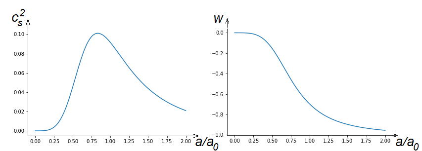
Figure 5: Graphs of $c_{s}^{2}(a)$ and $w(a)$ functions for Model 5 and parameter values $w_{0}=-0.7$, $A=0.5$ and $w_{*}=-2$.

Finally we consider a model defined by

$$f^{\prime}(w)=\frac{A}{w-w_{*}}\,,$$ (43)

where $A$ and $w_{*}$ are constants. Let us further assume that $w_{*}\neq-1$ and $A\neq w_{*}$. One obtains

$$f(w)-f(w_{0})=A\ln\frac{w-w_{*}}{w_{0}-w_{*}}\,,$$ (44)

which, using (10), results in

$$w=w_{*}+(w_{0}-w_{*})\left(\frac{X}{X_{0}}\right)^{\frac{1}{2A}}\,.$$ (45)

Further it is straightforward to obtain

$$\int_{w_{0}}^{w}\frac{f^{\prime}(w^{\prime})}{w^{\prime}}d\,w^{\prime}=\frac{A}{w_{*}}\left[\ln\frac{w-w_{*}}{w_{0}-w_{*}}-\ln\frac{w}{w_{0}}\right]\,,$$ (46)

which finally gives and expression

$$F=F_{0}\frac{\left(\frac{X}{X_{0}}\right)^{\frac{1}{2}\left(1+\frac{1}{w_{*}}\right)}}{\left[\frac{w_{*}}{w_{0}}+\left(1-\frac{w_{*}}{w_{0}}\right)\left(\frac{X}{X_{0}}\right)^{\frac{1}{2A}}\right]^{\frac{A}{w_{*}}}}\,.$$ (47)

Using (21), the speed of sound squared is

$$c_{s}^{2}=-\frac{Aw(1+w)}{w-w_{*}-A(1+w)}\,,$$ (48)

and the implicitly defined function $w(a)$ is

$$\left(\frac{w}{w_{0}}\right)^{-1-\frac{A}{w_{*}}}\frac{w+1}{w_{0}+1}\left(\frac{w-w_{*}}{w_{0}-w_{*}}\right)^{\frac{A}{w_{*}}}=\left(\frac{a}{a_{0}}\right)^{-3}\,.$$ (49)

The evolution of $w(a)$ depends on the concrete value of the $w_{*}$ parameter. For $-1<w_{0}<0$, and a sufficiently small postive $A$, if $w_{*}<-1$, the $w(a)$ function interpolates between 0 and -1. If $-1<w_{*}<w_{0}$, $w(a)$ is contained between 0 and $w_{*}$.

4 Discussion and conclusions

The focus of this paper is on the introduced method of purely kinetic k-essence model reconstruction for $c_{s}^{2}(w)$ models. The said reconstruction is explicitly analytically performed for five $c_{s}^{2}(w)$ models. The introduced method is, therefore, an alternative to approach where $c_{s}^{2}$ is modeled directly as a function of $w$, which was elaborated in [40].

The considered models (models 1, 2, 3, 4 and 5) were chosen on the basis of analytical tractability of required calculations. However, for all of them there are parameter regimes where they represent a cosmic component corresponding to dark matter - dark energy unification. The dependence of $c_{s}^{2}$ and $w$ on the scale factor $a$ are presented in Fig. 1 for Model 1, Fig. 2 for Model 2, Fig. 3 for Model 3, Fig. 4 for Model 4 and Fig. 5 for Model 5. In all figures $w$ vanishes for small $a$ and approaches -1 for large values of $a$, whereas $c_{s}^{2}$ vanishes for small and large values of the scale factor and reaches maximum at some intermediate scale factor value. The deviation of the speed of sound squared from 0 is controlled by one of model parameters which suggests that models might be consistent with growth of structure data for sufficiently small values of corresponding parameters. This claim can be fully statistically verified only by the model comparison with the real cosmological observations, which is out of scope of this paper. Furthermore, all parametric regimes of the constructed models have not been thoroughly examined because it would exceed the scope of this paper. It is certain that there is a number of additional parameter regimes, which were not presented here, that may be of interest. In conclusion, although the considered models were chosen to demonstrate the introduced reconstruction method, they are, in adequate parameter regime, also interesting as possible explanations of the cosmic dark sector.

Availability and straightforwardness of solutions to the above models depends crucially on the integrability and invertibility of functions used in the reconstruction method. With a careful approach, it is possible to find a number of functions $f(w)$ that can satisfy these conditions.

As already discussed in [40], even if $f(w)$ function is not analytically invertible, one may obtain parametric solutions $(X(w),F(w))$, which can be used to obtain parametric plots of $F(X)$. Furthermore, since there are parameter regimes in which $w$ is constrained to a $[-1,0]$ interval, a numerical analysis of such parametric solutions is simplified.

In conclusion, the introduced method allows analytical reconstruction of an equivalent purely kinetic k-essence description of a broad class of $c_{s}^{2}(w)$ models. The method is demonstrated on five $c_{s}^{2}(w)$ models. The analyzed models can be useful in the study of dak matter - dark energy unified dark sector in appropriate parameter regimes.

References

- [1] A. G. Riess et al., Astron. J. 116 (1998) 1009.
- [2] S. Perlmutter et al., Astrophys. J. 517 (1999) 565.
- [3] P. A. R. Ade et al. (Planck) Astron. Astrophys. 594 (2016) A13.
- [4] E. Komatsu et al, Prog. Theor. Exp. Phys. 6 (2014) 06B102.
- [5] C. Alcock et al., Phys. Rev. Lett. 74 (1995) 2867.
- [6] D. Huterer, D. L. Shafer, Rept. Prog. Phys. 81 (2018) 016901.
- [7] P. Brax, Rept. Prog. Phys. 81 (2018) 016902.
- [8] E. J. Copeland, M. Sami, S. Tsujikawa, Int. J. Mod. Phys. D15 (2006) 1753.
- [9] J. Frieman, M. Turner, D. Huterer, Ann. Rev. Astron. Astrophys. 46 (2008) 385.
- [10] K. Bamba, S. Capozziello, S. Nojiri, S. D. Odintsov, Astrophys. Space Sci. 342 (2012) 155.
- [11] S. Nojiri, S.D. Odintsov, V.K. Oikonomou, Phys. Rept. 692 (2017) 1.
- [12] A. De Felice, S. Tsujikawa, Living Rev.Rel. 13 (2010) 3.
- [13] T. P. Sotiriou, V. Faraoni, Rev. Mod. Phys. 82 (2010) 451.
- [14] S. Tulin, H.-B. Yu, Phys. Rept. 730 (2018) 1.
- [15] M. Klasen, M. Pohl, G. Sigl, Prog. Part. Nucl. Phys. 85 (2015) 1.
- [16] G. Bertone, D. Hooper, Rev. Mod. Phys. 90 (2018) 045002.
- [17] R. Barkana, Nature 555 (2018) 71.
- [18] M. Milgrom, Astrophys. J 270 (1983) 371.
- [19] D. V. Bugg, Can. J. Phys. 93 (2015) 119.
- [20] S. McGaugh, F. Lelli, J. Schombert, Phys. Rev. Lett. 117 (2016) 201101.
- [21] C. Skordis, T. Zlosnik, Phys. Rev. Lett. 127 (2021) 161302.
- [22] S. Vagnozzi, Class. Quant. Grav. 34 (2017) 185006.
- [23] E. Di Valentino et al., Astropart. Phys. 131 (2021) 102605.
- [24] E. Di Valentino, O. Mena, S. Pan, L. Visinelli, W. Yang, A. Melchiorri, D. F. Mota, A. G. Riess, J. Silk, Class. Quantum Grav. 38 (2021) 153001.
- [25] E. Abdalla et al., J. High En. Astrophys. 2204 (2022) 002.
- [26] S. Vagnozzi, Phys. Rev. D 102 (2020) 023518.
- [27] D. Bertacca, N. Bartolo, S. Matarrese, Adv. Astron. 2010 (2010) 904379.
- [28] E. V. Linder, R. J. Scherrer, Phys. Rev. D 80 (2009) 023008.
- [29] A.Y. Kamenshchik, U. Moschella, V. Pasquier, Phys. Lett. B 511 (2001) 265.
- [30] N. Bilic, G. B. Tupper, R. D. Viollier, Phys. Lett. B 535 (2002) 17.
- [31] M. C. Bento, O. Bertolami, A. A. Sen, Phys. Rev. D 66 (2002), 043507.
- [32] J. D. Barrow, Nucl. Phys. B 310 (1988) 743.
- [33] H. B. Benaoum, arXiv:hep-th/0205140v1.
- [34] N. Bilic, G. B. Tupper, R. D. Viollier, JCAP 0510 (2005) 003.
- [35] R. Lazkoz, M. Ortiz-Baños, V. Salzano, Phys. Dark Univ. 24 (2019) 100279.
- [36] H. Sandvik, M. Tegmark, M. Zaldarriaga, I. Waga, Phys. Rev. D 69 (2004) 123524.
- [37] W. J. Wolf, P. G. Ferreira, Phys. Rev. D 108 (2023) 103519.
- [38] N. Caplar, H. Stefancic, Phys. Rev. D 87 (2013) 023510.
- [39] D. Perkovic, H. Stefancic, Phys. Lett. B 797 (2019) 134806.
- [40] D. Perkovic, H. Stefancic, Phys. Dark Univ. 32 (2021) 100827.
- [41] D. Perkovic, H. Stefancic, Int. J. Mod. Phys. D 28 (2018) 1950045.
- [42] D. Perkovic, H. Stefancic, Eur. Phys. J. C 80 (2020) 629.
- [43] D. Perkovic, H. Stefancic, Eur. Phys. J. C 83 (2023) 306.
- [44] C. Armendariz-Picon, T. Damour, V. F. Mukhanov, Phys. Lett. B 458 (1999) 209.
- [45] J. Garriga, V. F. Mukhanov, Phys. Lett. B 458 (1999) 219.
- [46] T. Chiba, T. Okabe, M. Yamaguchi, Phys. Rev. D 62 (2000) 023511.
- [47] C. Armendariz-Picon, V. F. Mukhanov, P. J. Steinhardt, Phys. Rev. Lett. 85 (2000) 4438.
- [48] C. Armendariz-Picon, V. F. Mukhanov, P. J. Steinhardt, Phys. Rev. D 63 (2001) 103510.
- [49] M Malquarti, E. J. Copeland, A. R. Liddle, M. Trodden, Phys. Rev. D 67 (2003) 123503.
- [50] M. Malquarti, E. J. Copeland, A. R. Liddle, Phys. Rev. D 68 (2003) 023512.
- [51] L. P. Chimento, A. Feinstein, Mod. Phys. Lett. A 19 (2004) 761.
- [52] R. de Putter, E. V. Linder, Astropart. Phys. 28 (2007) 263.
- [53] R. J. Scherrer, Phys. Rev. Lett. 93 (2004) 011301.
- [54] L. P. Chimento, M. I. Forte, R. Lazkoz, Mod. Phys. Lett.A 20 (2005) 2075.
- [55] C. Armendariz-Picon, E. A. Lim, JCAP 08 (2005) 007.
- [56] D. Bertacca, S. Matarrese, M. Pietroni, Mod. Phys. Lett. A 22 (2007) 2893.
- [57] D. Bertacca, N. Bartolo, A. Diaferio, S. Matarrese, JCAP 10 (2008) 023.
- [58] N. Bilic, G. B. Tupper, R. D. Viollier, Phys. Rev. D 80 (2009) 023515.
- [59] O. F. Piattella, D. Bertacca, M. Bruni, D. Pietrobon, JCAP 01 (2010) 014.
- [60] A. Sen, JHEP 04 (2002) 048.
- [61] A. Sen, Mod. Phys. Lett. A 17 (2002) 1797.
- [62] G. W. Gibbons, Phys. Lett. B 537 (2002) 1.
- [63] J. S. Bagla, H. K. Jassal, T. Padmanabhan, Phys. Rev. D 67 (2003) 063504.
- [64] A. Diez-Tejedor, A. Feinstein, Int. J. Mod. Phys. D 14 (2005) 1561.
- [65] F. Arroja, M. Sasaki, Phys. Rev. D 81 (2010) 107301.
- [66] V. M. C. Ferreira, P. P. Avelino, R. P. L. Azevedo, Phys. Rev. D 102 (2020) 063525.