Applications of Dual Complex Adjoint Matrix in Eigenvalue Computation of Dual Quaternion Hermitian Matrix

Abstract

Dual quaternions and dual quaternion matrices have found widespread applications in robotic research, with their spectral theory been extensively studied in recent years. This paper delves into the realm of eigenvalue computation and related problems specific to dual quaternion Hermitian matrices. We establish the connection between dual quaternion matrices and their dual complex adjoint matrices, concerning eigenvalue problems and matrix rank-k approximations. By integrating the dual complex adjoint matrix, we refine the power method for eigenvalue computation for dual quaternion Hermitian matrices, achieving greater numerical efficiency. Furthermore, leveraging the eigen-decomposition of dual complex adjoint matrices, we introduce a novel approach for calculating all eigenpairs of dual quaternion Hermitian matrices. This method surpasses the power method in terms of accuracy and speed and addresses its limitations, as exemplified by its application to the eigenvalue computation of Laplacian matrices, where our algorithm demonstrates significant advantages. Additionally, we apply the improved power method and optimal rank-k approximations to pose graph optimization problem, enhancing efficiency and success rates, especially under low observation conditions.

1 Introduction

Dual quaternions and dual quaternion matrices exhibit a vast array of applications in robotics research, encompassing problems such as Hand-Eye calibration problem [8], simultaneous localization and mapping (SLAM) problem [1, 2, 3, 6, 18, 19], and multi-agent formation control [15]. Dual quaternion Hermitian matrices, a vital subclass of dual quaternion matrices, possess admirable properties that are instrumental in analyzing the stability of multi-agent formation control systems [15] and solving pose graph optimization (PGO) problems [3, 5, 10].

Scholars have delved deeply into the theory of dual quaternion matrices. Qi and Luo [13] investigated the spectral theory, revealing that if a right eigenvalue of a dual quaternion matrix is a dual number, it is concurrently a left eigenvalue, referred to simply as an eigenvalue of the matrix. Notably, an n-dimensional dual quaternion Hermitian matrix possesses exactly n eigenvalues, all of which are dual numbers. Leveraging this property, they derived the eigenvalue decomposition for such matrices. Further, Ling et al. [12] explored the minimax principle for dual quaternion Hermitian matrices and extended the Fan-Hoffman inequality to the domain of dual quaternion matrices. The von Neumann-type trace inequality for dual quaternion matrices and Hoffman-Wielandt-type inequality for dual quaternion Hermitian matrices were studied in a subsequent work [11].

Cui and Qi [5] introduced a power method for computing the strict dominant eigenvalues of dual quaternion Hermitian matrices. An eigenvalue $\hat{\lambda}$ is called the strict dominant eigenvalue of a dual quaternion Hermitian matrix $\hat{\mathbf{Q}}$ with multiplicity $k$, if $\hat{\mathbf{Q}}$ possesses $k$ identical eigenvalues equal to $\hat{\lambda}$, and the magnitude of the standard part of $\hat{\lambda}$ exceeds that of the remaining $n-k$ eigenvalues. It proves that the convergence rate of the power method for the strict dominant eigenpairs of dual quaternion Hermitian matrices is linear. Nevertheless, the power method has its limitations. As evidenced by the numerical experiments in [5], the computation time significantly increases with the matrix dimension. Furthermore, when the dual quaternion Hermitian matrix has two eigenvalues with identical standard parts but different dual parts, the power method may be invalid to calculate these eigenvalues. Thus, there is a pressing need for more efficient algorithms to compute the eigenvalues of dual quaternion Hermitian matrices that can overcome the shortcomings of the power method.

The complex adjoint matrix has played a pivotal role in studying quaternion matrix theory [20], transforming the eigenvalue problem of quaternion matrices into one for complex matrices with special structures. Given the exhaustive research on complex matrix eigenvalue theory, the properties of the complex adjoint matrix simplify quaternion eigenvalue investigations. Inspired by these insights, our work in paper [7] introduces the dual complex adjoint matrix tailored for dual quaternion matrices, delving into its properties. Based on these properties, we define and prove the uniqueness of the standard right eigenvalues of dual quaternion matrices, and provide explicit solutions to Hand-Eye calibration problems. Furthermore, we reframe dual quaternion linear equation systems as dual complex counterparts, refining the Rayleigh quotient iteration method and bolstering computational performance. Consequently, the dual complex adjoint matrix emerges as a versatile tool with broad applications in dual quaternion matrix theory. In this paper, we aim to uncover the relationship between dual complex adjoint matrices and dual quaternion matrices, concerning eigenvalue problems and matrix rank-k approximations.

The structure of this paper is organized as follows. Section 2 introduces fundamental knowledge of dual quaternion matrices and its eigenvalue theory. Section 3 explores the connection between dual complex adjoint matrices and dual quaternion matrices in eigenvalue problems and optimal rank-k approximations. It introduces a novel approach to compute all eigenpairs of dual quaternion Hermitian matrices, leveraging the eigen-decomposition of the dual complex adjoint matrix. Furthermore, a hybrid algorithm integrating the dual complex adjoint matrix with the power method is devised. Section 4 presents numerical experiments applying our algorithms to solve eigenvalue problems for Laplacian matrices and pose graph optimization problems. Some final remarks are drawn in Section 5.

2 Preliminary

In this section, we introduce some preliminary knowledge about the dual number, dual complex number, quaternion, dual quaternion, dual quaternion matrix, and the eigenvalue theory of dual quaternion matrix.

2.1 Dual quaternion

Denote $\mathbb{R}$, $\mathbb{C}$, $\mathbb{D}$, $\mathbb{DC}$, $\mathbb{Q}$, $\mathbb{U}$, $\hat{\mathbb{Q}}$ and $\hat{\mathbb{U}}$ as the set of real numbers, complex numbers, dual numbers, dual complex numbers, quaternions, unit quaternions, dual quaternions, and unit dual quaternions, respectively.

The symbol $\varepsilon$ is denoted as the infinitesimal unit, satisfies $\varepsilon\neq 0$ and $\varepsilon^{2}=0$. $\varepsilon$ is commutative with real numbers and quaternions.

2.1.1 Dual number and dual complex number

Definition 2.1.

A dual complex number $\hat{a}=a_{st}+a_{\mathcal{I}}\varepsilon\in\mathbb{DC}$ has standard part $a_{st}\in\mathbb{C}$ and dual part $a_{\mathcal{I}}\in\mathbb{C}$. We say that $\hat{a}$ is appreciable if $a_{st}\neq 0$. If $a_{st},a_{\mathcal{I}}\in\mathbb{R}$, then $\hat{a}$ is called a dual number.

The following definition lists some operators about dual complex numbers, which can be found in [14].

Definition 2.2.

Let $\hat{a}=a_{st}+a_{\mathcal{I}}\varepsilon$ and $\hat{b}=b_{st}+b_{\mathcal{I}}\varepsilon$ be any two dual complex numbers. The conjugate, absolute value of $\hat{a}$, and the addition, multiplication, division between $\hat{a}$ and $\hat{b}$ are defined as follows.

• The conjugate of $\hat{a}$ is $\hat{a}^{\ast}=a_{st}^{\ast}+a_{\mathcal{I}}^{\ast}\varepsilon,$ where $a_{st}^{\ast}$ and $a_{\mathcal{I}}^{\ast}$ are conjugates of the complex numbers $a_{st}$ and $a_{\mathcal{I}}$, respectively.

• The addition and multiplication of $\hat{a}$ and $\hat{b}$ are

  $$\hat{a}+\hat{b}=\hat{b}+\hat{a}=\left(a_{st}+b_{st}\right)+\left(a_{\mathcal{I}}+b_{\mathcal{I}}\right)\varepsilon,$$

  and

  $$\hat{a}\hat{b}=\hat{b}\hat{a}=a_{st}b_{st}+\left(a_{st}b_{\mathcal{I}}+a_{\mathcal{I}}b_{st}\right)\varepsilon.$$

• When $b_{st}\neq 0$ or $a_{st}=b_{st}=0$, we can define the division operation of dual numbers as

  $$\frac{\hat{a}}{\hat{b}}=\begin{cases}\dfrac{a_{st}}{b_{st}}+\left(\dfrac{a_{\mathcal{I}}}{b_{st}}-\dfrac{a_{st}b_{\mathcal{I}}}{b_{st}b_{st}}\right)\varepsilon,&{\rm if}\quad b_{st}\neq 0,\\ \dfrac{a_{\mathcal{I}}}{b_{\mathcal{I}}}+c\varepsilon,&{\rm if}\quad a_{st}=b_{st}=0,\end{cases}$$

  where $c$ is an arbitrary complex number.

• The absolute value of $\hat{a}$ is

  $$\left|\hat{a}\right|=\begin{cases}\left|a_{st}\right|+{\rm sgn}(a_{st})a_{\mathcal{I}}\varepsilon,&{\rm if}\quad a_{st}\neq 0,\\ \left|a_{\mathcal{I}}\right|\varepsilon,&\text{\rm otherwise.}\end{cases}$$

The order operation for dual numbers was defined in [5] and the limit operation to dual number sequences was defined in [14].

Definition 2.3.

Let $\hat{a}=a_{st}+a_{\mathcal{I}}\varepsilon$, $\hat{b}=b_{st}+b_{\mathcal{I}}\varepsilon$ be any two dual numbers and $\left\{\hat{a}_{k}=a_{k,st}+a_{k,\mathcal{I}}\varepsilon:k=1,2,\cdots\right\}$ be a dual number sequence. We give the order operation between $\hat{a}$ and $\hat{b}$, and extend limit operation to dual number sequences.

• We say that $\hat{a}>\hat{b}$ if

  $$\text{$a_{st}>b_{st}$ ~{}~{}~{}{\rm or}~{}~{}~{} $a_{st}=b_{st}$ {\rm and} $a_{\mathcal{I}}>b_{\mathcal{I}}$}.$$

• We say that $\left\{\hat{a}_{k}=a_{k,st}+a_{k,\mathcal{I}}\varepsilon\right\}$ converges to a limit $\hat{a}=a_{st}+a_{\mathcal{I}}\varepsilon$ if

  $$\underset{k\rightarrow\infty}{\lim}a_{k,st}=a_{st}\quad{\rm and}\quad\underset{k\rightarrow\infty}{\lim}a_{k,\mathcal{I}}=a_{\mathcal{I}}.$$

Similar to the equivalent infinity symbol $O$ of real numbers, we introduce a notation for the equivalent infinity of dual numbers as follows [5].

Definition 2.4.

Let $\{\hat{a}_{k}=a_{k,st}+a_{k,\mathcal{I}}\varepsilon:k=1,2,\cdots\}\subset\mathbb{D}$ be a dual number sequence and $\{b_{k}:k=1,2,\cdots\}\subset\mathbb{R}$ is a real number sequence. We denote $\hat{a}_{k}=O_{D}(b_{k})$ if $a_{k,st}=O(b_{k})$ and $a_{k,\mathcal{I}}=O(b_{k})$. Furthermore, if there exist a constant $0<c<1$ and a polynomial $h(k)$, such that $\hat{a}_{k}=O_{D}(c^{k}h(k))$, then we write $\hat{a}_{k}=\tilde{O}_{D}(c^{k})$.

2.1.2 Quaternion

Definition 2.5.

A quaternion can be represented as $\tilde{q}=q_{0}+q_{1}i+q_{2}j+q_{3}k$, where $q_{0},q_{1},q_{2},q_{3}$ are real numbers, $i,j,k$ satisfy $ij=k$, $jk=i$,$ki=j$ and $i^{2}=j^{2}=k^{2}=-1$. $\tilde{q}$ can also be represented as $\tilde{q}=\left[q_{0},q_{1},q_{2},q_{3}\right]$, which is a real four-dimensional vector. We can rewrite $\tilde{q}=[q_{0},\vec{q}]$, where $\vec{q}$ is a real three-dimensional vector [4, 8, 18].

Denote $\tilde{1}=\left[1,0,0,0\right]\in\mathbb{Q}$ and $\tilde{0}=\left[0,0,0,0\right]\in\mathbb{Q}$ as the identity element and zero element of the quaternion set $\mathbb{Q}$.

The following definition lists some operators about quaternions.

Definition 2.6.

Let $\tilde{p}=\left[p_{0},\vec{p}\right]$ and $\tilde{q}=\left[q_{0},\vec{q}\right]$ be any two quaternions. The conjugate, magnitude, and inverse of $\tilde{p}$, and the addition, multiplication between $\tilde{q}$ and $\tilde{p}$ are defined as follows.

• The conjugate of $\tilde{p}$ is $\tilde{p}^{\ast}=\left[p_{0},-\vec{p}\right]$.

• The magnitude of $\tilde{p}$ is $\left|\tilde{p}\right|=\sqrt{p_{0}^{2}+\left\|\vec{p}\right\|_{2}^{2}}$. If $\left|\tilde{p}\right|=1$, then we say that $\tilde{p}\in\mathbb{U}$ is a unit quaternion.

• The addition and multiplicity of $\tilde{q}$ and $\tilde{p}$ are

  $$\tilde{p}+\tilde{q}=\tilde{q}+\tilde{p}=\left[p_{0}+q_{0},\vec{p}+\vec{q}\right]$$ (1)

  and

  $$\tilde{p}\tilde{q}=\left[p_{0}q_{0}-\vec{p}\cdot\vec{q},p_{0}\vec{q}+q_{0}\vec{p}+\vec{p}\times\vec{q}\right].$$ (2)

• If $\tilde{q}\tilde{p}=\tilde{p}\tilde{q}=\tilde{1}$, then we call the quaternion $\tilde{p}$ is invertible and the inverse of $\tilde{p}$ is $\tilde{p}^{-1}=\tilde{q}$. If $\tilde{p}\in\mathbb{U}$, we have $\tilde{p}^{\ast}\tilde{p}=\tilde{p}\tilde{p}^{\ast}=\tilde{1}$, i.e., $\tilde{p}$ is invertible and $\tilde{p}^{-1}=\tilde{p}^{\ast}$. Generally, if quaternion $\tilde{p}\neq\tilde{0}$, we have $\frac{\tilde{p}^{\ast}}{|\tilde{p}|^{2}}\tilde{p}=\tilde{p}\frac{\tilde{p}^{\ast}}{|\tilde{p}|^{2}}=\tilde{1}$, then $\tilde{p}^{-1}=\frac{\tilde{p}^{\ast}}{|\tilde{p}|^{2}}$.

2.1.3 Dual quaternion

Definition 2.7.

A dual quaternion $\hat{p}=\tilde{p}_{st}+\tilde{p}_{\mathcal{I}}\varepsilon\in\hat{\mathbb{Q}}$ has standard part $\tilde{p}_{st}\in\mathbb{Q}$ and dual part $\tilde{p}_{\mathcal{I}}\in\mathbb{Q}$. We say that $\hat{q}$ is appreciable if $\tilde{p}_{st}\neq\tilde{0}$.

Denote $\hat{1}=\tilde{1}+\tilde{0}\varepsilon\in\hat{\mathbb{Q}}$ and $\tilde{0}=\tilde{0}+\tilde{0}\varepsilon\in\hat{\mathbb{Q}}$ as the identity element and zero element of the dual quaternion set $\hat{\mathbb{Q}}$.

The following definition lists some operators about dual quaternions.

Definition 2.8.

Let $\hat{p}=\tilde{p}_{st}+\tilde{p}_{\mathcal{I}}\varepsilon$ and $\hat{q}=\tilde{q}_{st}+\tilde{q}_{\mathcal{I}}\varepsilon$ be dual quaternions. The conjugation, absolute value and magnitude of $\hat{p}$ and the addition, multiplicity and division of $\hat{p}$ and $\hat{q}$ are defined as follows.

• The conjugate of $\hat{p}$ is $\hat{p}^{\ast}=\tilde{p}_{st}^{\ast}+\tilde{p}_{\mathcal{I}}^{\ast}\varepsilon$, where $\tilde{p}_{st}^{\ast}$ and $\tilde{p}_{\mathcal{I}}^{\ast}$ are the conjugate of quaternions.

• The absolute value [14] of $\hat{p}$ is

  $$\left|\hat{p}\right|=\begin{cases}\left|\tilde{p}_{st}\right|+\frac{sc(\tilde{p}_{st}^{\ast}\tilde{p}_{\mathcal{I}})}{\left|\tilde{p}_{st}\right|}\varepsilon,&\text{if}\quad\tilde{p}_{st}\neq\tilde{0},\\ \left|\tilde{p}_{\mathcal{I}}\right|\varepsilon,&\text{if}\quad\tilde{p}_{st}=\tilde{0},\end{cases}$$ (3)

  where $sc(\tilde{p})=\frac{1}{2}(\tilde{p}+\tilde{p}^{\ast})$. If $|\hat{p}|=\hat{1}$, then we say that $\hat{p}\in\hat{\mathbb{U}}$ is a unit dual quaternion.

• The magnitude of $\hat{p}$ is

  $$\left|\hat{p}\right|_{2}=\sqrt{|\tilde{p}_{st}|^{2}+|\tilde{p}_{\mathcal{I}}|^{2}}.$$ (4)

• The addition and multiplicity of $\hat{p}$ and $\hat{q}$ are

  $$\hat{p}+\hat{q}=\hat{q}+\hat{p}=\left(\tilde{p}_{st}+\tilde{q}_{st}\right)+\left(\tilde{p}_{\mathcal{I}}+\tilde{q}_{\mathcal{I}}\right)\varepsilon,$$ (5)

  and

  $$\hat{p}\hat{q}=\tilde{p}_{st}\tilde{q}_{st}+\left(\tilde{p}_{st}\tilde{q}_{\mathcal{I}}+\tilde{p}_{\mathcal{I}}\tilde{q}_{st}\right)\varepsilon.$$ (6)

• If $\tilde{q}_{st}\neq\tilde{0}$ or $\tilde{q}_{st}=\tilde{q}_{st}=\tilde{0}$, we can define the division of $\hat{p}$ and $\hat{q}$ as

  $$\frac{\tilde{p}_{st}+\tilde{p}_{\mathcal{I}}\varepsilon}{\tilde{q}_{st}+\tilde{q}_{\mathcal{I}}\varepsilon}=\begin{cases}\dfrac{\tilde{p}_{st}}{\tilde{q}_{st}}+\left(\dfrac{\tilde{p}_{\mathcal{I}}}{\tilde{q}_{st}}-\dfrac{\tilde{p}_{st}\tilde{q}_{\mathcal{I}}}{\tilde{q}_{st}\tilde{q}_{st}}\right)\varepsilon,&\text{if}\quad\tilde{q}_{st}\neq\tilde{0},\\ \dfrac{\tilde{p}_{\mathcal{I}}}{\tilde{q}_{\mathcal{I}}}+\tilde{c}\varepsilon,&\text{if}\quad\tilde{p}_{st}=\tilde{q}_{st}=\tilde{0},\end{cases}$$ (7)

  where $\tilde{c}$ is an arbitrary quaternion.

• If $\hat{q}\hat{p}=\hat{p}\hat{q}=\hat{1}$, then $\hat{p}$ is called invertible and the inverse of $\hat{p}$ is $\hat{p}^{-1}=\hat{q}$. If $\hat{p}\in\hat{\mathbb{U}}$, we have $\hat{p}^{\ast}\hat{p}=\hat{p}\hat{p}^{\ast}=\hat{1}$, i.e., $\hat{p}$ is invertible and $\hat{p}^{-1}=\hat{p}^{\ast}$. Generally, if $\hat{p}$ is appreciable, we have $\hat{p}^{-1}=\tilde{p}^{-1}_{st}-\tilde{p}^{-1}_{st}\tilde{p}_{\mathcal{I}}\tilde{p}^{-1}_{st}\varepsilon$.

A unit dual quaternion $\hat{u}$ is called the projection of $\hat{q}\in\hat{\mathbb{Q}}$ onto the set $\hat{\mathbb{U}}$, if

$$\hat{u}\in\underset{\hat{v}\in\hat{\mathbb{U}}}{\arg\min}~{}|\hat{v}-\hat{q}|^{2}.$$ (8)

The following lemma provides a feasible solution [5].

Lemma 1.

Suppose that $\hat{q}=\tilde{q}_{st}+\tilde{q}_{\mathcal{I}}\varepsilon\in\hat{\mathbb{Q}}$.

If $\tilde{q}_{st}\neq\tilde{0}$, denote $\hat{u}=\tilde{u}_{st}+\tilde{u}_{\mathcal{I}}\varepsilon\in\hat{\mathbb{U}}$ as the normalization of $\hat{q}$, i.e.,

$$\hat{u}=\frac{\hat{q}}{\left|\hat{q}\right|}=\frac{\tilde{q}_{st}}{\left|\tilde{q}_{st}\right|}+\left(\frac{\tilde{q}_{\mathcal{I}}}{\left|\tilde{q}_{st}\right|}-\frac{\tilde{q}_{st}}{\left|\tilde{q}_{st}\right|}sc\left(\frac{\tilde{q}_{st}^{\ast}}{\left|\tilde{q}_{st}\right|}\frac{\tilde{q}_{\mathcal{I}}}{\left|\tilde{q}_{st}\right|}\right)\right)\varepsilon,$$ (9)

then $\hat{u}$ is the projection of $\hat{q}$ onto the set $\hat{\mathbb{U}}$.

If $\tilde{q}_{st}=\tilde{0}$ and $\tilde{q}_{\mathcal{I}}\neq\tilde{0}$, then the projection of $\hat{q}$ onto the set $\hat{\mathbb{U}}$ is

$$\hat{u}=\frac{\tilde{q}_{\mathcal{I}}}{\left|\tilde{q}_{\mathcal{I}}\right|}+\tilde{c}\varepsilon\in\hat{\mathbb{U}},$$ (10)

where $\tilde{c}$ is an arbitrary quaternion, satisfies $sc(\tilde{q}_{\mathcal{I}}^{\ast}\tilde{c})=\tilde{0}$.

2.2 dual quaternion matrix

The sets of dual number matrix, dual complex matrix, quaternion matrix, dual quaternion matrix, and unit dual quaternion matrix with dimension $n\times m$ are denoted as $\mathbb{D}^{n\times m}$, $\mathbb{DC}^{n\times m}$, $\mathbb{Q}^{n\times m}$, $\hat{\mathbb{Q}}^{n\times m}$ and $\hat{\mathbb{U}}^{n\times m}$. Denote $O^{n\times m}$, $\hat{O}^{n\times m}$, $\tilde{\mathbf{O}}^{n\times m}$ and $\hat{\mathbf{O}}^{n\times m}$ as the zero element of the set of complex matrices, dual complex matrices, quaternion matrices and dual quaternion matrices with dimension $n\times m$, respectively. Denote $\hat{I}_{n}$, $\tilde{\mathbf{I}}_{n}$ and $\hat{\mathbf{I}}_{n}$ as the identity element of the set of dual complex matrices, quaternion matrices and dual quaternion matrices with dimension $n\times n$, respectively.

A quaternion matrix $\tilde{\mathbf{Q}}\in\mathbb{Q}^{m\times n}$ can be expressed as $\tilde{\mathbf{Q}}=Q_{1}+Q_{2}i+Q_{3}j+Q_{4}k\in\mathbb{Q}^{m\times n}$, where $Q_{1},Q_{2},Q_{3},Q_{4}\in\mathbb{R}^{m\times n}$. Denote $P_{1}=Q_{1}+Q_{2}i$ and $P_{2}=Q_{3}+Q_{4}i$, then we can rewrite $\tilde{\mathbf{Q}}$ as $\tilde{\mathbf{Q}}=P_{1}+P_{2}j$. The $F$-norm of quaternion matrix $\tilde{\mathbf{Q}}=(\tilde{q}_{ij})\in\tilde{\mathbb{Q}}^{m\times n}$ is defined as $\|\tilde{\mathbf{Q}}\|_{F}=\sqrt{\sum_{ij}|\tilde{q}_{ij}|^{2}}$. The magnitude of the quaternion vector $\tilde{\mathbf{x}}=(\tilde{x}_{i})\in\tilde{\mathbb{Q}}^{n\times 1}$ is defined as $\left\|\tilde{\mathbf{x}}\right\|=\sqrt{\sum_{i=1}^{n}|\tilde{x}_{i}|^{2}}$.

2.2.1 dual complex matrix

A dual complex matrix $\hat{P}=P_{st}+P_{\mathcal{I}}\varepsilon\in\mathbb{DC}^{n\times m}$ has standard part $P_{st}$ and dual part $P_{\mathcal{I}}$, where $P_{st},P_{\mathcal{I}}\in\mathbb{C}^{n\times m}$. If $P_{st}\neq O$, then the dual complex matrix $\hat{P}$ is called appreciable. The transpose and the conjugate of $\hat{P}=(\hat{p}_{ij})$ are $\hat{P}^{T}=(\hat{p}_{ji})$ and $\hat{P}^{\ast}=(\hat{p}_{ji}^{\ast})$, respectively. If $\hat{P}^{\ast}=\hat{P}$, then $\hat{P}$ is called a dual complex Hermitian matrix. A dual complex matrix $\hat{U}\in\mathbb{DC}^{n\times n}$ is a unitary matrix, if $\hat{U}^{\ast}\hat{U}=\hat{U}\hat{U}^{\ast}=\hat{I}_{n}$.

The 2-norm of dual complex vector $\hat{\mathbf{\mathbf{x}}}=\mathbf{x}_{st}+\mathbf{x}_{\mathcal{I}}\varepsilon=(\hat{x}_{i})\in\mathbb{DC}^{n\times 1}$ is defined as

$$\left\|\hat{\mathbf{x}}\right\|_{2}=\begin{cases}\sqrt{\sum_{i=1}^{n}\left|\hat{x}_{i}\right|^{2}},&\text{if}\quad\mathbf{x}_{st}\neq O,\\ \|\mathbf{x}_{\mathcal{I}}\|_{2}\varepsilon,&\text{if}\quad\mathbf{x}_{st}=O.\end{cases}$$ (11)

The following defines the eigenvalues and eigenvectors of dual complex matrices.

Definition 2.9.

Suppose that $\hat{P}\in\mathbb{DC}^{n\times n}$. If there exist $\hat{\lambda}\in\mathbb{DC}$ and appreciable dual complex vector $\hat{\mathbf{x}}\in\mathbb{DC}^{n\times 1}$ such that

$$\hat{P}\hat{\mathbf{x}}=\hat{\mathbf{x}}\hat{\lambda},$$ (12)

then $\hat{\lambda}$ and $\hat{\mathbf{x}}$ are eigenvalue and corresponding eigenvector of $\hat{P}$.

Specifically, the dual complex Hermitian matrix with dimension $n$ has exactly $n$ dual number eigenvalues.

The $F$-norm and the $F^{*}$-norm of dual complex matrices are defined as follows.

Definition 2.10.

Suppose that $\hat{P}=P_{1}+P_{2}\varepsilon\in\mathbb{DC}^{n\times m}$, the $F$-norm and the $F^{*}$-norm of $\hat{P}$ are

$$\|\hat{P}\|_{F}=\begin{cases}\left\|P_{1}\right\|_{F}+\frac{sc(tr(P_{1}^{\ast}P_{2}))}{\left\|P_{1}\right\|_{F}}\varepsilon,&\text{if}\quad P_{1}\neq O,\\ \left\|P_{2}\right\|_{F}\varepsilon,&\text{if}\quad P_{1}=O,\end{cases}$$ (13)

where $tr(P)$ is the sum of the diagonal elements of $P$, and

$$\|\hat{P}\|_{F^{*}}=\sqrt{\left\|P_{1}\right\|_{F}^{2}+\left\|P_{2}\right\|_{F}^{2}\varepsilon}.$$ (14)

The definition of the rank-k decomposition of a dual complex matrix is defined as follows [16].

Definition 2.11.

Suppose that $\hat{A}=A_{1}+A_{2}\varepsilon\in\mathbb{DC}^{m\times n}$, $\hat{B}=B_{1}+B_{2}\varepsilon\in\mathbb{DC}^{m\times k}$ and $\hat{C}=C_{1}+C_{2}\varepsilon\in\mathbb{DC}^{n\times k}$. If the complex matrices $B_{1}$ and $C_{1}$ are full rank, and $\hat{A}=\hat{B}\hat{C}^{*}$, then $\hat{B}\hat{C}^{*}$ is called the rank-k decomposition of $\hat{A}$.

If a dual complex matrix $\hat{A}$ has a rank-k decomposition, we call $\hat{A}$ is rank-k.

The following two lemmas give the optimal rank-k approximation of dual complex matrices under the $F$-norm and $F^{*}$-norm [17].

Lemma 2.

Suppose that $\hat{A}=A_{1}+A_{2}\varepsilon\in\mathbb{DC}^{m\times n}$. If $\hat{U},\hat{V},\hat{\Sigma}$ satisfy the constraint conditions and $U_{1}\Sigma_{1}V_{1}^{*}$ is the best rank-k approximation of $A_{1}$ under Frobnius norm, then $\hat{U},\hat{V},\hat{\Sigma}$ is the optimal solution to the optimization problem

$$\min_{\hat{U},\hat{V},\hat{\Sigma}} ~{}\|A-\hat{U}\hat{\Sigma}\hat{V}^{*}\|_{F}^{2},$$ (15)

s.t. $$(\hat{\Sigma})_{ij}=\hat{0}~{}(\forall i\neq j),(\hat{\Sigma})_{ii}>\hat{0}~{}(\forall i=1,\cdots,k),$$ (16)

$$\hat{U}=U_{1}+U_{2}\varepsilon\in\mathbb{D}\mathbb{C}^{m\times k},\hat{V}=V_{1}+V_{2}\varepsilon\in\mathbb{D}\mathbb{C}^{n\times k},$$ (17)

$$\hat{\Sigma}=\Sigma_{1}+\Sigma_{2}\varepsilon\in\mathbb{D}^{k\times k},\hat{U}^{*}\hat{U}=\hat{V}^{*}\hat{V}=\hat{I}.$$ (18)

Lemma 3.

Suppose that $\hat{A}=A_{1}+A_{2}\varepsilon\in\mathbb{DC}^{m\times n}$, $\hat{U}=U_{1}+U_{2}\varepsilon\in\mathbb{DC}^{m\times k}$, $\hat{V}=V_{1}+V_{2}\varepsilon\in\mathbb{DC}^{m\times k}$, $\hat{\Sigma}=\Sigma_{1}+\Sigma_{2}\varepsilon\in\mathbb{DC}^{k\times k}$. Let $U_{1}\Sigma_{1}V_{1}^{*}$ be the best rank-k approximation of $A_{1}$ under Frobnius norm. Suppose that $\Sigma_{1}=\mathrm{diag}(\sigma_{1}I_{r_{1}},\sigma_{2}I_{r_{2}},\cdots,\sigma_{\iota}I_{r_{\iota}})$, satisfies $\sigma_{1}>\sigma_{2}>\cdots>\sigma_{\iota}$. Let

$$\quad U_{2}=U_{1}\left(\mathrm{sym}(R\Sigma_{1})\odot\Delta+\Omega+\Psi\right)+(I_{m}-U_{1}U_{1}^{*})A_{2}V_{1}\Sigma_{1}^{-1},$$ (19)

$$\quad V_{2}=V_{1}\left(\mathrm{sym}(\Sigma_{1}R)\odot\Delta+\Omega\right)+(I_{n}-V_{1}V_{1}^{*})A_{2}^{*}U_{1}\Sigma_{1}^{-1},$$ (20)

$$\quad\Sigma_{2}=\frac{1}{2}\mathrm{diag}(\mathrm{sym}(R)),$$ (21)

where $R=U_{1}^{*}A_{2}V_{1}$, denote $R_{ii}$ as the $(i,i)$ block of $R$ under the block of $\Sigma_{1}$, $\odot$ is the Hadamard product of matrices, $\mathrm{sym}(A)=A+A^{*}$,

$$\Omega=\mathrm{diag}(\Omega_{11},\Omega_{22},\cdots,\Omega_{\iota\iota}),\Omega_{ii}\in\mathbb{C}^{r_{i}\times r_{i}},\Omega_{ii}=-\Omega_{ii}^{*},i=1,2,\cdots,\iota,$$

$$\Delta=\begin{bmatrix}O^{r_{1}\times r_{1}}&\frac{1_{r_{1}\times r_{2}}}{\sigma_{2}^{2}-\sigma_{1}^{2}}&\cdots&\frac{1_{r_{1}\times r_{\iota}}}{\sigma_{\iota}^{2}-\sigma_{1}^{2}}\\ \frac{1_{r_{2}\times r_{1}}}{\sigma_{1}^{2}-\sigma_{2}^{2}}&O^{r_{2}\times r_{2}}&\cdots&\frac{1_{r_{\iota}\times r_{2}}}{\sigma_{\iota}^{2}-\sigma_{2}^{2}}\\ \vdots&\vdots&\ddots&\vdots\\ \frac{1_{r_{\iota}\times r_{1}}}{\sigma_{1}^{2}-\sigma_{\iota}^{2}}&\frac{1_{r_{\iota}\times r_{2}}}{\sigma_{2}^{2}-\sigma_{\iota}^{2}}&\cdots&O^{r_{\iota}\times r_{\iota}}\end{bmatrix},\Psi=\begin{bmatrix}\frac{R_{11}-R_{11}^{*}}{2\sigma_{1}}\\ &\ddots\\ &&\frac{R_{\iota\iota}-R_{\iota\iota}^{*}}{2\sigma_{\iota}}\end{bmatrix},$$

then $\hat{U},\hat{V},\hat{\Sigma}$ is the optimal solution to the optimization problem

$$\min_{\hat{U},\hat{V},\hat{\Sigma}} ~{}\|A-\hat{U}\hat{\Sigma}\hat{V}^{*}\|_{F^{*}}^{2},$$ (22)

s.t. $$(\hat{\Sigma})_{ij}=\hat{0}~{}(\forall i\neq j),(\hat{\Sigma})_{ii}>\hat{0}~{}(\forall i=1,\cdots,k),$$ (23)

$$\hat{U}=U_{1}+U_{2}\varepsilon\in\mathbb{D}\mathbb{C}^{m\times k},\hat{V}=V_{1}+V_{2}\varepsilon\in\mathbb{D}\mathbb{C}^{n\times k},$$ (24)

$$\hat{\Sigma}=\Sigma_{1}+\Sigma_{2}\varepsilon\in\mathbb{D}^{k\times k},\hat{U}^{*}\hat{U}=\hat{V}^{*}\hat{V}=\hat{I}.$$ (25)

Specifically,

$$(\hat{U}\hat{\Sigma}\hat{V}^{*})_{\mathcal{I}}=A_{2}-(I_{m}-U_{1}U_{1}^{*})A_{2}(I_{n}-V_{1}V_{1}^{*}).$$ (26)

2.3 dual quaternion matrix

A dual quaternion matrix $\hat{\mathbf{Q}}=\tilde{\mathbf{Q}}_{st}+\tilde{\mathbf{Q}}_{\mathcal{I}}\varepsilon\in\hat{\mathbb{Q}}^{m\times n}$ has standard part $\tilde{\mathbf{Q}}_{st}\in\mathbb{Q}^{m\times n}$ and dual part $\tilde{\mathbf{Q}}_{\mathcal{I}}\in\mathbb{Q}^{m\times n}$. If $\tilde{\mathbf{Q}}_{st}\neq\tilde{\mathbf{O}}$, then $\hat{\mathbf{Q}}$ is called appreciable. A dual quaternion vector $\hat{\mathbf{x}}=(\hat{x}_{i})\in\hat{\mathbb{Q}}^{n\times 1}$ is called unit dual quaternion vector, if all $\hat{x}_{i}$ are unit dual quaternions. A dual quaternion matrix $\hat{\mathbf{Q}}=(\hat{q}_{ij})\in\hat{\mathbb{Q}}^{m\times n}$ is called unit dual quaternion matrix, if all $\hat{q}_{ij}$ are unit dual quaternions. The transpose and conjugate of dual quaternion matrix $\hat{\mathbf{Q}}=(\hat{q}_{ij})\in\hat{\mathbb{Q}}^{m\times n}$ are $\hat{\mathbf{Q}}^{T}=(\hat{q}_{ji})$ and $\hat{\mathbf{Q}}^{\ast}=(\hat{q}_{ji}^{\ast})$, respectively. $\hat{\mathbf{U}}\in\hat{\mathbb{Q}}^{n\times n}$ is a unitary dual quaternion matrix, if $\hat{\mathbf{U}}^{\ast}\hat{\mathbf{U}}=\hat{\mathbf{U}}\hat{\mathbf{U}}^{\ast}=\hat{\mathbf{I}}_{n}$. The set of unitary dual quaternion matrix with dimension $n$ is denoted as $\hat{\mathbb{U}}^{n}_{2}$. If $\hat{\mathbf{Q}}^{\ast}=\hat{\mathbf{Q}}$, then $\hat{\mathbf{Q}}$ is called a dual quaternion Hermitian matrix. The set of dual quaternion Hermitian matrix with dimension $n$ is denoted as $\hat{\mathbb{H}}^{n}$.

Let $\hat{\mathbf{Q}}=\tilde{\mathbf{Q}}_{st}+\tilde{\mathbf{Q}}_{\mathcal{I}}\varepsilon\in\hat{\mathbb{Q}}^{m\times n}$ be a dual quaternion matrix. Suppose that $\tilde{\mathbf{Q}}_{st}=Q^{1}_{1}+Q^{1}_{2}i+Q^{1}_{3}j+Q^{1}_{4}k$, $\tilde{\mathbf{Q}}_{\mathcal{I}}=Q^{2}_{1}+Q^{2}_{2}i+Q^{2}_{3}j+Q^{2}_{4}k$. Denote $\hat{A}_{1}=Q^{1}_{1}+Q^{2}_{1}\varepsilon$, $\hat{A}_{2}=Q^{1}_{2}+Q^{2}_{2}\varepsilon$, $\hat{A}_{3}=Q^{1}_{3}+Q^{2}_{3}\varepsilon$, $\hat{A}_{4}=Q^{1}_{4}+Q^{2}_{4}\varepsilon$, then $\hat{\mathbf{Q}}$ can be rewritten as $\hat{\mathbf{Q}}=\hat{A}_{1}+\hat{A}_{2}i+\hat{A}_{3}j+\hat{A}_{4}k$. Denote $B_{1}=Q^{1}_{1}+Q^{1}_{2}i$, $B_{2}=Q^{1}_{3}+Q^{1}_{4}i$, $B_{3}=Q^{2}_{1}+Q^{2}_{2}i$, $B_{4}=Q^{2}_{3}+Q^{2}_{4}i$, then $\hat{\mathbf{Q}}$ can be also rewritten as $\hat{\mathbf{Q}}=B_{1}+B_{2}j+(B_{3}+B_{4}j)\varepsilon$.

The following definition gives $2$-norm, $2^{R}$-norm for dual quaternion vectors and $F$-norm, $F^{R}$-norm for dual quaternion matrices. See [5, 12, 14].

Definition 2.12.

Let $\hat{\mathbf{x}}=\tilde{\mathbf{x}}_{st}+\tilde{\mathbf{x}}_{\mathcal{I}}\varepsilon=(\hat{x}_{i})\in\hat{\mathbb{Q}}^{n\times 1}$ and $\hat{\mathbf{Q}}=\tilde{\mathbf{Q}}_{st}+\tilde{\mathbf{Q}}_{\mathcal{I}}\varepsilon\in\hat{\mathbb{Q}}^{m\times n}$. The $2$-norm and $2^{R}$-norm for dual quaternion vectors are respectively defined by

$$\left\|\hat{\mathbf{x}}\right\|_{2}=\begin{cases}\sqrt{\sum_{i=1}^{n}\left|\hat{x}_{i}\right|^{2}},&\text{if}\quad\tilde{\mathbf{x}}_{st}\neq\tilde{\mathbf{O}},\\ \|\tilde{\mathbf{x}}_{\mathcal{I}}\|\varepsilon,&\text{if}\quad\tilde{\mathbf{x}}_{st}=\tilde{\mathbf{O}},\end{cases}$$ (27)

and

$$\left\|\hat{\mathbf{x}}\right\|_{2^{R}}=\sqrt{\left\|\tilde{\mathbf{x}}_{st}\right\|^{2}+\left\|\tilde{\mathbf{x}}_{\mathcal{I}}\right\|^{2}}.$$ (28)

The set of $n\times 1$ dual quaternion vectors with unit $2$-norm is denoted as $\hat{\mathbb{Q}}_{2}^{n\times 1}$.

The $F$-norm and $F^{R}$-norm for dual quaternion matrices are defined by

$$\|\hat{\mathbf{Q}}\|_{F}=\begin{cases}\|\tilde{\mathbf{Q}}_{st}\|_{F}+\frac{sc(tr(\tilde{\mathbf{Q}}_{st}^{\ast}\tilde{\mathbf{Q}}_{\mathcal{I}}))}{\left|\tilde{\mathbf{Q}}_{st}\right|_{F}}\varepsilon,&\text{if}\quad\tilde{\mathbf{Q}}_{st}\neq\tilde{\mathbf{O}},\\ \|\tilde{\mathbf{Q}}_{\mathcal{I}}\|_{F}\varepsilon,&\text{if}\quad\tilde{\mathbf{Q}}_{st}=\tilde{\mathbf{O}},\end{cases}$$ (29)

and

$$\|\hat{\mathbf{Q}}\|_{F^{R}}=\sqrt{\|\tilde{\mathbf{Q}}_{st}\|_{F}^{2}+\|\tilde{\mathbf{Q}}_{\mathcal{I}}\|_{F}^{2}}.$$ (30)

The following definition gives $F^{*}$-norm for dual quaternion matrices.

Definition 2.13.

Let $\hat{\mathbf{Q}}=\tilde{\mathbf{Q}}_{st}+\tilde{\mathbf{Q}}_{\mathcal{I}}\varepsilon\in\hat{\mathbb{Q}}^{m\times n}$, the $F^{*}$-norm for dual quaternion matrix $\hat{\mathbf{Q}}$ is

$$\|\hat{\mathbf{Q}}\|_{F^{*}}=\sqrt{\|\tilde{\mathbf{Q}}_{st}\|_{F}^{2}+\|\tilde{\mathbf{Q}}_{\mathcal{I}}\|_{F}^{2}\varepsilon}.$$ (31)

A unit quaternion vector $\hat{\mathbf{u}}$ is called the projection of a dual quaternion vector $\hat{\mathbf{x}}$ onto the set of dual quaternion vector with $2$-norm, i.e.,$\hat{\mathbb{Q}}_{2}^{n\times 1}$, if

$$\hat{\mathbf{u}}\in\underset{\hat{\mathbf{v}}\in\hat{\mathbb{Q}}_{2}^{n\times 1}}{\operatorname*{\arg\min}}~{}\|\hat{\mathbf{v}}-\hat{\mathbf{x}}\|_{2}^{2}.$$ (32)

The following lemma provides a feasible solution [5].

Lemma 4.

Let $\hat{\mathbf{x}}=\tilde{\mathbf{x}}_{st}+\tilde{\mathbf{x}}_{\mathcal{I}}\varepsilon\in\hat{\mathbb{Q}}^{n\times 1}$.

If $\tilde{\mathbf{x}}_{st}\neq\tilde{\mathbf{O}}^{n\times 1}$, denote $\hat{\mathbf{u}}=\tilde{\mathbf{u}}_{st}+\tilde{\mathbf{u}}_{\mathcal{I}}\varepsilon\in\hat{\mathbb{Q}}_{2}^{n\times 1}$ as the normalization of $\hat{\mathbf{x}}$,i.e.,

$$\hat{\mathbf{u}}=\frac{\hat{\mathbf{x}}}{\left\|\hat{\mathbf{x}}\right\|_{2}}=\frac{\tilde{\mathbf{x}}_{st}}{\left\|\tilde{\mathbf{x}}_{st}\right\|}+\left(\frac{\tilde{\mathbf{x}}_{\mathcal{I}}}{\left\|\tilde{\mathbf{x}}_{st}\right\|}-\frac{\tilde{\mathbf{x}}_{st}}{\left\|\tilde{\mathbf{x}}_{st}\right\|}sc\left(\frac{\tilde{\mathbf{x}}_{st}^{\ast}}{\left\|\tilde{\mathbf{x}}_{st}\right\|}\frac{\tilde{\mathbf{x}}_{\mathcal{I}}}{\left\|\tilde{\mathbf{x}}_{st}\right\|}\right)\right)\varepsilon,$$ (33)

the $\hat{\mathbf{u}}$ is the projection of $\hat{\mathbf{x}}$ onto the set $\hat{\mathbb{Q}}_{2}^{n\times 1}$.

If $\tilde{\mathbf{x}}_{st}=\tilde{\mathbf{O}}^{n\times 1}$ and $\tilde{\mathbf{x}}_{\mathcal{I}}\neq\tilde{\mathbf{O}}^{n\times 1}$, the projection of $\hat{\mathbf{x}}$ onto the set $\hat{\mathbb{Q}}_{2}^{n\times 1}$ is

$$\hat{\mathbf{u}}=\frac{\tilde{\mathbf{x}}_{\mathcal{I}}}{\left\|\tilde{\mathbf{x}}_{\mathcal{I}}\right\|}+\tilde{\mathbf{c}}\varepsilon\in\hat{\mathbb{Q}}_{2}^{n\times 1},$$

where $\tilde{\mathbf{c}}$ is arbitrary queternion vector satisfying $sc(\tilde{\mathbf{x}}_{\mathcal{I}}^{\ast}\tilde{\mathbf{c}})=\tilde{0}$.

The following definition introduces eigenvalues and eigenvectors of dual quaternion matrices [13].

Definition 2.14.

Let $\hat{\mathbf{Q}}\in\hat{\mathbb{Q}}^{n\times n}$.

If there exist $\hat{\lambda}\in\hat{\mathbb{Q}}$ and $\hat{\mathbf{x}}\in\hat{\mathbb{Q}}^{n\times 1}$, where $\hat{\mathbf{x}}$ is appreciable, such that

$$\hat{\mathbf{Q}}\hat{\mathbf{x}}=\hat{\mathbf{x}}\hat{\lambda},$$ (34)

then we call $\hat{\lambda}$ is a right eigenvalue of $\hat{\mathbf{Q}}$ with $\hat{\mathbf{x}}$ as an associated right eigenvector.

If there exist $\hat{\lambda}\in\hat{\mathbb{Q}}$ and $\hat{\mathbf{x}}\in\hat{\mathbb{Q}}^{n\times 1}$, where $\hat{\mathbf{x}}$ is appreciable, such that

$$\hat{\mathbf{Q}}\hat{\mathbf{x}}=\hat{\lambda}\hat{\mathbf{x}},$$ (35)

then we call $\hat{\lambda}$ is a left eigenvalue of $\hat{\mathbf{Q}}$ with $\hat{\mathbf{x}}$ as an associated left eigenvector.

Since a dual number is commutative with a dual quaternion vector, then if $\hat{\lambda}$ is a dual number and a right eigenvalue of $\hat{\mathbb{Q}}$, it is also a left eigenvalue of $\hat{\mathbb{Q}}$. In this case, we simply call $\hat{\lambda}$ an eigenvalue of $\hat{\mathbb{Q}}$ with $\hat{\mathbf{x}}$ as an associated eigenvector.

An $n\times n$ dual quaternion Hermitian matrix has exactly $n$ eigenvalues, which are all dual numbers. Similar to the case of Hermitian matrix, we have unitary decomposition of a dual quaternion Hermitian matrix $\hat{\mathbf{Q}}$, namely, there exist a unitary dual quaternion matrix $\hat{\mathbf{U}}\in\hat{\mathbb{U}}^{n}_{2}$ and a diagonal dual number matrix $\hat{\Sigma}\in\mathbb{D}^{n\times n}$ such that $\hat{\mathbf{Q}}=\hat{\mathbf{U}}^{*}\hat{\Sigma}\hat{\mathbf{U}}$ [13].

Cui and Qi [5] proposed the power method for solving the strict dominate eigenvalues of dual quaternion Hermitian matrices. Given any dual quaternion Hermitian matrix $\hat{\mathbf{Q}}$ and initial iterative dual quaternion vector $\hat{\mathbf{v}}^{(0)}\in\hat{\mathbb{Q}}_{2}^{n\times 1}$, the $k$-th iteration of the power method is

$$\hat{\mathbf{y}}^{(k)}=\hat{\mathbf{Q}}\hat{\mathbf{v}}^{(k-1)},\quad\hat{\lambda}^{(k)}=(\hat{\mathbf{v}}^{(k-1)})^{*}\hat{\mathbf{y}}^{(k)},\quad\hat{\mathbf{v}}^{(k)}=\frac{\hat{\mathbf{y}}^{(k)}}{\|\hat{\mathbf{y}}^{(k)}\|_{2}}.$$ (36)

$\hat{\lambda}_{1}$ is called a strict dominate eigenvalue of $\hat{\mathbf{Q}}$ with multiplicity $k$, if

$$\hat{\lambda}_{1}=\cdots=\hat{\lambda}_{k}~{}\text{and}~{}|\lambda_{1,st}|>|\lambda_{k+1,st}|\geq\cdots\geq|\lambda_{n,st}|\geq 0,$$ (37)

where $\{\hat{\lambda}_{i}=\lambda_{i,st}+\lambda_{i,\mathcal{I}}\varepsilon\}_{i=1}^{n}$ are eigenvalues of $\hat{\mathbf{Q}}$. The power method is organized as follows, see Algorithm 1.

Algorithm 1 The power method for calculating the strict dominate eigenvalues of dual quaternion hermitian matrices

0:  $\hat{\mathbf{Q}}\in\hat{\mathbb{Q}}^{n\times n}$, initial iteration point $\hat{\mathbf{v}}^{(0)}\in\hat{\mathbb{Q}}_{2}^{n\times 1}$, the maximal iteration number $k_{max}$ and the tolerance $\delta$.

0:  $\hat{\mathbf{v}}^{(k)}$ and $\hat{\lambda}^{(k)}$.

  for $k=1$ to $k_{max}$ do

     Update $\hat{\mathbf{y}}^{(k)}=\hat{\mathbf{Q}}\hat{\mathbf{v}}^{(k-1)}$.

     Update $\hat{\lambda}^{(k)}=\left(\hat{\mathbf{v}}^{(k-1)}\right)^{*}\hat{\mathbf{y}}^{(k)}$.

     Update $\hat{\mathbf{v}}^{(k)}=\frac{\hat{\mathbf{y}}^{(k)}}{\|\hat{\mathbf{y}}^{(k)}\|_{2}}$.

     If $\|\hat{\mathbf{y}}^{(k)}-\hat{\mathbf{v}}^{(k-1)}\hat{\lambda}^{(k)}\|_{2^{R}}\leq\delta\times\|\hat{\mathbf{Q}}\|_{F^{R}}$, then Stop.

  end for

The power method (Algorithm 1) has a linear convergence rate for solving the strict dominate eigenvalue and eigenvector of dual quaternion Hermitian matrix. But when the matrix dimension increases, the computation time of the power method increases significantly. Specifically, when a dual quaternion Hermitian matrix has two eigenvalues with the same standard part but different dual parts, the power method may be invalid to calculate these eigenvalues.

3 Dual complex adjoint matrix and its applications

In this section, we introduce the dual complex adjoint matrix and explore the connection between dual complex adjoint matrices and dual quaternion matrices in eigenvalue problems and matrix optimal rank-k approximations. Leveraging the eigen-decomposition of the dual complex adjoint matrix, we introduces a novel approach to compute all eigenpairs of dual quaternion Hermitian matrices. In addition, a hybrid algorithm integrating the dual complex adjoint matrix with the power method is designed.

3.1 Dual complex adjoint matrix

Let $\tilde{\mathbf{Q}}=Q_{1}+Q_{2}i+Q_{3}j+Q_{4}k\in\mathbb{Q}^{m\times n}$, the complex adjoint matrix [20] of quaternion matrix $\tilde{\mathbf{Q}}$ is defined by

$$J(\tilde{\mathbf{Q}})=\begin{bmatrix}P_{1}&P_{2}\\ -\overline{P_{2}}&\overline{P_{1}}\end{bmatrix},$$ (38)

where $P_{1}=Q_{1}+Q_{2}i,P_{2}=Q_{3}+Q_{4}i\in\mathbb{C}^{m\times n}$, let $A=(a_{ij})\in\mathbb{C}^{m\times n}$, then $\overline{A}=(\overline{a}_{ij})$. The complex adjoint matrix of quaternion matrices has an important property [20], as shown in Lemma 5.

Lemma 5.

Let $\tilde{\mathbf{A}}=A_{1}+A_{2}j\in\mathbb{Q}^{n\times n}$, $\tilde{\mathbf{x}}=\mathbf{x}_{1}+\mathbf{x}_{2}j\in\mathbb{Q}^{n\times 1}$, $\lambda\in\mathbb{C}$, where $A_{1},A_{2}\in\mathbb{C}^{n\times n}$, $\mathbf{x}_{1},\mathbf{x}_{2}\in\mathbb{C}^{n\times 1}$, then

$$\tilde{\mathbf{A}}\tilde{\mathbf{x}}=\tilde{\mathbf{x}}\lambda$$ (39)

is equivalent to

$$\begin{bmatrix}A_{1}&A_{2}\\ -\overline{A_{2}}&\overline{A_{1}}\end{bmatrix}\begin{bmatrix}\mathbf{x}_{1}\\ -\overline{\mathbf{x}_{2}}\end{bmatrix}=\lambda\begin{bmatrix}\mathbf{x}_{1}\\ -\overline{\mathbf{x}_{2}}\end{bmatrix}~{}or~{}\begin{bmatrix}A_{1}&A_{2}\\ -\overline{A_{2}}&\overline{A_{1}}\end{bmatrix}\begin{bmatrix}\mathbf{x}_{2}\\ \overline{\mathbf{x}_{1}}\end{bmatrix}=\overline{\lambda}\begin{bmatrix}\mathbf{x}_{2}\\ \overline{\mathbf{x}_{1}}\end{bmatrix}.$$ (40)

Lemma 5 states that a quaternion matrix of dimension $n\times n$ possesses exactly $n$ complex eigenvalues, which referred to as the standard eigenvalues of a quaternion matrix. Furthermore, this lemma transforms computing the eigenpairs of a quaternion matrix into computing the eigenpairs of its complex adjoint matrix, which is a complex matrix. The method for calculating the eigenpairs of complex matrices is already highly developed and well-established.

Drawing inspiration from the complex adjoint matrix, we aspire to define an analogous matrix for dual quaternion matrices while retaining the desirable properties of complex adjoint matrices. Therefore, we define the dual complex adjoint matrix [7]. The following mapping $\mathcal{J}$ is a bijection from the set of dual quaternion matrices to the set of dual complex adjoint matrices.

$$\mathcal{J}:\hat{\mathbb{Q}}^{m\times n} \to DM(\mathbb{C}^{m\times n}),$$ (41)

$$A_{1}+A_{2}j+(A_{3}+A_{4}j)\varepsilon \mapsto\begin{bmatrix}A_{1}&A_{2}\\ -\overline{A_{2}}&\overline{A_{1}}\end{bmatrix}+\begin{bmatrix}A_{3}&A_{4}\\ -\overline{A_{4}}&\overline{A_{3}}\end{bmatrix}\varepsilon.$$ (42)

where

$$DM(\mathbb{C}^{m\times n})=\left.\left\{\begin{bmatrix}A_{1}&A_{2}\\ -\overline{A_{2}}&\overline{A_{1}}\end{bmatrix}+\begin{bmatrix}A_{3}&A_{4}\\ -\overline{A_{4}}&\overline{A_{3}}\end{bmatrix}\varepsilon\right|A_{1},A_{2},A_{3},A_{4}\in\mathbb{C}^{m\times n}\right\}$$ (43)

is the set of dual complex adjoint matrices with dimension $2m\times 2n$. Specifically, $DM(\mathbb{C}^{m\times n})$ is a subset of $\mathbb{DC}^{2m\times 2n}$. We refer to $\mathcal{J}(\hat{\mathbf{Q}})$ as the dual complex adjoint matrix of the dual quaternion matrix $\hat{\mathbf{Q}}$.

The following lemma lists some properties about mapping $\mathcal{J}$, see [7].

Lemma 6.

Let $\hat{\mathbf{P}},\hat{\mathbf{P}}_{1}\in\hat{\mathbb{Q}}^{m\times k}$, $\hat{\mathbf{Q}}\in\hat{\mathbb{Q}}^{k\times n}$, $\hat{\mathbf{R}}\in\hat{\mathbb{Q}}^{n\times n}$, then

• $\mathcal{J}(\hat{\mathbf{O}}^{m\times n})=\hat{O}^{2m\times 2n},\mathcal{J}(\hat{\mathbf{I}}_{n})=\hat{I}_{2n}$.

• $\mathcal{J}(\hat{\mathbf{P}}\hat{\mathbf{Q}})=\mathcal{J}(\hat{\mathbf{P}})\mathcal{J}(\hat{\mathbf{Q}})$.

• $\mathcal{J}(\hat{\mathbf{P}}+\hat{\mathbf{P}}_{1})=\mathcal{J}(\hat{\mathbf{P}})+\mathcal{J}(\hat{\mathbf{P}}_{1})$.

• $\mathcal{J}(\hat{\mathbf{P}}^{*})=\mathcal{J}(\hat{\mathbf{P}})^{*}$.

• $\mathcal{J}(\hat{\mathbf{R}})$ is unitary (Hermitian) if and only if $\hat{\mathbf{R}}$ is unitary (Hermitian).

• $\mathcal{J}$ is an isomorphism from ring $(\hat{\mathbb{Q}}^{n\times n},+,\cdot)$ to ring $(DM(\mathbb{C}^{n\times n}),+,\cdot)$.

To facilitate the subsequent extension of Lemma 5 to the case of dual complex adjoint matrices, we introduce some notation.

Define the mapping $\mathcal{F}$ from the set $\hat{\mathbb{Q}}^{n\times 1}$ to the set $\mathbb{DC}^{2n\times 1}$ as

$$\mathcal{F}(\mathbf{v}_{1}+\mathbf{v}_{2}j+(\mathbf{v}_{3}+\mathbf{v}_{4}j))=\begin{bmatrix}\mathbf{v}_{1}\\ -\overline{\mathbf{v}_{2}}\end{bmatrix}+\begin{bmatrix}\mathbf{v}_{3}\\ -\overline{\mathbf{v}_{4}}\end{bmatrix}\varepsilon.$$ (44)

Then $\mathcal{F}$ is a bijection from the set of dual quaternion vector with dimension $n$ to the set of dual complex vector with dimension $2n$, and its inverse mapping is

$$\mathcal{F}^{-1}\left(\begin{bmatrix}\mathbf{u}_{1}\\ \mathbf{u}_{2}\end{bmatrix}+\begin{bmatrix}\mathbf{u}_{3}\\ \mathbf{u}_{4}\end{bmatrix}\varepsilon\right)=\mathbf{u}_{1}-\overline{\mathbf{u}_{2}}j+(\mathbf{u}_{3}-\overline{\mathbf{u}_{4}}j)\varepsilon,$$ (45)

where $\mathbf{u}_{1},\mathbf{u}_{2},\mathbf{u}_{3},\mathbf{u}_{4}\in\mathbb{C}^{n\times 1}$.

3.2 Application of dual complex adjoint matrix in dual quaternion matrix theory

In this section, we establish the connection between dual complex adjoint matrices and dual quaternion matrices in eigenvalue problem, and matrix rank-k approximation problem, and then we present a hybrid algorithm integrating the dual complex adjoint matrix with the power method.

3.2.1 Eigenvalue problem of dual quaternion matrices

In this section, we consider the correlation between dual complex adjoint matrices and dual quaternion matrices in eigenvalue problem.

Firstly, we provide the definition of two dual quaternions being similar.

Definition 3.1.

Let $\hat{p},\hat{q}\in\hat{\mathbb{Q}}$, if there exists an invertible dual quaternion $\hat{u}$ such that $\hat{p}=\hat{u}^{-1}\hat{q}\hat{u}$, then $\hat{p}$ and $\hat{q}$ are said to be similar and denoted as $\hat{p}\sim\hat{q}$.

The similarity relationship of dual quaternions is an equivalent relationship, under which a dual quaternion $\hat{p}$ corresponds to an equivalent class $[\hat{p}]=\{\hat{u}^{-1}\hat{q}\hat{u}|\hat{u}\in\hat{\mathbb{U}}\}$.

We have the following observation: if $\hat{\lambda}$ is the right eigenvalue of the dual quaternion matrix $\hat{\mathbf{Q}}\in\hat{\mathbb{Q}}^{n\times n}$, then any element in $[\hat{\lambda}]$ is the right eigenvalue of $\hat{\mathbf{Q}}$.

Suppose that $\hat{\mathbf{v}}$ is the right eigenvector of $\hat{\mathbf{Q}}$ with respect to the right eigenvalue $\hat{\lambda}$, i.e., $\hat{\mathbf{Q}}\hat{\mathbf{v}}=\hat{\mathbf{v}}\hat{\lambda}$. For any invertible dual quaternion $\hat{\mathbf{q}}$, it holds, $\hat{\mathbf{Q}}(\hat{\mathbf{v}}\hat{\mathbf{q}})=(\hat{\mathbf{v}}\hat{\mathbf{q}})(\hat{\mathbf{q}}^{-1}\hat{\lambda}\hat{\mathbf{q}})$. Then $\hat{\mathbf{q}}^{-1}\hat{\lambda}\hat{\mathbf{q}}$ is also the right eigenvalue of $\hat{\mathbf{Q}}$. Therefore, any element in $[\hat{\lambda}]$ is the right eigenvalue of $\hat{\mathbf{Q}}$.

Based on the above observation, we define a representative element [7] within the equivalence class $[\hat{\lambda}]$. Suppose that $\hat{\lambda}\in\hat{\mathbb{Q}}$ is the right eigenvalue of $\hat{\mathbf{Q}}\in\hat{\mathbb{Q}}^{n\times n}$. It follows from [7] that there exists a unique $\hat{\mu}=\mu_{1}+\mu_{2}i+(\mu_{3}+\mu_{4}i)\varepsilon\in\mathbb{DC}$, which satisfies $\mu_{2}>0$ or $\mu_{2}=0$ and $\mu_{4}\geq 0$, such that $[\hat{\lambda}]=[\hat{\mu}]$. At this point, we refer to $\hat{\mu}$ as the standard right eigenvalue of $\hat{\mathbf{Q}}$. This suggests that, when delving into the right eigenvalues of dual quaternion matrices, our attention can be directed towards the standard right eigenvalues.

We extend Lemma 5 to the case of dual complex adjoint matrices as follows.

Theorem 3.2.

Let $\hat{\mathbf{Q}}\in\hat{\mathbb{Q}}^{n\times n}$, $\hat{\mathbf{v}}\in\hat{\mathbb{Q}}^{n\times 1}$ and $\hat{\lambda}=\lambda_{1}+\lambda_{2}\in\mathbb{DC}$. Let $\hat{P}=\mathcal{J}(\hat{\mathbf{Q}})$, $\hat{\mathbf{u}}_{1}=\mathcal{F}(\hat{\mathbf{v}})$, and $\hat{\mathbf{u}}_{2}=\mathcal{F}(\hat{\mathbf{v}}j)$, then

$$\hat{\mathbf{Q}}\hat{\mathbf{v}}=\hat{\mathbf{v}}\hat{\lambda}$$ (46)

is equivalent to

$$\hat{P}\hat{\mathbf{u}}_{1}=\hat{\lambda}\hat{\mathbf{u}}_{1}~{}\text{or}~{}\hat{P}\hat{\mathbf{u}}_{2}=\overline{\hat{\lambda}}\hat{\mathbf{u}}_{2}.$$ (47)

In addition, $\hat{\mathbf{u}}_{1}$ and $\hat{\mathbf{u}}_{2}$ are orthogonal, i.e., $\hat{\mathbf{u}}^{*}_{1}\hat{\mathbf{u}}_{2}=\hat{\mathbf{u}}^{*}_{2}\hat{\mathbf{u}}_{1}=\hat{0}$.

Proof.

First, we have the observation that

$$\mathcal{J}(\hat{\mathbf{v}})=[\mathcal{F}(\hat{\mathbf{v}})~{}-\mathcal{F}(\hat{\mathbf{v}}j)]=[\hat{\mathbf{u}}_{1}~{}-\hat{\mathbf{u}}_{2}].$$

Since the mapping $\mathcal{J}$ is a bijection, then it follows from (i) and (ii) in Lemma 6 that

$$\hat{\mathbf{Q}}\hat{\mathbf{v}}=\hat{\mathbf{v}}\hat{\lambda} \Longleftrightarrow\mathcal{J}(\hat{\mathbf{Q}})\mathcal{J}(\hat{\mathbf{v}})=\mathcal{J}(\hat{\mathbf{v}})\mathcal{J}(\hat{\lambda}\hat{\mathbf{I}}_{n})$$

$$\Longleftrightarrow\mathcal{J}(\hat{\mathbf{Q}})[\mathcal{F}(\hat{\mathbf{v}})~{}-\mathcal{F}(\hat{\mathbf{v}}j)]=[\mathcal{F}(\hat{\mathbf{v}})~{}-\mathcal{F}(\hat{\mathbf{v}}j)]\operatorname{diag}(\hat{\lambda}\hat{I}_{n}~{}\overline{\hat{\lambda}}\hat{I}_{n})$$

$$\Longleftrightarrow\hat{P}[\hat{\mathbf{u}}_{1}~{}-\hat{\mathbf{u}}_{2}]=[\hat{\lambda}\hat{\mathbf{u}}_{1}~{}-\overline{\hat{\lambda}}\hat{\mathbf{u}}_{2}].$$

Therefore, if $\hat{\mathbf{Q}}\hat{\mathbf{v}}=\hat{\mathbf{v}}\hat{\lambda}$, then it holds $\hat{P}\hat{\mathbf{u}}_{1}=\hat{\lambda}\hat{\mathbf{u}}_{1}$ and $\hat{P}\hat{\mathbf{u}}_{2}=\overline{\hat{\lambda}}\hat{\mathbf{u}}_{2}$.

On the other hand, if $\hat{P}\hat{\mathbf{u}}_{1}=\hat{\lambda}\hat{\mathbf{u}}_{1}$, suppose that

$$\mathcal{J}(\hat{\mathbf{Q}})=\begin{bmatrix}\hat{P}_{1}&\hat{P}_{2}\\ -\overline{\hat{P}_{2}}&\overline{\hat{P}_{1}}\end{bmatrix},\mathcal{F}(\hat{\mathbf{v}})=\begin{bmatrix}\hat{\mathbf{v}}_{1}\\ -\overline{\hat{\mathbf{v}}_{2}}\end{bmatrix},$$

then,

$$\hat{P}_{1}\hat{\mathbf{v}}_{1}-\hat{P}_{2}\overline{\hat{\mathbf{v}}_{2}}=\hat{\lambda}\hat{\mathbf{v}}_{1},-\overline{\hat{P}_{2}}\hat{\mathbf{v}}_{1}-\overline{\hat{P}_{1}}\overline{\hat{\mathbf{v}}_{2}}=-\hat{\lambda}\overline{\hat{\mathbf{v}}_{2}}.$$

Therefore,

$$\hat{P}_{1}\hat{\mathbf{v}}_{2}+\hat{P}_{2}\overline{\hat{\mathbf{v}}_{1}}=\overline{\hat{\lambda}}\hat{\mathbf{v}}_{2},-\overline{\hat{P}_{2}}\hat{\mathbf{v}}_{2}+\overline{\hat{P}_{1}}\overline{\hat{\mathbf{v}}_{1}}=\overline{\hat{\lambda}}\overline{\hat{\mathbf{v}}_{1}}.$$

Then it holds $\mathcal{J}(\hat{\mathbf{Q}})\mathcal{F}(\hat{\mathbf{v}}j)=\overline{\hat{\lambda}}\mathcal{F}(\hat{\mathbf{v}}j)$, i.e., $\hat{P}\hat{\mathbf{u}}_{2}=\overline{\hat{\lambda}}\hat{\mathbf{u}}_{2}$. Thus $\hat{P}[\hat{\mathbf{u}}_{1}~{}-\hat{\mathbf{u}}_{2}]=[\hat{\lambda}\hat{\mathbf{u}}_{1}~{}-\overline{\hat{\lambda}}\hat{\mathbf{u}}_{2}]$, then $\hat{\mathbf{Q}}\hat{\mathbf{v}}=\hat{\mathbf{v}}\hat{\lambda}$. Similarly, if $\hat{P}\hat{\mathbf{u}}_{2}=\hat{\lambda}\hat{\mathbf{u}}_{2}$, then we have $\hat{\mathbf{Q}}\hat{\mathbf{v}}=\hat{\mathbf{v}}\hat{\lambda}$.

Next, we prove that $\hat{\mathbf{u}}_{1}$ and $\hat{\mathbf{u}}_{2}$ are orthogonal. Suppose that $\hat{\mathbf{v}}=\mathbf{v}_{st,1}+\mathbf{v}_{st,2}j+(\mathbf{v}_{\mathcal{I},1}+\mathbf{v}_{\mathcal{I},2}j)\varepsilon$. Since

$$(\hat{\mathbf{u}}^{*}_{1}\hat{\mathbf{u}}_{2})_{st} =\begin{bmatrix}\mathbf{v}_{st,1}\\ -\overline{\mathbf{v}_{st,2}}\end{bmatrix}^{*}\begin{bmatrix}-\mathbf{v}_{st,2}\\ -\overline{\mathbf{v}_{st,1}}\end{bmatrix}=-\overline{\mathbf{v}_{st,1}}^{T}\mathbf{v}_{st,2}+\mathbf{v}_{st,2}^{T}\overline{\mathbf{v}_{st,1}}=\tilde{0},$$

$$(\hat{\mathbf{u}}^{*}_{1}\hat{\mathbf{u}}_{2})_{\mathcal{I}} =\begin{bmatrix}\mathbf{v}_{\mathcal{I},1}\\ -\overline{\mathbf{v}_{\mathcal{I},2}}\end{bmatrix}^{*}\begin{bmatrix}-\mathbf{v}_{st,2}\\ -\overline{\mathbf{v}_{st,1}}\end{bmatrix}+\begin{bmatrix}\mathbf{v}_{st,1}\\ -\overline{\mathbf{v}_{st,2}}\end{bmatrix}^{*}\begin{bmatrix}-\mathbf{v}_{\mathcal{I},2}\\ -\overline{\mathbf{v}_{\mathcal{I},1}}\end{bmatrix}$$

$$=-\overline{\mathbf{v}_{\mathcal{I},1}}^{T}\mathbf{v}_{st,2}+\mathbf{v}_{\mathcal{I},2}^{T}\overline{\mathbf{v}_{st,1}}-\overline{\mathbf{v}_{st,1}}^{T}\mathbf{v}_{\mathcal{I},2}+\mathbf{v}_{st,2}^{T}\overline{\mathbf{v}_{\mathcal{I},1}}=\tilde{0}.$$

Then $\hat{\mathbf{u}}^{*}_{1}\hat{\mathbf{u}}_{2}=\hat{0}$. Similarly, it holds $\hat{\mathbf{u}}^{*}_{2}\hat{\mathbf{u}}_{1}=\hat{0}$. Therefore, $\hat{\mathbf{u}}_{1}$ and $\hat{\mathbf{u}}_{2}$ are orthogonal. ∎

Specifically, the following corollary holds for dual quaternion Hermitian matrices.

Corollary 3.3.

Let $\hat{\mathbf{Q}}\in\hat{\mathbb{H}}^{n}$, $\{\hat{\lambda}_{i}\}^{n}_{i=1}$ and $\{\hat{\mathbf{v}}^{i}\}^{n}_{i=1}$ are eigenvalues and corresponding eigenvectors of $\hat{\mathbf{Q}}$, then $\hat{\lambda}_{1},\hat{\lambda}_{1},\hat{\lambda}_{2},\hat{\lambda}_{2},\cdots,\hat{\lambda}_{n},\hat{\lambda}_{n}$ are all the eigenvalues of $\hat{P}=\mathcal{J}(\hat{\mathbf{Q}})$, in addition, $\mathcal{F}(\mathbf{v}^{i})$ and $\mathcal{F}(\mathbf{v}^{i}j)$ are two orthogonal eigenvectors of $\hat{P}$ with respect to eigenvalue $\hat{\lambda}_{i}$. On the other hand, if $\hat{\mathbf{u}}^{i}\in\mathbb{DC}^{2n\times 1}$ is an eigenvector of $\hat{P}$ with respect to eigenvalue $\hat{\lambda}_{i}$, then $\mathcal{F}^{-1}(\hat{\mathbf{u}}^{i})$ is an eigenvector of $\hat{\mathbf{Q}}$ with respect to eigenvalue $\hat{\lambda}_{i}$.

Proof.

Since $\hat{\mathbf{Q}}\in\hat{\mathbb{H}}^{n}$, then $\hat{\mathbf{Q}}$ has exactly $n$ dual number eigenvalues. Hence, $\hat{\lambda}_{i}=\overline{\hat{\lambda}_{i}}$ holds for $i=1,2,\cdots,n$. Therefore, the Corollary 3.3 can be directly obtained from Theorem 3.2. ∎

It follows from Corollary 3.3 that an eigenvector $\hat{\mathbf{v}}$ of $\hat{\mathbf{Q}}\in\hat{\mathbb{H}}^{n}$ corresponds to two orthogonal eigenvectors $\mathcal{F}(\hat{\mathbf{v}})$ and $\mathcal{F}(\hat{\mathbf{v}}j)$ of $\mathcal{J}(\hat{\mathbf{Q}})$. We define the transformation function between the two eigenvectors $\mathcal{F}(\hat{\mathbf{v}})$ and $\mathcal{F}(\hat{\mathbf{v}}j)$ as follows.

$$\mathcal{H}\left(\begin{bmatrix}\mathbf{u}_{1}\\ \mathbf{u}_{2}\end{bmatrix}+\begin{bmatrix}\mathbf{u}_{3}\\ \mathbf{u}_{4}\end{bmatrix}\varepsilon\right)=\begin{bmatrix}\overline{\mathbf{u}_{2}}\\ -\overline{\mathbf{u}_{1}}\end{bmatrix}+\begin{bmatrix}\overline{\mathbf{u}_{4}}\\ -\overline{\mathbf{u}_{3}}\end{bmatrix}\varepsilon,$$ (48)

where $\mathbf{u}_{1},\mathbf{u}_{2},\mathbf{u}_{3},\mathbf{u}_{4}\in\mathbb{C}^{n\times 1}$. Then it holds $\mathcal{H\circ F}(\hat{\mathbf{v}})=\mathcal{F}(\hat{\mathbf{v}}j)$ and $\mathcal{H\circ F}(\hat{\mathbf{v}}j)=-\mathcal{F}(\hat{\mathbf{v}})$.

Based on Corollary 3.3, we derive a method for computing all eigenpairs of a dual quaternion Hermitian matrix. To achieve this, we initially introduce a method for calculating the eigendecomposition of dual complex Hermitian matrices, as outlined below.

Theorem 3.4.

Let $\hat{P}=P_{1}+P_{2}\varepsilon\in\mathbb{DC}^{n\times n}$ be a dual complex Hermitian matrix, $U$ is a unitary matrix such that $U^{*}P_{1}U=\operatorname{diag}\left(\lambda_{1}I_{n_{1}},\lambda_{2}I_{n_{2}},\cdots,\lambda_{t}I_{n_{t}}\right)$, where $\lambda_{1}>\lambda_{2}>\cdots>\lambda_{t}$ and $n_{1}+n_{2}+\cdots+n_{t}=n$. Suppose that $U^{*}P_{2}U=(P_{ij})$, where $P_{ij}\in C^{n_{i}\times n_{j}}$. Let $U_{i}$ be a unitary matrix with dimension $n_{i}$ such that $U_{i}^{*}P_{ii}U_{i}=\operatorname{diag}\left(\mu^{i}_{1},\mu^{i}_{2},\cdots,\mu^{i}_{n_{i}}\right)$. Denote $V=\operatorname{diag}\left(U_{1},U_{2},\cdots,U_{t}\right)$ and $Q=V^{*}U^{*}P_{2}UV=(Q_{ij})$, where $Q_{ij}\in C^{n_{i}\times n_{j}}$. Denote $T=(T_{ij})$, where $T_{ij}\in C^{n_{i}\times n_{j}}$, $T_{ii}=O_{n_{i}\times n_{i}}$ for $i=1,2,\cdots,n$, $T_{ij}=Q_{ij}/(\lambda_{j}-\lambda_{i})$ for $i\neq j$. Let $\hat{U}=UV(I+T\varepsilon)$, then $\hat{U}^{*}\hat{P}\hat{U}$ is a diagonal dual matrix, i.e.,

$$\hat{U}^{*}\hat{P}\hat{U}=\operatorname{diag}\left(\lambda_{1}+\mu^{1}_{1}\varepsilon,\cdots,\lambda_{1}+\mu^{1}_{n_{1}}\varepsilon,\cdots,\lambda_{t}+\mu^{t}_{1}\varepsilon,\cdots,\lambda_{t}+\mu^{t}_{n_{t}}\varepsilon\right).$$

In addition, $\hat{U}$ is a unitary dual complex matrix. Denote $\hat{\Sigma}=\hat{U}^{*}\hat{P}\hat{U}$, then $\hat{U}\hat{\Sigma}\hat{U}^{*}$ is the eigendecomposition of $\hat{P}$.

Proof.

Firstly, we have the following equation

$$\hat{U}^{*}\hat{P}\hat{U}=V^{*}U^{*}P_{1}UV+(V^{*}U^{*}P_{2}UV+T^{*}V^{*}U^{*}P_{1}UV+V^{*}U^{*}P_{1}UVT)\varepsilon.$$

Then the standard part of $\hat{U}^{*}\hat{P}\hat{U}$ is

$$V^{*}U^{*}P_{1}UV =V^{*}\operatorname{diag}\left(\lambda_{1}I_{n_{1}},\lambda_{2}I_{n_{2}},\cdots,\lambda_{t}I_{n_{t}}\right)V$$

$$=\operatorname{diag}\left(\lambda_{1}U^{*}_{1}U_{1},\lambda_{2}U^{*}_{2}U_{2},\cdots,\lambda_{t}U^{*}_{t}U_{t}\right)$$

$$=\operatorname{diag}\left(\lambda_{1}I_{n_{1}},\lambda_{2}I_{n_{2}},\cdots,\lambda_{t}I_{n_{t}}\right).$$

The dual part of $\hat{U}^{*}\hat{P}\hat{U}$ is

$$V^{*}U^{*}P_{2}UV+T^{*}V^{*}U^{*}P_{1}UV+V^{*}U^{*}P_{1}UVT=(Q_{ij}+\lambda_{j}T^{*}_{ji}+\lambda_{i}T_{ij}).$$

For $i=j$, it holds

$$Q_{ii}+\lambda_{i}T^{*}_{ii}+\lambda_{i}T_{ii}=Q_{ii}=U_{i}^{*}P_{ii}U_{i}=\operatorname{diag}\left(\mu^{i}_{1},\mu^{i}_{2},\cdots,\mu^{i}_{n_{i}}\right).$$

For $i\neq j$, it follows from $Q_{ij}=Q^{*}_{ji}$ that

$$Q_{ij}+\lambda_{j}T^{*}_{ji}+\lambda_{i}T_{ij} =Q_{ij}+\lambda_{j}Q^{*}_{ji}/\left(\lambda_{i}-\lambda_{j}\right)+\lambda_{i}Q_{ij}/\left(\lambda_{j}-\lambda_{i}\right)$$

$$=Q_{ij}+\lambda_{j}Q_{ij}/\left(\lambda_{i}-\lambda_{j}\right)+\lambda_{i}Q_{ij}/\left(\lambda_{j}-\lambda_{i}\right)=O.$$

Then

$$\hat{U}^{*}\hat{P}\hat{U}=\operatorname{diag}\left(\lambda_{1}+\mu^{1}_{1}\varepsilon,\cdots,\lambda_{1}+\mu^{1}_{n_{1}}\varepsilon,\cdots,\lambda_{t}+\mu^{t}_{1}\varepsilon,\cdots,\lambda_{t}+\mu^{t}_{n_{t}}\varepsilon\right).$$

Since $T_{ii}=O$, then it holds $T_{ij}+T^{*}_{ji}=Q_{ij}/(\lambda_{j}-\lambda_{i})+Q^{*}_{ji}/(\lambda_{i}-\lambda_{j})=O$ for $i\neq j$. Then

$$\hat{U}^{*}\hat{U}=(I+T^{*}\varepsilon)V^{*}U^{*}UV(I+T\varepsilon)=I+(T+T^{*})\varepsilon=\hat{I}.$$

This yields that $\hat{U}$ is a unitary dual complex matrix. ∎

Let T be an eigenvector set of $\hat{P}$. Corollary 3.3 shows that an eigenvector of $\hat{\mathbf{Q}}\in\hat{\mathbb{H}}^{n}$ corresponds to two orthogonal eigenvectors of the dual complex adjoint matrix $\hat{P}=\mathcal{F}(\hat{\mathbf{Q}})$ and $\mathcal{F}^{-1}(T)$ is an eigenvector set of $\hat{\mathbf{Q}}$. Consequently, to derive an orthogonal eigenvectors set of $\hat{\mathbf{Q}}$, sourced from $\mathcal{F}^{-1}(T)$, it may become necessary to expunge some redundant eigenvectors within $\mathcal{F}^{-1}(T)$. To address this, we introduce Algorithm 2, which extracts orthogonal eigenvectors from a given eigenvector set of $\hat{\mathbf{Q}}$ with respect to eigenvalue $\hat{\lambda}$.

Algorithm 2 Extracting orthogonal eigenvectors

0:  An eigenvector set $\left\{\hat{\mathbf{v}}_{i}\right\}^{m}_{i=1}$ of $\hat{\mathbf{Q}}\in\hat{\mathbb{H}}^{n}$ with respect to eigenvalue $\hat{\lambda}$.

0:  $\left\{\hat{\mathbf{u}}_{k}\right\}_{k=1}^{t}$.

  Let $t=1$ and compute $\hat{\mathbf{u}}_{1}=\frac{\hat{\mathbf{v}}_{1}}{\left\|\hat{\mathbf{v}}_{1}\right\|_{2}}$.

  for j = 2 : m do

     Compute $\hat{\mathbf{w}}=\hat{\mathbf{v}}_{j}-\sum_{i=1}^{t}\hat{\mathbf{u}}_{i}\hat{\mathbf{u}}_{i}^{*}\hat{\mathbf{v}}_{j}$. Suppose that $\|\hat{\mathbf{w}}\|_{2}=w_{1}+w_{2}\varepsilon$.

     if $w_{1}>0$ then

        Let $t=t+1$, compute $\hat{\mathbf{u}}_{t}=\frac{\hat{\mathbf{w}}}{\left\|\hat{\mathbf{w}}\right\|_{2}}$.

     end if

  end for

We prove that Algorithm 2 outputs an orthogonal eigenvector set of $\hat{\mathbf{Q}}$ with respect to eigenvalue $\hat{\lambda}$.

Lemma 7.

Suppose that $\left\{\hat{\mathbf{v}}_{k}\right\}_{k=1}^{m}\subseteq\hat{\mathbb{Q}}^{n\times 1}$ is an eigenvector set of $\hat{\mathbf{Q}}\in\hat{\mathbb{H}}^{n}$ with respect to eigenvalue $\hat{\lambda}$, then Algorithm 2 outputs an orthogonal eigenvector set $\left\{\hat{\mathbf{u}}_{i}\right\}^{t}_{i=1}$ of $\hat{\mathbf{Q}}$ with respect to the eigenvalue $\hat{\lambda}$.

Proof.

We prove by induction. It is obvious when $t=1$. Assume that when $t<s$, it holds $\hat{\mathbf{u}}^{*}_{k}\hat{\mathbf{u}}_{l}=\hat{0}$ for integer $k,l$ satisfying $1\leq k,l\leq t$ and $k\neq l$, and it holds $\hat{\mathbf{Q}}\hat{\mathbf{u}}_{k}=\hat{\mathbf{u}}_{k}\hat{\lambda}$ for $k=1,2,\cdots,t$. When $t=s$, there exists integer $m(t)$ such that $\hat{\mathbf{u}}_{t}=(\hat{\mathbf{v}}_{m(t)}-\sum_{i=1}^{t-1}\hat{\mathbf{u}}_{i}\hat{\mathbf{u}}_{i}^{*}\hat{\mathbf{v}}_{m(t)})/\hat{c}_{t}$, where $\hat{c}_{t}=\|\hat{\mathbf{v}}_{m(t)}-\sum_{i=1}^{t-1}\hat{\mathbf{u}}_{i}\hat{\mathbf{u}}_{i}^{*}\hat{\mathbf{v}}_{m(t)}\|_{2}\in\mathbb{D}$. Therefore, based on induction assumption, for $k<s$, it holds

$$\hat{\mathbf{u}}^{*}_{k}\hat{\mathbf{u}}_{t} =\frac{1}{\hat{c}_{t}}\hat{\mathbf{u}}^{*}_{k}\hat{\mathbf{v}}_{m(t)}-\frac{1}{\hat{c}_{t}}\sum_{i=1}^{t-1}\hat{\mathbf{u}}^{*}_{k}\hat{\mathbf{u}}_{i}\hat{\mathbf{u}}_{i}^{*}\hat{\mathbf{v}}_{m(t)}$$

$$=\frac{1}{\hat{c}_{t}}\left(\hat{\mathbf{u}}^{*}_{k}\hat{\mathbf{v}}_{m(t)}-\hat{\mathbf{u}}^{*}_{k}\hat{\mathbf{u}}_{k}\hat{\mathbf{u}}_{k}^{*}\hat{\mathbf{v}}_{m(t)}\right)$$

$$=\frac{1}{\hat{c}_{t}}\left(\hat{\mathbf{u}}^{*}_{k}\hat{\mathbf{v}}_{m(t)}-\hat{\mathbf{u}}_{k}^{*}\hat{\mathbf{v}}_{m(t)}\right)=\hat{0}.$$

Similarly we have $\hat{\mathbf{u}}^{*}_{t}\hat{\mathbf{u}}_{k}=\hat{0}$. Since

$$\hat{\mathbf{Q}}\hat{\mathbf{u}}_{t} =\hat{\mathbf{Q}}\hat{\mathbf{v}}_{m(t)}\frac{1}{\hat{c}_{t}}-\hat{\mathbf{Q}}\sum_{i=1}^{t-1}\hat{\mathbf{u}}_{i}\hat{\mathbf{u}}_{i}^{*}\hat{\mathbf{v}}_{m(t)}\frac{1}{\hat{c}_{t}}$$

$$=\hat{\mathbf{v}}_{m(t)}\hat{\lambda}\frac{1}{\hat{c}_{t}}-\sum_{i=1}^{t-1}\hat{\mathbf{u}}_{i}\hat{\lambda}\hat{\mathbf{u}}_{i}^{*}\hat{\mathbf{v}}_{m(t)}\frac{1}{\hat{c}_{t}}$$

$$=\frac{1}{\hat{c}_{t}}(\hat{\mathbf{v}}_{m(t)}-\sum_{i=1}^{t-1}\hat{\mathbf{u}}_{i}\hat{\mathbf{u}}_{i}^{*}\hat{\mathbf{v}}_{m(t)})\hat{\lambda}=\hat{\mathbf{u}}_{t}\hat{\lambda},$$

where the second to last equal sign is because that the eigenvalue $\hat{\lambda}$ is a dual number and is commutative with dual quaternions. Therefore, $\hat{\mathbf{u}}_{t}$ is also an eigenvector of $\hat{\mathbf{Q}}$ with respect to the eigenvalue $\hat{\lambda}$. ∎

It follows from the above Theorem 3.4 and Lemma 7 that we derive a method for calculating all eigenpairs of dual quaternion Hermitian matrices.

Theorem 3.5.

Let $\hat{\mathbf{Q}}\in\hat{\mathbb{H}}^{n}$ and $\hat{P}=\mathcal{J}(\hat{\mathbf{Q}})$. Suppose that $\hat{U}$ is a unitary dual complex matrix such that $\hat{U}^{*}\hat{P}\hat{U}=\operatorname{diag}\left(\hat{\lambda}_{1}\hat{I}_{t_{1}},\hat{\lambda}_{2}\hat{I}_{t_{2}},\cdots,\hat{\lambda}_{l}\hat{I}_{t_{l}}\right).$ Denote $\hat{U}=[\hat{U}_{1},\hat{U}_{2},\cdots,\hat{U}_{l}]$, where $\hat{U}_{i}=[\hat{\mathbf{u}}^{i}_{1},\hat{\mathbf{u}}^{i}_{2},\cdots,\hat{\mathbf{u}}^{i}_{t_{i}}]\in\mathbb{DC}^{2n\times t_{i}}$. Let $\hat{\mathbf{v}}^{i}_{j}=\mathcal{F}^{-1}(\hat{\mathbf{u}}^{i}_{j}),i=1,2,\cdots,l,j=1,2,\cdots,t_{i}$. Then applying Algorithm 2 to $\left\{\hat{\mathbf{v}}^{i}_{j}\right\}^{t_{i}}_{j=1}$ will obtain a set of orthogonal eigenvectors $\left\{\hat{\mathbf{w}}^{i}_{j}\right\}^{m_{i}}_{j=1}$ of $\hat{\mathbf{Q}}$ with respect to eigenvalue $\hat{\lambda}_{i}$, and $\left\{\hat{\mathbf{w}}^{i}_{j}\right\}_{i,j}$ is a complete eigenvector set of $\hat{\mathbf{Q}}$.

Proof.

Theorem 3.4 provides a method for calculating the eigendecomposition of dual complex Hermitian matrices. Therefore, we can calculate $\hat{U}$ by Theorem 3.4. Corollary 3.3 states that the multiplicity of eigenvalues of $\hat{P}$ is always even, and all eigenvalues of $\hat{\mathbf{Q}}$ are $\hat{\lambda}_{i}$ with multiplicity $\frac{t_{i}}{2}$ for $i=1,2,\cdots,l$. It follows from Corollary 3.3 and Lemma 7, $\left\{\hat{\mathbf{w}}^{i}_{j}\right\}^{m_{i}}_{j=1}$ is a set of orthogonal eigenvectors of $\hat{\mathbf{Q}}$ with respect to eigenvalue $\hat{\lambda}_{i}$. Then we just need to prove that $m_{i}=\frac{t_{i}}{2}$.

We prove by contradiction, assume that $m_{i}<\frac{t_{i}}{2}$. Suppose that the standard part of $\hat{\mathbf{w}}^{i}_{j}$ is $\tilde{\mathbf{w}}^{i}_{j}$ and the standard part of $\hat{\mathbf{v}}^{i}_{j}$ is $\tilde{\mathbf{v}}^{i}_{j}$. It follows from Algorithm 2 that $\left\{\tilde{\mathbf{v}}^{i}_{j}\right\}^{t_{i}}_{j=1}$ can be linearly expressed by $\left\{\tilde{\mathbf{w}}^{i}_{j}\right\}^{m_{i}}_{j=1}$, i.e., there exist quaternions $\tilde{\alpha}_{jh},j=1,2,\cdots,t_{i},h=1,2,\cdots,m_{i}$ such that $\tilde{\mathbf{v}}^{i}_{j}=\sum_{h=1}^{m_{i}}\tilde{\mathbf{w}}^{i}_{h}\tilde{\alpha}_{jh}$. Denote $\tilde{\mathbf{A}}=(\tilde{\alpha}_{hj})$, $\tilde{\mathbf{V}}=[\tilde{\mathbf{v}}^{i}_{1},\tilde{\mathbf{v}}^{i}_{2},\cdots,\tilde{\mathbf{v}}^{i}_{t_{i}}]$ and $\tilde{\mathbf{W}}=[\tilde{\mathbf{w}}^{i}_{1},\tilde{\mathbf{w}}^{i}_{2},\cdots,\tilde{\mathbf{w}}^{i}_{m_{i}}]$, then $\tilde{\mathbf{V}}=\tilde{\mathbf{W}}\tilde{\mathbf{A}}$. It follows from (ii) in Lemma 6 that $J(\tilde{\mathbf{V}})=J(\tilde{\mathbf{W}})J(\tilde{\mathbf{A}})$. Since $\left\{\tilde{\mathbf{w}}^{i}_{j}\right\}^{m_{i}}_{j=1}$ are orthogonal, then $\tilde{\mathbf{W}}^{*}\tilde{\mathbf{W}}=\tilde{\mathbf{I}}$. It follows from (i), (ii) and (iv) in Lemma 6 that $J(\tilde{\mathbf{W}})^{*}J(\tilde{\mathbf{W}})=I_{2m_{i}}$, then the rank of complex matrix $J(\tilde{\mathbf{W}})$ is $2m_{i}$. Since $J(\tilde{\mathbf{V}})=J(\tilde{\mathbf{W}})J(\tilde{\mathbf{A}})$, then the rank of $J(\tilde{\mathbf{V}})$ is at most $2m_{i}<t_{i}$. Suppose that $\tilde{\mathbf{V}}=V_{1}+V_{2}j$, then $J(\tilde{\mathbf{V}})=\begin{bmatrix}V_{1}&V_{2}\\ -\overline{V_{2}}&\overline{V_{1}}\end{bmatrix}$. Since the standard part of $\hat{U_{i}}$ is $\begin{bmatrix}V_{1}\\ -\overline{V_{2}}\end{bmatrix}$, and the columns of $\hat{U_{i}}$ are orthogonal, then

$$\operatorname{rank}(J(\tilde{\mathbf{V}}))=\operatorname{rank}\left(\begin{bmatrix}V_{1}&V_{2}\\ -\overline{V_{2}}&\overline{V_{1}}\end{bmatrix}\right)\geq\operatorname{rank}\left(\begin{bmatrix}V_{1}\\ -\overline{V_{2}}\end{bmatrix}\right)=t_{i}.$$

Then the rank of $J(\tilde{\mathbf{V}})$ is at least $t_{i}$, which is a contradiction. ∎

The specific algorithm for Theorem 3.5 is shown in Algorithm 3.

Algorithm 3 Using the eigendecomposition of dual complex adjoint matrix to calculate all eigenpairs of dual quaternion Hermitian matrix

0:  $\hat{\mathbf{Q}}\in\hat{\mathbb{H}}^{n}$.

0:  $\left\{\hat{\mathbf{w}}^{i}_{j}\right\}_{i,j}$ and corresponding eigenvalues.

  Compute $\hat{P}=\mathcal{J}(\hat{\mathbf{Q}})$.

  Compute $\hat{U}$ by Theorem 3.4 such that $\hat{U}^{*}\hat{P}\hat{U}=\operatorname{diag}\left(\hat{\lambda}_{1}\hat{I}_{t_{1}},\hat{\lambda}_{2}\hat{I}_{t_{2}},\cdots,\hat{\lambda}_{l}\hat{I}_{t_{l}}\right)$. Suppose that $\hat{U}=[\hat{U}_{1},\hat{U}_{2},\cdots,\hat{U}_{l}]$, where $\hat{U}_{i}=[\hat{\mathbf{u}}^{i}_{1},\hat{\mathbf{u}}^{i}_{2},\cdots,\hat{\mathbf{u}}^{i}_{t_{i}}]\in\mathbb{DC}^{2n\times t_{i}}$.

  Compute $\hat{\mathbf{v}}^{i}_{j}=\mathcal{F}^{-1}(\hat{\mathbf{u}}^{i}_{j}),i=1,2,\cdots,l,j=1,2,\cdots,t_{i}$.

  Apply Algorithm 2 to $\left\{\hat{\mathbf{v}}^{i}_{j}\right\}^{t_{i}}_{j=1}$ and get orthogonal eigenvectors $\left\{\hat{\mathbf{w}}^{i}_{j}\right\}^{m_{i}}_{j=1}$.

3.2.2 The optimal rank-k approximation of dual quaternion Hermitian matrices

In this subsection, we utilize the properties of the dual complex adjoint matrix to analyze the optimal rank-k approximation of dual quaternion Hermitian matrices.

The definition of the rank of a quaternion matrix is defined as follows [20].

Definition 3.6.

Let $\tilde{\mathbf{A}}\in\mathbb{Q}^{m\times n}$, the rank of $\tilde{\mathbf{A}}$ is $k$ if and only if the rank of the complex adjoint matrix $J(\tilde{\mathbf{A}})$ is $2k$.

Similar to the definition of the rank-k decomposition of dual quaternion matrix (Definition 2.11), we define the rank-k decomposition of a dual quaternion matrix as follows.

Definition 3.7.

Let $\hat{\mathbf{A}}=\tilde{\mathbf{A}}_{1}+\tilde{\mathbf{A}}_{2}\varepsilon\in\hat{\mathbb{Q}}^{m\times n}$, $\hat{\mathbf{B}}=\tilde{\mathbf{B}}_{1}+\tilde{\mathbf{B}}_{2}\varepsilon\in\hat{\mathbb{Q}}^{m\times k}$, $\hat{\mathbf{C}}=\tilde{\mathbf{C}}_{1}+\tilde{\mathbf{C}}_{2}\varepsilon\in\hat{\mathbb{Q}}^{n\times k}$, where $m\geq k$ and $n\geq k$. If the quaternion matrices $\tilde{\mathbf{B}}_{1}$ and $\tilde{\mathbf{C}}_{1}$ are both full rank and $\hat{\mathbf{A}}=\hat{\mathbf{B}}\hat{\mathbf{C}}^{*}$, then $\hat{\mathbf{B}}\hat{\mathbf{C}}^{*}$ is called the rank-k decomposition of $\hat{\mathbf{A}}$.

If a dual quaternion matrix admits a rank-k decomposition, we refer to the rank of this matrix as $k$. The following lemma clarifies the correlation between the rank of a dual quaternion matrix and the rank of its dual complex adjoint matrix.

Lemma 8.

The rank of $\hat{\mathbf{A}}\in\hat{\mathbb{Q}}^{m\times n}$ is $k$ if and only if the rank of $\mathcal{J}(\hat{\mathbf{A}})$ is $2k$.

Proof.

By Definition 2.11 and Definition 3.6, the rank of $\hat{\mathbf{A}}$ is $k$ if and only if there exist decomposition $\hat{\mathbf{A}}=\hat{\mathbf{B}}\hat{\mathbf{C}}^{*}$, where $\hat{\mathbf{B}}=\tilde{\mathbf{B}}_{1}+\tilde{\mathbf{B}}_{2}\varepsilon\in\hat{\mathbb{Q}}^{m\times k}$, $\hat{\mathbf{C}}=\tilde{\mathbf{C}}_{1}+\tilde{\mathbf{C}}_{2}\varepsilon\in\hat{\mathbb{Q}}^{n\times k}$, and the rank of $J(\tilde{\mathbf{B}}_{1})$ and $J(\tilde{\mathbf{C}}_{1})$ are $2k$. It follows from (ii) and (iv) in Lemma 6 and the invertibility of mapping $\mathcal{J}$ that the rank of $\hat{\mathbf{A}}$ is $k$ if and only if there exist decomposition $\mathcal{J}(\hat{\mathbf{A}})=\mathcal{J}(\hat{\mathbf{B}})\mathcal{J}(\hat{\mathbf{C}})^{*}$, and the standard part of $\mathcal{J}(\hat{\mathbf{B}})$ and $\mathcal{J}(\hat{\mathbf{C}})$ is full rank. Hence the rank of $\hat{\mathbf{A}}$ is $k$ if and only if the rank of $\mathcal{J}(\hat{\mathbf{A}})$ is $2k$. ∎

Leveraging the properties of dual complex adjoint matrix, we can derive the optimal rank-k approximation of dual quaternion Hermitian matrices under the $F$-norm and $F^{*}$-norm. Firstly, we establish the relationship between the $F$-norm or $F^{*}$-norm of a dual quaternion matrix and its dual complex adjoint matrix.

Lemma 9.

Let $\hat{\mathbf{Q}}=\tilde{\mathbf{Q}}_{st}+\tilde{\mathbf{Q}}_{\mathcal{I}}\varepsilon\in\hat{\mathbb{Q}}^{n\times n}$, then it holds

$$\|\mathcal{J}(\hat{\mathbf{Q}})\|_{F}^{2}=2\|\hat{\mathbf{Q}}\|_{F}^{2}~{},~{}\|\mathcal{J}(\hat{\mathbf{Q}})\|_{F^{*}}^{2}=2\|\hat{\mathbf{Q}}\|_{F^{*}}^{2}.$$ (49)

Proof.

Suppose that $\tilde{\mathbf{Q}}_{st}=Q_{st,1}+Q_{st,2}j$ and $\tilde{\mathbf{Q}}_{\mathcal{I}}=Q_{\mathcal{I},1}+Q_{\mathcal{I},2}j$. Denote $\hat{Q}_{1}=Q_{st,1}+Q_{\mathcal{I},1}\varepsilon$ and $\hat{Q}_{2}=Q_{st,2}+Q_{\mathcal{I},2}\varepsilon$. It holds

$$\|\hat{\mathbf{Q}}\|_{F}^{2} =\|\hat{Q}_{1}+\hat{Q}_{2}j\|_{F}^{2}=\operatorname{tr}((\hat{Q}^{*}_{1}-\hat{Q}^{T}_{2}j)(\hat{Q}_{1}+\hat{Q}_{2}j))$$

$$=\operatorname{tr}(\hat{Q}^{*}_{1}\hat{Q}_{1}+\hat{Q}^{*}_{1}\hat{Q}_{2}j-\hat{Q}^{T}_{2}\overline{\hat{Q}_{1}}j+\hat{Q}^{T}_{2}\overline{\hat{Q}_{2}})$$

$$=\operatorname{tr}(\hat{Q}^{*}_{1}\hat{Q}_{1})+tr(\hat{Q}^{T}_{2}\overline{\hat{Q}_{2}})=\|\hat{Q}_{1}\|_{F}^{2}+\|\hat{Q}_{2}\|_{F}^{2}.$$

Therefore,

$$\|\mathcal{J}(\hat{\mathbf{Q}})\|_{F}^{2} =\left\|\begin{bmatrix}\hat{Q}_{1}&\hat{Q}_{2}\\ -\overline{\hat{Q}_{2}}&\overline{\hat{Q}_{1}}\end{bmatrix}\right\|_{F}^{2}$$

$$=\|\hat{Q}_{1}\|_{F}^{2}+\|\hat{Q}_{2}\|_{F}^{2}+\|\overline{\hat{Q}_{1}}\|_{F}^{2}+\|\overline{\hat{Q}_{2}}\|_{F}^{2}$$

$$=2\|\hat{Q}_{1}\|_{F}^{2}+2\|\hat{Q}_{2}\|_{F}^{2}=2\|\hat{\mathbf{Q}}\|_{F}^{2}.$$

Furthermore,

$$\|\mathcal{J}(\hat{\mathbf{Q}})\|_{F^{*}}^{2} =\left\|\begin{bmatrix}Q_{st,1}&Q_{st,2}\\ -\overline{Q_{st,2}}&\overline{Q_{st,1}}\end{bmatrix}+\begin{bmatrix}Q_{\mathcal{I},1}&Q_{\mathcal{I},2}\\ -\overline{Q_{\mathcal{I},2}}&\overline{Q_{\mathcal{I},1}}\end{bmatrix}\varepsilon\right\|_{F^{*}}^{2}$$

$$=\left\|\begin{bmatrix}Q_{st,1}&Q_{st,2}\\ -\overline{Q_{st,2}}&\overline{Q_{st,1}}\end{bmatrix}\right\|_{F}^{2}+\left\|\begin{bmatrix}Q_{\mathcal{I},1}&Q_{\mathcal{I},2}\\ -\overline{Q_{\mathcal{I},2}}&\overline{Q_{\mathcal{I},1}}\end{bmatrix}\right\|_{F}^{2}\varepsilon$$

$$=2(\|\tilde{Q}_{st}\|_{F}^{2}+\|\tilde{Q}_{\mathcal{I}}\|_{F}^{2}\varepsilon)=2\|\hat{\mathbf{Q}}\|_{F^{*}}^{2}.$$

∎

Utilizing Lemma 2 and Lemma 9, we present the optimal rank-k approximation of a dual quaternion Hermitian matrix under $F$-norm.

Theorem 3.8.

Let $\hat{\mathbf{Q}}=\tilde{\mathbf{Q}}_{st}+\tilde{\mathbf{Q}}_{\mathcal{I}}\varepsilon\in\hat{\mathbb{H}}^{n}$, $\{\hat{\lambda}_{i}\}_{i=1}^{n}$ are eigenvalues of $\hat{\mathbf{Q}}$, satisfying $|\hat{\lambda}_{1}|\geq|\hat{\lambda}_{2}|\geq\cdots\geq|\hat{\lambda}_{n}|$, and $\{\hat{\mathbf{v}}^{i}\}^{n}_{i=1}$ are corresponding orthogonal eigenvectors with unit 2-norm. Let $\hat{\Sigma}=\operatorname{diag}\left(\hat{\lambda}_{1},\hat{\lambda}_{2},\cdots,\hat{\lambda}_{k},\hat{\lambda}_{1},\hat{\lambda}_{2},\cdots,\hat{\lambda}_{k}\right)$, $\hat{\mathbf{V}}=[\hat{\mathbf{v}}^{1},\cdots,\hat{\mathbf{v}}^{k}]$, $\hat{U}=\mathcal{J}(\hat{\mathbf{V}})$, $\hat{W}=\hat{U}\hat{\Sigma}\hat{U}^{*}$, $\hat{\mathbf{Z}}=\mathcal{J}^{-1}(\hat{W})$, then $\hat{\mathbf{Z}}=\sum_{i=1}^{k}\hat{\lambda}_{i}\hat{\mathbf{v}}^{i}(\hat{\mathbf{v}}^{i})^{*}$ is the optimal rank-k approximation of $\hat{\mathbf{Q}}$ under $F$-norm.

Proof.

Let $\hat{P}=\mathcal{J}(\hat{\mathbf{Q}})$. It follows from Corollary 3.3 that the $i$-th column and $k+i$-th column of $\hat{U}$ are eigenvectors of $\hat{P}$ with respect to eigenvalue $\lambda_{i}$. Suppose that $\hat{\mathbf{V}}=\hat{V}_{1}+\hat{V}_{2}j$, where $\hat{V}_{1}$ and $\hat{V}_{2}$ are dual complex matrix. Since $\{\hat{\mathbf{v}}^{i}\}^{k}_{i=1}$ are orthogonal, then $\hat{\mathbf{V}}^{*}\hat{\mathbf{V}}=\hat{\mathbf{I}}_{k}$. It follows from (i), (ii) and (iv) in Lemma 6 that

$$\hat{U}^{*}\hat{U}=\mathcal{J}(\hat{\mathbf{V}})^{*}\mathcal{J}(\hat{\mathbf{V}})=\mathcal{J}(\hat{\mathbf{V}}^{*}\hat{\mathbf{V}})=\mathcal{J}(\hat{\mathbf{I}}_{k})=\hat{I}_{2k}.$$

Then by Lemma 2, $\hat{W}$ is the optimal rank-2k approximation of $\hat{P}$ under $F$-norm, i.e., $\|\hat{P}-\hat{W}\|^{2}_{F}\leq\|\hat{P}-\hat{S}\|^{2}_{F}$ holds for any dual complex matrix $\hat{S}$ with rank-2k. Hence, by Lemma 9, for any rank-k approximation $\hat{\mathbf{R}}$ of $\hat{\mathbf{Q}}$, it holds

$$\|\hat{\mathbf{Q}}-\hat{\mathbf{R}}\|^{2}_{F}=\frac{1}{2}\|\hat{P}-\mathcal{J}(\hat{\mathbf{R}})\|^{2}_{F}\geq\frac{1}{2}\|\hat{P}-\hat{W}\|^{2}_{F}=\|\hat{\mathbf{Q}}-\hat{\mathbf{Z}}\|^{2}_{F}.$$

Thus $\hat{\mathbf{Z}}$ is the optimal rank-k approximation of $\hat{\mathbf{Q}}$ under $F$-norm.

Let $\Sigma=\operatorname{diag}(\hat{\lambda}_{1},\hat{\lambda}_{2},\cdots,\hat{\lambda}_{k})$. Since

$$\hat{U}\hat{\Sigma}\hat{U}^{*} =\begin{bmatrix}\hat{V}_{1}&\hat{V}_{2}\\ -\overline{\hat{V}_{2}}&\overline{\hat{V}_{1}}\end{bmatrix}\begin{bmatrix}\Sigma&\\ &\Sigma\end{bmatrix}\begin{bmatrix}\overline{\hat{V}_{1}}^{T}&-\hat{V}_{2}^{T}\\ \overline{\hat{V}_{2}}^{T}&\hat{V}_{1}^{T}\end{bmatrix}$$

$$=\begin{bmatrix}\hat{V}_{1}\Sigma\overline{\hat{V}_{1}}^{T}+\hat{V}_{2}\Sigma\overline{\hat{V}_{2}}^{T}&-\hat{V}_{1}\Sigma\hat{V}_{2}^{T}+\hat{V}_{2}\Sigma\hat{V}_{1}^{T}\\ -\overline{\hat{V}_{2}}\Sigma\overline{\hat{V}_{1}}^{T}+\overline{\hat{V}_{1}}\Sigma\overline{\hat{V}_{2}}^{T}&\overline{\hat{V}_{2}}\Sigma\hat{V}_{2}^{T}+\overline{\hat{V}_{1}}\Sigma\hat{V}_{1}^{T}\end{bmatrix},$$

then

$$\mathcal{J}^{-1}(\hat{\mathbf{W}}) =\hat{V}_{1}\Sigma\overline{\hat{V}_{1}}^{T}+\hat{V}_{2}\Sigma\overline{\hat{V}_{2}}^{T}+(-\overline{\hat{V}_{2}}\Sigma\overline{\hat{V}_{1}}^{T}+\overline{\hat{V}_{1}}\Sigma\overline{\hat{V}_{2}}^{T})j$$

$$=\hat{\mathbf{V}}\hat{\Sigma}\hat{\mathbf{V}}^{*}=\sum_{i=1}^{k}\hat{\lambda}_{i}\hat{\mathbf{v}}^{i}(\hat{\mathbf{v}}^{i})^{*}.$$

∎

Pursuant to Theorem 3.8, we introduce an algorithm (Algorithm 4) for computing the optimal rank-1 approximation of dual quaternion Hermitian matrices under $F$-norm.

Algorithm 4 The optimal rank-1 approximation of dual quaternion Hermitian matrices under $F$-norm

0:  $\hat{\mathbf{Q}}\in\hat{\mathbb{H}}^{n}$.

0:  $\hat{\mathbf{V}}$.

  Compute $\hat{P}=\mathcal{J}(\hat{\mathbf{Q}})$.

  Compute the dominate eigenvalue $\hat{\lambda}$ and corresponding eigenvector $\hat{\mathbf{v}}\in\hat{\mathbb{Q}}_{2}^{n\times 1}$ of $\hat{P}$ by power method.

  Compute $\hat{\mathbf{u}}=\mathcal{F}^{-1}(\hat{\mathbf{v}})$ and $\hat{\mathbf{V}}=\hat{\lambda}\hat{\mathbf{u}}\hat{\mathbf{u}}^{*}$.

Next, utilizing Lemma 3 and Lemma 9, we present the optimal rank-k approximation of a dual quaternion Hermitian matrix under $F^{*}$-norm.

Theorem 3.9.

Let $\hat{\mathbf{Q}}=\tilde{\mathbf{Q}}_{st}+\tilde{\mathbf{Q}}_{\mathcal{I}}\varepsilon\in\hat{\mathbb{H}}^{n}$, $\{\lambda_{i}\}_{i=1}^{n}$ are eigenvalues of $\tilde{\mathbf{Q}}_{st}$, satisfying $|\lambda_{1}|\geq|\lambda_{2}|\geq\cdots\geq|\lambda_{n}|$, $\{\tilde{\mathbf{v}}^{i}\}^{n}_{i=1}$ are corresponding orthogonal eigenvectors with unit 2-norm. Suppose that $\tilde{\mathbf{v}}^{i}=\mathbf{v}^{i}_{1}+\mathbf{v}^{i}_{2}j$, $\hat{P}=\mathcal{J}(\hat{\mathbf{Q}})=P_{1}+P_{2}\varepsilon$, $\Sigma=\operatorname{diag}(\lambda_{1},\lambda_{2},\cdots,\lambda_{k},\lambda_{1},\lambda_{2},\cdots,\lambda_{k})$, $V=\begin{bmatrix}V_{1}&V_{2}\\ -\overline{V_{2}}&\overline{V_{1}}\end{bmatrix}$, where $V_{1}=[\mathbf{v}^{1}_{1},\cdots,\mathbf{v}^{k}_{1}]$, $V_{2}=[\mathbf{v}^{1}_{2},\cdots,\mathbf{v}^{k}_{2}]$. Denote

$$\hat{U}=V\Sigma V^{*}+\left(P_{2}-(I_{2n}-VV^{*})P_{2}(I_{2n}-VV^{*})\right)\varepsilon,$$ (50)

then $\hat{\mathbf{W}}=\mathcal{J}^{-1}(\hat{\mathbf{U}})$ is the optimal rank-k approximation of $\hat{\mathbf{Q}}$ under $F^{*}$-norm.

Proof.

Since $\tilde{\mathbf{v}}^{i}$ is the eigenvector of $\tilde{\mathbf{Q}}_{st}$ with respect to eigenvalue $\lambda_{i}$, it follows from Corollary 3.3 that $\begin{bmatrix}\mathbf{v}^{i}_{1}\\ -\overline{\mathbf{v}^{i}_{2}}\end{bmatrix}$ and $\begin{bmatrix}\mathbf{v}^{i}_{2}\\ \overline{\mathbf{v}^{i}_{1}}\end{bmatrix}$ are eigenvectors of $P_{1}$ with respect to eigenvalue $\lambda_{i}$. Since $\left\{\tilde{\mathbf{v}}^{i}\right\}^{k}_{i=1}$ are orthogonal, then

$$\tilde{\mathbf{I}}_{k} =(\overline{V_{1}}-V_{2}j)^{T}(V_{1}+V_{2}j)=\overline{V_{1}}^{T}V_{1}+V_{2}^{T}\overline{V_{2}}+(\overline{V_{1}}^{T}V_{2}-V_{2}^{T}\overline{V_{1}})j.$$

Hence,

$$V^{*}V =\begin{bmatrix}\overline{V_{1}}^{T}&-V_{2}^{T}\\ \overline{V_{2}}^{T}&V_{1}^{T}\end{bmatrix}\begin{bmatrix}V_{1}&V_{2}\\ -\overline{V_{2}}&\overline{V_{1}}\end{bmatrix}=I_{2k}.$$

Therefore, $V\Sigma V^{*}$ is the optimal rank-2k approximation of $P_{1}$ under $F$-norm. It follows from Lemma 3 that $\hat{U}$ is the optimal rank-2k approximation of $\hat{P}$ under $F^{*}$-norm, i.e., it holds $\|\hat{P}-\hat{U}\|^{2}_{F^{*}}\leq\|\hat{P}-\hat{S}\|^{2}_{F^{*}}$ for any dual complex Hermitian matrix $\hat{S}$ with rank-2k. By direct verification, $\hat{U}\in DM(\mathbb{C}^{n\times n})$. Hence, by Lemma 9, for any rank-k approximation $\hat{\mathbf{R}}$ of $\hat{\mathbf{Q}}$, it holds

$$\|\hat{\mathbf{Q}}-\hat{\mathbf{R}}\|^{2}_{F^{*}}=\frac{1}{2}\|\hat{P}-\mathcal{J}(\hat{\mathbf{R}})\|^{2}_{F^{*}}\geq\frac{1}{2}\|\hat{P}-\hat{U}\|^{2}_{F^{*}}=\|\hat{\mathbf{Q}}-\hat{\mathbf{W}}\|^{2}_{F^{*}}.$$

Therefore, $\hat{\mathbf{W}}$ is the optimal rank-k approximation of $\hat{\mathbf{Q}}$ under $F^{*}$-norm. ∎

As a special case, we present the optimal rank-1 approximation of dual quaternion Hermitian matrix under the $F^{*}$-norm.

Theorem 3.10.

Let $\hat{\mathbf{Q}}=\tilde{\mathbf{Q}}_{st}+\tilde{\mathbf{Q}}_{\mathcal{I}}\varepsilon\in\hat{\mathbb{H}}^{n}$, $\hat{P}=P_{1}+P_{2}\varepsilon=\mathcal{J}(\hat{\mathbf{Q}})$. Suppose that $\lambda$ is the dominate eigenvalue of $P_{1}$, and $\mathbf{v}=[\mathbf{v}_{1}^{T}~{}\mathbf{v}_{2}^{T}]^{T}$ is the corresponding unit eigenvector, where $\mathbf{v}_{1},\mathbf{v}_{2}\in\mathbb{C}^{n\times 1}$. Denote $\Sigma_{1}=\operatorname{diag}(\lambda,\lambda)$, $V=\begin{bmatrix}\mathbf{v}_{1}&-\overline{\mathbf{v}_{2}}\\ \mathbf{v}_{2}&\overline{\mathbf{v}_{1}}\end{bmatrix}$, and $S=V^{*}P_{2}V$. Suppose that $\mu$ is the eigenvalue of $S$, and $\mathbf{u}=[\mathbf{u}_{1}~{}\mathbf{u}_{2}]^{T}\in\mathbb{C}^{2\times 1}$ is the corresponding unit eigenvector. Denote $\Sigma_{2}=\operatorname{diag}(\mu,\mu)$, and $U=\begin{bmatrix}\mathbf{u}_{1}&-\overline{\mathbf{u}_{2}}\\ \mathbf{u}_{2}&\overline{\mathbf{u}_{1}}\end{bmatrix}$. Denote $V_{1}=U_{1}=VU$ and $V_{2}=U_{2}=\frac{1}{\lambda}(P_{2}V_{1}-V_{1}\Sigma_{2})$. Let $\hat{V}=\hat{U}=V_{1}+V_{2}\varepsilon$, $\hat{\Sigma}=\Sigma_{1}+\Sigma_{2}\varepsilon$, then $\hat{U}\hat{\Sigma}\hat{V}^{*}$ is the optimal rank-2 approximation of $\hat{P}$ under $F^{*}$-norm. Let $\mathbf{w}_{1}$ be the first column of $V_{1}$ and $\mathbf{w}_{2}$ be the first column of $V_{2}$. Denote $\hat{\mathbf{u}}=\mathcal{F}^{-1}(\mathbf{w}_{1}+\mathbf{w}_{2}\varepsilon)$, then $(\lambda+\mu\varepsilon)\hat{\mathbf{u}}(\hat{\mathbf{u}})^{*}$ is the optimal rank-1 approximation of $\hat{\mathbf{Q}}$ under $F^{*}$-norm.

Proof.

It follows from Corollary 3.3 that $[-\overline{\mathbf{v}_{2}}^{T}~{}\overline{\mathbf{v}_{1}}^{T}]^{T}$ is also an unit eigenvector of $P_{1}$ with respect to eigenvalue $\lambda$, and orthoganal to $\mathbf{v}$. Then $V\Sigma_{1}V^{*}$ is the optimal rank-2 approximation of $P_{1}$. It follows from Corollary 3.3 that $[-\overline{\mathbf{u}_{2}}~{}\overline{\mathbf{u}_{1}}]^{T}$ is also an unit eigenvector of $S$ with respect to eigenvalue $\mu$, and orthoganal to $\mathbf{u}$, then $U$ is a unitary matrix. Therefore, $V_{1}\Sigma_{1}V_{1}^{*}=VU\Sigma_{1}U^{*}V^{*}=V\Sigma_{1}V^{*}$. Hence, $V_{1}\Sigma_{1}V_{1}^{*}$ is also the optimal rank-2 approximation of $P_{1}$.

Given $\Sigma_{1},V_{1},U_{1}$ above, in Lemma 3, we have $\Delta=O^{2\times 2}$ and $R=U_{1}A_{2}V_{1}^{*}=\Sigma_{2}$ is a diagonal matrix, then $\Psi=O$ and $\frac{1}{2}\operatorname{diag}(\mathrm{sym}(R))=\Sigma_{2}$. Take $\Omega=O$, then

$$V_{2}=U_{2} =U_{1}\left(\mathrm{sym}(R\Sigma_{1})\odot\Delta+\Omega+\Psi\right)+(I_{m}-U_{1}U_{1}^{*})A_{2}V_{1}\Sigma_{1}^{-1}$$

$$=(I_{m}-U_{1}U_{1}^{*})A_{2}V_{1}\Sigma_{1}^{-1}=\frac{1}{\lambda}(A_{2}V_{1}-U_{1}U_{1}^{*}A_{2}V_{1})$$

$$=\frac{1}{\lambda}(A_{2}V_{1}-U_{1}\Sigma_{2}).$$

Then by Lemma 3, $\hat{U}\hat{\Sigma}\hat{V}^{*}$ is the optimal rank-2 approximation of $\hat{P}$ under $F^{*}$-norm. By direct calculation, it holds $\mathcal{J}^{-1}(\hat{U}\hat{\Sigma}\hat{V}^{*})=(\lambda+\mu\varepsilon)\hat{\mathbf{u}}(\hat{\mathbf{u}})^{*}$. Similar to the proof of Theorem 3.9, $(\lambda+\mu\varepsilon)\hat{\mathbf{u}}(\hat{\mathbf{u}})^{*}$ is the optimal rank-2 approximation of $\hat{\mathbf{Q}}$ under $F^{*}$-norm. ∎

The algorithm for calculating the optimal rank-1 approximation of a dual quaternion Hermitian matrix under $F^{*}$-norm is shown in Algorithm 5.

Algorithm 5 the optimal rank-1 approximation of dual quaternion Hermitian matrices under the $F^{*}$-norm

0:  $\hat{\mathbf{Q}}\in\hat{\mathbb{H}}^{n}$.

0:  $\hat{\mathbf{V}}$.

  Compute $\hat{P}=P_{1}+P_{2}\varepsilon=\mathcal{J}(\hat{\mathbf{Q}})$.

  Compute the dominate eigenvalue $\lambda$ of $P_{1}$ and corresponding unit eigenvector $\mathbf{v}=[\mathbf{v}_{1}^{T}~{}\mathbf{v}_{2}^{T}]^{T}$ by power method.

  Let $V=\begin{bmatrix}\mathbf{v}_{1}&-\overline{\mathbf{v}_{2}}\\ \mathbf{v}_{2}&\overline{\mathbf{v}_{1}}\end{bmatrix}$, compute $R=V^{*}P_{2}V$.

  Compute the eigenvalue $\mu$ and the corresponding unit eigenvector $\mathbf{u}=[\mathbf{u}_{1}~{}\mathbf{u}_{2}]^{T}$ of the $2\times 2$ matrix $R$ .

  Let $U=\begin{bmatrix}\mathbf{u}_{1}&-\overline{\mathbf{u}_{2}}\\ \mathbf{u}_{2}&\overline{\mathbf{u}_{1}}\end{bmatrix}$, and $\Sigma=\operatorname{diag}(\mu,\mu)$.

  Compute $W_{1}=VU$ and $W_{2}=\frac{1}{\lambda}(P_{2}W_{1}-W_{1}\Sigma)$. Let $\mathbf{w}_{1}$ and $\mathbf{w}_{2}$ be the first column of $W_{1}$ and $W_{2}$, respectively.

  Compute $\hat{\mathbf{u}}=\mathcal{F}^{-1}(\mathbf{w}_{1}+\mathbf{w}_{2}\varepsilon)$ and $\hat{\mathbf{V}}=(\lambda+\mu\varepsilon)\hat{\mathbf{u}}(\hat{\mathbf{u}})^{*}$.

3.2.3 The power method based on dual complex adjoint matrix

In this subsection, leveraging the properties of the dual complex adjoint matrix as previously analyzed, we present a hybrid algorithm integrating the dual complex adjoint matrix with the power method.

According to Corollary 3.3, for $\hat{\mathbf{Q}}\in\hat{\mathbb{H}}^{n}$, determining its strict dominant eigenpair can be simplified by focusing on the strict dominant eigenpair of $\mathcal{J}(\hat{\mathbf{Q}})$. Specifically, by calculating the strict dominant eigenpair $\hat{\lambda}$ and $\hat{\mathbf{u}}$ of $\mathcal{J}(\hat{\mathbf{Q}})$, we can subsequently deduce that $\hat{\lambda}$ and $\mathcal{F}^{-1}(\hat{\mathbf{u}})$ serves as the strict dominant eigenpair of $\hat{\mathbf{Q}}$. This insight allows us to devise a hybrid algorithm (Algorithm 6) that integrates the dual complex adjoint matrix with the power method.

Algorithm 6 Power method for computing the strict dominant eigenvalue of dual quaternion Hermitian matrix based on dual complex adjoint matrix

0:  $\hat{\mathbf{Q}}\in\hat{\mathbb{H}}^{n}$, initial iteration vector $\hat{\mathbf{v}}^{(0)}\in\hat{\mathbb{Q}}^{n\times 1}_{2}$, the maximal iteration number $k_{max}$ and the tolerance $\delta$.

0:  $\hat{\mathbf{v}}^{*}$ and $\hat{\lambda}^{(k)}$.

  Compute $\hat{P}=\mathcal{J}(\hat{\mathbf{Q}})$ and $\hat{\mathbf{u}}^{(0)}=\mathcal{F}(\hat{\mathbf{v}}^{(0)})$.

  for $k=1$ to $k_{max}$ do

     Update $\hat{\mathbf{y}}^{(k)}=\hat{P}\hat{\mathbf{u}}^{(k-1)}$.

     Update $\hat{\lambda}^{(k)}=(\hat{\mathbf{u}}^{(k-1)})^{*}\hat{\mathbf{y}}^{(k)}$.

     Update $\hat{\mathbf{u}}^{(k)}=\frac{\hat{\mathbf{y}}^{(k)}}{\|\hat{\mathbf{y}}^{(k)}\|_{2}}$.

     If $\|\hat{\mathbf{y}}^{(k)}-\hat{\mathbf{u}}^{(k-1)}\hat{\lambda}^{(k)}\|_{2^{R}}\leq\delta\times\|\hat{\mathbf{Q}}\|_{F^{R}}$, then Stop.

  end for

  Compute $\hat{\mathbf{v}}^{*}=\mathcal{F}^{-1}(\hat{\mathbf{u}}^{(k)})$.

Given that the core of Algorithm 6 lies in utilizing the power method to compute the strict dominant eigenpair of the dual complex adjoint matrix, we embark on a convergence analysis tailored specifically for solving dual complex Hermitian matrices. The analysis is inspired by Theorem 4.1 of [5], we opt to concisely state the theorem herein, omitting the detailed proof to avoid redundancy.

Theorem 3.11.

Let $\hat{P}=P_{1}+P_{2}\varepsilon\in\mathbb{DC}^{n\times n}$ be a dual complex Hermitian matrix, suppose that $P_{1}\neq O$, $\{\hat{\lambda}_{i}=\lambda_{i,st}+\lambda_{i,\mathcal{I}}\}_{i=1}^{n}$ are eigenvalues of $\hat{P}$, and $\hat{\lambda}_{1}$ is the strict dominant eigenvalue of $P_{1}$ with multiplicity $l$, i.e.,

$$\hat{\lambda}_{1}=\hat{\lambda}_{2}=\cdots=\hat{\lambda}_{l},~{}|\lambda_{1,st}|>|\lambda_{l+1,st}|\geq\cdots\geq|\lambda_{n,st}|.$$

Let $\hat{\mathbf{u}}_{1},\hat{\mathbf{u}}_{2},\cdots,\hat{\mathbf{u}}_{n}$ are corresponding orthogonal eigenvalues. Suppose that the initial iteration vector satisfies $\hat{\mathbf{u}}^{(0)}=\sum_{i=1}^{n}\hat{\mathbf{u}}_{i}\hat{\alpha}_{i}$, $(\hat{\mathbf{u}}^{(0)})^{*}\hat{\mathbf{u}}^{(0)}=\hat{1}$, and $\sum_{j=1}^{l}|\tilde{\alpha}_{j,st}|\neq 0$, where $\tilde{\alpha}_{j,st}$ is the standard part of $\hat{\alpha}_{j}$, the sequence obtained by Algorithm 6 satisfies

$$\hat{\mathbf{u}}^{(k)}=s^{k}\sum_{j=1}^{l}\hat{\mathbf{u}}_{j}\hat{\gamma}_{j}(\hat{1}+\tilde{O}_{D}(|\lambda_{l+1,st}/\lambda_{1,st}|^{k})),$$ (51)

where $s=\operatorname{sgn}(\lambda_{1,st})$, $\hat{\gamma}_{j}=\hat{\alpha}_{j}/\sqrt{\sum_{i=1}^{l}|\hat{\alpha}_{i}|^{2}}$, and

$$\hat{\lambda}^{(k)}=\hat{\lambda}_{1}(\hat{1}+\tilde{O}_{D}(|\lambda_{l+1,st}/\lambda_{1,st}|^{2k})).$$ (52)

To utilize the power method for computing all eigenpairs of the dual complex adjoint matrix, we present the following lemma.

Lemma 10.

Let $\hat{\mathbf{Q}}\in\hat{\mathbb{H}}^{n}$, $\hat{\lambda}$ and $\hat{\mathbf{v}}\in\hat{\mathbb{Q}}^{n\times 1}_{2}$ is an eigenpair of $\hat{\mathbf{Q}}$, then

$$\mathcal{J}(\hat{\mathbf{Q}}-\hat{\lambda}\hat{\mathbf{v}}\hat{\mathbf{v}}^{*})=\mathcal{J}(\hat{\mathbf{Q}})-\hat{\lambda}\mathcal{F}(\hat{\mathbf{v}})\mathcal{F}(\hat{\mathbf{v}})^{*}-\hat{\lambda}\mathcal{H\circ F}(\hat{\mathbf{v}})\mathcal{H\circ F}(\hat{\mathbf{v}})^{*}.$$ (53)

Proof.

It follows from (ii), (iii), and (iv) in Lemma 6 and $\mathcal{J}(\hat{\mathbf{v}})=[\mathcal{F}(\hat{\mathbf{v}}),-\mathcal{H\circ F}(\hat{\mathbf{v}})]$ that

$$\mathcal{J}(\hat{\mathbf{Q}}-\hat{\lambda}\hat{\mathbf{v}}\hat{\mathbf{v}}^{*}) =\mathcal{J}(\hat{\mathbf{Q}})-\mathcal{J}(\hat{\lambda}\hat{\mathbf{I}})\mathcal{J}(\hat{\mathbf{v}})\mathcal{J}(\hat{\mathbf{v}}))^{*}.$$

$$=\mathcal{J}(\hat{\mathbf{Q}})-\hat{\lambda}[\mathcal{F}(\hat{\mathbf{v}}),-\mathcal{H\circ F}(\hat{\mathbf{v}})][\mathcal{F}(\hat{\mathbf{v}}),-\mathcal{H\circ F}(\hat{\mathbf{v}})]^{*}$$

$$=\mathcal{J}(\hat{\mathbf{Q}})-\hat{\lambda}\mathcal{F}(\hat{\mathbf{v}})\mathcal{F}(\hat{\mathbf{v}})^{*}-\hat{\lambda}\mathcal{H\circ F}(\hat{\mathbf{v}})\mathcal{H\circ F}(\hat{\mathbf{v}})^{*}.$$

The final equation is based on the orthogonality of $\mathcal{F}(\hat{\mathbf{v}})$ and $\mathcal{H\circ F}(\hat{\mathbf{v}})$. ∎

Algorithm 7 Power method for calculating all eigenpairs of dual quaternion Hermitian matrix based on dual complex adjoint matrix

0:  $\hat{\mathbf{Q}}\in\hat{\mathbb{H}}^{n}$, dimension $n$ and tolerance $\gamma$.

0:  $\{\hat{\lambda}^{i}\}^{n}_{i=1}$ and $\{\hat{\mathbf{w}}^{i}\}^{n}_{i=1}$.

  Compute $\hat{P}=\mathcal{J}(\hat{\mathbf{Q}})$. Let $\hat{P}_{1}=\hat{P}$.

  for $k=1$ to $n$ do

     If $\|\hat{P}_{k}\|_{F^{R}}\leq\gamma$, then Stop.

     Use Algorithm 6 to compute the strict dominate eigenpair $\hat{\lambda}^{k}$ and $\hat{\mathbf{u}}^{k}$ of $\hat{P}_{k}$.

     Compute $\hat{\mathbf{v}}^{k}=\mathcal{H}(\hat{\mathbf{u}}^{k})$ and $\hat{\mathbf{w}}^{k}=\mathcal{F}^{-1}(\hat{\mathbf{u}}^{k})$.

     Update $\hat{P}_{k+1}=\hat{P}_{k}-\hat{\lambda}^{k}\hat{\mathbf{u}}^{k}(\hat{\mathbf{u}}^{k})^{*}-\hat{\lambda}^{k}\hat{\mathbf{v}}^{k}(\hat{\mathbf{v}}^{k})^{*}$.

  end for

To compute all eigenvalues of the dual quaternion Hermitian matrix $\hat{\mathbf{Q}}$ utilizing the power method based on the dual complex adjoint matrix, once the strictly dominant eigenvalue $\hat{\lambda}^{k}$ and its associated eigenvector $\hat{\mathbf{u}}^{k}\in\hat{\mathbb{Q}}^{n\times 1}_{2}$ for the current dual complex adjoint matrix $\hat{P}_{k}$ have been computed, Lemma 10 ensures that progressing to the next eigenpair of $\hat{\mathbf{Q}}$ merely involves updating the current dual complex adjoint matrix from $\hat{P}_{k}$ to $\hat{P}_{k+1}$ and subsequently applying the power method to extract the dominant eigenpair of $\hat{P}_{k+1}$. The specific algorithm is shown in Algorithm 7.

4 Numerical experiment

In this section, we utilize the algorithms based on the dual complex adjoint matrix proposed in the previous section to compute the eigenvalues of the Laplacian matrices of graphs in multi-agent formation control and solve the pose graph optimization problem. All numerical experiments are conducted in MATLAB (2022a) on a laptop of 8G of memory and Inter Core i5 2.3Ghz CPU.

4.1 Laplacian matrix

In multi-agent formation control, the eigenvalue theory of the Laplacian matrices of graphs plays an important role in studying the stability of the control model [15]. In this subsection, we present numerical results of computing the eigenpairs of the Laplacian matrices using the algorithms based on dual complex adjoint matrix introduced in Section 3.

Given an undirected graph $G=(V,E)$ with $n$ points and a unit dual quaternion vector $\hat{\mathbf{q}}=(\hat{q}_{i})\in\hat{\mathbb{U}}^{n\times 1}$, then the Laplacian matrix $\hat{\mathbf{L}}$ for graph $G$ with respect to $\hat{\mathbf{q}}$ is defined by

$$\hat{\mathbf{L}}=\hat{\mathbf{D}}-\hat{\mathbf{A}},$$

where $\hat{\mathbf{D}}$ is a real diagonal matrix, and the value of its diagonal element is the degree of the corresponding vertex in graph $G$, suppose that $\hat{\mathbf{A}}=(\hat{a}_{ij})$, then $\hat{a}_{ij}=\hat{q}_{i}^{\ast}\hat{q}_{j}$ for $(i,j)\in E$ and $\hat{a}_{ij}=\hat{0}$, otherwise.

Given an undirected graph $G$, the sparsity $s$ of graph $G$ is defined as $s=\frac{2|E|}{n^{2}}$, where $|E|$ denotes the number of elements in the edge set $E$. Let $e_{\lambda}=\frac{1}{n}\sum_{i=1}^{n}\|\hat{\mathbf{L}}\hat{\mathbf{u}}_{i}-\hat{\lambda}_{i}\hat{\mathbf{u}}_{i}\|_{2^{R}}$, where $\{\hat{\lambda}_{i}\}_{i=1}^{n}$ and $\{\hat{\mathbf{u}}_{i}\}_{i=1}^{n}$ are eigenvalues and the corresponding eigenvectors with unit 2-norm of $\hat{\mathbf{L}}$ computed by power method, Algorithm 3 or Algorithm 7. We use $e_{\lambda}$ to verify the accuracy of the output of these algorithms. Denote ${}^{\prime}time(s)^{\prime}$ as the average elapsed CPU time in seconds for computing all eigenvalues.

In this subsection, we compare the numerical results of computing all eigenpairs of Laplacian matrices with different sparsity for dimensions $n=10$ and $n=100$ using power method, power method based on the dual complex adjoint matrix (Algorithm 7) and Algorithm 3. All results are repeated ten times with different choices of $\hat{q}$ and different $E$. The experimental results are shown in Table 1.

Table 1: Numerical results of power method and power method based on the dual complex adjoint matrix for computing all eigenvalues of Laplacian matrices of random graphs with different sparsity

$n$	$s$	power method		Algotithm 7		Algorithm 3
		$e_{\lambda}$	$time(s)$	$e_{\lambda}$	$time(s)$	$e_{\lambda}$	$time(s)$
10	10%	1.45e-11	9.59e-2	2.69e-11	7.30e-3	3.71e-13	2.05e-3
10	20%	4.90e-11	6.34e-1	5.77e-11	8.36e-3	3.00e-13	1.52e-3
10	30%	6.76e-11	7.64e-1	6.78e-11	1.16e-2	2.02e-13	1.40e-3
10	40%	9.59e-11	8.99e-1	7.25e-11	1.33e-2	4.03e-12	1.54e-3
10	50%	1.23e-10	1.16	7.43e-11	1.45e-2	5.86e-12	1.60e-3
10	60%	1.54e-10	1.33	7.40e-11	1.81e-2	3.08e-12	1.48e-3
100	5%	3.59e-5	4.23e+1	9.55e-7	4.21	5.68e-11	8.14e-2
100	8%	6.51e-5	5.25e+1	9.68e-7	6.00	1.10e-10	9.54e-2
100	10%	1.06e-4	5.69e+1	9.70e-7	6.67	3.21e-10	8.95e-2
100	15%	1.62e-4	6.89e+1	9.73e-7	8.04	1.62e-10	7.84e-2
100	18%	2.52e-4	7.33e+1	9.79e-7	9.92	4.44e-10	8.16e-2
100	20%	2.86e-4	7.43e+1	9.73e-7	9.81	4.76e-10	8.08e-2

Table 1 shows that for $n=10$, Algorithm 7 matches the accuracy of power method in $e_{\lambda}$ but requires less than $5\%$ of the computation time of power method. At $n=100$, Algorithm 7 surpasses the power method in both accuracy and speed, requiring only $15\%$ of its computation time. This underscores the effectiveness of dual complex adjoint matrices in assisting power method to reduce computation time and enhance accuracy. Notably, Algorithm 3 computes all eigenpairs in less than 0.002 seconds for $n=10$ and less than 0.1 seconds for $n=100$ with average $e_{\lambda}<10^{-9}$, significantly faster than power method and Algorithm 7. Algorithm 3 efficiently and accurately computes eigenpairs of Laplacian matrices, outperforming both the power method and Algorithm 7.

4.2 Compute eigenvalues of a dual quaternion Hermitian matrix with identical standard parts but different dual parts

Through numerical experiments, we found that the power method [5] may be invalid to compute certain eigenvalues of a dual quaternion Hermitian matrix when the matrix possesses eigenvalues with identical standard part but different dual parts. In this subsection, we show that our Algorithm 3 can handle this situation well.

We generate a dual quaternion Hermitian matrix $\hat{\mathbf{P}}=(\hat{p}_{ij})$ as the following way. Let $\hat{\mathbf{q}}=(\hat{q}_{i})$ be a random unit dual quaternion vector defined by

$$\small{\left.\hat{\mathbf{q}}=\left[\begin{array}[]{rrrr}-0.5103&-0.2661&-0.2632&-0.7743\\ 0.2881&-0.6705&-0.2305&-0.6437\\ -0.1236&0.1789&-0.7519&-0.6223\\ -0.5605&-0.2485&-0.6001&-0.5138\\ -0.5946&-0.1002&-0.2584&-0.7547\end{array}\right.\right]+\left[\begin{array}[]{rrrr}0.2645&-0.4286&0.4180&-0.1691\\ -0.3885&-0.5378&0.2295&0.3042\\ -0.9227&-0.9461&0.1770&-0.3027\\ -0.2963&-0.3621&0.6937&-0.3117\\ -0.2488&0.2520&0.0635&0.1408\end{array}\right]\varepsilon}.$$

Let $E=\{\{1,2\},\{2,3\},\{3,4\},\{4,5\},\{5,1\}\}$ and set $\hat{p}_{ij}$ as

$$\hat{p}_{ij}=\begin{cases}\hat{q}_{i}^{\ast}\hat{q}_{j},&\text{if}~{}~{}\left\{i,j\right\}\in E,\\ i\varepsilon,&\text{if}~{}~{}i=j,\\ 0,&\text{otherwise.}\\ \end{cases}$$

According to Theorem 9 in [5], the standard parts of the eigenvalues of $\hat{\mathbf{P}}$ are given by $cos(\frac{2j}{5}\pi)$ for $j=1,2,3,4,5$, implying that $\hat{\mathbf{P}}$ possesses two eigenvalues with identical standard part.

Now, we compute all eigenvalues of $\hat{\mathbf{P}}$ by Algorithm 3. Algorithm 3 terminates with $e_{\lambda}=3.0590\times 10^{-14}$ and the elapsed CPU time is $0.0118s$ and all five eigenvalues of $\hat{\mathbf{P}}$ are found as follows:

$$2.0000+3.0000\varepsilon,\ 0.6180+3.5257\varepsilon,\ 0.6180+2.4743\varepsilon,\ -1.6180+3.8507\varepsilon,\ -1.6180+2.1493\varepsilon.$$ (54)

By (54), it is easy to see that $\hat{\mathbf{P}}$ has two eigenvalues with the same standard part and different dual parts. Algorithm 3 can compute all eigenvalues of $\hat{\mathbf{P}}$ accurately and quickly, while the power method [5] is no longer valid and cannot compute all of them. This shows the advantages of Algorithm 3.

4.3 Pose graph optimization problem

Papers [3, 5, 10] transform the SLAM problem into pose graph optimization problem using graph-based methods. Cui and Qi [5] propose a dominant eigenvalue approach to solve the pose graph optimization problem, where solving one of the subproblems requires computing the dominant eigenpair of a dual quaternion Hermitian matrix. Consequently, in this subsection, we consider utilizing the algorithms based on dual complex adjoint matrix to address the pose graph optimization problem.

Given a directed graph $G=(V,E)$, each vertex $i\in V$ corresponds to a robot pose $\hat{q}_{i}\in\hat{\mathbb{U}}$ and each directed edge $(i,j)\in E$ corresponds to a relative measurement $\hat{q}_{ij}\in\hat{\mathbb{U}}$. The pose graph optimization problem aims to find the optimal $\hat{q}_{i}$, for $i=1,\cdots,n$, such that the overall pose configuration minimizes the discrepancy between the relative measurements $\hat{q}_{ij}$ and the corresponding poses $\hat{q}_{i}$ and $\hat{q}_{j}$.

Suppose that $\hat{\mathbf{x}}=[\hat{q}_{1},\ldots,\hat{q}_{n}]^{*}\in\hat{\mathbb{U}}^{n\times 1}$, $\hat{\mathbf{Q}}=(\hat{q}_{ij})\in\hat{\mathbb{U}}^{n\times n}$, the pose graph optimization problem can be established as

$$\min_{\hat{\mathbf{x}}\in\hat{\mathbb{U}}^{n\times 1}}\|P_{E}(\hat{\mathbf{Q}}-\hat{\mathbf{x}}\hat{\mathbf{x}}^{*})\|_{F}^{2}.$$ (55)

where, for $\hat{\mathbf{A}}=(\hat{a}_{ij})\in\hat{\mathbb{Q}}^{n\times n}$, suppose that $P_{E}(\hat{\mathbf{A}})=(\hat{p}_{ij})$, then $\hat{p}_{ij}=\hat{a}_{ij}$ for $(i,j)\in E$, and $\hat{p}_{ij}=\hat{0}$, otherwise.

Cui and Qi [5] prove that the aforementioned optimization problem is equivalent to solving the following problem:

$$\min_{\hat{\mathbf{X}}_{1},\hat{\mathbf{X}}_{2}} \frac{1}{2}\|P_{E}(\hat{\mathbf{Q}}-\hat{\mathbf{X}}_{1})\|_{F}^{2}$$ (56)

$$\mathrm{s.t.} ~{}\hat{\mathbf{X}}_{1}\in C_{1},\hat{\mathbf{X}}_{2}\in C_{2},\hat{\mathbf{X}}_{1}=\hat{\mathbf{X}}_{2},$$ (57)

where $C_{1}=\{\hat{\mathbf{X}}\in\hat{\mathbb{U}}^{n\times n}|\hat{\mathbf{X}}=\hat{\mathbf{X}}^{*},\hat{x}_{ii}=\hat{1}\}$, $C_{2}=\{\hat{\mathbf{X}}\in\hat{\mathbb{Q}}^{n\times n}|\text{rank}(\hat{\mathbf{X}})=1\}$.

To solve this problem, paper [5] applies the quadratic penalty approach to reformulate it into solving the following problem:

$$\min_{\hat{\mathbf{X}}_{1},\hat{\mathbf{X}}_{2}} \frac{1}{2}\|P_{E}(\hat{\mathbf{X}}_{1}-\hat{\mathbf{Q}})\|_{F}^{2}+\frac{\rho}{2}\|\hat{\mathbf{X}}_{1}-\hat{\mathbf{X}}_{2}\|_{F}^{2},$$ (58)

$$\mathrm{s.t.} ~{}\hat{\mathbf{X}}_{1}\in C_{1},\hat{\mathbf{X}}_{2}\in C_{2}.$$ (59)

Using the block coordinate descent method, in the $k$-th iteration, $\hat{\mathbf{X}}_{1}^{(k)}$ and $\hat{\mathbf{X}}_{2}^{(k)}$ are obtained by solving the following subproblems, alternatively:

$$\hat{\mathbf{X}}_{1}^{(k)} =\underset{\hat{\mathbf{X}}_{1}\in C_{1}}{\operatorname*{argmin}}\frac{1}{2}\|P_{E}(\hat{\mathbf{X}}_{1}-\hat{\mathbf{Q}})\|_{F}^{2}+\frac{\rho^{(k)}}{2}\|\hat{\mathbf{X}}_{1}-\hat{\mathbf{X}}_{2}^{(k-1)}\|_{F}^{2},$$ (60)

$$\hat{\mathbf{X}}_{2}^{(k)} =\underset{\hat{\mathbf{X}}_{2}\in C_{2}}{\operatorname{argmin}}\frac{\rho^{(k)}}{2}\|\hat{\mathbf{X}}_{2}-\hat{\mathbf{X}}_{1}^{(k)}\|_{F}^{2}.$$ (61)

Subproblem (60) has an explicit solution $\hat{\mathbf{X}}_{1}^{(k)}=(\hat{x}_{1,ij}^{(k)})$, $\hat{x}_{1,ii}^{(k)}=\hat{1}$ for $i=1,2,\cdots,n$,

$$\hat{x}_{1,ij}^{(k)}=P_{\hat{\mathrm{U}}}\left(\frac{\delta_{E,ij}\hat{q}_{ij}+\delta_{E,ji}\hat{q}^{*}_{ji}+\rho^{(k)}\hat{x}_{2,ij}^{(k-1)}+\rho^{(k)}(\hat{x}_{2,ji}^{(k-1)})^{*}}{\delta_{E,ij}+\delta_{E,ji}+2\rho^{(k)}}\right),$$ (62)

for $i\neq j$, where, $\delta_{E,ij}=1$ for $(i,j)\in E$ and $\delta_{E,ij}=0$, otherwise, $P_{\hat{\mathrm{U}}}(\cdot)$ is the projection onto the set of unit dual quaternions.

Subproblem (61) admits an explicit solution

$$\hat{\mathbf{X}}_{2}^{(k)}=\hat{\lambda}\hat{\mathbf{u}}\hat{\mathbf{u}}^{*},$$ (63)

where $\hat{\lambda}$ and $\hat{\mathbf{u}}\in\hat{\mathbb{U}}^{n}_{2}$ are the dominate eigenpair of $\hat{\mathbf{X}}_{1}^{(k)}$.

The specific algorithm is shown in Algorithm 8.

Algorithm 8 Dominate eigenvalue method for solving PGO problem

0:  $\hat{\mathbf{Q}}$, $(V,E)$, initial iteration matrix $\hat{\mathbf{X}}_{1}^{(0)}$ and $\hat{\mathbf{X}}_{2}^{(0)}$, the maximum iteration number $k_{max}$, parameter $\rho^{(0)}$, $\rho_{1}$, and the tolerance $\beta$.

0:  $\hat{\mathbf{X}}_{1}^{(k)}$, $\hat{\mathbf{X}}_{2}^{(k)}$.

  for $k=1,2,\cdots,k_{max}$ do

     Update $\hat{\mathbf{X}}_{1}^{(k)}$ by (62).

     Update $\hat{\mathbf{X}}_{2}^{(k)}$ by (63).

     Update $\rho^{(k)}=\rho^{(k-1)}\times\rho_{1}$.

     If $\|\hat{\mathbf{X}}_{1}^{(k)}-\hat{\mathbf{X}}_{2}^{(k)}\|_{F^{R}}\leq\beta$, then Stop.

  end for

Based on the research conducted above, we can consider the following directions for improvement.

On the one hand, in paper [5], the parameter $\rho_{1}$ is chosen as $\rho_{1}=1.1$, while we select $\rho_{1}=1$, and add a termination condition $\underset{k-d\leq i<j\leq k}{\max}|R^{(i)}-R^{(j)}|\leq\beta$, where $R^{(i)}=\|\hat{\mathbf{X}}_{1}^{(i)}-\hat{\mathbf{X}}_{2}^{(i)}\|_{F^{R}}$, this enables the algorithm to terminate iterations prematurely when the function value either stagnates or decreases at a minimal rate, thereby contributing to a reduction in computation time. On the other hand, we aim to enhance the algorithm’s performance by incorporating the dual complex adjoint matrix. Specifically, for the computation of the dominant eigenpair in equation (63), we propose utilizing the power method based on the dual complex adjoint matrix (Algorithm 7). Additionally, we contemplate addressing the subproblem (61) under $F^{*}$-norm, i.e.,

$$\hat{\mathbf{X}}_{2}^{(k)}=\underset{\hat{\mathbf{X}}_{2}\in C_{2}}{\operatorname{argmin}}\frac{\rho^{(k)}}{2}\|\hat{\mathbf{X}}_{2}-\hat{\mathbf{X}}_{1}^{(k)}\|_{F^{*}}^{2}.$$ (64)

It follows from Theorem 3.9 that this subproblem has an explicit solution that can be calculated by Algorithm 5. Thus, we obtain the following Algorithm 9 for solving the pose graph optimization problem.

Algorithm 9 Solving PGO problem based on dual complex adjoint matrix

0:  $\hat{\mathbf{Q}}$, $(V,E)$, initial iteration matrix $\hat{\mathbf{X}}_{1}^{(0)}$ and $\hat{\mathbf{X}}_{2}^{(0)}$, the maximum iteration number $k_{max}$, parameter $\rho^{(0)}$, $\rho_{1}$, $d$, and tolerance $\beta$.

0:  $\hat{\mathbf{X}}_{1}^{(k)}$, $\hat{\mathbf{X}}_{2}^{(k)}$.

  for $k=1,2,\cdots,k_{max}$ do

     Update $\hat{\mathbf{X}}_{1}^{(k)}$ by (62).

     Update $\hat{\mathbf{X}}_{2}^{(k)}$ by Algorithm 5 or Algorithm 7.

     Update $\rho^{(k)}=\rho^{(k-1)}\times\rho_{1}$.

     Compute $R^{(k)}=\|\hat{\mathbf{X}}_{1}^{(k)}-\hat{\mathbf{X}}_{2}^{(k)}\|_{F^{R}}$.

     If $R^{(k)}\leq\beta$ or $\underset{k-d\leq i<j\leq k}{\max}|R^{(i)}-R^{(j)}|\leq\beta$, then Stop.

  end for

We abbreviate the dominant eigenvalue method presented in [5] for solving the PGO problem as DEMP. If we select the parameter $\rho_{1}=1$ in the DEMP algorithm and add the termination condition $\underset{k-d\leq i<j\leq k}{\max}|R^{(i)}-R^{(j)}|\leq\beta$, the resulting algorithm is called DEMP1. If in Algorithm 9, we select the parameter $\rho_{1}=1$ and use Algorithm 7 to update $\hat{\mathbf{X}}_{2}^{(k)}$, it is referred to as the dominant eigenvalue method based on the dual complex adjoint matrix, abbreviated as DBDEMP. Finally, if in Algorithm 9, we select the parameter $\rho_{1}=1$ and use Algorithm 4 to update $\hat{\mathbf{X}}_{2}^{(k)}$, it is called Algorithm DBDEMP1.

In PGO problem, suppose there are $m$ directed edges and $n$ vertices in $E$, then the observation rate $s$ is defined as $s=\frac{m}{n(n-1)}$. Let $\hat{\mathbf{Q}}_{0}=\hat{\mathbf{x}}\hat{\mathbf{x}}^{*}\in\hat{\mathbb{U}}^{n\times n}$ denote the true value, and $\hat{\mathbf{Q}}$ denote the observed data which may contain noise. The relative noise level $l_{\text{noise}}$ is defined as $l_{\text{noise}}=\frac{\|\hat{\mathbf{Q}}-P_{E}(\hat{\mathbf{Q}}_{0})\|_{F^{R}}}{\|P_{E}(\hat{\mathbf{Q}}_{0})\|_{F^{R}}}$, and the error $e_{Q}$ is defined as $e_{Q}=\frac{\|\hat{\mathbf{Q}}_{0}-\hat{\mathbf{X}}_{2}^{(k)}\|_{F^{R}}}{\|\hat{\mathbf{Q}}_{0}\|_{F^{R}}}$. $n_{iter}$ refers to the average number of iterations required by the algorithm, while ${}^{\prime}time(s)^{\prime}$ denotes the average elapsed CPU time consumed by the algorithm.

Below, we present the numerical results of solving the PGO problem, employing the algorithms mentioned above.

4.3.1 Penalty parameter selection and the added termination condition for improving the dominant eigenvalue algorithm

Firstly, we present the following numerical experiments to verify that our new choice of penalty parameter and the added termination condition contribute to accelerating the algorithm. In Figure 1, we show the numerical results of solving the PGO problem using algorithms DEMP and DEMP1, respectively, for dimension $n=100$ without noise and under different observation rates, as well as for dimension $n=100$ with an observation rate $s=0.10$ and under different noise levels. The final numerical results of the error $e_{Q}$, number of iterations, and elapsed CPU time are presented in Table 2. For the algorithm DEMP, the parameter selection is $k_{max}=200$, $\rho^{(0)}=0.01$, $\rho_{1}=1.1$, $\beta=10^{-6}$. For the algorithm DEMP1, the parameter selection is $k_{max}=200$, $\rho^{(0)}=0.01$, $\rho_{1}=1$, $d=1$, $\beta=10^{-6}$.

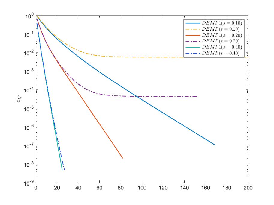
((a))

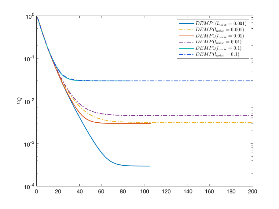
((b))

Figure 1: The impact of penalty parameter selection and the added termination condition on solving the PGO problem using the dominant eigenvalue method

As depicted in Figure 1, with noiseless data, DEMP1 converges roughly linearly. As the observation rate declines, the accuracy of DEMP diminishes markedly, whereas DEMP1 retains a linear error reduction. In noisy data scenarios, DEMP1 incurs lower errors. Incorporating the termination condition, DEMP1 halts iterations promptly when function value changes minimally, as evidenced by Figure 1. This validates our penalty parameter selection and termination condition, accelerating the algorithm while enhancing accuracy.

Therefore, when considering improvements to the dominant eigenvalue method based on the dual complex adjoint matrix in subsequent work, we directly compare with algorithm DEMP1.

Table 2: Numerical results on the impact of the penalty parameter selection and the added termination condition on solving the PGO problem using the dominant eigenvalue method under different noise levels and observation rates

algorithm		DEMP			DEMP1
$l_{\text{noise}}$	$s$	$e_{Q}$	$n_{iter}$	$time(s)$	$e_{Q}$	$n_{iter}$	$time(s)$
0	10$\%$	5.64e-3	200	1.63	1.04e-7	169	1.44
0	20$\%$	4.30e-5	153	1.05	2.02e-8	82	6.04e-1
0	40$\%$	4.88e-9	27	2.15e-1	4.66e-9	25	1.99e-1
0.1	10$\%$	2.96e-2	200	1.70	2.95e-2	87	9.36e-1
0.01	10$\%$	4.51e-3	200	1.58	2.95e-3	106	1.20
0.001	10$\%$	3.12e-3	200	2.50	2.95e-4	105	1.95

4.3.2 Improvements of the dominant eigenvalue algorithm based on the dual complex adjoint matrix under different noise levels

In this subsection, we present the numerical results of solving the PGO problem using algorithms DEMP1, DBDEMP, and DBDEMP1, respectively, under different noise levels, with a given observation rate $s=0.40$ and dimension $n=10$ in Table 3, and with a given observation rate $s=0.20$ and dimension $n=100$ in Table 4. All algorithms, DEMP1, DBDEMP, and DBDEMP1, use the parameters $k_{max}=200$, $\rho^{(0)}=0.01$, $\rho_{1}=1$, $d=2$, $\beta=10^{-6}$.

Table 3: The numerical results of solving the PGO problem using algorithms DEMP1, DBDEMP, and DBDEMP1 under different noise levels for given observation rate $s=0.40$ and dimension $n=10$

algorithm	$l_{\text{noise}}$	$e_{Q}$	$n_{iter}$	$time(s)$	$l_{\text{noise}}$	$e_{Q}$	$n_{iter}$	$time(s)$
DEMP1	0.1	4.28e-2	43.89	6.59e-1	0.01	4.23e-3	40.19	5.11e-1
	0.001	4.29e-4	40.03	5.02e-1	0	1.50e-7	54.84	6.73e-1
DBDEMP	0.1	3.95e-2	37.72	8.77e-3	0.01	3.91e-3	34.97	7.64e-3
	0.001	3.88e-4	35.53	6.35e-3	0	7.65e-8	46.24	8.77e-3
DBDEMP1	0.1	3.72e-2	37.20	8.26e-3	0.01	3.69e-3	33.91	6.59e-3
	0.001	3.66e-4	35.49	6.24e-3	0	1.01e-7	48.14	9.20e-3

It is worth noting that DEMP1 is not always valid in solving PGO problems. If the error $e_{Q}$ surpasses the noise level $l_{\text{noise}}$, particularly $e_{Q}>10^{-5}$ in noiseless cases, the solution is deemed ineffective. In our 100-trial experiments, DEMP1 faltered under varying noise levels ($l_{\text{noise}}=0.1,0.01,0.001,0$) for $s=0.40$ and $n=10$, failing 1, 4, 5, and 4 times respectively. In contrast, DBDEMP and DBDEMP1 consistently succeeded. At $s=0.20$ and $n=100$, all algorithms (DEMP1, DBDEMP, DBDEMP1) solved the problem effectively. This showcases the superiority of dual complex adjoint matrix based algorithms in terms of success rate for PGO problem.

Table 4: The numerical results of solving the PGO problem using algorithms DEMP1, DBDEMP, and DBDEMP1 under different noise levels for given $s=0.20$ and $n=100$

algorithm	$l_{\text{noise}}$	$e_{Q}$	$n_{iter}$	$time(s)$	$l_{\text{noise}}$	$e_{Q}$	$n_{iter}$	$time(s)$
DEMP1	0.1	2.08e-2	44.25	5.60e-1	0.01	2.10e-3	45.46	5.60e-1
	0.001	2.11e-4	47.14	6.94e-1	0	1.35e-8	66.33	8.32e-1
DBDEMP	0.1	1.96e-2	41.87	1.30e-1	0.01	1.99e-3	42.46	1.40e-1
	0.001	2.00e-4	44.39	1.60e-1	0	1.30e-8	64.18	2.09e-1
DBDEMP1	0.1	1.78e-2	41.25	1.26e-1	0.01	1.81e-3	41.50	1.22e-1
	0.001	1.82e-4	44.02	1.47e-1	0	1.38e-8	64.67	1.95e-1

As evident from Tables 3 and 4, DBDEMP and DBDEMP1 outperform DEMP1 in error $e_{Q}$. In noisy conditions, the error obtained by DBDEMP is reduced by $5\%$ compared to DEMP1, while the error obtained by DBDEMP1 is reduced by $12.5\%$ compared to DEMP1. For dmension $n=10$, DBDEMP and DBDEMP1 consume merely $1.5\%$ of the computation time of DEMP1, while for $n=100$, it is $25\%$. This underscores the role of dual complex adjoint matrix in enhancing accuracy and efficiency of solving PGO problem. In noisy conditions, DBDEMP1 outperforms DBDEMP slightly in terms of CPU time and the error $e_{Q}$, suggesting the benefits of utilizing the $F^{*}$-norm in solving the subproblem of PGO.

4.4 Improvements to the dominate eigenvalue algorithm based on the dual complex adjoint matrix under different observation rates

In this subsection, we present the numerical results of solving the PGO problem using algorithms DEMP1, DBDEMP, and DBDEMP1 at different observation rates with a given dimension $n=10$ or $n=100$ and noise level $l_{\text{noise}}=0.01$, which are shown in Table 5 and Table 6. All algorithms, DEMP1, DBDEMP, and DBDEMP1, use the parameters $k_{max}=200$, $\rho^{(0)}=0.01$, $\rho_{1}=1$, $d=2$, and $\beta=10^{-6}$.

In our 100-trial experiments, DEMP1 failed 13, 1, 1, 2 times for $n=10$ at $s=30\%,40\%,50\%,60\%$ respectively, and 34, 20, 0, 0 times for $n=100$ at $s=5\%,7.5\%,10\%,20\%$. Conversely, DBDEMP and DBDEMP1 consistently succeeded. As the observation rate $s$ decreased, the failure rate of DEMP1 increased, whereas both DBDEMP and DBDEMP1 maintained their effectiveness. This underscores the advantage of incorporating the dual complex adjoint matrix into solving PGO problem under low observation rates.

Table 5: The numerical results of solving the PGO problem using algorithms DEMP1, DBDEMP, and DBDEMP1 at different observation rates for given $n=10$ and $l_{\text{noise}}=0.01$

algorithm	$s$	$e_{Q}$	$n_{iter}$	$time(s)$	$s$	$e_{Q}$	$n_{iter}$	$time(s)$
DEMP1	30$\%$	5.08e-3	57.91	8.86e-1	40$\%$	4.26e-3	42.22	5.72e-1
	50$\%$	3.83e-3	29.44	3.02e-1	60$\%$	3.40e-3	22.48	2.68e-1
DBDEMP	30$\%$	4.62e-3	60.74	1.29e-2	40$\%$	3.93e-3	37.01	1.17e-2
	50$\%$	3.52e-3	24.27	4.69e-3	60$\%$	3.12e-3	17.22	4.07e-3
DBDEMP1	30$\%$	4.37e-3	58.55	1.15e-2	40$\%$	3.70e-3	35.76	1.04e-2
	50$\%$	3.32e-3	23.08	5.06e-3	60$\%$	2.95e-3	17.24	3.76e-3

Tables 5 and 6 reveal that DBDEMP and DBDEMP1 outperform DEMP1 in $e_{Q}$ errors. The error obtained by DBDEMP is reduced by $7.5\%$ compared to DEMP1, while the error obtained by DBDEMP1 is reduced by $13\%$ compared to DEMP1. For dimension $n=10$, DBDEMP and DBDEMP1 consume merely $2\%$ of the computation time of DEMP1, while for $n=100$, it is $25\%$. This underscores the role of dual complex adjoint matrix in enhancing accuracy and efficiency of solving PGO problem. In noisy conditions, DBDEMP1 outperforms DBDEMP slightly in terms of CPU time and the error $e_{Q}$, suggesting the benefits of utilizing the $F^{*}$-norm in solving the subproblem of PGO.

Table 6: The numerical results of solving the PGO problem using algorithms DEMP1, DBDEMP, and DBDEMP1 at different observation rates for given $n=100$ and $l_{\text{noise}}=0.01$

algorithm	$s$	$e_{Q}$	$n_{iter}$	$time(s)$	$s$	$e_{Q}$	$n_{iter}$	$time(s)$
DEMP1	5$\%$	4.16e-3	205.71	4.47	7.5$\%$	3.30e-3	129.66	3.07
	10$\%$	2.83e-3	106.32	1.53	20$\%$	2.08e-3	45.65	6.33e-1
DBDEMP	5$\%$	3.85e-3	370.47	9.84e-1	7.5$\%$	3.10e-3	176.20	4.84e-1
	10$\%$	2.66e-3	109.43	3.03e-1	20$\%$	1.96e-3	42.17	1.33e-1
DBDEMP1	5$\%$	3.54e-3	369.27	9.54e-1	7.5$\%$	2.84e-3	179.70	4.71e-1
	10$\%$	2.43e-3	106.47	2.84e-1	20$\%$	1.79e-3	41.39	1.26e-1

Through numerical experiments, we have confirmed that the new choice of penalty parameter and additional termination criteria enhances the accuracy and efficiency of the dominate eigenvalue algorithm for PGO problems. Furthermore, algorithms leveraging the dual complex adjoint matrix demonstrate superior accuracy, faster computation, and higher success rates, especially at low observation rates. Notably, employing the $F^{*}$-norm in solving subproblem of PGO further boosts accuracy and efficiency to a certian extent.

5 Final Remarks

In this paper, we delve into the eigenvalue problem and the matrix rank-k approximation problem of dual quaternion matrices by leveraging dual complex adjoint matrices. We transform the eigenvalue problem of dual quaternion matrices into that of dual complex adjoint matrices, leveraging this transformation to refine the power method, thereby achieving a higher numerical computation efficiency. Furthermore, based on the eigendecomposition of the dual complex adjoint matrix, we propose an algorithm (Algorithm 3) for computing all eigenvalues of dual quaternion matrices. This algorithm significantly outpaces the power method in terms of computation speed and mitigates the limitation of the power method, which may fail to solve some eigenvalues in certain cases. Addressing the pose graph optimization problem, we enhance the dominant eigenvalue algorithm by incorporating the power method based on the dual complex adjoint matrix and the rank-k approximation of dual quaternion Hermitian matrices. This enhancement leads to improvements in both accuracy and computation speed. This underscores the substantial applications of dual complex adjoint matrices within the domain of dual quaternion matrix theory. We anticipate that our research will serve as a foundation for future endeavors in this promising field.

References

• [1] Bultmann S, Li K, Hanebeck U D. Stereo visual SLAM based on unscented dual quaternion filtering[C]//2019 22th International Conference on Information Fusion (FUSION). IEEE, 2019: 1-8.
• [2] Bryson M, Sukkarieh S. Building a Robust Implementation of Bearing‐only Inertial SLAM for a UAV[J]. Journal of Field Robotics, 2007, 24(1‐2): 113-143.
• [3] Cadena C, Carlone L, Carrillo H, et al. Past, present, and future of simultaneous localization and mapping: Toward the robust-perception age[J]. IEEE Transactions on robotics, 2016, 32(6): 1309-1332.
• [4] Cheng J, Kim J, Jiang Z, et al. Dual quaternion-based graphical SLAM[J]. Robotics and Autonomous Systems, 2016, 77: 15-24.
• [5] Cui C, Qi L. A power method for computing the dominant eigenvalue of a dual quaternion Hermitian matrix[J]. Journal of Scientific Computing, 2024, 100(1): 21.
• [6] Carlone L, Tron R, Daniilidis K, et al. Initialization techniques for 3D SLAM: A survey on rotation estimation and its use in pose graph optimization[C]//2015 IEEE international conference on robotics and automation (ICRA). IEEE, 2015: 4597-4604.
• [7] Chen Y, Zhang L. Dual Complex Adjoint Matrix: Applications in Dual Quaternion Research[J]. arXiv preprint arXiv:2407.12635, 2024.
• [8] Daniilidis K. Hand-eye calibration using dual quaternions[J]. The International Journal of Robotics Research, 1999, 18(3): 286-298.
• [9] Duan S Q, Wang Q W, Duan X F. On Rayleigh Quotient Iteration for Dual Quaternion Hermitian Eigenvalue Problem[J]. arXiv preprint arXiv:2310.20290, 2023.
• [10] Grisetti G, Kümmerle R, Stachniss C, et al. A tutorial on graph-based SLAM[J]. IEEE Intelligent Transportation Systems Magazine, 2010, 2(4): 31-43.
• [11] Ling C, He H, Qi L, et al. von Neumann type trace inequality for dual quaternion matrices[J]. arXiv preprint arXiv:2204.09214, 2022.
• [12] Ling C, Qi L, Yan H. Minimax principle for eigenvalues of dual quaternion Hermitian matrices and generalized inverses of dual quaternion matrices[J]. Numerical Functional Analysis and Optimization, 2023, 44(13): 1371-1394.
• [13] Qi L, Luo Z. Eigenvalues and singular values of dual quaternion matrices[J]. arXiv preprint arXiv:2111.12211, 2021.
• [14] Qi L, Ling C, Yan H. Dual quaternions and dual quaternion vectors[J]. Communications on Applied Mathematics and Computation, 2022, 4(4): 1494-1508.
• [15] Qi L, Wang X, Luo Z. Dual quaternion matrices in multi-agent formation control[J]. arXiv preprint arXiv:2204.01229, 2022.
• [16] Wang H, Cui C, Liu X. Dual r-rank decomposition and its applications[J]. Computational and Applied Mathematics, 2023, 42(8): 349.
• [17] Wei T, Ding W, Wei Y. Singular value decomposition of dual matrices and its application to traveling wave identification in the brain[J]. SIAM Journal on Matrix Analysis and Applications, 2024, 45(1): 634-660.
• [18] Wei E, Jin S, Zhang Q, et al. Autonomous navigation of Mars probe using X-ray pulsars: modeling and results[J]. Advances in Space Research, 2013, 51(5): 849-857.
• [19] Williams S B, Newman P, Dissanayake G, et al. Autonomous underwater simultaneous localisation and map building[C]//Proceedings 2000 ICRA. Millennium Conference. IEEE International Conference on Robotics and Automation. Symposia Proceedings (Cat. No. 00CH37065). IEEE, 2000, 2: 1793-1798.
• [20] Zhang, Fuzhen. ”Quaternions and matrices of quaternions.” Linear algebra and its applications 251 (1997): 21-57.