Om$#\mathrm{2}$

Stochastic density functional theory for ions in a polar solvent

Abstract

In recent years, the theoretical description of electrical noise and fluctuation-induced effects in electrolytes has gained a renewed interest, enabled by stochastic field theories like stochastic density functional theory (SDFT). Such models, however, treat solvents implicitly, ignoring their generally polar nature. In the present study, starting from microscopic principles, we derive a fully explicit SDFT theory that applies to ions in a polar solvent. These equations are solved to compute observables like dynamic charge structure factors and dielectric susceptibilities. We unveil the relative importance of the different contributions (solvent, ions, cross terms) to the dynamics of electrolytes, which are key to understand the couplings between ions and the fluctuations of their microscopic environment.

Introduction.— Predicting analytically the structure and dynamics of electrolytes from microscopic considerations is a crucial challenge in chemical physics, with significant applications across various fields, from electrochemistry to soft matter physics. Going beyond their well-established average properties, such as their activity coefficient or their conductivity [1, 2], recent experimental research has unveiled the prominent role played by fluctuations on their dynamics [3, 4, 5, 6]. From the theoretical point of view, particle-based simulations (molecular or Langevin dynamics) as well as analytical descriptions of the underlying stochastic dynamics have enabled the study of the dynamical response properties of electrolytes, for instance through frequency-dependent conductivity [7, 8] or fluctuation-induced effects [9, 10, 11, 12, 13, 14, 15]. In particular, stochastic density functional theory (SDFT), that stems from the works of Kawasaki [16] and Dean [17] on the coarse-graining of interacting Langevin processes, has become a key tool to study the properties of electrolytes (such as their conductivity [18, 19, 20, 21, 22, 23, 24, 25], ionic correlations [26, 27] or viscosity [28]) as well as the static structure of polar liquids [29].

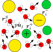
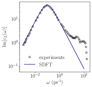
Figure 1: Left: System under study: $N_{I}$ anions and $N_{I}$ cations, at positions $\boldsymbol{r}_{i}^{\pm}$, are embedded in a solvent, made of $N_{S}$ molecules, described by their positions $\boldsymbol{r}_{j}^{S}$ and their orientations $\hat{\boldsymbol{u}}_{j}$. Right: Imaginary part of the longitudinal permittivity of pure water, computed theoretically from our SDFT approach, and compared to the experimental data reproduced from Ref. [30].

However, so far, SDFT has been limited to situations where the solvent in which the ions are embedded is described in an implicit way: this approach could therefore be seen as a stochastic extension of the classical Poisson-Nernst-Planck framework. Although it is able to capture some essential properties of electrolytes, it ignores the fact the solvent molecules also bear charge distribution, which can, to leading order, be represented by a polarization field, whose dynamics is coupled to the ionic charge density. Such couplings are key to understand the relationship between ions and their microscopic environment, which control numerous key processes, such as water autodissociation [31], dielectric solvation [32], or NMR relaxation of quadrupolar nuclei [33, 34]. The effect of the solvent on the ion dynamics has been studied from the numerical and theoretical point of view [35, 36, 37, 38], and it can be introduced in implicit solvent theories of the conductivity [7]. However, the mutual coupling of ion and solvent dynamics has received less attention. This aspect can be investigated using molecular simulations with an explicit solvent [39, 40, 41], but is much more challenging in analytical approaches.

The goal of this Letter is two-fold. First, we fill the theoretical gap that is set out in this introduction, and derive SDFT equations for ions in a polar solvent: starting from microscopic principles, our approach results in coupled stochastic equations obeyed by the ionic charge density and by the solvent polarization field. Second, these equations are solved to compute the correlation and response functions of the electrolytes, unveiling the relative importance of the different contributions (solvent, ions, cross terms) to the dynamics. As a perspective, given the strong interest raised by the use of SDFT to study charged systems at the level of fluctuations, we expect that the present work will bring insight in the fluctuation-induced effects that have been recently evidenced in electrolytes  [9, 10, 11, 12, 13, 14, 15].

Model.— We consider a binary electrolyte made of $N_{I}$ cations and $N_{I}$ anions of respective charge $\pm ze$. We denote by $\boldsymbol{r}_{i}^{\pm}(t)$ their positions. The electrolyte is embedded in a solvent represented by $N_{S}$ point charge dipoles, of dipolar moment $p$. We denote by $\boldsymbol{r}^{S}_{j}(t)$ their position and $\hat{\boldsymbol{u}}_{j}(t)$ their unit orientation vector (see Fig. 1). Even though some of the previous SDFT approaches accounted for hydrodynamic couplings [21, 22, 19, 11], the goal of the present study is to highlight the interplay between ionic current and solvent polarization dynamics. To this end, we will adopt a simple description, where both ions and solvent molecules obey overdamped Langevin dynamics. We denote by $\mu_{I}$ (resp. $\mu_{S}$) the bare mobility of the ions (resp. solvent molecules), and by $D_{I}=k_{\mathrm{B}}T\mu_{I}$ (resp. $D_{S}=k_{\mathrm{B}}T\mu_{S}$) the associated bare diffusion coefficients. We also denote by $D_{S}^{r}$ is the rotational diffusion coefficient of the solvent molecules, and $\mu_{S}^{r}$ the associated orientational mobility ($D_{S}^{r}=k_{\mathrm{B}}T\mu_{S}^{r}$). We introduce the stochastic density of cations and anions as $n_{\pm}(\boldsymbol{r},t)=\sum_{i=1}^{N_{I}}\delta(\boldsymbol{r}-\boldsymbol{r}_{i}^{\pm}(t))$, and that of solvent molecules, which has both translational and orientational degrees of freedom: $n_{S}(\boldsymbol{r},\hat{\boldsymbol{u}},t)=\sum_{j=1}^{N_{S}}\delta(\boldsymbol{r}-\boldsymbol{r}_{j}^{S}(t))\delta(\hat{\boldsymbol{u}}-\hat{\boldsymbol{u}}_{j}(t))$.

The electrostatic potential at a given point of the solution $\boldsymbol{r}$, denoted by $\varphi(\boldsymbol{r})$, is obtained by solving Poisson’s equation: $-\nabla^{2}\varphi(\boldsymbol{r})=[\rho_{I}(\boldsymbol{r})+\rho_{S}(\boldsymbol{r})]/\varepsilon_{0}$ , where $\rho_{I}=ze(n_{+}-n_{-})$ is the charge density of the ions and $\rho_{S}$ is the charge density associated to the solvent. Within the dipolar approximation (i.e. at distances much larger than the typical size of a solvent molecule), $\rho_{S}(\boldsymbol{r})\simeq-\nabla\cdot\boldsymbol{P}(\boldsymbol{r})$, where we define the polarization field of the solvent as $\boldsymbol{P}(\boldsymbol{r},t)=\int\mathrm{d}\hat{\boldsymbol{u}}\;p\hat{\boldsymbol{u}}n_{S}(\boldsymbol{r},\hat{\boldsymbol{u}},t)$. The solution to Poisson’s equation is then $\varphi(\boldsymbol{r},t)=\int\mathrm{d}\boldsymbol{r}^{\prime}\;\mathcal{G}(\boldsymbol{r}-\boldsymbol{r}^{\prime})[\rho_{I}(\boldsymbol{r}^{\prime},t)-\nabla\cdot\boldsymbol{P}(\boldsymbol{r}^{\prime},t)]$, with the Green function $\mathcal{G}(\boldsymbol{r})=1/(4\pi\varepsilon_{0}|\boldsymbol{r}|)$.

Stochastic density functional theory.— In the overdamped limit, the state of the system is fully characterized by the positions of the ions $\boldsymbol{r}_{i}^{\pm}$, and the position and orientations of the solvent molecules $\boldsymbol{r}_{j}^{S}$ and $\hat{\boldsymbol{u}}_{j}$. The evolution equations read:

$$\frac{\mathrm{d}\boldsymbol{r}_{i}^{\pm}}{\mathrm{d}t} =\mp\mu_{I}ze\nabla\varphi(\boldsymbol{r}_{i}^{\pm})+\sqrt{2D_{\pm}}\boldsymbol{\xi}_{i}^{\pm}(t),$$ (1)

$$\frac{\mathrm{d}\boldsymbol{r}^{S}_{j}}{\mathrm{d}t} =-\mu_{S}(p\hat{\boldsymbol{u}}_{j}\cdot\nabla)\nabla\varphi(\boldsymbol{r}_{j}^{S})+\sqrt{2D_{S}}\boldsymbol{\xi}_{j}^{S}(t),$$ (2)

$$\frac{\mathrm{d}\hat{\boldsymbol{u}}_{j}}{\mathrm{d}t} =\left\{-[\mu_{S}^{r}p\hat{\boldsymbol{u}}_{j}\times\nabla\varphi(\boldsymbol{r}_{j}^{S})]+\sqrt{2D_{S}^{r}}\boldsymbol{\xi}_{j}^{S,r}(t)\right\}\times\hat{\boldsymbol{u}}_{j},$$ (3)

where the noises $\boldsymbol{\xi}_{a}^{\alpha}(t)$ are uncorrelated Gaussian white noises of zero average and unit variance, i.e. $\langle\xi_{i,n}^{\alpha}(t)\xi_{j,m}^{\beta}(t^{\prime})\rangle=\delta_{\alpha\beta}\delta_{mn}\delta_{ij}\delta(t-t^{\prime})$, where $n$ or $m$ are components of the vectors. Note that we assumed here that the ions only interact through electrostatic interactions, and that short-range repulsive interactions are neglected.

Starting from Eqs. (1)-(3), the derivations of the equations satisfied by the ionic charge density $\rho_{I}=ze(n_{+}-n_{-})$ and the total number density $\mathcal{C}=n_{+}+n_{-}$ of ions are standard and rely on Itô’s lemma [17, 18]. One gets:

$$\partial_{t}\rho_{I} = D_{I}\nabla^{2}\rho_{I}+\mu_{I}(ze)^{2}\nabla\cdot(\mathcal{C}\nabla\varphi)$$ (4)

$$+\nabla\cdot(ze\sqrt{2D_{I}\mathcal{C}}\boldsymbol{\zeta}_{\rho_{I}}),$$

$$\partial_{t}\mathcal{C} = D_{I}\nabla^{2}\mathcal{C}+\mu_{I}\nabla\cdot(\rho_{I}\nabla\varphi)+\nabla\cdot(\sqrt{2D_{I}\mathcal{C}}\boldsymbol{\zeta}_{\mathcal{C}}),$$ (5)

where $\boldsymbol{\zeta}_{\alpha}(\boldsymbol{r},t)$ are uncorrelated Gaussian white noises of zero average and unit variance (and similarly in the next equation). In contrast, the derivation of the equation satisfied by $n_{S}$ is more subtle as it involves two variables, one of them being an orientational degree of freedom, see Supplementary Material (SM) [43]. It reads:

$$\partial_{t}n_{S}(\boldsymbol{r},\hat{\boldsymbol{u}},t)=D_{S}\nabla^{2}_{\boldsymbol{r}}n_{S}+D_{S}^{r}\boldsymbol{\mathcal{R}}_{\hat{\boldsymbol{u}}}^{2}n_{S}$$ (6)

$$+\nabla_{\boldsymbol{r}}\cdot[n_{S}\mu_{S}p(\hat{\boldsymbol{u}}\cdot\nabla)\nabla\varphi(\boldsymbol{r})]+\boldsymbol{\mathcal{R}}_{\hat{\boldsymbol{u}}}\cdot[n_{S}\mu_{S}^{r}p\hat{\boldsymbol{u}}\times\nabla\varphi(\boldsymbol{r})]$$

$$+\nabla_{\boldsymbol{r}}\cdot(\sqrt{2D_{S}n_{S}}\boldsymbol{\zeta}_{S}(\boldsymbol{r},t))+\boldsymbol{\mathcal{R}}_{\hat{\boldsymbol{u}}}\cdot(\sqrt{2D_{S}^{r}n_{S}}\boldsymbol{\zeta}_{S,r}(\boldsymbol{r},t))$$

where $\boldsymbol{\mathcal{R}}_{\hat{\boldsymbol{u}}}=\hat{\boldsymbol{u}}\times\nabla_{\hat{\boldsymbol{u}}}$ is the rotational gradient operator [44]. Finally, note that, within the dipolar approximation, Eqs. (4)-(6) form a closed set of equations for $\rho_{I}$, $\mathcal{C}$ and $n_{S}$, since the electrostatic potential $\varphi$ is related to $\rho_{I}$ and $\rho_{S}$ through $\varphi(\boldsymbol{r},t)=\int\mathrm{d}\boldsymbol{r}^{\prime}\;\mathcal{G}(\boldsymbol{r}-\boldsymbol{r}^{\prime})[\rho_{I}(\boldsymbol{r}^{\prime},t)+\rho_{S}(\boldsymbol{r}^{\prime},t)]$.

Although Eqs. (4)-(6) are exact reformulations of the microscopic overdamped Langevin dynamics, they are rather unpractical, since they are nonlinear. To make analytical progress, we linearize them around a uniform, time-independent state [10, 45]. More precisely, denoting by $C_{I}$ the concentration of the electrolyte, we write $n_{\pm}=C_{I}+\delta n_{\pm}$, which implies $\rho_{I}=ze(\delta n_{+}-\delta n_{-})$. At linear order in the perturbation, the equation for $\rho_{I}$ is decoupled from that on $c$:

$$\partial_{t}\rho_{I}(\boldsymbol{r},t)=D\nabla^{2}\rho_{I}+2\mu(ze)^{2}C_{I}\nabla^{2}\varphi+ze\sqrt{4DC_{I}}{\eta}_{\rho_{I}}.$$ (7)

Similarly, the density of the solvent is expanded as $n_{S}={C_{S}}/{4\pi}+c_{S}$, where $C_{S}$ is the concentration of solvent molecules, and the $1/4\pi$ factor accounts for the uniform density of orientations. The equation satisfied by the polarisation is deduced using $\boldsymbol{P}(\boldsymbol{r},t)=\int\mathrm{d}\hat{\boldsymbol{u}}\;p\hat{\boldsymbol{u}}c_{S}(\boldsymbol{r},\hat{\boldsymbol{u}},t)$:

$$\partial_{t}\boldsymbol{P}(\boldsymbol{r},t)=D_{S}\nabla^{2}\boldsymbol{P}-2D_{S}^{r}\boldsymbol{P}$$

$$+\frac{1}{3}p^{2}C_{S}\nabla(\mu_{S}\nabla^{2}\varphi-2\mu_{S}^{r}\varphi)+\boldsymbol{\Xi}(\boldsymbol{r},t),$$ (8)

with $\langle\Xi_{k}(\boldsymbol{r},t)\Xi_{l}(\boldsymbol{r}^{\prime},t^{\prime})\rangle=\frac{2p^{2}C_{S}}{3}\delta_{kl}\delta(t-t^{\prime})(-D_{S}\nabla^{2}+2D_{S}^{R})\delta(\boldsymbol{r}-\boldsymbol{r}^{\prime})$. Note that, for a system without ions, the deterministic term in rhs of Eq. (8) can be rewritten under the form $-\frac{\delta}{\delta\boldsymbol{P}}\mathcal{F}[\boldsymbol{P}]$, where the free energy functional $\mathcal{F}[\boldsymbol{P}]$ is here derived from microscopic considerations [43], and may be compared to previously proposed expressions based on symmetry considerations [46, 47, 48, 49, 50, 51].

Evolution equations for the charge densities.— Finally, the evolution equation for $\rho_{S}$ is deduced by taking the divergence of Eq. (8). In Fourier space , we find the following coupled stochastic equations for the ion and solvent charge densities:

$$\partial_{t}\begin{pmatrix}\tilde{\rho}_{I}(\boldsymbol{q},t)\\ \tilde{\rho}_{S}(\boldsymbol{q},t)\end{pmatrix}=-\mathbf{M}\begin{pmatrix}\tilde{\rho}_{I}(\boldsymbol{q},t)\\ \tilde{\rho}_{S}(\boldsymbol{q},t)\end{pmatrix}+\begin{pmatrix}\Xi_{I}(\boldsymbol{q},t)\\ \Xi_{S}(\boldsymbol{q},t)\end{pmatrix},$$ (9)

with

$$\mathbf{M}=\begin{pmatrix}D_{I}(q^{2}+\kappa_{I}^{2})&D_{I}\kappa_{I}^{2}\\ D_{S}\kappa_{S}(q)^{2}&D_{S}(q^{2}+\kappa_{S}(q)^{2})+2D_{S}^{r}\end{pmatrix},$$ (10)

where we introduced the Debye screening length of the electrolyte $\kappa_{I}^{-1}$, which is such that $\kappa_{I}^{2}=\frac{2C_{I}(ze)^{2}}{\varepsilon_{0}k_{\mathrm{B}}T}$, and the wavenumber-dependent screening length associated with the charge polarization of the solvent $\kappa_{S}(q)^{2}=\frac{2p^{2}C_{S}}{3\varepsilon_{0}k_{\mathrm{B}}Ta^{2}}\left(1+\frac{q^{2}a^{2}}{2}\right)$, where we introduced $a\equiv(D_{S}/D_{S}^{r})^{1/2}$, which is the typical size of a solvent molecule. The noises $\Xi_{I}$ and $\Xi_{S}$ have zero average and correlations $\langle\Xi_{\alpha}(\boldsymbol{q},t)\Xi_{\beta}(\boldsymbol{q}^{\prime},t^{\prime})\rangle=2q^{2}\varepsilon_{0}k_{\mathrm{B}}TD_{\alpha}\kappa_{\alpha}^{2}(2\pi)^{d}\delta(\boldsymbol{q}+\boldsymbol{q}^{\prime})\delta(t-t^{\prime})\delta_{\alpha\beta}$. Eq. (9) is formally solved as $\tilde{\rho}_{\alpha}(\boldsymbol{q},t)=\int_{-\infty}^{t}\mathrm{d}t^{\prime}\;\mathcal{M}_{\alpha\beta}(t-t^{\prime})\Xi_{\beta}(\boldsymbol{q},t^{\prime})$, where $\boldsymbol{\mathcal{M}}(t)=\exp(-t\mathbf{M})$, and where repeated indices are implicitly summed upon.

Eq. (9) is the central result of this Letter, and several comments are in order: (i) The coupled equations for the fields $\tilde{\rho}_{I}$ and $\tilde{\rho}_{S}$ are fully explicit and actually depend on a reduced set of parameters: the self-diffusion coefficients of ions and solvent molecules $D_{I}$ and $D_{S}$, as well as their respective screening lengths $\kappa_{I}$ and $\kappa_{S}(q)$, which are themselves known in terms of the microscopic parameters of the model; (ii) These equations give access to the coupled statistics of the ionic charge density $\rho_{I}$ and to the charge polarization $\rho_{S}$, as well as to many derived quantities of experimental interest, that will be described in what follows; (iii) It is straighforward to show that the eigenvalues of $\mathbf{M}$ are always positive, in such a way that the solutions to Eq. (9) never diverge (which is a consequence of the mutual relaxation of ionic currents and solvent polarization); (iv) As a consequence of the linearization procedure, the stochastic fields $\tilde{\rho}_{I}$ and $\tilde{\rho}_{S}$ have Gaussian statistics.

Static and dynamic charge structure factors.— From the solution to the matrix equation obeyed by the charge density fields $\tilde{\rho}_{I}$ and $\tilde{\rho}_{S}$, we deduce the charge dynamic structure factors (or intermediate scattering functions), which are defined as $F_{\alpha\beta}(q,t)=(\mathcal{N}_{\alpha}\mathcal{N}_{\beta})^{-1/2}\langle\tilde{\rho}_{\alpha}(\boldsymbol{q},t)\tilde{\rho}_{\beta}(-\boldsymbol{q},0)\rangle$ [53], where we write $\mathcal{N}_{I}=2N_{I}$ and $\mathcal{N}_{S}=N_{S}$ for simplicity (we also write $C^{\text{tot}}_{I}=2C_{I}$ and $C^{\text{tot}}_{S}=C_{S}$). Note that this definition actually holds for a finite system in a volume $V$: our results, which were implicitly derived in the thermodynamic limit, can be mapped onto finite systems, which are of interest in molecular dynamics simulations for instance, by making the change $(2\pi)^{d}\delta(\boldsymbol{q}+\boldsymbol{q}^{\prime})\to V\delta_{\boldsymbol{q},-\boldsymbol{q}^{\prime}}$. We find:

$$F_{\alpha\beta}(q,t)=\frac{2q^{2}\varepsilon_{0}k_{\mathrm{B}}T}{(C^{\text{tot}}_{\alpha}C^{\text{tot}}_{\beta})^{1/2}}\sum_{\begin{subarray}{c}\gamma\in\{S,I\}\\ \nu=\pm 1\end{subarray}}D_{\gamma}\kappa_{\gamma}^{2}C_{\alpha\gamma,\beta\gamma}^{(\nu)}\mathrm{e}^{-\lambda_{\nu}|t|},$$ (11)

where the coefficients of the fourth-rank tensors $\mathbf{C}^{(\nu)}$ can be expressed simply in terms of the eigenvalues $\lambda_{\nu}$ and entries of $\mathbf{M}$ [43]. From this expression, we also define the static charge structure factors $\mathcal{S}_{\alpha\beta}(q)=F_{\alpha\beta}(q,0)$ as well as the dynamic charge structure factors in frequency space: $\tilde{F}_{\alpha\beta}(q,\omega)\equiv\int\mathrm{d}t\;\mathrm{e}^{-\mathrm{i}\omega t}F_{\alpha\beta}(q,t)$.

The total structure factor is $F_{\text{tot}}(q,t)=\sum_{\alpha,\beta\in\{I,S\}}\frac{(C^{\text{tot}}_{\alpha}C^{\text{tot}}_{\beta})^{1/2}}{C^{\text{tot}}_{I}+C^{\text{tot}}_{S}}F_{\alpha\beta}(q,t)$. We can verify that our model fulfils the electroneutrality condition, as $\lim_{q\rightarrow 0}F_{\text{tot}}(q,t)=0$ for any $t$. In particular, the static total structure factor follows the second moment Stillinger-Lovett condition, $\mathcal{S}_{\text{tot}}(q)=F_{\text{tot}}(q,0)\sim\varepsilon_{0}k_{\mathrm{B}}Tq^{2}$, which reflects the fact that our system is a perfect conductor [54]. In addition, in the static limit, we get the ion-ion charge structure factor $\mathcal{S}_{II}(q)\sim_{q\to 0}(ze)^{2}q^{2}\varepsilon_{\text{w}}/\kappa_{I}^{2}$, with $\varepsilon_{\text{w}}$ the permittivity of pure solvent in this model, which will be discussed below. This expression coincides with the one that is obtained by considering ions in an implicit solvent of permittivity $\varepsilon_{\text{w}}$, where $F_{\text{imp}}(q,t)=\frac{(ze)^{2}q^{2}}{q^{2}+\kappa_{\text{imp}}^{2}}\mathrm{e}^{-D_{I}(q^{2}+\kappa_{\text{imp}}^{2})t}$ [43] (with $\kappa_{\mathrm{imp}}^{2}=\frac{2C_{I}(ze)^{2}}{\varepsilon_{\text{w}}\varepsilon_{0}k_{\mathrm{B}}T}$), from which we deduce $\mathcal{S}^{\text{imp}}_{II}(q)\sim_{q\to 0}(ze)^{2}q^{2}/\kappa_{\text{imp}}^{2}$.

Finally, to characterize the dynamics of the ions, we define the ionic relaxation time as $\tau_{II}(q)=\tilde{F}_{II}(q,\omega=0)/2F_{II}(q,t=0)$. In the zero-$q$ limit, the ionic relaxation time of the implicit model is the Debye time, $\tau_{II}^{\text{imp}}(q=0)=\frac{1}{D_{I}\kappa_{\text{imp}}^{2}}$, while our models gives $\tau_{II}(q=0)=\frac{1}{D_{I}\kappa_{\text{imp}}^{2}}+\frac{\varepsilon_{\text{w}}-1}{2\varepsilon_{\text{w}}D_{S}^{r}}$. This shows that explicit solvent molecules tend to increase the ionic relaxation time. Note that the Debye model is retrieved when $D_{S}^{r}\ll(\varepsilon_{\text{w}}-1)D_{I}\kappa_{\text{imp}}^{2}/2\varepsilon_{\text{w}}$, i.e. in the limit where solvent molecules relax much faster than ions.

Dieletric susceptibility.— Within linear response, if the electrolyte is submitted to a small external field $\boldsymbol{E}_{0}$, the polarisation of the electrolyte reads, in Fourier space: $\boldsymbol{P}(\boldsymbol{q},\omega)=\boldsymbol{\chi}_{\boldsymbol{P}}(\boldsymbol{q},\omega)\cdot\boldsymbol{E}_{0}(\boldsymbol{q},\omega)$, and the ionic current, defined as $\boldsymbol{j}(\boldsymbol{r},t)=\sum_{\nu=\pm 1}\sum_{i}(\nu ze)\boldsymbol{v}_{i}^{\nu}(t)\delta(\boldsymbol{r}-\boldsymbol{r}_{i}^{\nu}(t))$ (where $\boldsymbol{v}_{i}^{\nu}$ is the velocity of the $i$-th ion of species $\nu$), is related to the external field through $\boldsymbol{j}(\boldsymbol{q},\omega)=\boldsymbol{\chi}_{\boldsymbol{j}}(\boldsymbol{q},\omega)\cdot\boldsymbol{E}_{0}(\boldsymbol{q},\omega)$, where $\boldsymbol{\chi}_{\boldsymbol{P}}$ and $\boldsymbol{\chi}_{\boldsymbol{j}}$ are susceptibility tensors, characterizing the response of the solvent and of the ions, respectively. The total susceptibility is $\boldsymbol{\chi}=\boldsymbol{\chi}_{\boldsymbol{P}}+\frac{\mathrm{i}}{\omega\varepsilon_{0}}\boldsymbol{\chi}_{\boldsymbol{j}}$ [55]. Computing the susceptibility tensor from microscopic and stochastic quantities is a subtle task, that has been discussed by many authors, both in the case of pure dipolar solvent [56, 30, 57], and in the case of an electrolyte [58, 59, 60]. Here, we will only be interested in the $|\boldsymbol{q}|\to 0$ limit of the susceptibility tensor, in which one gets [58]: $\boldsymbol{\chi}_{\boldsymbol{P}}(\omega)=(\varepsilon_{0}k_{\mathrm{B}}TV)^{-1}[\langle\boldsymbol{P}\boldsymbol{P}\rangle(0)+\int_{0}^{\infty}\mathrm{d}t\;\mathrm{e}^{\mathrm{i}\omega t}(\mathrm{i}\omega\langle\boldsymbol{P}\boldsymbol{P}\rangle(t)+\langle\boldsymbol{P}\boldsymbol{j}\rangle(t))]$ and $\boldsymbol{\chi}_{\boldsymbol{j}}(\omega)=(k_{\mathrm{B}}TV)^{-1}\int_{0}^{\infty}\mathrm{d}t\;\mathrm{e}^{\mathrm{i}\omega t}(\langle\boldsymbol{j}\boldsymbol{j}\rangle(t)+\mathrm{i}\omega\langle\boldsymbol{P}\boldsymbol{j}\rangle(t))$ where we used the shorthand notation $\langle\boldsymbol{A}\boldsymbol{B}\rangle(t)=\lim_{\boldsymbol{q}\to 0\\ }\langle\boldsymbol{A}(\boldsymbol{q},t)\cdot\boldsymbol{B}(-\boldsymbol{q},0)\rangle$. Importantly, all the correlation functions that appear in these relations can be computed directly from our SDFT approach [43].

Calibration of the model.— To calibrate the three independent parameters that describe our explicit solvent ($\kappa_{S}(0)$, $D_{S}^{r}$ and $a$), we compute the longitudinal permittivity of pure water, i.e. in the limit $C_{I}\to 0$ of our model. It is related to the susceptibility defined above through $\varepsilon_{L}(\omega)=1/[1-\chi_{L}(\omega)]$ [53], where $\chi_{L}$ is the longitudinal part of the susceptibility tensor . We get $\varepsilon_{L}(\omega)=\varepsilon_{0}+\frac{\varepsilon_{\text{w}}-\varepsilon_{0}}{1-\mathrm{i}\omega\tau_{S}}$, with $\tau_{S}=1/2D_{S}^{r}$ and $\varepsilon_{\text{w}}=1+\frac{p^{2}C_{S}}{3\varepsilon_{0}k_{\mathrm{B}}T}$. Importantly, this provides an estimate of the relative permittivity involved in the implicit description from microscopic considerations, and corresponds to the expression for a gas of interacting dipoles in the mean-field limit [62]. Comparison with experimental data [Fig. 1, right] yields $\varepsilon_{\text{w}}\simeq 78.5\varepsilon_{0}$ and $\tau\simeq 10$ ps, which enforces $\kappa_{S}(0)\simeq 12.4/a$ and $D_{S}^{r}\simeq 0.05$ ps^-1. The value of $a$ is chosen in such a way that the (self) translational diffusion coefficient of water molecules $D_{S}=a^{2}D_{S}^{r}$ matches the values typically measured at 25°C ($2.3\text{\times}{10}^{-9}$ m^2.s^-1): this imposes $a\simeq 2.14$ Å. Consequently, given the expression of $\kappa_{S}(0)$, the product $p^{2}C_{S}$ is also fixed: if one imposes $C_{S}\simeq 55$ M (the typical molar concentration of water under normal conditions), then one finds $p=$1.4$~{}\unit{D}$, which is reasonably close the value of the dipolar moment of a water molecule ($\simeq$1.8$~{}\unit{D}$ in gas phase or $\simeq$2.6$~{}\unit{D}$ in liquid phase [63]).

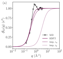
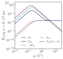
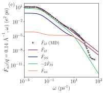
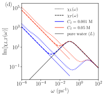
Figure 2: (a) Static charge structure factor of the ions only, as a function of the wavevector $q$. Results from our SDFT approach are compared and with the implicit solvent model with permittivity $\varepsilon_{\text{w}}$ (resp. $\varepsilon_{0}$), i.e. with Debye length $\kappa_{\text{imp}}$ (resp. $\kappa_{I}$). (b) Zero-frequency dynamic charge structure factors, where the different contributions are split. For comparison, the result for pure water ($C_{I}=0$) is shown. (c) Frequency dependence of the dynamic charge structure factors for $q=0.14$ Å^-1. (a-c) In these plots, we consider a 1:1 electrolyte of concentration $C_{I}=1.2$ M. (a,c) Symbols: results from molecular dynamics simulations reproduced from Ref. [41]. (d) Imaginary part of the transverse and longitudinal components of the total susceptibility tensor $\boldsymbol{\chi}(\omega)$. Dashed lines: $\sigma_{0}/\varepsilon_{0}\omega$. See SM [43] for other numerical parameters.

Numerical estimates.— Using these numerical parameters, we first compute the static structure factor of the ions $\mathcal{S}_{II}(q)$, and plot it on Fig. 2(a). We find that the expression computed within our explicit solvent model is very close to the expression that can be computed with the implicit model approach, i.e. with the Debye screening length $\kappa_{\text{imp}}$: this validates the model beyond the $q=0$ limit that was employed for calibration. We also study the $q$-dependence of the dynamic charge structure factors [Fig. 2(b)] and split the different contributions (ions, solvent, cross terms). Importantly, and just like in molecular dynamics simulations [41], we observe that the cross water-ion correlations, which are negative, are sufficiently strong to cancel the contributions from ions and solvent at small $q$. At large wavevectors, the total dynamic structure factor is equal to that of pure water, which tends to a constant, as expected in the present case where short-range interactions between molecules are ignored. For a fixed value of the wavevector ($q=0.14$ Å^-1, which corresponds to distances where short-range interactions do not play a significant role, and where our theory should be most valid), we plot the frequency-dependence of the dynamic structure factor and obtain a good agreement with results from MD simulations for the ionic contribution [Fig. 2(c)]: this validates our approach beyond the static limit. The analysis of the other contributions show that, at large frequencies, the cross contributions become subdominant, and do not contribute anymore to the total dynamic structure factor.

Finally, we turn to the dielectric response of the electrolyte. The imaginary parts of transverse and longitudinal components of the susceptibility tensor $\boldsymbol{\chi}(\omega)$ are shown on Fig. 2(d). The transverse components display crossovers at the characteristic frequencies $\sim D_{I}\kappa_{\text{imp}}^{2}$ and $\sim D_{S}^{r}$, which are respectively the Debye relaxation time of the ions and the typical persistence of the orientation of the water molecules. This is consistent with previous observations from molecular simulations [39, 40]. Finally, we retrieve that the small frequency limit of the imaginary part of the susceptibility diverges because of the overall conductivity of the system, which is non-zero in the presence of ions. Indeed, one gets $\text{Im}[{\chi}_{\alpha}(\omega)]\sim c_{\alpha}\sigma_{0}/\varepsilon_{0}\omega$, where $\sigma_{0}=\varepsilon_{0}D_{I}\kappa_{I}^{2}$ is the ideal conductivity of the ions in vacuum, and where $c_{\alpha}=2$ for $\alpha=L$ and $c_{\alpha}=1$ for $\alpha=T$.

Perspectives.— Several directions could be followed in order to refine the present theoretical framework: (i) the short-range interactions between the ions could be accounted for by combining SDFT with closure schemes such as the Mean Spherical Approximation [64, 65]. This could extend the relevance of our model beyond the small-$q$ limit, in particular to compare the $q$-dependence of the solvent permittivity with alternative approaches [66, 30]; (ii) hydrodynamic couplings between the ions and the solvent could be incorporated, in order to ensure momentum conservation within the solvent, as done previously at the SDFT level without taking into account the explicit polarization [21, 22, 19, 11].

Acknowledgments.— The authors thank Michiel Sprik, Steve Cox, Vincent Démery, Thê Hoang Ngoc Minh, Haim Diamant, and David Andelman for discussions on this topic, and Marie Jardat for comments on the manuscript. This project received funding from the European Research Council under the European Union’s Horizon 2020 research and innovation program (grant agreement no. 863473).

References

- Harned and Owen [1943] H. S. Harned and B. B. Owen, The Physical Chemistry of Electrolyte Solutions (American Chemical Society Monograph Series, 1943).
- Robinson and Stokes [2002] R. A. Robinson and R. H. Stokes, Electrolyte Solutions (Dover Publications, 2002).
- Heerema et al. [2015] S. J. Heerema, G. F. Schneider, M. Rozemuller, L. Vicarelli, H. W. Zandbergen, and C. Dekker, Nanotechnology 26, 074001 (2015).
- Vasilescu et al. [1974] D. Vasilescu, M. Teboul, H. Kranck, and F. Gutmann, Electrochimica Acta 19, 181 (1974).
- Mathwig et al. [2012] K. Mathwig, D. Mampallil, S. Kang, and S. G. Lemay, Phys. Rev. Lett. 109, 118302 (2012).
- Secchi et al. [2016] E. Secchi, A. Niguès, L. Jubin, A. Siria, and L. Bocquet, Phys. Rev. Lett. 116, 154501 (2016).
- Chandra and Bagchi [2000] A. Chandra and B. Bagchi, J. Chem. Phys. 112, 1876 (2000).
- Yamaguchi et al. [2007] T. Yamaguchi, T. Matsuoka, and S. Koda, J. Chem. Phys. 127, 234501 (2007).
- Lu et al. [2015] B. S. Lu, D. S. Dean, and R. Podgornik, Europhys. Lett. 112, 20001 (2015).
- Dean and Podgornik [2014] D. S. Dean and R. Podgornik, Phys. Rev. E 89, 032117 (2014).
- Péraud et al. [2017] J. P. Péraud, A. J. Nonaka, J. B. Bell, A. Donev, and A. L. Garcia, Proceedings of the National Academy of Sciences of the United States of America 114, 10829 (2017).
- Lee et al. [2018] A. A. Lee, J. P. Hansen, O. Bernard, and B. Rotenberg, Mol. Phys. 116, 3147 (2018).
- Mahdisoltani and Golestanian [2021a] S. Mahdisoltani and R. Golestanian, Phys. Rev. Lett. 126, 158002 (2021a).
- Mahdisoltani and Golestanian [2021b] S. Mahdisoltani and R. Golestanian, New Journal of Physics 23, 073034 (2021b).
- Du et al. [2024] G. Du, D. S. Dean, B. Miao, and R. Podgornik, (2024), arXiv:2404.06028 .
- Kawasaki [1994] K. Kawasaki, Physica A 208, 35 (1994).
- Dean [1996] D. S. Dean, J. Phys. A: Math. Gen. 29, L613 (1996).
- Démery and Dean [2015] V. Démery and D. S. Dean, J. Stat. Mech. 2016, 023106 (2015).
- Péraud et al. [2016] J.-P. Péraud, A. Nonaka, A. Chaudhri, J. B. Bell, A. Donev, and A. L. Garcia, Physical Review Fluids 1, 074103 (2016).
- Donev et al. [2019] A. Donev, A. L. Garcia, J. P. Péraud, A. J. Nonaka, and J. B. Bell, Current Opinion in Electrochemistry 13, 1 (2019).
- Avni et al. [2022a] Y. Avni, R. M. Adar, D. Andelman, and H. Orland, Phys. Rev. Lett. 128, 98002 (2022a).
- Avni et al. [2022b] Y. Avni, D. Andelman, and H. Orland, J. Chem. Phys. 157, 154502 (2022b).
- Bonneau et al. [2023] H. Bonneau, V. Démery, and E. Raphaël, J. Stat. Mech. 2023, 073205 (2023).
- Hoang Ngoc et al. [2023] M.-T. Hoang Ngoc, B. Rotenberg, and S. Marbach, Faraday Discussions 246, 225 (2023).
- Berthoumieux et al. [2024] H. Berthoumieux, V. Démery, and A. C. Maggs, (2024), arXiv:2405.05882 .
- Frusawa [2020] H. Frusawa, Entropy 22, 34 (2020).
- Frusawa [2022] H. Frusawa, Soft Matter 18, 4280 (2022).
- Robin [2024] P. Robin, J. Chem. Phys. 160, 064503 (2024).
- Déjardin et al. [2018] P. M. Déjardin, Y. Cornaton, P. Ghesquière, C. Caliot, and R. Brouzet, J. Chem. Phys. 148, 044504 (2018).
- Bopp et al. [1998] P. A. Bopp, A. A. Kornyshev, and G. Sutmann, J. Chem. Phys. 109, 1939 (1998).
- Geissler et al. [2001] P. L. Geissler, C. Dellago, D. Chandler, J. Hutter, and M. Parrinello, Science 291, 2121 (2001).
- Song et al. [1996] X. Song, D. Chandler, and R. A. Marcus, J. Phys. Chem. 100, 11954 (1996).
- Chubak et al. [2021] I. Chubak, L. Scalfi, A. Carof, and B. Rotenberg, J. Chem. Th. Comp. 17, 6006 (2021).
- Chubak et al. [2023] I. Chubak, L. Alon, E. V. Silletta, G. Madelin, A. Jerschow, and B. Rotenberg, Nature Communications 14, 84 (2023).
- Hubbard and Onsager [1977] J. Hubbard and L. Onsager, J. Chem. Phys. 67, 4850 (1977).
- Hubbard [1978] J. B. Hubbard, J. Chem. Phys. 68, 1649 (1978).
- Koneshan et al. [1998] S. Koneshan, J. C. Rasaiah, R. M. Lynden-Bell, and S. H. Lee, J. Phys. Chem. B 102, 4193 (1998).
- Banerjee and Bagchi [2019] P. Banerjee and B. Bagchi, J. Chem. Phys. 150 (2019).
- Sega et al. [2013] M. Sega, S. S. Kantorovich, A. Arnold, and C. Holm, in Recent Advances in Broadband Dielectric Spectroscopy, edited by Y. P. Kalmykov (Springer Netherlands, 2013) pp. 103–122.
- Sega et al. [2014] M. Sega, S. S. Kantorovich, C. Holm, and A. Arnold, J. Chem. Phys. 140 (2014).
- [41] M.-T. Hoang Ngoc, J. Kim, G. Pireddu, I. Chubak, S. Nair, and B. Rotenberg, Faraday Discussions 246, 198.
- Note [1] Note that we make the choice to use SI units throughout the paper: the mapping to cgs or Gaussian units, which are still used by many authors, is typically done through the change .
- [43] Supplemental Material .
- Doi and Edwards [1988] M. Doi and S. F. Edwards, The Theory of Polymer Dynamics (Oxford University Press, 1988).
- Démery et al. [2014] V. Démery, O. Bénichou, and H. Jacquin, New J. Phys. 16, 053032 (2014).
- Maggs and Everaers [2006] A. C. Maggs and R. Everaers, Phys. Rev. Lett. 96, 230603 (2006), 0511623 .
- Berthoumieux and Maggs [2015] H. Berthoumieux and A. C. Maggs, J. Chem. Phys. 143, 104501 (2015).
- Berthoumieux [2018] H. Berthoumieux, J. Chem. Phys. 148, 104504 (2018).
- Blossey and Podgornik [2022a] R. Blossey and R. Podgornik, Europhysics Letters 139, 27002 (2022a).
- Blossey and Podgornik [2022b] R. Blossey and R. Podgornik, Physical Review Research 4, 023033 (2022b).
- Becker et al. [2023] M. R. Becker, P. Loche, D. J. Bonthuis, D. Mouhanna, R. R. Netz, and H. Berthoumieux, (2023), arXiv:2303.14846 .
- Note [2] Throughout the paper, we will use the following convention for spatial Fourier transforms: , and .
- Hansen and McDonald [1986] J. P. Hansen and I. R. McDonald, Theory of simple liquids, 2nd ed. (Academic Press, 1986).
- Martin and Gruber [1983] P. A. Martin and C. Gruber, Journal of Statistical Physics 31, 691 (1983).
- Caillol et al. [1986] J. M. Caillol, D. Levesque, and J. J. Weis, J. Chem. Phys. 85, 6645 (1986).
- Madden and Kivelson [1984] P. Madden and D. Kivelson, Adv. Chem. Phys. 56, 467 (1984).
- Ladanyi and Perng [1999] B. M. Ladanyi and B.-C. Perng, AIP Conference Proceedings 492, 250 (1999).
- Caillol [1987] J. M. Caillol, Europhys. Lett. 4, 159 (1987).
- Levesque et al. [1990] D. Levesque, J. M. Caillol, and J. J. Weis, J. Phys.: Cond. Matt. 2, 143 (1990).
- Cox and Sprik [2019] S. J. Cox and M. Sprik, J. Chem. Phys. 151, 064506 (2019).
- Note [3] The longitudinal permittivity is the one measured in experiments. Note that the transverse permittivity can be computed through the relation , and has a characteristic time , as expected [67].
- Abrashkin et al. [2007] A. Abrashkin, D. Andelman, and H. Orland, Phys. Rev. Lett. 99, 077801 (2007).
- Silvestrelli and Parrinello [1999] P. L. Silvestrelli and M. Parrinello, Phys. Rev. Lett. 82, 3308 (1999).
- Dufrêche et al. [2005] J. F. Dufrêche, O. Bernard, S. Durand-Vidal, and P. Turq, Journal of Physical Chemistry B 109, 9873 (2005).
- Bernard et al. [2023] O. Bernard, M. Jardat, B. Rotenberg, and P. Illien, J. Chem. Phys. 159, 164105 (2023).
- Bopp et al. [1996] P. A. Bopp, A. A. Kornyshev, and G. Sutmann, Phys. Rev. Lett. 76, 1280 (1996).
- Gekle and Netz [2012] S. Gekle and R. R. Netz, J. Chem. Phys. 137, 104704 (2012).