Sublinear Regret for An Actor–Critic Algorithm in Continuous-Time Linear–Quadratic Reinforcement Learning

Abstract

We study reinforcement learning (RL) for a class of continuous-time linear–quadratic (LQ) control problems for diffusions where volatility of the state processes depends on both state and control variables. We apply a model-free approach that relies neither on knowledge of model parameters nor on their estimations, and devise an actor–critic algorithm to learn the optimal policy parameter directly. Our main contributions include the introduction of a novel exploration schedule and a regret analysis of the proposed algorithm. We provide the convergence rate of the policy parameter to the optimal one, and prove that the algorithm achieves a regret bound of $O(N^{\frac{3}{4}})$ up to a logarithmic factor. We conduct a simulation study to validate the theoretical results and demonstrate the effectiveness and reliability of the proposed algorithm. We also perform numerical comparisons between our method and those of the recent model-based stochastic LQ RL studies adapted to the state- and control-dependent volatility setting, demonstrating a better performance of the former in terms of regret bounds.

1 Introduction

Linear–quadratic (LQ) control, in which the system dynamics are linear in the state and control variables while the reward is quadratic in them, takes up a center stage in classical model-based control theory when the model parameters are assumed to be given and known. The reason is twofold: LQ control can be solved explicitly and elegantly, and it can be used to approximate more complicated nonlinear control problems. Detailed theoretical accounts in the continuous-time setting can be found in Anderson and Moore, (2007) for deterministic control (i.e., dynamics are described by ordinary differential equations) and in Yong and Zhou, (1999) for stochastic control (i.e., dynamics are governed by stochastic differential equations).

Many real-world applications often present themselves with partially known or entirely unknown environments. Specifically in the LQ context, one may know that a problem is structurally LQ, namely the system responds linearly to state and control whereas the reward is quadratic (e.g. a variance is involved) in these variables, yet without knowing some or any of the model parameters. The so-called plug-in method has been traditionally used to solve such a problem, namely, one first estimates the model parameters based on observed data and then plugs in the estimated parameters and applies the classical optimal control theory to derive the solutions. Such an approach is essentially still model-based because it takes learning the model as its core mission. It is well known, however, that the plug-in method has significant drawbacks, especially in that optimal controls are typically very sensitive to the model parameters, yet estimating some of the parameters accurately when data are limited is a daunting, sometimes impossible, task (e.g., the return rate of a stock (Merton,, 1980; Luenberger,, 1998)).

Reinforcement learning (RL) has been developed to tackle complex control problems in largely unknown environments. Its successful applications range from strategic board games such as chess and Go (Silver et al.,, 2016, 2017) to robotic systems (Gu et al.,, 2017; Khan et al.,, 2020). However, RL has been predominantly studied for discrete-time, Markov decision processes (MDPs) with discrete state and control spaces, even though most real-life applications are inherently continuous-time with continuous state space and possibly continuous control space (e.g., autonomous driving, stock trading, and video game playing). More importantly, while one can turn a continuous-time problem into a discrete-time MDP upfront by time discretization, such an approach is very sensitive to time step size and performs poorly with small time steps Munos, (2006); Tallec et al., (2019); Park et al., (2021).

While there are studies directly on continuous-time RL, these are rare and far between (Baird,, 1994; Doya,, 2000; Vamvoudakis and Lewis,, 2010; Lee and Sutton,, 2021; Kim et al.,, 2021), overall lacking a systematic and unified theory. Starting with Wang et al., (2020) that introduces an entropy-regularized relaxed control framework for continuous-time RL, a series of subsequent papers (Jia and Zhou, 2022a, ; Jia and Zhou, 2022b, ; Jia and Zhou,, 2023) develop theories on policy evaluation, policy gradient, and $q$-learning respectively within this framework. This strand of research is characterized by focusing on learning the optimal control policies directly without attempting to estimate or learn the model parameters, underlining a model-free (up to the unknown dynamics being governed by diffusion processes) and data-driven approach. The mathematical foundation of the entire theory is the martingale property of certain stochastic processes, the enforcement of which naturally leads to various temporal difference and actor–critic algorithms to train and learn $q$-functions, value functions, and optimal (stochastic) policies. Subsequently, there has been active follow-up research with various extensions and applications; see, e.g. Huang et al., (2022); Dai et al., (2023); Wang et al., (2023); Frikha et al., (2023); Wei and Yu, (2023).

A crucial question in RL is the convergence and regret bounds of RL algorithms that provide theoretical guidance and guarantee their effectiveness and reliability. For LQ problems, such theoretical results exist, for example, for deterministic systems (Bradtke,, 1992; Fazel et al.,, 2018; Malik et al.,, 2019) as well as systems with identically and independently distributed noises (Abbasi-Yadkori and Szepesvári,, 2011; Abeille and Lazaric,, 2018; Cohen et al.,, 2018, 2019; Hambly et al.,, 2021; Wang et al.,, 2021; Cassel and Koren,, 2021; Yang et al.,, 2019; Zhou and Lu,, 2023; Chen et al.,, 2023), covering finite-horizon, infinite-horizon, and ergodic cases. These studies are nevertheless all for discrete-time models, with control not affecting the variability of the state dynamics. Some of them, e.g. Abbasi-Yadkori and Szepesvári, (2011); Abeille and Lazaric, (2018); Hambly et al., (2021); Wang et al., (2021); Zhou and Lu, (2023), design their algorithms based on policy gradient. However, the gradient representations therein rely on estimations of the drift parameters; hence, the methods are essentially model-based. In addition, the semidefinite programming formulation in (Cohen et al.,, 2018, 2019) does not seem applicable to continuous-time systems.

The algorithm proposed and analyzed in the present paper belongs to the class of actor–critic algorithms originally put forward by Konda and Tsitsiklis, (1999). Such algorithms for discrete-time systems have been studied in Wu et al., (2020); Xu et al., (2021); Cen et al., (2022), and in particular, for ergodic LQ problems in Yang et al., (2019); Chen et al., (2023) and for episodic linear MDPs in Cai et al., (2020); Zhong and Zhang, (2023). The “optimal” regret of these algorithms is mostly of the order $O(\sqrt{N})$, where $N$ is the number of episodes or timesteps. However, it is unclear whether they still work for the diffusion case where the volatility also depends on state and control. For general continuous-time diffusion environments, however, the aforementioned series of papers (Wang et al., (2020); Jia and Zhou, 2022a ; Jia and Zhou, 2022b ; Jia and Zhou, (2023)) and their follow-up study have not addressed the problems of convergence and regret bounds. These remain highly significant yet challenging open questions due to the model-free nature of the underlying approach and the stochastic approximation type of algorithms involved.

Recently, there has been some progress on regret analysis for continuous-time stochastic LQ RL in (Basei et al.,, 2022; Szpruch et al.,, 2024) that achieve sublinear regrets of their respective algorithms. Both papers assume that the diffusion coefficients are constant independent of state and control, which is vital for their approaches to work. Again, in essence, these works are model-based because they apply either least-square or Bayesian methods to estimate model parameters and use the corresponding estimation errors to deduce the regret bounds. There is an intrinsic drawback in these model-based methods specific to LQ problems: optimal control policies are linear feedbacks of the state; hence, when one obtains an estimate of the drift coefficient through observed data in a closed-loop system, it is hard to disentangle the original state and control coefficients from the feedback gain. Indeed, when we tried to carry out numerical experiments based on the results of (Basei et al.,, 2022; Szpruch et al.,, 2024) we often ended up with infeasible solutions. Moreover, (Basei et al.,, 2022) requires both the batch size and the number of timesteps to increase exponentially over episodes, adding substantial computational and memory costs.

This paper endeavors to design an RL algorithm with a provable sublinear regret for a class of stochastic LQ RL problems in the model-free framework of Wang et al., (2020); Jia and Zhou, 2022a ; Jia and Zhou, 2022b ; Jia and Zhou, (2023). We allow the diffusion coefficients to depend on both state and control, the latter being of particular practical significance (e.g. the wealth equation in continuous-time finance (Zhou and Li,, 2000)). Indeed, this type of stochastic LQ problems have led to a very active research area called “indefinite stochastic LQ control” in the classical, model-based literature, starting from (Chen et al.,, 1998; Rami and Zhou,, 2000).

Main Contributions.

In this paper, we propose a policy gradient based actor–critic algorithm to solve a class of continuous-time, finite-horizon stochastic LQ problems under the model-free, episodic RL setting. Our main contributions are

1. We provide a convergence and regret analysis when the volatility of the state process is affected by both state and control. The regret is upper bounded by the order of $O(N^{\frac{3}{4}})$ (up to a logarithmic factor), where $N$ is the number of episodes. While it may not yet be the best regret bound, to our best knowledge, it is the first sublinear regret result obtained in the entropy-regularized exploratory framework of Wang et al., (2020), with state- and action-dependent volatility.

2. We take a model-free approach to develop our algorithm, i.e., a policy gradient based (soft) actor–critic algorithm, and base our analysis on the stochastic approximation scheme. In particular, the policy gradient in this paper is a “model-free gradient” instead of a “model-based gradient” commonly taken in discrete-time RL. As a result, we do not need to estimate model primitives in the entire analysis, circumventing the issues discussed earlier arising from estimating/learning those model parameters.

3. We propose a novel exploration schedule. Note that stochastic policies are considered in this paper for both conceptual and technical reasons. Conceptually, stochastic policies reach more action areas otherwise not necessarily explored by deterministic policies. Technically, we apply the policy gradient method developed in Jia and Zhou, 2022b that works only for stochastic policies. Gaussian exploration policies are shown to be optimal in achieving the ideal balance between exploration and exploitation, whose variance represents the level of exploration. We propose a decreasing schedule of variances for the Gaussian exploration over iterations, guided by the desired regret bound.

The remainder of the paper is structured as follows. Section 2 formulates the problem and provides some preliminary results necessary for the subsequent development. Section 3 describes and explains the steps leading to our RL algorithm. Section 4 presents the main theoretical results on convergence and a regret bound of the proposed algorithm. Section 5 reports the results of numerical experiments. Finally, Section 6 concludes. The appendices contain proofs of the main results and a detailed description of the numerical experiments.

2 Problem Formulation and Preliminaries

2.1 Classical Stochastic LQ Control

We begin by recalling the classical stochastic LQ control formulation and main results. Denote by $x^{u}=\{x^{u}(t)\in\mathbb{R}:0\leq t\leq T\}$ the state process under a control process $u=\{u(t)\in\mathbb{R}:0\leq t\leq T\}$, whose dynamic is described by the following stochastic differential equation (SDE):

$$\mathrm{d}x^{u}(t)=(Ax^{u}(t)+Bu(t))\mathrm{d}t+(Cx^{u}(t)+Du(t))\mathrm{d}W(t),$$ (1)

where $x^{u}(0)=x_{0}\neq 0$ and $W=\{W(t)\in\mathbb{R}:0\leq t\leq T\}$ is a standard Brownian motion. The goal of the control problem is to choose a control process $u$ to maximize the expected value of a quadratic objective functional:

$$\max_{u}\mathbb{E}\left[\int_{0}^{T}-\frac{1}{2}Qx^{u}(t)^{2}\mathrm{d}t-\frac{1}{2}Hx^{u}(T)^{2}\right],$$ (2)

where $Q\geq 0$ and $H\geq 0$ are given weighting parameters. One can define the optimal value function

$$V_{CL}(t,x)=\max_{u}\mathbb{E}\left[\int_{t}^{T}-\frac{1}{2}Qx^{u}(s)^{2}\mathrm{d}s-\frac{1}{2}Hx^{u}(T)^{2}\Big{|}x^{u}(t)=x\right].$$ (3)

While the existing works on stochastic LQ RL assume the diffusion coefficient to be a constant, control- and state-dependent diffusion terms appear in many applications. On the other hand, there is no running control reward in our problem which is a crucial assumption for our approach to work. This class of problems cover important applications such as the mean–variance portfolio selection (Zhou and Li,, 2000; Dai et al.,, 2023; Huang et al.,, 2022).

If the model parameters $A$, $B$, $C$, $D$, $Q$, and $H$ are all known, this problem can be solved explicitly as detailed in (Yong and Zhou,, 1999, Chapter 6). Specifically, the optimal value function and optimal feedback control policy are respectively

$$V_{CL}(t,x)=-\frac{1}{2}\biggl{[}\frac{Q}{\Lambda}+(H-\frac{Q}{\Lambda})e^{\Lambda(t-T)}\biggl{]}x^{2},$$ (4)

$$u_{CL}(t,x)=-\frac{B+CD}{D^{2}}x,$$ (5)

where $\Lambda=\frac{1}{D^{2}}(B^{2}+2BCD-2AD^{2})$.

Throughout this paper (including the appendices) we use $c$ or its variants for generic constants (depending only on the model parameters $A$, $B$, $C$, $D$, $Q$, $H$, $x_{0}$ and $T$) whose values may change from line to line.

2.2 RL Theory for LQ

In most real-life problems, it is often unrealistic to assume precise knowledge of the parameters such as $A$, $B$, $C$, and $D$. These problems call for RL which differs fundamentally from the traditional estimate-then-optimize methods. The essence of RL is to strike an exploration–exploitation balance by strategically exploring the unknown environment (Sutton and Barto,, 2018). To achieve this, RL employs randomized controls to capture exploration where control processes $u$ are sampled from a process $\pi=\{\pi(\cdot,t)\in\mathcal{P}(\mathbb{R}):0\leq t\leq T\}$ of probability distributions with $\mathcal{P}(\mathbb{R})$ being the space of all probability density functions over $\mathbb{R}$, and adds an entropy term in the objective function to encourage exploration. Such an entropy regularization is linked to soft-max approximation and Boltzmann exploration (Haarnoja et al.,, 2018; Ziebart et al.,, 2008). Wang et al., (2020) is the first to present a rigorous mathematical formulation of entropy regularized RL for (continuous-time) controlled diffusion processes.

Following Wang et al., (2020), under a given randomized control $\pi$ the dynamic of the LQ RL satisfies SDE:

$$\mathrm{d}x^{\pi}(t)=\widetilde{b}(x^{\pi}(t),\pi(\cdot,t))\mathrm{d}t+\widetilde{\sigma}(x^{\pi}(t),\pi(\cdot,t))\mathrm{d}W(t),$$ (6)

where

$$\widetilde{b}(x,\psi):=Ax+B\int_{\mathbb{R}}u\psi(u)\mathrm{d}u,$$ (7)

$$\widetilde{\sigma}(x,\psi):=\sqrt{\int_{\mathbb{R}}(Cx+Du)^{2}\psi(u)\mathrm{d}u},\;\;(x,\psi)\in\mathbb{R}\times\mathcal{P}(\mathbb{R}).$$ (8)

The entropy-regularized value function of $\pi$ is

$$J(t,x;\pi)=\mathbb{E}\left[\int_{t}^{T}\left(-\frac{1}{2}Qx^{\pi}(s)^{2}+\gamma p^{\pi}(s)\right)\mathrm{d}s-\frac{1}{2}Hx^{\pi}(T)^{2}\Big{|}x^{\pi}(t)=x\right],$$ (9)

where $p^{\pi}(t)=-\int_{\mathbb{R}}\pi(t,u)\log\pi(t,u)\mathrm{d}u$ is the entropy term for $\pi$ and $\gamma\geq 0$, known as the temperature parameter, is the weight on exploration. The optimal value function is then

$$V(t,x)=\max_{\pi}J(t,x;\pi).$$ (10)

It is shown by Wang et al., (2020) that the optimal value function and optimal randomized/stochastic (feedback) policy are determined by

$$V(t,x)=-\frac{1}{2}k_{1}(t)x^{2}+k_{3}(t),$$ (11)

$$\pi(u\mid t,x)=\mathcal{N}\left(u\Big{|}-\frac{(B+CD)}{D^{2}}x,\frac{\gamma}{D^{2}k_{1}(t)}\right),$$ (12)

where $k_{1}>0$ and $k_{3}$ are certain functions of $t$ that can be determined completely by the model primitives, and $\mathcal{N}(\cdot|\mu,\sigma^{2})$ is the Gaussian density with mean $\mu$ and variance $\sigma^{2}$. These theoretical results cannot be used to compute the solution of the exploratory problem because the model parameters are unknown, yet they reveal the structure of the solution inherent to LQ RL (i.e. the optimal value function is quadratic in $x$ and optimal stochastic policy is Gaussian) that can be utilized to significantly reduce the complexity of function parameterization/approximation in learning.

3 A Continuous-Time RL Algorithm

This section presents the steps of designing a continuous-time RL algorithm for solving our LQ problem, including function parameterization, policy evaluation and policy gradient. We will introduce various techniques such as exploration scheduling and projection for deriving the convergence rate of the policy parameter and the regret bound. We will also describe time discretization for final implementation.

3.1 Function Parameterization

Inspired by (11) and (12), we parameterize the value function with parameters $\boldsymbol{\theta}\in\mathbb{R}^{d}$:

$${J}(t,x;\boldsymbol{\theta})=-\frac{1}{2}{k}_{1}(t;\boldsymbol{\theta})x^{2}+{k}_{3}(t;\boldsymbol{\theta}),$$ (13)

and parameterize the policy with parameters $\boldsymbol{\phi}=(\phi_{1},\phi_{2}>0)^{\top}$:

$${\pi}(u\mid x;\boldsymbol{\phi})=\mathcal{N}(u\mid\phi_{1}x,\phi_{2}).$$ (14)

Note that (12) suggests that the optimal feedback policy is time-dependent, whose variance depends explicitly on $t$. In our parameterization, the time-dependent variance of the Gaussian policies is replaced by a decaying schedule, called an exploration schedule, of $\phi_{2}$ as a function of the number of iterations, to be presented shortly.

Henceforth we assume that there are positive constants $c_{1},c_{2},c_{3}$ such that $1/c_{2}\leq{k}_{1}(t;\boldsymbol{\theta})\leq{c}_{2}$, $|{k}_{1}^{\prime}(t;\boldsymbol{\theta})|\leq{c}_{1}$ and $|{k}_{3}^{\prime}(t;\boldsymbol{\theta})|\leq{c}_{3}$, for any $0\leq t\leq T$. These assumptions are consistent with the fact that the corresponding functions satisfy the same conditions when the model parameters are known.

3.2 Policy Evaluation

Policy evaluation (PE) is generally a key step in RL to learn the value function of a given control policy.

The general continuous-time PE method developed in (Jia and Zhou, 2022a, ) dictates that one first parameterizes the value function $J(\cdot,\cdot;\pi)$ and the policy $\pi$ by (13) and (14) respectively (with a slight abuse of notation), with the corresponding $p^{\pi}(t)=p(t;\boldsymbol{\phi})$, and then updates $\boldsymbol{\theta}$ in an offline learning setting:

$$\boldsymbol{\theta}\leftarrow\boldsymbol{\theta}+\alpha\int_{0}^{T}\frac{\partial J}{\partial\boldsymbol{\theta}}(t,x(t);\boldsymbol{\theta})\left[\mathrm{d}J(t,x(t);\boldsymbol{\theta})-\left(\frac{1}{2}Qx(t)^{2}\mathrm{d}t-\gamma{p}(t;\boldsymbol{\phi})\mathrm{d}t\right)\right],$$ (15)

where $\alpha$ is the learning rate.

Intriguingly, however, our subsequent theoretical proofs indicate that the convergence and regret results depend only on the bounds (i.e. the constants $c_{1}$, $c_{2}$ and $c_{3}$) of the functions $k_{1}$ and $k_{2}$, not on the specific forms of these functions. This feature is due to the special class of LQ control problems we are tackling. As a result, in our numerical experiments we actually fix a value function (or equivalently $\boldsymbol{\theta}$) throughout without updating it.

3.3 Policy Iteration

Having learned the value function associated with a Gaussian policy, the next step is to improve the policy by updating $\boldsymbol{\phi}=(\phi_{1},\phi_{2})^{\top}$. For $\phi_{1}$, we employ the continuous-time policy gradient (PG) method established in (Jia and Zhou, 2022b, ) to get the following updating rule:

$$\phi_{1}\leftarrow\phi_{1}+\alpha Z_{1}(T),$$ (16)

where $\alpha$ is the learning rate, and

$$Z_{1}(s)=\int_{0}^{s} \left\{\frac{\partial\log\pi}{\partial\phi_{1}}\left(u(t)\mid x(t);\boldsymbol{\phi}\right)\left[\mathrm{d}J\left(t,x(t);\boldsymbol{\theta}\right)-\frac{1}{2}Qx(t)^{2}\mathrm{d}t\right.\right.$$ (17)

$$\left.\left.+\gamma{p}\left(t,\boldsymbol{\phi}\right)\mathrm{d}t\right]+\gamma\frac{\partial{p}}{\partial\phi_{1}}\left(t,\boldsymbol{\phi}\right)\mathrm{d}t\right\},\;\;0\leq s\leq T.$$

As discussed earlier, the other parameter, $\phi_{2}$, controls the level of exploration. In our algorithm, we set a deterministic schedule of this parameter which decreases to 0 as the number of iterations grows. Specifically, we set $\phi_{2,n}=\frac{1}{b_{n}}$ where $b_{n}\uparrow\infty$ is specified in Theorem 1 below. The order of $b_{n}$ in iteration $n$ is carefully chosen along with those of the other hyperparameters, such as the learning rates, in order to achieve the desired sublinear regret bound of the RL algorithm.

3.4 Projections

Our updating rules for the parameters $\boldsymbol{\theta}$ and $\boldsymbol{\phi}$ are types of stochastic approximation (SA), a technique pioneered by (Robbins and Monro,, 1951). To tailor the general SA algorithms to our specific requirements—primarily to circumvent issues like extreme state values and unbounded estimation errors—we include projection, a technique originally proposed by (Andradóttir,, 1995). The projection maps do not depend on prior environmental knowledge, allowing our method to remain model-free while ensuring that the learning regions expand to cover the entire parameter space over time.

Define $\Pi_{K}(x):=\arg\min_{y\in K}|y-x|^{2}$ to be a general projection mapping a point $x$ onto a given set $K$. Let

$$K_{\boldsymbol{\theta},n}= \left\{\boldsymbol{\theta}_{n}\in\mathbb{R}^{d}\Big{|}1/c_{2}\leq{k}_{1}(t;\boldsymbol{\theta}_{n})\leq{c}_{2},|{k}_{1}^{\prime}(t;\boldsymbol{\theta}_{n})|\leq{c}_{1},|{k}_{3}^{\prime}(t;\boldsymbol{\theta}_{n})|\leq{c}_{3}\right\},$$ (18)

$$K_{1,n}= \left\{\phi_{1,n}\in\mathbb{R}\Big{|}|\phi_{1,n}|\leq c_{1,n}\right\},$$

where $c_{1},c_{2},c_{3}$ are hyperparameters, and $\{c_{1,n}\}$ is an increasing sequence to be specified in Theorem 1 below. Note here the choice of $K_{\boldsymbol{\theta},n}$ is specific to the special class of LQ problems under consideration – it is independent of $n$ as the regret analysis does not rely on the convergence of $\boldsymbol{\theta}_{n}$. For a general problem, $K_{\boldsymbol{\theta},n}$ needs to be an expanding sequence of sets.

With projection the updating rules for $\boldsymbol{\theta}$ and $\phi_{1}$ in (15) and (16) are modified to

$$\begin{split}\boldsymbol{\theta}_{n+1}\leftarrow\Pi_{K_{\boldsymbol{\theta},n+1}}\biggl{(}&\boldsymbol{\theta}_{n}+a_{n}\int_{0}^{T}\frac{\partial J}{\partial\boldsymbol{\theta}}(t,x_{n}(t);\boldsymbol{\theta}_{n})\\ &\left[\mathrm{d}J\left(t,x_{n}(t);\boldsymbol{\theta}_{n}\right)-\frac{1}{2}Qx_{n}(t)^{2}\mathrm{d}t+\gamma{p}\left(t,\boldsymbol{\phi}_{n}\right)\mathrm{d}t\right]\biggl{)},\end{split}$$ (19)

$$\begin{split}\phi_{1,n+1}\leftarrow\Pi_{K_{1,n+1}}\biggl{(}\phi_{1,n}+a_{n}Z_{1,n}(T)\biggl{)},\end{split}$$ (20)

where

$$Z_{1,n}(s)=\int_{0}^{s}\biggl{\{} \frac{\partial\log\pi}{\partial\phi_{1}}\left(u_{n}(t)\mid x_{n}(t);\boldsymbol{\phi}_{n}\right)\biggl{[}\mathrm{d}J\left(t,x_{n}(t);\boldsymbol{\theta}_{n}\right)-\frac{1}{2}Qx_{n}(t)^{2}\mathrm{d}t$$ (21)

$$+\gamma{p}\left(t,\boldsymbol{\phi}_{n}\right)\mathrm{d}t\biggl{]}+\gamma\frac{\partial{p}}{\partial\phi_{1}}\left(t,\boldsymbol{\phi}_{n}\right)\mathrm{d}t\biggl{\}},\;\;0\leq s\leq T.$$

3.5 Discretization

Our approach for continuous-time RL is characterized by carrying out the entire analysis in the continuous-time setting and discretizing time only at the final implementation stage. The iterations in (19) and (20) involve integrals that can be computed only by approximated discretized summations as well as the $\mathrm{d}J$ term that can be approximated by the temporal difference between two consecutive time steps. We therefore discretize the interval $[0,T]$ into uniform time intervals of length $\Delta t$, leading to the following schemes:

$$\boldsymbol{\theta}_{n+1}\leftarrow\Pi_{K_{\boldsymbol{\theta},n+1}}\biggl{(} \boldsymbol{\theta}_{n}+a_{n}\sum_{k=0}^{\left\lfloor\frac{T}{\Delta t}-1\right\rfloor}\frac{\partial J}{\partial\boldsymbol{\theta}}(t_{k},x_{n}(t_{k});\boldsymbol{\theta}_{n})\biggl{[}J\left(t_{k+1},x_{n}(t_{k+1});\boldsymbol{\theta}_{n}\right)-J\left(t_{k},x_{n}(t_{k});\boldsymbol{\theta}_{n}\right)$$ (22)

$$-\frac{1}{2}Qx_{n}(t_{k})^{2}\Delta t+\gamma{p}\left(t_{k},\boldsymbol{\phi}_{n}\right)\Delta t\biggl{]}\biggl{)},$$

$$\phi_{1,n+1}\leftarrow \Pi_{K_{1,n+1}}\biggl{(}\phi_{1,n}+a_{n}\sum_{k=0}^{\left\lfloor\frac{T}{\Delta t}-1\right\rfloor}\biggl{\{}\frac{\partial\log\pi}{\partial\phi_{1}}\left(u_{n}(t_{k})\mid t_{k},x_{n}(t_{k});\boldsymbol{\phi}_{n}\right)\biggl{[}J\left(t_{k+1},x_{n}(t_{k+1});\boldsymbol{\theta}_{n}\right)$$ (23)

$$-J\left(t_{k},x_{n}(t_{k});\boldsymbol{\theta}_{n}\right)-\frac{1}{2}Qx_{n}(t_{k})^{2}\Delta t+\gamma{p}\left(t_{k},\boldsymbol{\phi}_{n}\right)\Delta t\biggl{]}+\gamma\frac{\partial{p}}{\partial\phi_{1}}\left(t_{k},\boldsymbol{\phi}_{n}\right)\Delta t\biggl{\}}\biggl{)}.$$

3.6 RL-LQ Algorithm

The analysis above leads to the following RL algorithm for the LQ problem:

Algorithm 1 RL-LQ Algorithm

Input

     $\boldsymbol{\theta}_{0}$, $\phi_{1,0}$Initial values of trainable parameters for value function and policy.

     $\phi_{2,n}$Deterministic sequence of $\phi_{2}$ specified in Theorem 1.

for $n=1$ to $N$ do

     Initialize $k=0$, time $t=t_{k}=0$, state $x_{n}(t_{k})=x_{0}$.

     while $t<T$ do

         Generate action $u_{n}(t_{k})\sim\boldsymbol{\pi}\left(\cdot\mid t_{k},x_{n}(t_{k});\boldsymbol{\phi}_{n}\right)$ following policy (14) .

         Apply action $u_{n}(t_{k})$ and get new state $x_{n}(t_{k+1})$ by dynamic (1).

         Update time $t_{k+1}\leftarrow t_{k}+\Delta t$ and $t\leftarrow t_{k+1}$.

     end while

     Collect whole trajectory $\{(t_{k},x_{n}(t_{k}),u_{n}(t_{k}))\}_{k\geq 0}$.

     Update value function parameters $\boldsymbol{\theta}$ using (22).

     Update policy parameter $\phi_{1}$ using (23).

end for

Output

     $\boldsymbol{\theta}_{N},\phi_{1,N},\phi_{2,N}$  Parameters for value function and policy.

4 Regret Analysis

This section presents the main result of the paper – a sublinear regret bound of the RL-LQ algorithm, Algorithm 1. For that, we need to first examine the convergence property and convergence rate of the parameter $\phi_{1,n}$, whose analysis forms the theoretical underpinning of the algorithm. Proofs of the results in this section are provided in Appendices A and B.

4.1 Convergence of $\phi_{1,n}$

The following theorem shows the convergence and convergence rate of the parameter $\phi_{1,n}$.

Theorem 1.

In Algorithm 1, let the hyperparameters $c_{1}$, ${c}_{2}$, ${c}_{3}$ and $\gamma$ be fixed positive constants. Set

$$a_{n}=\frac{\alpha^{\frac{3}{4}}}{(n+\beta)^{\frac{3}{4}}},\;\;b_{n}=1\vee\frac{(n+\beta)^{\frac{1}{4}}}{\alpha^{\frac{1}{4}}},\;\;c_{1,n}=1\vee(\log\log n)^{\frac{1}{6}},$$

where $\alpha>0$ and $\beta>0$ are constants. Then,

1. as $n\rightarrow\infty$, $\phi_{1,n}$ converges almost surely to $\phi_{1}^{*}=-\frac{B+CD}{D^{2}}$, and

2. for any $n$, $\mathbb{E}[|\phi_{1,n}-\phi_{1}^{*}|^{2}]\leq{c}\frac{(\log n)^{p}(\log\log n)^{\frac{4}{3}}}{n^{\frac{1}{2}}}$, for some positive constants ${c}$ and $p$.

These results ensure the convergence of the learned policy. Moreover, it is a prerequisite for deriving the regret bound of Algorithm 1.

4.2 Regret Bound

A regret bound measures the cumulative derivation (over episodes) of the value functions of the learned policies from the oracle optimal value function. A sublinear regret bound guarantees an almost optimal performance of the RL policy in the long run.

Denote

$$\bar{J}(\phi_{1},\phi_{2})=\mathbb{E}\left[\int_{0}^{T}\left(-\frac{1}{2}Qx^{\pi}(s)^{2}\right)\mathrm{d}s-\frac{1}{2}Hx^{\pi}(T)^{2}\Big{|}x^{\pi}(0)=x_{0}\right],\;\mbox{ where }\pi=\mathcal{N}(\cdot|\phi_{1}x,\phi_{2}).$$ (24)

So $\bar{J}(\phi_{1},\phi_{2})$ is the value of the Gaussian policy $\mathcal{N}(\cdot|\phi_{1}x,\phi_{2})$ assessed using the original objective function (i.e. one without the entropy regularization term). Clearly, $\bar{J}(\phi_{1}^{*},0)$ is the oracle value of the original problem.

Theorem 2.

Under the assumptions of Theorem 1, applying Algorithm 1 results in a cumulative regret bound over $N$ episodes given by:

$$\sum_{n=1}^{N}\mathbb{E}[\bar{J}(\phi_{1}^{*},0)-\bar{J}(\phi_{1,n},\phi_{2,n})]\leq c+cN^{\frac{3}{4}}(\log N)^{\frac{p+1}{2}}(\log\log N)^{\frac{2}{3}},$$

where $c>0$ is a constant independent of $N$, and $p$ is the same constant appearing in Theorem 1.

5 Numerical Experiments

This section reports the results of numerically evaluating the convergence rate of $\phi_{1,n}$ and the sublinear regret bound of our RL-LQ algorithm, compared with a benchmark algorithm. The benchmark is based on the model-based methods in (Basei et al.,, 2022; Szpruch et al.,, 2024) adapted to our setting of state- and control-dependent volatility.

A Modified Model-Based Algorithm.

The algorithms proposed in (Basei et al.,, 2022; Szpruch et al.,, 2024) are designed to estimate parameters $A$ and $B$ in the drift term under the constant volatility setting. To compare with our algorithm tailored for state- and control-dependent volatilities, we extend their methods to include estimating the parameters $C$ and $D$. The details of this modified algorithm are described in Appendix C.1.

Simulation Setup.

In our simulation we set the model parameters ($A,B,C,D,Q,H,x_{0},T$) to be all 1, and set the exploration schedule $b_{n}=0.2(n+1)^{1/4}$. Other sequences such as that of the learning rate $\{a_{n}\}$ are configured according to the assumptions stated in Theorem 1 and Subsection 3.1; for details see Appendix C.2. In each experiment we execute both Algorithm 1 and Algorithm 2 over $N=400,000$ iterations, while we replicate the experiment independently for 120 times to draw statistical conclusions.

Figures 2 and 2 compare the mean-squared convergence rates of $\phi_{1,n}$ for our model-free Algorithm 1 and the model-based Algorithm 2, using a log-log plot of Mean Squared Error (MSE) versus iterations. The fitted linear regression shows our model’s slope of $-0.5$, confirming Theorem 1 and outperforming the model-based benchmark slope of $-0.08$.

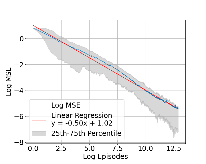
Figure 1: Log-log plot of MSE of learned $\phi_{1,n}$ in Algorithm 1

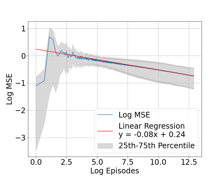
Figure 2: Log-log plot of MSE of learned $\phi_{1,n}$ in the benchmark algorithm

A comparison of regrets between Algorithms 1 and 2 is presented in Figures 4 and 4. The former yields a regret slope of around 0.73, which is close to the theoretical bound stipulated in Theorem 2 and superior to the slope of 0.88 achieved by the latter.

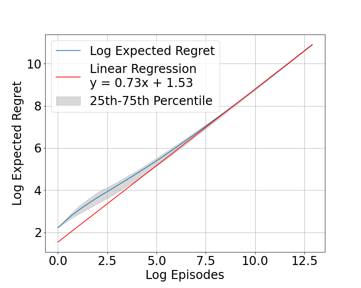
Figure 3: Log-log plot of the regret of Algorithm 1

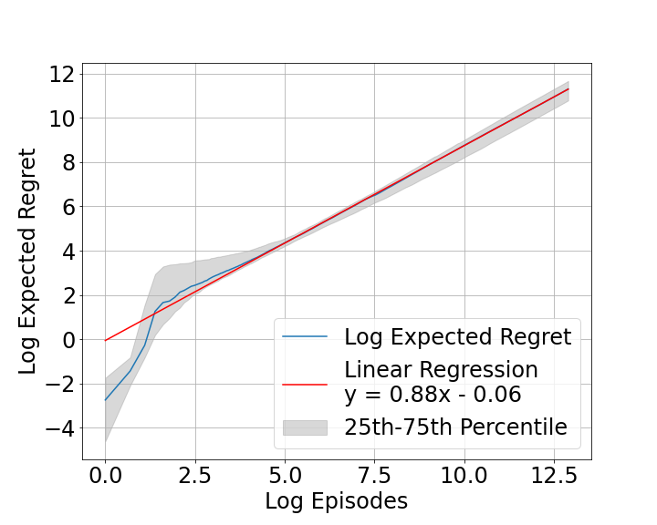
Figure 4: Log-log plot of the regret of the benchmark algorithm

These experimental results support the theoretical claims and demonstrate the outperformance of our RL-LQ algorithm compared with its model-based counterpart in terms of both the convergence rates of the policy parameters and the regret bounds.

6 Conclusions

This paper is the first to derive a convergence rate and a regret bound within the model-free framework of continuous-time entropy-regularized RL for controlled diffusion processes initiated by Wang et al., (2020). Here, by model-free, we mean that neither theory nor algorithm involves estimating model parameters. While it deals with the LQ case, it treats the case in which the diffusion term depends both on state and control, one that has not been studied in the RL literature to our best knowledge.

Note that the paper assumes scalar-valued states and controls for notational simplicity, though extending the results and algorithm to the multi-dimensional case presents no essential technical difficulty.

There are several limitations in the setting or results of the paper. First, the quadratic objective functional (2) has no running reward from controls, a key assumption needed to simplify our analysis so that it suffices to consider only (time-invariant) stationary policies. Second, we are unable to achieve a better sublinear regret, e.g., a square-root one, which is typical in episodic RL algorithms for tabular or linear MDPs. We are not certain whether that is due to our approach or it is more fundamental due to the diffusion nature of the system dynamics. Finally, extending the analysis to the non-LQ problems with general function approximations is an enormous open question. All these point to exciting research opportunities in the (hopefully near) future.

Appendix A A Proof of Theorem 1

Let $x_{n}=\{x_{n}(t):0\leq t\leq T\}$ be the sample state trajectory in the $n$-th iteration that follows the dynamics:

$$\mathrm{d}x_{n}(t)=(Ax_{n}(t)+Bu_{n}(t))\mathrm{d}t+(Cx_{n}(t)+Du_{n}(t))\mathrm{d}W_{n}(t),\quad 0\leq t\leq T,$$ (25)

where $W_{n}$ is a standard Brownian motion in the $n$-th iteration, and the policy $u_{n}(t)\mid x_{n}(t)\sim\mathcal{N}(\cdot|\phi_{1,n}x_{n}(t),\phi_{2,n})$ independent of $W_{n}(t)$.

Recall $Z_{1}(\cdot)$ defined by (17), and $Z_{1,n}(T)$ defined by (21) as the value of $Z_{1}(T)$ at the $n$-th iteration. Moreover, let $\hat{Z}_{1,n}(T)$ denote an empirical realization of $Z_{1,n}(T)$ observed in the algorithm iterations, which includes inherent random errors. The expectation of $Z_{1,n}(T)$ conditioned on the parameters is denoted by

$$h_{1}(\phi_{1,n},\phi_{2,n};\boldsymbol{\theta}_{n})=\mathbb{E}[Z_{1,n}(T)\mid\boldsymbol{\theta}_{n},\boldsymbol{\phi}_{n}],$$

and the noise contained in $\hat{Z}_{1,n}(T)$ is defined as

$$\xi_{1,n}=\hat{Z}_{1,n}(T)-h_{1}(\phi_{1,n},\phi_{2,n};\boldsymbol{\theta}_{n}).$$

Hence, the updating rule for $\phi_{1}$ is given by:

$$\phi_{1,n+1}=\Pi_{K_{1,n+1}}(\phi_{1,n}+a_{n}[h_{1}(\phi_{1,n},\phi_{2,n};\boldsymbol{\theta}_{n})+\xi_{1,n}]).$$ (26)

To prove Theorem 1, we need a series of lemmas to adapt the general stochastic approximation techniques and results (e.g. (Andradóttir,, 1995) and (Broadie et al.,, 2011)) to our specific setting.

A.1 Moment Estimates

Let $\{x^{\boldsymbol{\phi}}(t):0\leq t\leq T\}$ be the state process under the policy (14) following the dynamic (6). The following lemma gives some moment estimates of $x^{\boldsymbol{\phi}}(t)$ in terms of $\boldsymbol{\phi}$.

Lemma 1.

There exists a constant $c>0$ (that only depends on $A,B,C,D$) such that

$$\mathbb{E}[x^{\boldsymbol{\phi}}(t)]=x_{0}e^{(A+B\phi_{1})t},$$

$$\mathbb{E}[x^{\boldsymbol{\phi}}(t)^{2}] =D^{2}\phi_{2}\int_{0}^{t}e^{a(\phi_{1})(t-s)}\mathrm{d}s+x_{0}^{2}e^{a(\phi_{1})t},$$

where

$$a(\phi_{1})=2A+2B\phi_{1}+C^{2}+2CD\phi_{1}+D^{2}\phi_{1}^{2}.$$ (27)

Moreover, we have

$$\mathbb{E}[x^{\boldsymbol{\phi}}(t)^{2}]\leq c(1+|\phi_{2}|t)\exp{\{c|\phi_{1}|^{2}t\}},$$

$$\mathbb{E}[x^{\boldsymbol{\phi}}(t)^{4}]\leq c(1+|\phi_{2}|^{2}t)\exp{\{c|\phi_{1}|^{4}t\}},$$

$$\mathbb{E}[x^{\boldsymbol{\phi}}(t)^{6}]\leq c(1+|\phi_{2}|^{3}t)\exp{\{c|\phi_{1}|^{6}t\}}.$$

Proof.

We have

$$x^{\boldsymbol{\phi}}(t)=x(0) +\int_{0}^{t}\left(Ax^{\boldsymbol{\phi}}(s)+B\phi_{1}x^{\boldsymbol{\phi}}(s)\right)\mathrm{d}s$$

$$+\int_{0}^{t}\sqrt{C^{2}x^{\boldsymbol{\phi}}(s)^{2}+2CD\phi_{1}x^{\boldsymbol{\phi}}(s)^{2}+D^{2}(\phi_{1}^{2}x^{\boldsymbol{\phi}}(s)^{2}+\phi_{2})}\mathrm{d}W(s).$$

Taking expectation on both sides, we have

$$\mathbb{E}[x^{\boldsymbol{\phi}}(t)]=x_{0}+\int_{0}^{t}(A\mathbb{E}[x^{\boldsymbol{\phi}}(s)]+B\phi_{1}\mathbb{E}[x^{\boldsymbol{\phi}}(s)])\mathrm{d}s,$$

leading to

$$\mathbb{E}[x^{\boldsymbol{\phi}}(t)]=x_{0}e^{(A+B\phi_{1})t}.$$ (28)

Next, applying Ito’s formula to $x^{\boldsymbol{\phi}}(t)^{2}$ and taking expectation on both sides, we obtain

$$\mathbb{E}[x^{\boldsymbol{\phi}}(t)^{2}]=x_{0}^{2}+\int_{0}^{t}\left(a(\phi_{1})\mathbb{E}[x^{\boldsymbol{\phi}}(s)^{2}]+\phi_{2}D^{2}\right)\mathrm{d}s,$$

yielding

$$\mathbb{E}[x^{\boldsymbol{\phi}}(t)^{2}]=D^{2}\phi_{2}\int_{0}^{t}e^{a(\phi_{1})(t-s)}\mathrm{d}s+x_{0}^{2}e^{a(\phi_{1})t}.$$ (29)

Now we prove the inequality related to $\mathbb{E}[x^{\boldsymbol{\phi}}(t)^{6}]$. Hölder’s inequality yields

$$\mathbb{E}[x^{\boldsymbol{\phi}}(t)^{6}]$$

$$= \mathbb{E}\biggl{[}\biggl{(}x(0)+\int_{0}^{t}Ax^{\boldsymbol{\phi}}(s)+B\phi_{1}x^{\boldsymbol{\phi}}(s)\mathrm{d}s$$

$$\quad+\int_{0}^{t}\sqrt{C^{2}x^{\boldsymbol{\phi}}(s)^{2}+2CD\phi_{1}x^{\boldsymbol{\phi}}(s)^{2}+D^{2}(\phi_{1}^{2}x^{\boldsymbol{\phi}}(s)^{2}+\phi_{2})}\mathrm{d}W(s)\biggl{)}^{6}\biggl{]}$$

$$\leq cx_{0}^{6}+c\mathbb{E}\biggl{[}\biggl{(}\int_{0}^{t}Ax^{\boldsymbol{\phi}}(s)+B\phi_{1}x^{\boldsymbol{\phi}}(s)\mathrm{d}s\biggl{)}^{6}\biggl{]}$$

$$+c\mathbb{E}\biggl{[}\biggl{(}\int_{0}^{t}\sqrt{C^{2}x^{\boldsymbol{\phi}}(s)^{2}+2CD\phi_{1}x^{\boldsymbol{\phi}}(s)^{2}+D^{2}(\phi_{1}^{2}x^{\boldsymbol{\phi}}(s)^{2}+\phi_{2})}\mathrm{d}W(s)\biggl{)}^{6}\biggl{]}$$

$$\leq cx_{0}^{6}+c(A+B\phi_{1})^{6}\mathbb{E}\biggl{[}\biggl{(}\int_{0}^{t}x^{\boldsymbol{\phi}}(s)\mathrm{d}s\biggl{)}^{6}\biggl{]}$$

$$+c\mathbb{E}\biggl{[}\biggl{(}\int_{0}^{t}C^{2}x^{\boldsymbol{\phi}}(s)^{2}+2CD\phi_{1}x^{\boldsymbol{\phi}}(s)^{2}+D^{2}(\phi_{1}^{2}x^{\boldsymbol{\phi}}(s)^{2}+\phi_{2})\mathrm{d}s\biggl{)}^{3}\biggl{]}$$

$$\leq cx_{0}^{6}+c(1+|\phi_{1}|^{6})\mathbb{E}\biggl{[}\int_{0}^{t}x^{\boldsymbol{\phi}}(s)^{6}\mathrm{d}s\biggl{]}+c\mathbb{E}\biggl{[}\int_{0}^{t}(1+|\phi_{1}|^{6})x^{\boldsymbol{\phi}}(s)^{6}+|\phi_{2}|^{3}\mathrm{d}s\biggl{]}.$$

It follows from Grönwall’s inequality that

$$\mathbb{E}[x^{\boldsymbol{\phi}}(t)^{6}]\leq c(1+|\phi_{2}|^{3}t)\exp{\{\int_{0}^{t}c(1+|\phi_{1}|^{6})\mathrm{d}s\}}$$

$$= c(1+|\phi_{2}|^{3}t)\exp{\{c(1+|\phi_{1}|^{6})t\}}$$

$$\leq ce^{cT}(1+|\phi_{2}|^{3}t)\exp{\{c|\phi_{1}|^{6}t\}}.$$

The proofs for the inequalities of $\mathbb{E}[x^{\boldsymbol{\phi}}(t)^{2}]$ and $\mathbb{E}[x^{\boldsymbol{\phi}}(t)^{4}]$ are similar. ∎

The next lemma concerns the variance of the increment $Z_{1,n}(T)$.

Lemma 2.

There exists a constant $c>0$ that depends only on the model primitives such that

$$\operatorname{Var}\left(Z_{1,n}(T)\Big{|}\boldsymbol{\theta}_{n},\phi_{1,n},\phi_{2,n}\right)\leq cb_{n}\left(1+|\phi_{1,n}|^{8}+(\log b_{n})^{8}\right)\exp{\{c|\phi_{1,n}|^{6}\}}.$$ (30)

Proof.

Applying Ito’s lemma to the process $J\left(t,x_{n}(t);\boldsymbol{\theta}_{n}\right)$, where $x_{n}$ follows (25), we have

$$\mathrm{d}J\left(t,x_{n}(t);\boldsymbol{\theta}_{n}\right)= \biggl{(}-\frac{1}{2}k_{1}^{\prime}(t;\boldsymbol{\theta}_{n})x_{n}(t)^{2}+k_{3}^{\prime}(t;\boldsymbol{\theta}_{n})-(Ax_{n}(t)+Bu_{n}(t))k_{1}(t;\boldsymbol{\theta}_{n})x_{n}(t)$$

$$-\frac{(Cx_{n}(t)+Du_{n}(t))^{2}}{2}k_{1}(t;\boldsymbol{\theta}_{n})\biggl{)}\mathrm{d}t$$

$$-\biggl{(}(Cx_{n}(t)+Du_{n}(t))k_{1}(t;\boldsymbol{\theta}_{n})x_{n}(t)\biggl{)}\mathrm{d}W_{n}(t).$$

In addition,

$${p}(t,\boldsymbol{\phi}_{n})=\log(\sqrt{2\pi e\phi_{2,n}})=\frac{1}{2}\log(\phi_{2,n})+\frac{1}{2}\log(2\pi e).$$

Hence

$$\mathrm{d}Z_{1,n}(t)= \frac{(u_{n}(t)-\phi_{1,n}x_{n}(t))x_{n}(t)}{\phi_{2,n}}\biggl{[}\biggl{(}-\frac{1}{2}k_{1}^{\prime}(t;\boldsymbol{\theta}_{n})x_{n}(t)^{2}+k_{3}^{\prime}(t;\boldsymbol{\theta}_{n})$$ (31)

$$-(Ax_{n}(t)+Bu_{n}(t))k_{1}(t;\boldsymbol{\theta}_{n})x_{n}(t)-\frac{(Cx_{n}(t)+Du_{n}(t))^{2}}{2}k_{1}(t;\boldsymbol{\theta}_{n})\biggl{)}\mathrm{d}t$$

$$-\biggl{(}(Cx_{n}(t)+Du_{n}(t))k_{1}(t;\boldsymbol{\theta}_{n})x_{n}(t)\biggl{)}\mathrm{d}W_{n}(t)-\frac{1}{2}Qx_{n}(t)^{2}\mathrm{d}t$$

$$+\gamma\biggl{(}\frac{1}{2}\log(\phi_{2,n})+\frac{1}{2}\log(2\pi e)\biggl{)}\mathrm{d}t\biggl{]}$$

$$= \frac{(u_{n}(t)-\phi_{1,n}x_{n}(t))x_{n}(t)}{\phi_{2,n}}\biggl{[}\biggl{(}-\frac{1}{2}k_{1}^{\prime}(t;\boldsymbol{\theta}_{n})x_{n}(t)^{2}+k_{3}^{\prime}(t;\boldsymbol{\theta}_{n})$$

$$-(Ax_{n}(t)+Bu_{n}(t))k_{1}(t;\boldsymbol{\theta}_{n})x_{n}(t)-\frac{(Cx_{n}(t)+Du_{n}(t))^{2}}{2}k_{1}(t;\boldsymbol{\theta}_{n})\biggl{)}$$

$$-\frac{1}{2}Qx_{n}(t)^{2}+\gamma\biggl{(}\frac{1}{2}\log(\phi_{2,n})+\frac{1}{2}\log(2\pi e)\biggl{)}\biggl{]}\mathrm{d}t$$

$$-\frac{(u_{n}(t)-\phi_{1,n}x_{n}(t))x_{n}(t)}{\phi_{2,n}}\biggl{(}(Cx_{n}(t)+Du_{n}(t))k_{1}(t;\boldsymbol{\theta}_{n})x_{n}(t)\biggl{)}\mathrm{d}W_{n}(t)$$

$$\triangleq Z_{1,n}^{(1)}(t)\mathrm{d}t+Z_{1,n}^{(2)}(t)\mathrm{d}W_{n}(t).$$

We now estimate

$$\mathbb{E}[|Z_{1,n}^{(1)}(t)|^{2}|\boldsymbol{\theta}_{n},\phi_{1,n},\phi_{2,n},x_{n}(t)]\leq c\biggl{[}(1+|\phi_{1,n}|^{4})|\phi_{2,n}|^{-1}x_{n}(t)^{6}+(1+|\phi_{1,n}|^{2})x_{n}(t)^{4}$$

$$+(1+|\phi_{2,n}|^{2}+(\log(|\phi_{2,n}|))^{4})|\phi_{2,n}|^{-1}x_{n}(t)^{2}\biggl{]},$$

and

$$\mathbb{E}[|Z_{1,n}^{(2)}(t)|^{2}|\boldsymbol{\theta}_{n},\phi_{1,n},\phi_{2,n},x_{n}(t)]\leq c\biggl{[}1+|\phi_{2,n}|^{-1}(1+|\phi_{1,n}|^{2})x_{n}(t)^{6}+x_{n}(t)^{4}\biggl{]}.$$

By Lemma 1, taking expectations in the above with respect to $x_{n}(t)$, we deduce

$$\mathbb{E}[|Z_{1,n}^{(1)}(t)|^{2}+|Z_{1,n}^{(2)}(t)|^{2}|\boldsymbol{\theta}_{n},\phi_{1,n},\phi_{2,n}]$$ (32)

$$\leq c\biggl{[}(1+|\phi_{1,n}|^{4})|\phi_{2,n}|^{-1}(1+|\phi_{2,n}t|^{3})\exp{\{c|\phi_{1,n}|^{6}t\}}$$

$$+(1+|\phi_{1,n}|^{2})(1+|\phi_{2,n}t|^{2})\exp{\{c|\phi_{1,n}|^{4}t\}}$$

$$+(1+|\phi_{2,n}|^{2}+(\log(|\phi_{2,n}|))^{4})|\phi_{2,n}|^{-1}(1+|\phi_{2,n}t|)\exp{\{c|\phi_{1,n}|^{2}t\}}\biggl{]}.$$

Recalling that $\phi_{2,n}=\frac{1}{b_{n}}$ set in Algorithm 1, we arrive at (30).∎

A.2 Mean Increment

We now analyze the mean increment $h_{1}(\phi_{1,n},\phi_{2,n};\boldsymbol{\theta}_{n})$ in the updating rule (26). First, note that $\int_{0}^{\cdot}Z_{1,n}^{(2)}(t)\mathrm{d}W_{n}(t)$ is a martingale by virtue of Lemma 1 and (32). Taking integration and expectation in (31), we get

$$\mathbb{E}[Z_{1,n}(s)] =\mathbb{E}\int_{0}^{s}\frac{1}{2\phi_{2,n}}x_{n}(t)[-2Bk_{1}(t;\boldsymbol{\theta}_{n})x_{n}(t)(u_{n}(t)-\phi_{1,n}x_{n}(t))^{2}$$ (33)

$$\quad-2CDk_{1}(t;\boldsymbol{\theta}_{n})x_{n}(t)(u_{n}(t)-\phi_{1,n}x_{n}(t))$$

$$\quad-2D^{2}k_{1}(t;\boldsymbol{\theta}_{n})x_{n}(t)(u_{n}(t)-\phi_{1,n}x_{n}(t))^{2}]\mathrm{d}t$$

$$=-\int_{0}^{s}k_{1}(t;\boldsymbol{\theta}_{n})(B+CD+D^{2}\phi_{1,n})\mathbb{E}[x_{n}(t)^{2}]\mathrm{d}t,\;\;0\leq s\leq T.$$

Hence

$$h_{1}(\phi_{1,n},\phi_{2,n};\boldsymbol{\theta}_{n}) =-(B+CD+D^{2}\phi_{1,n})\int_{0}^{T}k_{1}(t;\boldsymbol{\theta}_{n})\mathbb{E}[x_{n}(t)^{2}]\mathrm{d}t$$ (34)

$$=-(\phi_{1,n}-\phi_{1}^{*})l(\phi_{1,n},\phi_{2,n};\boldsymbol{\theta}_{n}),$$

where

$$l(\phi_{1,n},\phi_{2,n};\boldsymbol{\theta}_{n})=D^{2}\int_{0}^{T}k_{1}(t;\boldsymbol{\theta}_{n})\mathbb{E}[x_{n}(t)^{2}]\mathrm{d}t.$$ (35)

Next we study $h_{1}(\phi_{1,n},\phi_{2,n};\boldsymbol{\theta}_{n})$. It follows from (27) that $a(\phi_{1})$ is a quadratic function of $\phi_{1}$ and $a(\phi_{1})\geq-\frac{B^{2}+2BCD-2AD^{2}}{D^{2}}$. Hence, by (29), we have

$$\mathbb{E}[x_{n}(t)^{2}] =D^{2}\phi_{2,n}\int_{0}^{t}e^{a(\phi_{1,n})(t-s)}\mathrm{d}s+x_{0}^{2}e^{a(\phi_{1,n})t}$$ (36)

$$\geq x_{0}^{2}e^{a(\phi_{1,n})t}\geq c$$

where $c>0$ is a constant independent of $n$. Thus,

$$l(\phi_{1,n},\phi_{2,n};\boldsymbol{\theta}_{n}) =D^{2}\int_{0}^{T}k_{1}(t;\boldsymbol{\theta}_{n})\mathbb{E}[x_{n}(t)^{2}]\mathrm{d}t$$ (37)

$$\geq D^{2}\int_{0}^{T}(1/c_{2})c\mathrm{d}t=D^{2}(1/c_{2})cT \geq\bar{c}$$

where $0<\bar{c}<1$ is a constant independent of $n$.

On the other hand, since $a(\phi_{1})$ is a quadratic function of $\phi_{1}$, we have

$$|a(\phi_{1})|\leq c(1+|\phi_{1}|^{2}),\;\;\forall\phi_{1}\in\mathbb{R},$$

for some constant $c>0$. So

$$\mathbb{E}[x_{n}(t)^{2}] =D^{2}\phi_{2,n}\int_{0}^{t}e^{a(\phi_{1,n})(t-s)}\mathrm{d}s+x_{0}^{2}e^{a(\phi_{1,n})t}$$

$$\leq c(1+|\phi_{2,n}|)e^{c|\phi_{1,n}|^{2}T},$$

leading to

$$l(\phi_{1,n},\phi_{2,n};\boldsymbol{\theta}_{n}) =D^{2}\int_{0}^{T}k_{1}(t;\boldsymbol{\theta}_{n})\mathbb{E}[x_{n}(t)^{2}]\mathrm{d}t$$

$$\leq D^{2}c_{2}Tc(1+|\phi_{2,n}|)e^{c|\phi_{1,n}|^{2}T}.$$

Recalling that $\phi_{2,n}=\frac{1}{b_{n}}$, we arrive at

$$|h_{1}(\phi_{1,n},\phi_{2,n};\boldsymbol{\theta}_{n})| =|\phi_{1,n}-\phi_{1}^{*}|l(\phi_{1,n},\phi_{2,n};\boldsymbol{\theta}_{n})$$ (38)

$$\leq c(1+|\phi_{1,n}|)e^{c|\phi_{1,n}|^{2}}$$

for some constant $c>0$.

A.3 Almost Sure Convergence of $\phi_{1,n}$

We first prove the almost sure convergence of $\phi_{1,n}$. Part (a) of Theorem 1 is a special case of the following result when $\beta_{1,n}=0$.

Theorem 3.

Assume the noise term $\xi_{1,n}$ satisfies $\mathbb{E}\left[\xi_{1,n}\Big{|}\mathcal{G}_{n}\right]=\beta_{1,n}$ and

$$\mathbb{E}\left[\left|\xi_{1,n}-\beta_{1,n}\right|^{2}\Big{|}\mathcal{G}_{n}\right]\leq cb_{n}(1+|\phi_{1,n}|^{8}+(\log b_{n})^{8})\exp{\{c|\phi_{1,n}|^{6}\}},$$ (39)

where $c>0$ is a constant independent of $n$, and $\{\mathcal{G}_{n}\}$ is the filtration generated by $\{\boldsymbol{\theta}_{m},\phi_{1,m},\phi_{2,m},m=0,1,2,...,n\}$. Moreover, assume

$$(i) \quad 0<a_{n}\leq 1\text{ for all }n,\quad\sum_{n}a_{n}=\infty,\quad\sum_{n}a_{n}|\beta_{1,n}|<\infty;$$ (40)

$$(ii) \quad c_{1,n}\uparrow\infty,\quad\sum_{n}a_{n}^{2}b_{n}^{q}(\log b_{n})^{q_{2}}e^{cc_{1,n}^{q_{3}}}<\infty$$

$$\quad\text{for any }c>0\text{, }0\leq q\leq 1\text{ , }0\leq q_{2}\leq 8\text{ and }0\leq q_{3}\leq 6;$$

$$(iii) \quad b_{n}\geq 1\text{ for all }n,\quad b_{n}\uparrow\infty.$$

Then $\phi_{1,n}$ almost surely converges to the unique equilibrium point $\phi_{1}^{*}=-\frac{B+CD}{D^{2}}$ .

Proof.

The main idea is to derive inductive upper bounds of $|\phi_{1,n}-\phi_{1}^{*}|^{2}$, namely, we will bound $|\phi_{1,n+1}-\phi_{1}^{*}|^{2}$ in terms of $|\phi_{1,n}-\phi_{1}^{*}|^{2}$.

First, for any closed, convex set $K\subset\mathbb{R}$ and $x\in K,y\in\mathbb{R}$, it follows from a property of projection that the function $f(t)=|t\Pi_{K}(y)+(1-t)x-y|^{2}$, $t\in\mathbb{R}$, achieves minimum at $t=1$. The first-order condition at $t=1$ then yields

$$2|\Pi_{K}(y)-y|^{2}-2\langle\Pi_{K}(y)-y,x-y\rangle=0.$$

Therefore,

$$|\Pi_{K}(y)-x|^{2}= |\Pi_{K}(y)-y+y-x|^{2}=|y-x|^{2}+|\Pi_{K}(y)-y|^{2}+2\langle\Pi_{K}(y)-y,y-x\rangle$$

$$= |y-x|^{2}-|\Pi_{K}(y)-y|^{2}\leq|y-x|^{2}.$$

Taking $n$ sufficiently large such that $\phi_{1}^{*}\in K_{1,n+1}$, we have

$$|\phi_{1,n+1}-\phi_{1}^{*}|^{2}\leq|\phi_{1,n}+a_{n}[h_{1}(\phi_{1,n},\phi_{2,n};\boldsymbol{\theta}_{n})+\xi_{1,n}]-\phi_{1}^{*}|^{2}.$$

Denoting $U_{1,n}=\phi_{1,n}-\phi_{1}^{*}$, we deduce

$$\mathbb{E}\left[|U_{1,n+1}|^{2}\Big{|}\mathcal{G}_{n}\right]$$

$$\leq \mathbb{E}\left[|U_{1,n}+a_{n}[h_{1}(\phi_{1,n},\phi_{2,n};\boldsymbol{\theta}_{n})+\xi_{1,n}]|^{2}\Big{|}\mathcal{G}_{n}\right]$$

$$= |U_{1,n}|^{2}+2a_{n}\langle U_{1,n},h_{1}(\phi_{1,n},\phi_{2,n};\boldsymbol{\theta}_{n})+\beta_{1,n}\rangle+a_{n}^{2}\mathbb{E}\left[|h_{1}(\phi_{1,n},\phi_{2,n};\boldsymbol{\theta}_{n})+\xi_{1,n}|^{2}\Big{|}\mathcal{G}_{n}\right]$$

$$= |U_{1,n}|^{2}+2a_{n}\langle U_{1,n},h_{1}(\phi_{1,n},\phi_{2,n};\boldsymbol{\theta}_{n})+\beta_{1,n}\rangle$$

$$+a_{n}^{2}\mathbb{E}\left[|h_{1}(\phi_{1,n},\phi_{2,n};\boldsymbol{\theta}_{n})+(\xi_{1,n}-\beta_{1,n})+\beta_{1,n}|^{2}\Big{|}\mathcal{G}_{n}\right]$$

$$\leq |U_{1,n}|^{2}+2a_{n}\langle U_{1,n},h_{1}(\phi_{1,n},\phi_{2,n};\boldsymbol{\theta}_{n})\rangle+2a_{n}|\beta_{1,n}||U_{1,n}|$$

$$+3a_{n}^{2}\left(|h_{1}(\phi_{1,n},\phi_{2,n};\boldsymbol{\theta}_{n})|^{2}+|\beta_{1,n}|^{2}+\mathbb{E}\left[\left|\xi_{1,n}-\beta_{1,n}\right|^{2}\Big{|}\mathcal{G}_{n}\right]\right)$$

$$\leq |U_{1,n}|^{2}+2a_{n}\langle U_{1,n},h_{1}(\phi_{1,n},\phi_{2,n};\boldsymbol{\theta}_{n})\rangle+a_{n}|\beta_{1,n}|(1+|U_{1,n}|^{2})$$

$$+3a_{n}^{2}\left(|h_{1}(\phi_{1,n},\phi_{2,n};\boldsymbol{\theta}_{n})|^{2}+|\beta_{1,n}|^{2}+\mathbb{E}\left[\left|\xi_{1,n}-\beta_{1,n}\right|^{2}\Big{|}\mathcal{G}_{n}\right]\right).$$

Recall that $|\phi_{1,n}|\leq c_{1,n}$ almost surely. By (38), we have

$$|h_{1}(\phi_{1,n},\phi_{2,n};\boldsymbol{\theta}_{n})|^{2}\leq c(1+|\phi_{1,n}|)^{2}e^{2c|\phi_{1,n}|^{2}}\leq c(1+c_{1,n}^{2})e^{cc_{1,n}^{2}}.$$

In addition, the assumption (39) yields

$$\mathbb{E}\left[\left|\xi_{1,n}-\beta_{1,n}\right|^{2}\Big{|}\mathcal{G}_{n}\right]\leq cb_{n}(1+|\phi_{1,n}|^{8}+(\log b_{n})^{8})\exp{\{c|\phi_{1,n}|^{6}\}}$$

$$\leq cb_{n}(1+c_{1,n}^{8}+(\log b_{n})^{8})\exp{\{cc_{1,n}^{6}\}}.$$

Therefore,

$$\mathbb{E}\left[|U_{1,n+1}|^{2}\Big{|}\mathcal{G}_{n}\right]$$

$$\leq |U_{1,n}|^{2}+2a_{n}\langle U_{1,n},h_{1}(\phi_{1,n},\phi_{2,n};\boldsymbol{\theta}_{n})\rangle+a_{n}|\beta_{1,n}|(1+|U_{1,n}|^{2})$$

$$+3a_{n}^{2}\left(|h_{1}(\phi_{1,n},\phi_{2,n};\boldsymbol{\theta}_{n})|^{2}+|\beta_{1,n}|^{2}+\mathbb{E}\left[\left|\xi_{1,n}-\beta_{1,n}\right|^{2}\Big{|}\mathcal{G}_{n}\right]\right)$$

$$\leq (1+a_{n}|\beta_{1,n}|)|U_{1,n}|^{2}+2a_{n}\langle U_{1,n},h_{1}(\phi_{1,n},\phi_{2,n};\boldsymbol{\theta}_{n})\rangle+a_{n}|\beta_{1,n}|$$

$$+3a_{n}^{2}\bigg{(}c(1+c_{1,n}^{2})e^{cc_{1,n}^{2}}+|\beta_{1,n}|^{2}+cb_{n}(1+c_{1,n}^{8}+(\log b_{n})^{8})\exp{\{cc_{1,n}^{6}\}}\bigg{)}$$

$$= :(1+\kappa_{1,n})|U_{1,n}|^{2}-\zeta_{1,n}+\eta_{1,n},$$

where $\kappa_{1,n}=a_{n}|\beta_{1,n}|$, $\zeta_{1,n}=-2a_{n}\langle U_{1,n},h_{1}(\phi_{1,n},\phi_{2,n};\boldsymbol{\theta}_{n})\rangle$, and

$$\eta_{1,n}= a_{n}|\beta_{1,n}|+3a_{n}^{2}\bigg{(}c(1+c_{1,n}^{2})e^{cc_{1,n}^{2}}+|\beta_{1,n}|^{2}+cb_{n}(1+c_{1,n}^{8}+(\log b_{n})^{8})\exp{\{cc_{1,n}^{6}\}}\bigg{)}.$$ (41)

By assumptions (i)-(ii) of (40), we know $\sum\kappa_{1,n}<\infty$ and $\sum\eta_{1,n}<\infty$. It then follows from (Robbins and Siegmund,, 1971, Theorem 1) that $\left|U_{1,n}\right|^{2}$ converges to a finite limit and $\sum\zeta_{1,n}<\infty$ almost surely.

It remains to show $|U_{1,n}|\to 0$ almost surely. It follows from (35) and (37) that

$$\zeta_{1,n} =-2a_{n}\langle U_{1,n},h_{1}(\phi_{1,n},\phi_{2,n};\boldsymbol{\theta}_{n})\rangle$$

$$=2a_{n}(\phi_{1,n}-\phi_{1}^{*})^{2}l(\phi_{1,n},\phi_{2,n};\boldsymbol{\theta}_{n})$$

$$\geq 2\bar{c}a_{n}(\phi_{1,n}-\phi_{1}^{*})^{2}.$$

Now, suppose $|U_{1,n}|\nrightarrow 0$ almost surely. Then there exists a set $Z\in\mathcal{F}$ with $\mathbb{P}(Z)>0$ so that for every $\omega\in Z$, there is $\delta(\omega)>0$ such that $|U_{1,n}|=|\phi_{1,n}-\phi_{1}^{*}|\geq\delta(\omega)>0$ for sufficiently large $n$. Thus,

$$\sum\zeta_{1,n}\geq\sum 2\bar{c}a_{n}(\phi_{1,n}-\phi_{1}^{*})^{2}\geq 2\bar{c}\delta(\omega)^{2}\sum a_{n}=\infty.$$

This is a contradiction. Therefore, we have proved that $|U_{1,n}|$ converges to 0 almost surely, or $\phi_{1,n}$ converges to $\phi_{1}^{*}=-\frac{B+CD}{D^{2}}$ almost surely. ∎

Remark 1.

A typical choice satisfying the assumptions in (40) is $a_{n}=1\wedge\frac{\alpha^{\frac{3}{4}}}{(n+\beta)^{\frac{3}{4}}}$, where constants $\alpha>0$, $\beta>0$. $b_{n}=1\vee\frac{(n+\beta)^{\frac{1}{4}}}{\alpha^{\frac{1}{4}}},c_{1,n}=1\vee(\log\log n)^{\frac{1}{6}},\beta_{1,n}=0$ or $\beta_{1,n}=n^{-\frac{3}{8}}$. This is because $\sum\frac{1}{n}=\infty$, and $\sum\frac{(\log n)^{p}(\log\log n)^{q}}{n^{r}}<\infty$, for any $p,q>0$ and $r>1$.

A.4 Mean-Squared Error of $\phi_{1,n}-\phi_{1}^{*}$

In this section, we establish the convergence rate of $\phi_{1,n}$ to $\phi_{1}^{*}$ stipulated in part (b) of Theorem 1.

The following lemma shows a general recursive relation satisfied by some sequences of learning rates.

Lemma 3.

For any $w>0$, there exists positive numbers $\alpha>\frac{1}{w}$ and $\beta\geq\max(\frac{1}{w\alpha-1},w^{2}\alpha^{3})$ such that the sequence $a_{n}=\frac{\alpha^{\frac{3}{4}}}{(n+\beta)^{\frac{3}{4}}}$ satisfies $a_{n}\leq a_{n+1}(1+wa_{n+1})$ for all $n\geq 0$.

Proof.

We have the following equivalences:

$$a_{n}\leq a_{n+1}(1+wa_{n+1})$$ (42)

$$\Leftrightarrow \frac{\alpha^{\frac{3}{4}}}{(n+\beta)^{\frac{3}{4}}}\leq\frac{\alpha^{\frac{3}{4}}}{(n+1+\beta)^{\frac{3}{4}}}+w\left(\frac{\alpha}{n+1+\beta}\right)^{\frac{2}{3}}$$

$$\Leftrightarrow (n+\beta+1)^{\frac{3}{4}}-(n+\beta)^{\frac{3}{4}}\leq w\alpha^{\frac{3}{4}}\biggl{(}\frac{n+\beta}{n+\beta+1}\biggl{)}^{\frac{3}{4}}.$$

Consider the last inequality in (42) and notice that the left hand side is a decreasing function of $n$ and the right hand side is an increasing function of $n$. So to show that this inequality is true for all $n$, it is sufficient to show that it is true when $n=0$, which is

$$(\beta+1)^{\frac{3}{4}}-\beta^{\frac{3}{4}}\leq w\alpha^{\frac{3}{4}}\frac{\beta^{\frac{3}{4}}}{(\beta+1)^{\frac{3}{4}}}.$$ (43)

To this end, it follows from $\beta\geq w^{2}\alpha^{3}$ and $w\alpha\beta\geq\beta+1$ that

$$w\beta^{4}\geq w^{3}\alpha^{3}\beta^{3}\geq(\beta+1)^{3}.$$

Hence

$$w^{\frac{1}{4}}\frac{\beta^{\frac{3}{4}}}{(\beta+1)^{\frac{3}{4}}}\geq\frac{3}{4}\beta^{-\frac{1}{4}}\geq(\beta+1)^{\frac{3}{4}}-\beta^{\frac{3}{4}},$$

where the last inequality is due to the mean value theorem. Now the desired inequality (43) follows from the fact that $\alpha>\frac{1}{w}$. ∎

The following result covers part (b) of Theorem 1 as a special case.

Theorem 4.

Under the assumption of Theorem 3, if the sequence $\{a_{n}\}$ further satisfies

$$a_{n}\leq a_{n+1}(1+wa_{n+1})$$

for some sufficiently small constant $w>0$ and $\{\frac{b_{n}}{a_{n}}|\beta_{1,n}|^{2}\}$ is increasing in $n$, then there exists an increasing sequence $\{\hat{\eta}_{1,n}\}$ and a constant ${c}^{\prime}>0$ such that

$$\mathbb{E}[|\phi_{1,n+1}-\phi_{1}^{*}|^{2}]\leq{c}^{\prime}a_{n}\hat{\eta}_{1,n}.$$

In particular, if we set the parameters $a_{n},b_{n},c_{1,n},\beta_{1,n}$ as in Remark 1, then

$$\mathbb{E}[|\phi_{1,n+1}-\phi_{1}^{*}|^{2}]\leq c\frac{(1\vee\log n)^{p}(1\vee\log\log n)^{\frac{4}{3}}}{n^{\frac{1}{2}}}$$

for any $n$, where $c$ and $p$ are positive constants that only depend on model primitives.

Proof.

Denote $n_{0}=\inf\{n\geq 0:\phi_{1}^{*}\in K_{1,n+1}\}$ and $U_{1,n}=\phi_{1,n}-\phi_{1}^{*}$. It follows from (34) and (37) that

$$U_{1,n}h_{1}(\phi_{1,n},\phi_{2,n};\boldsymbol{\theta}_{n})=-U_{1,n}^{2}l(\phi_{1,n},\phi_{2,n};\boldsymbol{\theta}_{n})\rangle\leq-\bar{c}|U_{1,n}|^{2}.$$ (44)

When $n\geq n_{0}$, this together with a similar argument to the proof of Theorem 3 yields

$$\mathbb{E}\left[|U_{1,n+1}|^{2}\Big{|}\mathcal{G}_{n}\right]$$ (45)

$$\leq |U_{1,n}|^{2}+2a_{n}U_{1,n}h_{1}(\phi_{1,n},\phi_{2,n};\boldsymbol{\theta}_{n})+2a_{n}|\beta_{1,n}||U_{1,n}|$$

$$+3a_{n}^{2}\left(|h_{1}(\phi_{1,n},\phi_{2,n};\boldsymbol{\theta}_{n})|^{2}+|\beta_{1,n}|^{2}+\mathbb{E}\left[\left|\xi_{1,n}-\beta_{1,n}\right|^{2}\Big{|}\mathcal{G}_{n}\right]\right)$$

$$\leq |U_{1,n}|^{2}-2a_{n}\bar{c}|U_{1,n}|^{2}+2a_{n}|\beta_{1,n}||U_{1,n}|$$

$$+3a_{n}^{2}\left(|h_{1}(\phi_{1,n},\phi_{2,n};\boldsymbol{\theta}_{n})|^{2}+|\beta_{1,n}|^{2}+\mathbb{E}\left[\left|\xi_{1,n}-\beta_{1,n}\right|^{2}\Big{|}\mathcal{G}_{n}\right]\right)$$

$$\leq |U_{1,n}|^{2}-2a_{n}\bar{c}|U_{1,n}|^{2}+a_{n}(\frac{1}{\bar{c}}|\beta_{1,n}|^{2}+\bar{c}|U_{1,n}|^{2})$$

$$+3a_{n}^{2}\left(|h_{1}(\phi_{1,n},\phi_{2,n};\boldsymbol{\theta}_{n})|^{2}+|\beta_{1,n}|^{2}+\mathbb{E}\left[\left|\xi_{1,n}-\beta_{1,n}\right|^{2}\Big{|}\mathcal{G}_{n}\right]\right)$$

$$= (1-\bar{c}a_{n})|U_{1,n}|^{2}+3a_{n}^{2}\bigg{(}|h_{1}(\phi_{1,n},\phi_{2,n};\boldsymbol{\theta}_{n})|^{2}+(1+\frac{1}{3\bar{c}a_{n}})|\beta_{1,n}|^{2}$$

$$+\mathbb{E}\left[\left|\xi_{1,n}-\beta_{1,n}\right|^{2}\Big{|}\mathcal{G}_{n}\right]\bigg{)}.$$

Now, by the proof of Theorem 3,

$$|h_{1}(\phi_{1,n},\phi_{2,n};\boldsymbol{\theta}_{n})|^{2}+\mathbb{E}\left[\left|\xi_{1,n}-\beta_{1,n}\right|^{2}\Big{|}\mathcal{G}_{n}\right]$$

$$\leq c\biggl{(}(1+c_{1,n}^{2})e^{cc_{1,n}^{2}}+b_{n}(1+c_{1,n}^{8}+(\log b_{n})^{8})\exp{\{cc_{1,n}^{6}\}}\biggl{)}$$

$$\leq cb_{n}(1+c_{1,n}^{8}+(\log b_{n})^{8})\exp{\{cc_{1,n}^{6}\}}.$$

Moreover, the assumptions in (40) imply that $(1+\frac{1}{3\bar{c}a_{n}})|\beta_{1,n}|^{2}\leq c\frac{b_{n}}{a_{n}}|\beta_{1,n}|^{2}$ for some constant $c>0$. When $n\geq n_{0}$, it follows from (45) that

$$\mathbb{E}\left[|U_{1,n+1}|^{2}\Big{|}\mathcal{G}_{n}\right]\leq(1-\bar{c}a_{n})|U_{1,n}|^{2}+3a_{n}^{2}\hat{\eta}_{1,n},$$

where

$$\hat{\eta}_{1,n}= cb_{n}(1+c_{1,n}^{8}+(\log b_{n})^{8}+\frac{|\beta_{1,n}|^{2}}{a_{n}})\exp{\{cc_{1,n}^{6}\}},$$ (46)

which is monotonically increasing because so are $c_{1,n}$, $b_{n}$ and $\frac{b_{n}}{a_{n}}|\beta_{1,n}|^{2}$ by the assumptions. Taking expectation on both sides of the above and denoting $\rho_{n}=\mathbb{E}[|U_{1,n}|^{2}]$, we get

$$\rho_{n+1}\leq(1-\bar{c}a_{n})\rho_{n}+3a_{n}^{2}\hat{\eta}_{1,n}$$ (47)

when $n\geq n_{0}$.

Next, we show $\rho_{n+1}\leq c^{\prime}a_{n}\hat{\eta}_{1,n}$ for all $n\geq 0$ by induction, where $c^{\prime}=max\{\frac{\rho_{1}}{a_{0}\hat{\eta}_{1,0}},\frac{\rho_{2}}{a_{1}\hat{\eta}_{1,1}},\cdots,\frac{\rho_{n_{0}+1}}{a_{n_{0}}\hat{\eta}_{1,{n_{0}}}},\frac{3}{\bar{c}}\}+1$. Indeed, it is true when $n\leq n_{0}$. Assume that $\rho_{k+1}\leq c^{\prime}a_{k}\hat{\eta}_{1,k}$ is true for $n_{0}\leq k\leq n-1$. Then (47) yields

$$\rho_{n+1} \leq(1-\bar{c}a_{n})\rho_{n}+3a_{n}^{2}\hat{\eta}_{1,n}$$

$$\leq(1-\bar{c}a_{n})c^{\prime}a_{n-1}\hat{\eta}_{1,n-1}+3a_{n}^{2}\hat{\eta}_{1,n}$$

$$\leq(1-\bar{c}a_{n})c^{\prime}a_{n}(1+wa_{n})\hat{\eta}_{1,n}+3a_{n}^{2}\hat{\eta}_{1,n}$$

$$=c^{\prime}a_{n}\hat{\eta}_{1,n}+c^{\prime}\hat{\eta}_{1,n}a_{n}^{2}\biggl{(}w-\bar{c}-\bar{c}wa_{n}+\frac{3}{c^{\prime}}\biggl{)}.$$

Consider the function

$${f}(x)=c^{\prime}\hat{\eta}_{1,n}x^{2}\biggl{(}w-\bar{c}-\bar{c}wx+\frac{3}{c^{\prime}}\biggl{)},$$

which has two roots at $x_{1,2}=0$ and one root at $x_{3}=\frac{w-(\bar{c}-\frac{3}{c^{\prime}})}{cw}$. Because $\bar{c}-\frac{3}{c^{\prime}}>0$, we can choose $0<w<\bar{c}-\frac{3}{c^{\prime}}$ so that $x_{3}<0$. So ${f}(x)<0$ when $x>0$, leading to

$$c^{\prime}\hat{\eta}_{1,n}a_{n}^{2}\biggl{(}w-\bar{c}-\bar{c}wa_{n}+\frac{3}{c^{\prime}}\biggl{)}<0,\;\;\forall n$$

because $a_{n}>0$. We have now proved $\mathbb{E}[|U_{1,n+1}|^{2}]\leq c^{\prime}a_{n}\hat{\eta}_{1,n}$.

In particular, under the setting of Remark 1, we can verify that $(\frac{b_{n}}{a_{n}})|\beta_{1,n}|^{2}=\Theta(n^{\frac{1}{4}})$ is an increasing sequence of $n$, and $a_{n}=\Theta(n^{-\frac{3}{4}})$. Then

$$\hat{\eta}_{1,n}= cb_{n}(1+c_{1,n}^{8}+(\log b_{n})^{8}+\frac{|\beta_{1,n}|^{2}}{a_{n}})\exp{\{cc_{1,n}^{6}\}}$$ (48)

$$\leq cn^{\frac{1}{4}}(1+(1\vee\log\log n)^{\frac{4}{3}}+(0\vee\log n)^{8})(e\vee\log n)^{c}$$

$$\leq cn^{\frac{1}{4}}(1\vee\log n)^{p}(1\vee\log\log n)^{\frac{4}{3}},$$

where $c$ and $p$ are positive constants. The proof is now complete.

∎

Appendix B A Proof of Theorem 2

This section is dedicated to proving Theorem 2, which pivots around analyzing the value function $\bar{J}$ in terms of $\phi_{1}$ and $\phi_{2}$.

B.1 Analyzing $\bar{J}(\phi_{1},\phi_{2})$

Recall that $\bar{J}(\phi_{1},\phi_{2})=J(0,x_{0};\pi)$ with $\gamma=0$, where $\pi=\mathcal{N}(\cdot|\phi_{1}x,\phi_{2})$.

Lemma 4.

The value function can be expressed as $\bar{J}(\phi_{1},\phi_{2})=f(a(\phi_{1}))+\phi_{2}g(a(\phi_{1}))$, where $a(\phi_{1})$ is defined by (27) and the functions $f$ and $g$ are defined as follows:

$$f(a)=\begin{cases}\frac{x_{0}^{2}(-H-QT)}{2}&\text{if }a=0,\\ \frac{1}{2a}(Q-e^{aT}Q-He^{aT}a)x_{0}^{2}&\text{if }a\neq 0,\end{cases}$$ (49)

$$g(a)=\begin{cases}\frac{D^{2}T(-2H-QT)}{4}&\text{if }a=0,\\ \frac{D^{2}}{2a^{2}}(QTa+Q+Ha-e^{aT}Q-He^{aT}a)&\text{if }a\neq 0.\end{cases}$$ (50)

Proof.

The value function of the policy $\mathcal{N}(\cdot|\phi_{1}x,\phi_{2})$ with $\gamma=0$ is (with a slight abuse of notation)

$$J(t,x;\phi_{1},\phi_{2})=\mathbb{E}\left[-\frac{1}{2}\int_{t}^{T}Qx^{\boldsymbol{\phi}}(s)^{2}\mathrm{d}s-\frac{1}{2}Hx^{\boldsymbol{\phi}}(T)^{2}\Big{|}x^{\boldsymbol{\phi}}(t)=x\right],$$

where $\boldsymbol{\phi}=(\phi_{1},\phi_{2})$ and $\{x^{\boldsymbol{\phi}}(s):t\leq t\leq T\}$ is the corresponding exploratory state process. By the Feynman–Kac formula, $J(\cdot,\cdot;\phi_{1},\phi_{2})$ satisfies

$$\left\{\begin{array}[]{l}v_{t}+\frac{1}{2}\int_{\mathcal{R}}(Cx+Du)^{2}\mathcal{N}(u|\phi_{1}x,\phi_{2})\mathrm{d}uv_{xx}+(Ax+B\int_{\mathcal{R}}u\mathcal{N}(u|\phi_{1}x,\phi_{2})\mathrm{d}u)v_{x}-\frac{1}{2}Qx^{2}=0,\\ v(T,x)=-\frac{1}{2}Hx^{2}.\end{array}\right.$$ (51)

The solution to the above PDE is

$$J(t,x;\phi_{1},\phi_{2})= \frac{1}{2}\left[\frac{Q}{a(\phi_{1})}-e^{a(\phi_{1})(T-t)}(\frac{Q}{a(\phi_{1})}+H)\right]x^{2}$$ (52)

$$-\frac{D^{2}\phi_{2}}{2}\left[\frac{Q}{a(\phi_{1})}t+\frac{e^{a(\phi_{1})(T-t)}}{a(\phi_{1})}(\frac{Q}{a(\phi_{1})}+H)-(\frac{QT}{a(\phi_{1})}+\frac{Q}{a(\phi_{1})^{2}}+\frac{H}{a(\phi_{1})})\right]$$

if $a(\phi_{1})\neq 0$, and

$$J(t,x;\phi_{1},\phi_{2})= \frac{1}{2}(Qt-QT-H)x^{2}+\phi_{2}\frac{D^{2}}{4}(Qt^{2}-2QTt-2Ht)-\phi_{2}\frac{D^{2}}{4}(QT^{2}+2HT)$$ (53)

if $a(\phi_{1})=0$. The desired result follows immediately noting that $\bar{J}(\phi_{1},\phi_{2})=J(0,x_{0};\phi_{1},\phi_{2})$. ∎

Lemma 5.

Both the functions $f$ and $g$ defined respectively by (49) and (50) are continuously differentiable, monotonically non-increasing, and strictly negative everywhere.

Proof.

First of all, it is straightforward to check by L’Hôpital’s rule that both $f$ and $g$ are continuous at $0$; hence they are continuous functions. Next, when $a\neq 0$,

$$f^{\prime}(a)= -\frac{Qx_{0}^{2}(1+aTe^{aT}-e^{aT})}{2a^{2}}-\frac{x_{0}^{2}}{2}HTe^{aT}\leq 0,$$

where the inequality is due to the facts that $1+xe^{x}-e^{x}\leq 0$ $\forall x$ and that $Q,H\geq 0$. Moreover, again by L’Hôpital’s rule we obtain

$$f^{\prime}(0)=-\frac{Tx_{0}^{2}(2H+QT)}{4}=\lim_{a\to 0}f^{\prime}(a),$$

implying that $f$ is continuously differentiable at 0, and hence continuously differentiable everywhere and monotonically non-increasing. Similarly we can prove that $g$ is also continuously differentiable everywhere and monotonically non-increasing.

Finally, it is evident that

$$\lim_{a\to-\infty}f(a)=\lim_{a\to-\infty}g(a)=0,\;\;\;\lim_{a\to\infty}f(a)=\lim_{a\to\infty}g(a)=-\infty.$$

Thus, in view of the proved monotonicity, we have $f(a)<0$ and $g(a)<0$ for any $a$. ∎

B.2 Regret Analysis

We now proceed to prove Theorem 2.

Proof.

By Lemma 4, we can write

$$\bar{J}(\phi_{1}^{*},0)-\bar{J}(\phi_{1,n},\phi_{2,n})$$ (54)

$$= f(a(\phi_{1}^{*}))-[f(a(\phi_{1,n}))+\phi_{2,n}g(a(\phi_{1,n}))]$$

$$= -\phi_{2,n}g(a(\phi_{1}^{*}))+[f(a(\phi_{1}^{*}))-f(a(\phi_{1,n}))]+\phi_{2,n}[g(a(\phi_{1}^{*}))-g(a(\phi_{1,n}))].$$

Because $\phi_{2,n}=\frac{1}{b_{n}}$ and $g<0$ (by Lemma 5), we have

$$\mathbb{E}[-\phi_{2,n}g(a(\phi_{1}^{*}))]=-g(a(\phi_{1}^{*}))\frac{1}{b_{n}}\leq\frac{c}{n^{\frac{1}{4}}},$$ (55)

where $c>0$ is independent of $n$.

Next, by the definition of function $a(\phi_{1})$ in (27), we have $|a(\phi_{1})-a(\phi_{1}^{*})|\leq\bar{c}_{1}|\phi_{1}-\phi_{1}^{*}|^{2}$, where $\bar{c}_{1}>0$ is a constant that depends on the model primitives. Furthermore, it follows from (27) and (18) that $|a(\phi_{1,n})|\leq\bar{c}_{2}(1+c_{1,n}^{2})$ for some constant $\bar{c}_{2}>0$. In addition, by the monotonicity of the functions $f$ and $g$ and assumptions (40), we have

$$|f(a(\phi_{1,n}))|\leq|f(\bar{c}_{2}(1+c_{1,n}^{2}))|\leq c(1+e^{\bar{c}_{2}(1+c_{1,n}^{2})T})(1+\frac{1}{c_{1,n}^{2}})\leq\bar{c}_{3}\log n,$$

$$|g(a(\phi_{1,n}))|\leq|g(\bar{c}_{2}(1+c_{1,n}^{2}))|\leq c(1+e^{\bar{c}_{2}(1+c_{1,n}^{2})T})(1+\frac{1}{c_{1,n}^{4}})\leq\bar{c}_{4}\log n,$$

where $\bar{c}_{3}>0$ and $\bar{c}_{4}>0$ are constants independent of $n$.

Furthermore, it follows from Lemma 5 that for a given fixed $\delta>0$, the inequalities $|f^{\prime}(a(\phi_{1}))|\leq\bar{c}_{5}(\delta)$ and $|g^{\prime}(a(\phi_{1}))|\leq\bar{c}_{6}(\delta)$ hold for any $\phi_{1}$ satisfying $|\phi_{1}-\phi_{1}^{*}|\leq\delta$, where $\bar{c}_{5}(\delta)>0$ and $\bar{c}_{6}(\delta)>0$ are constants that depend on the value of $\delta$. On the other hand, Theorem 4 yields

$$\mathbb{E}[|\phi_{1,n+1}-\phi_{1}^{*}|^{2}]\leq\bar{c}_{7}\frac{(1\vee\log n)^{p}(1\vee\log\log n)^{\frac{4}{3}}}{n^{\frac{1}{2}}},$$

where $\bar{c}_{7}>0$ is a constant.

Now, we consider a positive sequence

$$\delta_{1,n}=\biggl{(}\frac{|f(a(\phi_{1}^{*}))|+\bar{c}_{3}\log n}{\bar{c}_{5}(\delta)\bar{c}_{1}}\frac{\bar{c}_{7}(1\vee\log n)^{p}(1\vee\log\log n)^{\frac{4}{3}}}{n^{\frac{1}{2}}}\biggl{)}^{\frac{1}{4}},\;\;n=1,2,\cdots.$$

It is straightforward to see that $\delta_{1,n}\rightarrow 0$ as $n\rightarrow\infty$.

Thus there exists the finite $n_{1}=\inf{\{n^{\prime}\in\mathbb{N}:\delta_{1,n}<\delta\text{ for all }n\geq n^{\prime}\}}$. Denote $\delta_{n}=\delta$ for $n<n_{1}$ and $\delta_{n}=\delta_{1,n}$ for $n\geq n_{1}$. When $n\geq n_{1}$, we deduce

$$\mathbb{E}[f(a(\phi_{1}^{*}))-f(a(\phi_{1,n}))]$$ (56)

$$= \mathbb{E}[f(a(\phi_{1}^{*}))-f(a(\phi_{1,n}))]\mathbf{1}_{\{|\phi_{1,n}-\phi_{1}^{*}|\leq\delta_{n}\}}+\mathbb{E}[f(a(\phi_{1}^{*}))-f(a(\phi_{1,n}))]\mathbf{1}_{\{|\phi_{1,n}-\phi_{1}^{*}|>\delta_{n}\}}$$

$$= \int_{|\phi_{1,n}-\phi_{1}^{*}|\leq\delta_{n}}f(a(\phi_{1}^{*}))-f(a(\phi_{1,n}))\mathrm{d}\mathbb{P}+\int_{|\phi_{1,n}-\phi_{1}^{*}|>\delta_{n}}f(a(\phi_{1}^{*}))-f(a(\phi_{1,n}))\mathrm{d}\mathbb{P}$$

$$= \int_{|\phi_{1,n}-\phi_{1}^{*}|\leq\delta_{n}}f^{\prime}(a(\tilde{\phi}_{1,n}))(a(\phi_{1}^{*})-a(\phi_{1,n}))\mathrm{d}\mathbb{P}+\int_{|\phi_{1,n}-\phi_{1}^{*}|>\delta_{n}}f(a(\phi_{1}^{*}))-f(a(\phi_{1,n}))\mathrm{d}\mathbb{P}$$

$$\leq \bar{c}_{5}(\delta)\bar{c}_{1}\delta_{n}^{2}+(|f(a(\phi_{1}^{*}))|+|f(a(\phi_{1,n}))|)\mathbb{P}(|\phi_{1,n}-\phi_{1}^{*}|>\delta_{n})$$

$$\leq \bar{c}_{5}(\delta)\bar{c}_{1}\delta_{n}^{2}+\frac{|f(a(\phi_{1}^{*}))|+\bar{c}_{3}\log n}{\delta_{n}^{2}}\mathbb{E}[|\phi_{1,n}-\phi_{1}^{*}|^{2}]$$

$$\leq \bar{c}_{5}(\delta)\bar{c}_{1}\delta_{n}^{2}+\frac{|f(a(\phi_{1}^{*}))|+\bar{c}_{3}\log n}{\delta_{n}^{2}}\frac{\bar{c}_{7}(1\vee\log n)^{p}(1\vee\log\log n)^{\frac{4}{3}}}{n^{\frac{1}{2}}}$$

$$= 2\sqrt{\bar{c}_{7}\bar{c}_{5}(\delta)\bar{c}_{1}(|f(a(\phi_{1}^{*}))|+\bar{c}_{3}\log n)}\frac{(1\vee\log n)^{\frac{p}{2}}(1\vee\log\log n)^{\frac{2}{3}}}{n^{\frac{1}{4}}},$$

where the third equality follows from the mean–value theorem and the fact that $\tilde{\phi}_{1,n}\in\{\phi_{1}:|\phi_{1}-\phi_{1}^{*}|<|\phi_{1,n}-\phi_{1}^{*}|\}$ satisfies $f(a(\phi_{1}^{*}))-f(a(\phi_{1,n}))=f^{\prime}(a(\tilde{\phi}_{1,n}))(a(\phi_{1}^{*})-a(\phi_{1,n}))$.

When $n<n_{1}$, by the same argument as in (56) with $\delta_{n}$ replaced by $\delta$, we have,

$$\mathbb{E}[f(a(\phi_{1}^{*}))-f(a(\phi_{1,n}))]\leq\bar{c}_{5}(\delta)\bar{c}_{1}\delta^{2}+\frac{|f(a(\phi_{1}^{*}))|+\bar{c}_{3}\log n}{\delta^{2}}\frac{\bar{c}_{7}(1\vee\log n)^{p}(1\vee\log\log n)^{\frac{4}{3}}}{n^{\frac{1}{2}}}.$$ (57)

Similarly, we consider another positive sequence

$$\delta_{2,n}=\biggl{(}\frac{|g(a(\phi_{1}^{*}))|+\bar{c}_{4}\log n}{\bar{c}_{6}(\delta)\bar{c}_{1}}\frac{\bar{c}_{7}(1\vee\log n)^{p}(1\vee\log\log n)^{\frac{4}{3}}}{n^{\frac{1}{2}}}\biggl{)}^{\frac{1}{4}},\;\;n=1,2,\cdots.$$

Because $\delta_{2,n}\rightarrow 0$ as $n\rightarrow\infty$, there exists the finite $n_{2}=\inf{\{n^{\prime}\in\mathbb{N}:\delta_{2,n}<\delta\text{ for all }n\geq n^{\prime}\}}$. Set $\delta_{n}^{\prime}=\delta$ for $n<n_{2}$ and $\delta_{n}^{\prime}=\delta_{2,n}$ for $n\geq n_{2}$. When $n\geq n_{2}$, we have

$$\mathbb{E}[\phi_{2,n}(g(a(\phi_{1}^{*}))-g(a(\phi_{1,n})))]$$ (58)

$$= \mathbb{E}[\phi_{2,n}(g(a(\phi_{1}^{*}))-g(a(\phi_{1,n})))]\mathbf{1}_{\{|\phi_{1,n}-\phi_{1}^{*}|\leq\delta_{n}^{\prime}\}}$$

$$+\mathbb{E}[\phi_{2,n}(g(a(\phi_{1}^{*}))-g(a(\phi_{1,n})))]\mathbf{1}_{\{|\phi_{1,n}-\phi_{1}^{*}|>\delta_{n}^{\prime}\}}$$

$$= \frac{1}{b_{n}}\int_{|\phi_{1,n}-\phi_{1}^{*}|\leq\delta_{n}^{\prime}}(g^{\prime}(a(\check{\phi}_{1,n}))(a(\phi_{1}^{*})-a(\phi_{1,n})))\mathrm{d}\mathbb{P}$$

$$+\frac{1}{b_{n}}\int_{|\phi_{1,n}-\phi_{1}^{*}|>\delta_{n}^{\prime}}(g(a(\phi_{1}^{*}))-g(a(\phi_{1,n})))\mathrm{d}\mathbb{P}$$

$$\leq \frac{1}{b_{n}}\biggl{[}\bar{c}_{6}(\delta)\bar{c}_{1}\delta_{n}^{\prime 2}+(|g(a(\phi_{1}^{*}))|+|g(a(\phi_{1,n}))|)\mathbb{P}(|\phi_{1,n}-\phi_{1}^{*}|>\delta_{n}^{\prime})\biggl{]}$$

$$\leq \frac{1}{b_{n}}\biggl{[}\bar{c}_{6}(\delta)\bar{c}_{1}\delta_{n}^{\prime 2}+\frac{|g(a(\phi_{1}^{*}))|+\bar{c}_{4}\log n}{\delta_{n}^{\prime 2}}\mathbb{E}[|\phi_{1,n}-\phi_{1}^{*}|^{2}]\biggl{]}$$

$$\leq \frac{1}{b_{n}}\biggl{[}\bar{c}_{6}(\delta)\bar{c}_{1}\delta_{n}^{\prime 2}+\frac{|g(a(\phi_{1}^{*}))|+\bar{c}_{4}\log n}{\delta_{n}^{\prime 2}}\frac{\bar{c}_{7}(1\vee\log n)^{p}(1\vee\log\log n)^{\frac{4}{3}}}{n^{\frac{1}{2}}}\biggl{]}$$

$$= \frac{2}{b_{n}}\sqrt{\bar{c}_{7}\bar{c}_{6}(\delta)\bar{c}_{1}(|g(a(\phi_{1}^{*}))|+\bar{c}_{4}\log n)}\frac{(1\vee\log n)^{\frac{p}{2}}(1\vee\log\log n)^{\frac{2}{3}}}{n^{\frac{1}{4}}}.$$

For $n<n_{2}$, by the same argument as in (58) with $\delta_{n}^{\prime}$ replaced by $\delta$, we have

$$\mathbb{E}[\phi_{2,n}(g(a(\phi_{1}^{*}))-g(a(\phi_{1,n})))]$$ (59)

$$\leq \frac{1}{b_{n}}\biggl{[}\bar{c}_{6}(\delta)\bar{c}_{1}\delta^{2}+\frac{|g(a(\phi_{1}^{*}))|+\bar{c}_{4}\log n}{\delta^{2}}\frac{\bar{c}_{7}(1\vee\log n)^{p}(1\vee\log\log n)^{\frac{4}{3}}}{n^{\frac{1}{2}}}\biggl{]}.$$

Finally, combining (54) – (LABEL:eq_term_2_2) yields

$$\sum_{n=1}^{N}\mathbb{E}[\bar{J}(\phi_{1}^{*},0)-\bar{J}(\phi_{1,n},\phi_{2,n})]$$

$$= \sum_{n=1}^{N}\mathbb{E}[-\phi_{2,n}g(a(\phi_{1}^{*}))]+\sum_{n=1}^{n_{1}-1}\mathbb{E}[f(a(\phi_{1}^{*}))-f(a(\phi_{1,n}))]+\sum_{n=n_{1}}^{N}\mathbb{E}[f(a(\phi_{1}^{*}))-f(a(\phi_{1,n}))]$$

$$+\sum_{n=1}^{n_{2}-1}\mathbb{E}[\phi_{2,n}(g(a(\phi_{1}^{*}))-g(a(\phi_{1,n}))]+\sum_{n=n_{2}}^{N}\mathbb{E}[\phi_{2,n}(g(a(\phi_{1}^{*}))-g(a(\phi_{1,n}))]$$

$$\leq \sum_{n=1}^{N}\frac{c}{n^{\frac{1}{4}}}+\sum_{n=1}^{n_{1}-1}\bar{c}_{5}(\delta)\bar{c}_{1}\delta^{2}+\frac{|f(a(\phi_{1}^{*}))|+\bar{c}_{3}\log n}{\delta^{2}}\frac{\bar{c}_{7}(1\vee\log n)^{p}(1\vee\log\log n)^{\frac{4}{3}}}{n^{\frac{1}{2}}}$$

$$+2\sum_{n=n_{1}}^{N}\sqrt{\bar{c}_{7}\bar{c}_{5}(\delta)\bar{c}_{1}(|f(a(\phi_{1}^{*}))|+\bar{c}_{3}\log n)}\frac{(1\vee\log n)^{\frac{p}{2}}(1\vee\log\log n)^{\frac{2}{3}}}{n^{\frac{1}{4}}}$$

$$+\sum_{n=1}^{n_{2}-1}\frac{1}{b_{n}}\biggl{[}\bar{c}_{6}(\delta)\bar{c}_{1}\delta^{2}+\frac{|g(a(\phi_{1}^{*}))|+\bar{c}_{4}\log n}{\delta^{2}}\frac{\bar{c}_{7}(1\vee\log n)^{p}(1\vee\log\log n)^{\frac{4}{3}}}{n^{\frac{1}{2}}}\biggl{]}$$

$$+2\sum_{n=n_{2}}^{N}\frac{1}{b_{n}}\sqrt{\bar{c}_{7}\bar{c}_{6}(\delta)\bar{c}_{1}(|g(a(\phi_{1}^{*}))|+\bar{c}_{4}\log n)}\frac{(1\vee\log n)^{\frac{p}{2}}(1\vee\log\log n)^{\frac{2}{3}}}{n^{\frac{1}{4}}}$$

$$\leq c+cN^{\frac{3}{4}}(\log N)^{\frac{p+1}{2}}(\log\log N)^{\frac{2}{3}}.$$

The proof is complete. ∎

Appendix C Specifics of Numerical Experiments

This section provides implementation specifics of the numerical experiments described in Section 5. To ensure full reproducibility, necessary codes along with detailed instructions for conducting all the 120 independent experiments will be provided as a supplementary material in a zip file.

The section is organized into three subsections: the first one presents and explains the modified algorithm that adapts the model-based methods (Basei et al.,, 2022; Szpruch et al.,, 2024) to our setting involving state and control dependent volatility. The second one details the experimental conditions, parameter settings, and the overall framework used to validate our claims and assess the performance of our algorithmic enhancements. The third one describes the computational resources used for these experiments.

C.1 A Modified Model-Based Algorithm

The key component in the algorithms developed by (Basei et al.,, 2022; Szpruch et al.,, 2024) is to estimate the parameters $A$ and $B$ in the drift term whereas the diffusion term is assumed to be constant. Clearly, these algorithms cannot be used directly to our setting where the diffusion term is state- and control-dependent. Here we extend them to also including estimates of the parameters $C$ and $D$.

Specifically, in the $n$-th iteration, the policy is defined as

$$u_{n}(t,x)=\bar{\phi}_{1,n}x,$$ (60)

where $\bar{\phi}_{1,n}$ is distributed according to $\mathcal{N}(\cdot|-\frac{B_{n}+C_{n}D_{n}}{D_{n}^{2}},v_{n})$, with $v_{n}$ being a deterministic sequence defined by $v_{n}=\frac{1}{n+1}$, and $B_{n},C_{n},D_{n}$ being the current estimation of hte parameter $B,C,D$.

Applying this feedback policy to the classical dynamic (1) yields

$$\mathrm{d}x_{n}(t)= (A+B\bar{\phi}_{1,n})x_{n}(t)\mathrm{d}t+(C+D\bar{\phi}_{1,n})x_{n}(t)\mathrm{d}W_{n}(t)$$ (61)

$$:= P_{n}x_{n}(t)\mathrm{d}t+R_{n}x_{n}(t)\mathrm{d}W_{n}(t),$$

where $W_{n}(t)$ is the Browian motion for the $n$-th iteration.

Given an observed state trajectory $\{x_{n}(t):0\leq t\leq T\}$ following (61), we discretize it uniformly into $m$ intervals resulting in the “snapshots” of the state, $\{x_{n}(t_{0}),x_{n}(t_{1}),\dots,x_{n}(t_{m})\}$, and then employ a statistical approach to estimate $P$ and $R$:

$$\hat{P}_{n}= \frac{\log x_{n}(t_{m})-\log x_{n}(t_{0})}{T},$$ (62)

$$\hat{R}_{n}^{2}= \frac{\sum_{k=1}^{m}(\log x_{n}(t_{k})-\log x_{n}(t_{k-1}))^{2}}{T}.$$

Parameters $A_{n}$ and $B_{n}$ are subsequently estimated via linear regression, using $\bar{\phi}_{1,n}$ as the independent variable and $\hat{P}_{n}$ as the dependent variable. Similarly, parameters $C_{n}$ and $D_{n}$ are determined using quadratic regression, with $\bar{\phi}_{1,n}^{2}$ and $\bar{\phi}_{1,n}$ as the independent variables and $\hat{R}_{n}^{2}$ as the dependent variable. We enhance parameter estimation accuracy by incorporating an experience replay mechanism (Lillicrap et al.,, 2015; Mnih et al.,, 2015), which utilizes all historical data for ongoing updates.

The pseudocode for implementing this modified model-based algorithm is presented below:

Algorithm 2 Modified Model-Based Algorithm

Input

     $A_{0},B_{0}$Initial drift parameters.

     $C_{0},D_{0}$Initial diffusion parameters.

Initialize experience replay buffer for $\hat{P}_{n}$, $\hat{R}_{n}^{2}$, $\bar{\phi}_{1,n}$.

Collect two trajectories with distinct values of $\bar{\phi}_{1,-1}$ and $\bar{\phi}_{1,0}$.

for $n=1$ to $N$ do

     Draw $\bar{\phi}_{1,n}$ from $\mathcal{N}(-\frac{B_{n}+C_{n}D_{n}}{D_{n}^{2}},v_{n})$.

     Initialize $k=0$, $t=t_{k}=0$, $x_{n}(t_{k})=x_{0}$.

     while $t<T$ do

         Apply action $u_{n}(t_{k})=\bar{\phi}_{1,n}x_{n}(t_{k})$ using policy (60).

         Simulate new state $x_{n}(t_{k+1})$ via dynamics (61).

         Advance time to $t_{k+1}\leftarrow t_{k}+\Delta t$ and update $t$.

     end while

     Record trajectory $\{(t_{k},x_{n}(t_{k}))\}_{k\geq 0}$.

     Estimate $\hat{P}_{n}$, $\hat{R}_{n}^{2}$ using (62).

     Update $A_{n},B_{n}$ using linear regression with $\hat{P}_{n}$.

     Update $C_{n},D_{n}$ using quadratic regression with $\hat{R}_{n}^{2}$.

end for

Output

     $A_{N},B_{N}$Final estimated drift parameters.

     $C_{N},D_{N}$Final estimated diffusion parameters.

C.2 Experiment Setup

The specific setup for the experiment applying the model-free Algorithm 1 is as follows:

• The initial value for $\phi_{1}$ is $\phi_{1,0}=-0.5$.

• The leaning rate of $\phi_{1}$ is $a_{n}=\frac{0.05}{(n+1)^{\frac{3}{4}}}$.

• The projection for $\phi_{1,n}$ is set to be a constant set of $[-2.2,-0.5]$ for computational efficiency.

• The exploration schedule is $\phi_{2,n}=\frac{1}{b_{n}}$ where $b_{n}=0.2(n+1)^{\frac{1}{4}}$.

• The functions $\hat{k}_{1}(t;\boldsymbol{\theta})=1$ and $\hat{k}_{3}(t;\boldsymbol{\theta})=1$ for simplicity, which satisfy the assumptions in Subsection 3.1.

• The parameters $\boldsymbol{\theta}$ need not to be learned, as the value function is not updated.

• The temperature parameter $\gamma=1$.

• The initial state $x_{0}=1$.

• The time horizon $T=1$.

• The time step $\Delta t=0.01$.

• The total number of iteration for each experiment $N=400,000$.

The specifics of implementing the adapted model-based Algorithm 2 are:

• The initial state $x_{0}=1$.

• The time horizon $T=1$.

• The time step $\Delta t=0.01$.

• The total number of iterations for each experiment is $N=400,000$.

C.3 Compute Resources

All experiments were performed on a MacBook Pro (16-inch, 2019) equipped with a 2.4 GHz 8-Core Intel Core i9 processor, 32 GB of 2667 MHz DDR4 memory, and dual graphics processors, comprising an AMD Radeon Pro 5500M with 8 GB and an Intel UHD Graphics 630 with 1536 MB. Not having a high-powered server, this consumer-grade laptop was sufficient to handle the computational task of conducting 120 independent experiments sequentially, each running for 400,000 iterations. The model-free actor–critic algorithm required approximately 26 hours for a complete sequential run, whereas the model-based plugin algorithm took about 83 hours. This significant difference in running times also demonstrates the efficiency of our model-free approach compared with the model-based one.

References

• Abbasi-Yadkori and Szepesvári, (2011) Abbasi-Yadkori, Y. and Szepesvári, C. (2011). Regret bounds for the adaptive control of linear quadratic systems. In Proceedings of the 24th Annual Conference on Learning Theory, pages 1–26. JMLR Workshop and Conference Proceedings.
• Abeille and Lazaric, (2018) Abeille, M. and Lazaric, A. (2018). Improved regret bounds for Thompson sampling in linear quadratic control problems. In International Conference on Machine Learning, pages 1–9. PMLR.
• Anderson and Moore, (2007) Anderson, B. D. and Moore, J. B. (2007). Optimal control: Linear quadratic methods. Courier Corporation.
• Andradóttir, (1995) Andradóttir, S. (1995). A stochastic approximation algorithm with varying bounds. Operations Research, 43(6):1037–1048.
• Baird, (1994) Baird, L. C. (1994). Reinforcement learning in continuous time: Advantage updating. In Proceedings of 1994 IEEE International Conference on Neural Networks (ICNN’94), volume 4, pages 2448–2453. IEEE.
• Basei et al., (2022) Basei, M., Guo, X., Hu, A., and Zhang, Y. (2022). Logarithmic regret for episodic continuous-time linear-quadratic reinforcement learning over a finite-time horizon. Journal of Machine Learning Research, 23(178):1–34.
• Bradtke, (1992) Bradtke, S. (1992). Reinforcement learning applied to linear quadratic regulation. Advances in Neural Information Processing Systems, 5.
• Broadie et al., (2011) Broadie, M., Cicek, D., and Zeevi, A. (2011). General bounds and finite-time improvement for the Kiefer-Wolfowitz stochastic approximation algorithm. Operations Research, 59(5):1211–1224.
• Cai et al., (2020) Cai, Q., Yang, Z., Jin, C., and Wang, Z. (2020). Provably efficient exploration in policy optimization. In International Conference on Machine Learning, pages 1283–1294. PMLR.
• Cassel and Koren, (2021) Cassel, A. B. and Koren, T. (2021). Online policy gradient for model free learning of linear quadratic regulators with $\sqrt{T}$ regret. In International Conference on Machine Learning, pages 1304–1313. PMLR.
• Cen et al., (2022) Cen, S., Cheng, C., Chen, Y., Wei, Y., and Chi, Y. (2022). Fast global convergence of natural policy gradient methods with entropy regularization. Operations Research, 70(4):2563–2578.
• Chen et al., (1998) Chen, S., Li, X., and Zhou, X. Y. (1998). Stochastic linear quadratic regulators with indefinite control weight costs. SIAM Journal on Control and Optimization, 36(5):1685–1702.
• Chen et al., (2023) Chen, X., Duan, J., Liang, Y., and Zhao, L. (2023). Global convergence of two-timescale actor-critic for solving linear quadratic regulator. In Proceedings of the AAAI Conference on Artificial Intelligence, volume 37, pages 7087–7095.
• Cohen et al., (2018) Cohen, A., Hasidim, A., Koren, T., Lazic, N., Mansour, Y., and Talwar, K. (2018). Online linear quadratic control. In International Conference on Machine Learning, pages 1029–1038. PMLR.
• Cohen et al., (2019) Cohen, A., Koren, T., and Mansour, Y. (2019). Learning linear-quadratic regulators efficiently with only $\sqrt{T}$ regret. In International Conference on Machine Learning, pages 1300–1309. PMLR.
• Dai et al., (2023) Dai, M., Dong, Y., and Jia, Y. (2023). Learning equilibrium mean-variance strategy. Mathematical Finance, 33(4):1166–1212.
• Doya, (2000) Doya, K. (2000). Reinforcement learning in continuous time and space. Neural Computation, 12(1):219–245.
• Fazel et al., (2018) Fazel, M., Ge, R., Kakade, S., and Mesbahi, M. (2018). Global convergence of policy gradient methods for the linear quadratic regulator. In International Conference on Machine Learning, pages 1467–1476. PMLR.
• Frikha et al., (2023) Frikha, N., Germain, M., Laurière, M., Pham, H., and Song, X. (2023). Actor-critic learning for mean-field control in continuous time. arXiv preprint arXiv:2303.06993.
• Gu et al., (2017) Gu, S., Holly, E., Lillicrap, T., and Levine, S. (2017). Deep reinforcement learning for robotic manipulation with asynchronous off-policy updates. In 2017 IEEE International Conference on Robotics and Automation (ICRA), pages 3389–3396. IEEE.
• Haarnoja et al., (2018) Haarnoja, T., Zhou, A., Abbeel, P., and Levine, S. (2018). Soft actor-critic: Off-policy maximum entropy deep reinforcement learning with a stochastic actor. In International Conference on Machine Learning, pages 1861–1870. PMLR.
• Hambly et al., (2021) Hambly, B., Xu, R., and Yang, H. (2021). Policy gradient methods for the noisy linear quadratic regulator over a finite horizon. SIAM Journal on Control and Optimization, 59(5):3359–3391.
• Huang et al., (2022) Huang, Y., Jia, Y., and Zhou, X. (2022). Achieving mean–variance efficiency by continuous-time reinforcement learning. In Proceedings of the Third ACM International Conference on AI in Finance, pages 377–385.
• (24) Jia, Y. and Zhou, X. Y. (2022a). Policy evaluation and temporal-difference learning in continuous time and space: A martingale approach. Journal of Machine Learning Research, 23(154):1–55.
• (25) Jia, Y. and Zhou, X. Y. (2022b). Policy gradient and actor-critic learning in continuous time and space: Theory and algorithms. Journal of Machine Learning Research, 23(154):1–55.
• Jia and Zhou, (2023) Jia, Y. and Zhou, X. Y. (2023). q-Learning in continuous time. Journal of Machine Learning Research, 24(161):1–61.
• Khan et al., (2020) Khan, M. A.-M., Khan, M. R. J., Tooshil, A., Sikder, N., Mahmud, M. P., Kouzani, A. Z., and Nahid, A.-A. (2020). A systematic review on reinforcement learning-based robotics within the last decade. IEEE Access, 8:176598–176623.
• Kim et al., (2021) Kim, J., Shin, J., and Yang, I. (2021). Hamilton-Jacobi deep Q-learning for deterministic continuous-time systems with Lipschitz continuous controls. Journal of Machine Learning Research, 22(206):1–34.
• Konda and Tsitsiklis, (1999) Konda, V. and Tsitsiklis, J. (1999). Actor-critic algorithms. Advances in Neural Information Processing Systems, 12.
• Lee and Sutton, (2021) Lee, J. and Sutton, R. S. (2021). Policy iterations for reinforcement learning problems in continuous time and space—Fundamental theory and methods. Automatica, 126:109421.
• Lillicrap et al., (2015) Lillicrap, T. P., Hunt, J. J., Pritzel, A., Heess, N., Erez, T., Tassa, Y., Silver, D., and Wierstra, D. (2015). Continuous control with deep reinforcement learning. arXiv preprint arXiv:1509.02971.
• Luenberger, (1998) Luenberger, D. G. (1998). Investment Science. Oxford University Press.
• Malik et al., (2019) Malik, D., Pananjady, A., Bhatia, K., Khamaru, K., Bartlett, P., and Wainwright, M. (2019). Derivative-free methods for policy optimization: Guarantees for linear quadratic systems. In The 22nd International Conference on Artificial Intelligence and Statistics, pages 2916–2925. PMLR.
• Merton, (1980) Merton, R. C. (1980). On estimating the expected return on the market: An exploratory investigation. Journal of Financial Economics, 8(4):323–361.
• Mnih et al., (2015) Mnih, V., Kavukcuoglu, K., Silver, D., Rusu, A. A., Veness, J., Bellemare, M. G., Graves, A., Riedmiller, M., Fidjeland, A. K., Ostrovski, G., et al. (2015). Human-level control through deep reinforcement learning. Nature, 518(7540):529.
• Munos, (2006) Munos, R. (2006). Policy gradient in continuous time. Journal of Machine Learning Research, 7:771–791.
• Park et al., (2021) Park, S., Kim, J., and Kim, G. (2021). Time discretization-invariant safe action repetition for policy gradient methods. Advances in Neural Information Processing Systems, 34:267–279.
• Rami and Zhou, (2000) Rami, M. and Zhou, X. Y. (2000). Linear matrix inequalities, Riccati equations, and indefinite stochastic linear quadratic controls. IEEE Transactions on Automatic Control, 45(6):1131–1143.
• Robbins and Monro, (1951) Robbins, H. and Monro, S. (1951). A stochastic approximation method. The Annals of Mathematical Statistics, pages 400–407.
• Robbins and Siegmund, (1971) Robbins, H. and Siegmund, D. (1971). A convergence theorem for non negative almost supermartingales and some applications. In Optimizing Methods in Statistics, pages 233–257. Elsevier.
• Silver et al., (2016) Silver, D., Huang, A., Maddison, C. J., Guez, A., Sifre, L., Van Den Driessche, G., Schrittwieser, J., Antonoglou, I., Panneershelvam, V., and Lanctot, M. (2016). Mastering the game of Go with deep neural networks and tree search. Nature, 529(7587):484–489.
• Silver et al., (2017) Silver, D., Schrittwieser, J., Simonyan, K., Antonoglou, I., Huang, A., Guez, A., Hubert, T., Baker, L., Lai, M., and Bolton, A. (2017). Mastering the game of Go without human knowledge. Nature, 550(7676):354–359.
• Sutton and Barto, (2018) Sutton, R. S. and Barto, A. G. (2018). Reinforcement learning: An introduction. MIT press.
• Szpruch et al., (2024) Szpruch, L., Treetanthiploet, T., and Zhang, Y. (2024). Optimal scheduling of entropy regularizer for continuous-time linear-quadratic reinforcement learning. SIAM Journal on Control and Optimization, 62(1):135–166.
• Tallec et al., (2019) Tallec, C., Blier, L., and Ollivier, Y. (2019). Making deep Q-learning methods robust to time discretization. In International Conference on Machine Learning, pages 6096–6104. PMLR.
• Vamvoudakis and Lewis, (2010) Vamvoudakis, K. G. and Lewis, F. L. (2010). Online actor–critic algorithm to solve the continuous-time infinite horizon optimal control problem. Automatica, 46(5):878–888.
• Wang et al., (2023) Wang, B., Gao, X., and Li, L. (2023). Reinforcement learning for continuous-time optimal execution: actor-critic algorithm and error analysis. Available at SSRN 4378950.
• Wang et al., (2020) Wang, H., Zariphopoulou, T., and Zhou, X. Y. (2020). Reinforcement learning in continuous time and space: A stochastic control approach. Journal of Machine Learning Research, 21(198):1–34.
• Wang et al., (2021) Wang, W., Han, J., Yang, Z., and Wang, Z. (2021). Global convergence of policy gradient for linear-quadratic mean-field control/game in continuous time. In International Conference on Machine Learning, pages 10772–10782. PMLR.
• Wei and Yu, (2023) Wei, X. and Yu, X. (2023). Continuous-time q-learning for McKean-Vlasov control problems. arXiv preprint arXiv:2306.16208.
• Wu et al., (2020) Wu, Y. F., Zhang, W., Xu, P., and Gu, Q. (2020). A finite-time analysis of two time-scale actor-critic methods. Advances in Neural Information Processing Systems, 33:17617–17628.
• Xu et al., (2021) Xu, T., Yang, Z., Wang, Z., and Liang, Y. (2021). Doubly robust off-policy actor-critic: Convergence and optimality. In International Conference on Machine Learning, pages 11581–11591. PMLR.
• Yang et al., (2019) Yang, Z., Chen, Y., Hong, M., and Wang, Z. (2019). Provably global convergence of actor-critic: A case for linear quadratic regulator with ergodic cost. Advances in Neural Information Processing Systems, 32.
• Yong and Zhou, (1999) Yong, J. and Zhou, X. Y. (1999). Stochastic Controls: Hamiltonian Systems and HJB Equations. New York, NY: Spinger.
• Zhong and Zhang, (2023) Zhong, H. and Zhang, T. (2023). A theoretical analysis of optimistic proximal policy optimization in linear Markov decision processes. Advances in Neural Information Processing Systems, 36.
• Zhou and Lu, (2023) Zhou, M. and Lu, J. (2023). Single timescale actor-critic method to solve the linear quadratic regulator with convergence guarantees. Journal of Machine Learning Research, 24(222):1–34.
• Zhou and Li, (2000) Zhou, X. Y. and Li, D. (2000). Continuous-time mean-variance portfolio selection: A stochastic LQ framework. Applied Mathematics and Optimization, 42(1):19–33.
• Ziebart et al., (2008) Ziebart, B. D., Maas, A. L., Bagnell, J. A., and Dey, A. K. (2008). Maximum entropy inverse reinforcement learning. In AAAI, volume 8, pages 1433–1438. Chicago, IL, USA.