Vertex Weight Reconstruction in the Gel’fand’s Inverse Problem on Connected Weighted Graphs

Abstract.

We consider the reconstruction of the vertex weight in the discrete Gel’fand’s inverse boundary spectral problem for the graph Laplacian. Given the boundary vertex weight and the edge weight of the graph, we develop reconstruction procedures to recover the interior vertex weight from the Neumann boundary spectral data on a class of finite, connected and weighted graphs. The procedures are divided into two stages: the first stage reconstructs the Neumann-to-Dirichlet map for the graph wave equation from the Neumann boundary spectral data, and the second stage reconstructs the interior vertex weight from the Neumann-to-Dirichlet map using the boundary control method adapted to weighted graphs. For the second stage, we identify a class of weighted graphs where the unique continuation principle holds for the graph wave equation. The reconstruction procedures are further turned into an algorithm, which is implemented and validated on several numerical examples with quantitative performance reported.

1. Introduction and Main Results

The Gel’fand’s inverse boundary spectral problem aims to determine a differential operator based on the knowledge of its boundary spectral data [23]. This problem arises in various scientific and engineering domains where understanding the internal structure of a system or material is crucial. In this paper, we are interested in the discrete Gel’fand’s inverse boundary spectral problem on combinatorial graphs [11]. In the discrete formulation, traditional differential operators are substituted with difference operators, and traditional functions are substituted with functions defined on vertices. The problem thus involves reconstructing properties of combinatorial graphs from boundary spectral data. The analysis of this discrete problem serves as a foundational framework for finite difference and finite element analysis of numerical methods for solving the continuous Gel’fand’s inverse boundary spectral problem.

We formulate the discrete Gel’fand’s inverse boundary spectral problem following the presentation in [11]. A graph $(\bar{G},\mathcal{E})$ consists of a set of vertices $\bar{G}$ and a set of edges $\mathcal{E}$. The set of vertices admits a disjoint decomposition $\bar{G}=G\cup\partial{G}$, where $G$ is called the set of interior vertices and $\partial G$ the set of boundary vertices. The graph is finite if $|\bar{G}|$ and $|\mathcal{E}|$ are both finite, where $|\cdot|$ denotes the cardinality. Given two vertices $x,y\in\bar{G}$, we say that $x$ is a neighbor of $y$, denoted by $x\sim y$ , if there exists an edge connecting $x$ and $y$. This edge is denoted by $\{x,y\}$. In this case, $y$ is clearly a neighbor of $x$ as well. The graph is undirected if the edges do not carry directions, that is, if $\{x,y\}=\{y,x\}$. The graph is weighted if there exists an edge weight function on the set of edges $w:\mathcal{E}\longrightarrow\mathbb{R}_{+}$ ($\mathbb{R}_{+}$ denotes the set of positive real numbers) such that $w(x,y)=w(y,x)>0$ for $x\sim y$. By convention, if there is no edge between $x$ and $y$, we set $w(x,y)=w(y,x)=0$. We often use the simplified notation $w_{x,y}$ to represent the edge weight $w(x,y)$ for brevity. The graph is simple if there is at most one edge between any two vertices and no edge connects a vertex to itself. The graph is connected if any two vertices can be connected by a sequence of edges. In this paper, all the graphs are assumed to be finite, undirected, weighted, simple and connected.

For $x\in\bar{G}$, its degree, denoted by $\deg(x)$, is defined as the number of edges in $\mathcal{E}$ connecting it to its neighbors. Let $u:\bar{G}\longrightarrow\mathbb{R}$ be a real-valued function. The graph Laplacian $\Delta_{G}$ is defined as

$$\Delta_{G}u(x):=\frac{1}{\mu(x)}\sum_{\begin{subarray}{c}y\in\bar{G}\\ y\sim x\end{subarray}}w(x,y)(u(y)-u(x)),\quad x\in G.$$ (1.1)

Here $\mu:\bar{G}\longrightarrow\mathbb{R}_{+}$ is a positive function on the set of vertices. We will refer to $\mu$ as the vertex weight and write $\mu(x)$ as $\mu_{x}$ for simplicity. This definition of the graph Laplacian includes several special cases that are of importance in graph theory. For instance, the combinatorial Laplacian corresponds to $\mu\equiv 1$, while the normalized Laplacian corresponds to $w\equiv 1$ and $\mu(x)={\rm deg}(x)$. The Neumann boundary value of $u$ is defined as

$$\partial_{\nu}u(z):=\frac{1}{\mu_{z}}\sum_{\begin{subarray}{c}x\in G\\ x\sim z\end{subarray}}w(x,z)(u(x)-u(z)),\quad z\in\partial G.$$ (1.2)

A function $\varphi:\bar{G}\rightarrow\mathbb{R}$ is said to be harmonic if

$$\Delta_{G}\varphi(x)=0,\quad x\in G.$$

Although the definition of $\Delta_{G}$ involves $\mu$, it is clear that the concept of harmonic functions is independent of $\mu$. Denote by $l^{2}(G)$ the $l^{2}$-space of real-valued functions equipped with the following inner product: for functions $u,v:G\longrightarrow\mathbb{R}$,

$$(u,v)_{G}:=\sum\limits_{x\in G}\mu_{x}u(x)v(x).$$

Similarly, denote by $l^{2}(\partial G)$ the $l^{2}$-space of real-valued functions equipped with the inner product

$$(u,v)_{\partial G}:=\sum\limits_{z\in\partial G}\mu_{z}u(z)v(z)$$

for functions $u,v:\partial G\rightarrow\mathbb{R}$.

Definition 1.1 (Neumann boundary spectral data).

For the Neumann eigenvalue problem

$$-\Delta_{G}\phi_{j}(x) =\lambda_{j}\phi_{j}(x),\quad x\in G,$$ (1.3)

$$\partial_{\nu}{\phi_{j}}|_{\partial G} =0,$$

we say that $\phi_{j}$ with $(\phi_{j},\phi_{j})_{G}=1$ is a normalized Neumann eigenfunction associated to the Neumann eigenvalue $\lambda_{j}$. The collection of the eigenpairs $\{(\lambda_{j}$,$\phi_{j}|_{\partial G})\}_{j=1}^{|G|}$ is called the Neumann boundary spectral data.

Remark 1.2.

The graph Laplacian equipped with the homogeneous Neumann boundary condition is self-adjoint (see Lemma 3.1), hence all the Neumann eigenvalues are real, and the normalized Neumann eigenfunctions $\{\phi_{j}(x)\mid x\in G\}_{j=1}^{|G|}$ form an orthonormal basis of $l^{2}(G)$.

The discrete Gel’fand inverse spectral problem concerns reconstruction of the interior vertex set $G$, the edge set $\mathcal{E}$, and the weight functions $w,\mu$ from the Neumann boundary spectral data [11]. However, it is worth noting that solving the discrete Gel’fand’s inverse problem on general graphs is not possible due to the existence of isospectral graphs, see [20, 22, 41]. In this article, we restrict ourselves to the following special case: Suppose the edge weight function $w$ is known. Given the Neumann boundary spectral data and the boundary vertex weight $\mu|_{\partial G}$, what can be concluded regarding the interior vertex weight $\mu|_{G}$? In [11, Theorem 2], it is proved that $\mu$ can be uniquely determined under suitable assumptions on the graph, provided $\mu|_{\partial G}$ is known. However, this proof is non-constructive and does not yield explicit reconstruction. The main objective of this paper is to provide constructive procedures for identifying $\mu|_{G}$, enabling the derivation of an algorithm to numerically compute $\mu|_{G}$.

Our constructive proof and algorithm are rooted in the boundary control method pioneered by Belishev [3], tailored for application to combinatorial graphs. An important step of the method links boundary spectral data with wave equations. Therefore, we pause here to formulate the graph wave equation following [11]. For a function $u:\mathbb{N}\times\bar{G}\longrightarrow\mathbb{R}$, we define the discrete first and second time derivatives as

$$D_{t}u(t,x)= u(t+1,x)-u(t,x),\qquad t\in\{0,1,\cdots\},x\in\bar{G},$$

$$D_{tt}u(t,x)= u(t+1,x)-2u(t,x)+u(t-1,x),\qquad t\in\{1,2,\cdots\},x\in\bar{G}.$$

We will refer to the following equation as the graph wave equation:

$$D_{tt}u(t,x)-\Delta_{G}u(t,x)=0,\qquad t\in\{1,2,\cdots\},x\in G.$$

Our first goal is to prove a unique continuation result for the graph wave equation. To this end, we introduce some terminologies. Given any $x,y\in\bar{G}$, their distance, denoted by $d(x,y)$, is defined as the minimum number of edges that connect $x$ and $y$ via other vertices. For $x\in\bar{G}$ , its distance to the boundary $\partial G$ is defined as

$$d(x,\partial G)=\min\limits_{z\in\partial G}d(x,z),\quad x\in\bar{G}.$$

We say a vertex $x\in\bar{G}$ has level $l$ if $d(x,\partial G)=l$. Obviously, $l$ is an integer and $0\leq l\leq\max\limits_{x\in G}d(x,\partial G)$. The collection of interior vertices of level $l$ is denoted by

$$N_{l}:=\{x\in G\mid d(x,\partial G)=l\}.$$

For a subset of vertices $\Omega\subset\bar{G}$, the set

$$\mathcal{N}(\Omega)=\{y\in\bar{G}~{}|~{}x\sim y,~{}x\in\Omega\}$$

is called the neighborhood of $\Omega$ in $\bar{G}$. If there exists $y_{0}\in\bar{G}$ such that $y_{0}\in\mathcal{N}(x)\cap N_{l+1}$ for $x\in N_{l}$, then $y_{0}$ is called a next-level neighbor of $x$.

The following assumption on the topology of $\bar{G}$ is critical for our proof of the unique continuation result.

Assumption 1.

1. Every boundary vertex connects to a unique interior vertex.

2. For each integer $l$ with $1\leq l\leq\max\limits_{x\in G}d(x,\partial G)$, the set of vertices of level $l$ admits the decomposition

   $$N_{l}=\bigcup\limits_{r=1}^{k_{l}}N_{l}^{r}\quad\text{ for }~{}k_{l}\in\mathbb{N_{+}},$$

   where $k_{l}\in\mathbb{N_{+}}$ depends on $l$, and the sets $N^{1}_{l}$ and $N^{k}_{l}$ are defined as

   $$N_{l}^{1}: =\{x\in N_{l}:|\mathcal{N}(x)\cap N_{l+1}|\leq 1\},$$

   $$N_{l}^{k}: =\left\{x\in N_{l}:|\mathcal{N}(x)\cap N_{l+1}|>1,~{}|\mathcal{N}(x)\cap N_{l+1}\setminus\left(\bigcup\limits_{r=1}^{k-1}\mathcal{N}({N_{l}^{r}})\right)|\leq 1\right\},\quad 2\leq k\leq k_{l}.$$

Remark 1.3.

Assumption1(ii) means that every $N_{l}$ consists of two types of vertices: the first type are those in $N_{l}^{1}$, they have at most one next-level neighbor; the second type are those in $N_{l}^{k}$ ($k=2,\dots,k_{l}$), they may have multiple next-level neighbors but at most one of them is not a neighbor of any vertices in $N_{l}^{1},\dots,N_{l}^{k-1}$. This may be viewed as a type of “foliation condition” for the graph.

The first main result of this paper is the following unique continuation property for the graph wave equation.

Theorem 1.4.

(Unique continuation theorem). Suppose $\bar{G}$ satisfies Assumption 1. If $u(t,x)$ satisfies the graph wave equation with vanishing Dirichlet and Neumann data:

$$\begin{cases}D_{tt}u(t,x)-\Delta_{G}u(t,x)=0,\quad&(t,x)\in\{-T+1,-T+2,\cdots,T-1\}\times G,\\ u(t,z)=\partial_{\nu}u(t,z)=0,\quad&(t,z)\in\{-T,-T+1,\cdots,T\}\times\partial G,\end{cases}$$

then

$$u(t,x)=0,\qquad(t,x)\in\{-T+l-1,\cdots,T-l+1\}\times N_{l}$$ (1.4)

for all $l=1,2,\dots,\max\limits_{x\in G}d(x,\partial G)$. In particular, if $T\geq\max\limits_{x\in G}d(x,\partial G)$, then

$$u(0,x)=D_{t}u(0,x)=0$$

for all $x\in G$.

Next, we consider the following initial boundary value problem for the graph wave equation:

$$\begin{cases}D_{tt}u(t,x)-\Delta_{G}u(t,x)=0,&(t,x)\in\{1,2,\cdots,2T-1\}\times G,\\ u(0,x)=0,&x\in\bar{G},\\ D_{t}u(0,x)=0,&x\in G,\\ \partial_{\nu}u(t,z)=f(t,z),&(t,z)\in\{0,1,\cdots,2T\}\times\partial G,\end{cases}$$ (1.5)

where $T>0$ is an integer and $f\in l^{2}(\{0,1,\cdots,2T\}\times\partial G)$ is the Neumann data. Note that we must have $f(0,z)=0$ when $z\in\partial G$, due to compatibility with the initial conditions. This initial boundary value problem clearly has a unique solution $u=u^{f}$, thus we can define the Neumann-to-Dirichlet map (ND map):

$$\Lambda_{\mu}f:=u^{f}\big{|}_{\{0,1,\cdots,2T\}\times\partial G}.$$

Here, the subscript indicates that the ND map depends on the vertex weight $\mu$.

The second main result of this paper is an explicit formula to reconstruct the ND map from the Neumann boundary spectral data.

Theorem 1.5.

Suppose $\bar{G}$ satisfies Assumption 1 $(i)$. Given the edge weight function $w$ and the boundary vertex weight $\mu|_{\partial G}$, the Neumann-to-Dirichlet map $\Lambda_{\mu}$ can be computed from the Neumann boundary spectral data $\{(\lambda_{j},\phi_{j}\big{|}_{\partial G})\}^{|G|}_{j=1}$ as follows:

$$\Lambda_{\mu}f(t,z)=u^{f}(t,z)=\sum^{|G|}_{j=1}\sum\limits_{k=1}^{t}c_{k}(f(t+1-k),\phi_{j})_{\partial G}\phi_{j}(z)-\frac{\mu_{z}f(t,z)}{w(x,z)},\quad x\sim z$$ (1.6)

when $t=1,2,3,\dots$ Here $x\in G$ is the unique interior vertex that is connected to $z\in\partial G$, and the coefficients $c_{k}$ satisfies $c_{1}=0$, $c_{2}=-1$, and the recursive relation $c_{k}=(2-\lambda_{k})c_{k-1}-c_{k-2}$ for $k\geq 3$.

Next, denote by $M$ the vector space spanned by products of harmonic functions, that is,

$$M:={\rm span}\{\varphi\psi|_{G}:\Delta_{G}\varphi=\Delta_{G}\psi=0\text{ in }G\}.$$

The third main result of the paper gives an explicit reconstruction formula to obtain the orthogonal projection of $\mu|_{G}$ onto $M$ from the ND map.

Theorem 1.6.

Suppose $\bar{G}$ satisfies Assumption 1. Given the edge weight function $w$, the boundary vertex weight $\mu|_{\partial G}$, and $T\geq\max_{x\in G}d(x,\partial G)$, then the orthogonal projection of $\mu|_{G}$ onto $M$ can be explicitly reconstructed from the Neuman-to-Dirichlet map $\Lambda_{\mu}$. Moreover, a reconstruction algorithm is derived in Algorithm 1 in Section 6.

Note that Theorem 1.6 only ensures reconstruction of an orthogonal projection of $\mu|_{G}$. In order to obtain the full interior vertex measur $\mu|_{G}$, further conditions have to be imposed on $G$ and the edge weight function $w$. Note that an edge weight function $w:\mathcal{E}\longrightarrow\mathbb{R}_{+}$ can be identified with a point in the space $\mathbb{R}_{+}^{|\mathcal{E}|}$ by indexing the edges in $\mathcal{E}$.

Corollary 1.7.

Suppose $\bar{G}$ satisfies $\frac{|\partial G|(|\partial G|+1)}{2}\geq|G|$, and suppose there exists at least one edge weight function $w$ such that $M=l^{2}(G)$, then $M=l^{2}(G)$ holds for all edge weight functions $w$ except for a set of measure zero in $\mathbb{R}_{+}^{|\mathcal{E}|}$. Therefore, under the assumptions of Theorem 1.6 and Corollary 1.7, $\mu|_{G}$ can be explicitly reconstructed from the Neuman-to-Dirichlet map $\Lambda_{\mu}$ for all edge weight functions except for a set of measure zero in $\mathbb{R}_{+}^{|\mathcal{E}|}$. In this case, Algorithm 1 in Section 6 recovers $\mu|_{G}$.

Combining Theorem 1.5, Theorem 1.6 and Corollary 1.7, we see that the vertex weight $\mu|_{G}$ can be constructed from the Neumann boundary spectral data for a class of graphs.

The Gel’fand’s inverse boundary spectral problem for partial differential operators in the continuum setting has been extensively investigated, e.g, in [27, 28, 31, 35, 34, 1, 15, 38, 25, 18]. In particular, Belishev pioneered the boundary control method [3] which combined with the Tataru’s unique continuation result [42] determines the differential operators in $\mathbb{R}^{n}$. The method was further extended by Belishev and Kurylev on manifolds to determine the isometry type of a Riemannian manifold from the boundary spectral data [8]. The boundary control method for partial differential operators has since been greatly generalized (e.g, see the survey [5]) and numerically implemented (e.g [6, 7, 21, 32, 39, 45, 40]). The Gel’fand’s inverse boundary spectral problem is closely connected to several other celebrated inverse problems for wave, heat and Schrödinger equations [30]. We refer readers to the monograph [29] for a comprehensive introduction to the Gel’fand’s inverse boundary spectral problem as well as its connections to other inverse problems.

The discrete Gel’fand’s inverse boundary spectral problem on combinatorial graphs is formulated in [11]. Assuming the “two-points condition” (see [11] or Appendix A for the precise definition), the authors of [11] proved that any two finite, strongly connected, weighted graphs that are spectrally isomorphic with a boundary isomorphism must be isomorphic as graphs. This establishes the uniqueness result for determining the graph structure (including the vertices, edges and weights) from the spectral data. However, the proof in [11] is non-constructive and it remains unclear how to explicitly compute the graph structure. A major contribution of the current paper is the development of an algorithm based on the boundary control method that reconstructs certain quantities on a class of combinatorial graphs. We remark that the idea of the boundary control method has been adapted to solve inverse problems on certain special graphs in the earlier literature, e.g, in recovering the structures of planar trees [4, 9] as well as in detecting cycles in graphs [10].

Inverse spectral problems on graphs arise naturally in quantum physics. A class of graphs where these problems are well-suited is quantum graphs. A quantum graph is a metric graph that carries differential operators on the edges with appropriate conditions on the vertices. Inverse spectral problems on quantum graphs usually aim at determining graph structures or differential operators from spectral data, see e.g, [24, 46, 17, 33, 36, 44, 43, 4, 9, 2]. Many other inverse problems that are closely related to inverse spectral problems have also found the counterparts on graphs. Examples include inverse conductivity problems (e.g, [19]), inverse scattering problems (e.g, [26]), and inverse interior spectral problems (e.g, [12]).

This paper’s major contributions include:

• A reconstruction formula and an algorithm to compute the vertex weight $\mu$. The uniqueness of the vertex weight for a class of combinatorial graphs was previously addressed in [11], but the provided proof is non-constructive and lacks explicit computational procedures. This paper focuses specifically on reconstructing the vertex weight $\mu$. We derive an explicit reconstruction formula by converting the Neumann boundary spectral data to the Neumann-to-Dirichlet map for the graph wave equation and then adapting Belishev’s boundary control method to recover $\mu$. An algorithm is subsequently derived from this formula and validated through multiple numerical experiments.

• New uniqueness result. A critical hypothesis for the uniqueness proof in [11, Theorem 2] is the so-called “two-points condition” (see Appendix A), which imposes specific geometric restrictions on graphs. Consequently, the uniqueness result in [11] applies only to graphs that meet the two-points condition. This paper considers a different class of graphs, based on Assumption 1, which to some extent can be viewed as a discrete “foliation condition”. In Appendix A, we provide examples demonstrating that Assumption 1 is not a special case of the two-points condition, and vice versa. This distinction ensures that the class of graphs considered in this paper is not a subclass of those in  [11]. Consequently, our reconstruction formula also implies uniqueness for a new class of graphs that satisfies Assumption 1 but not the two-points condition.

• Unique continuation for the graph wave equation. The unique continuation principle is a crucial property of wave phenomena. For the continuum wave equation with time-independent coefficients, this principle is established in Tataru’s celebrated work in [42]. In this paper, we identify a class of graphs (see Assumption 1) and prove a discrete unique continuation principle for the graph wave equation (see Theorem 1.4). This result plays a central role in adapting the boundary control method to combinatorial graphs.

The paper is organized as follows: In Section 2, we prove the unique continuation principle Theorem 1.4 and provide several concrete examples of planar graphs that satisfy Assumption 1. Section 3 is devoted to the proof of Theorem 1.5. In Section 4, we develop the discrete boundary control method and describe how to construct the orthogonal projection of the vertex weight on $M$, proving Theorem 1.6. Section 5 identifies a class of weighted graphs where the vertex weight can be uniquely constructed for a generic set of edge weight functions, proving Corollary 1.7. The reconstruction procedures are summarized and formulated as a numerical algorithm in Section 6. Finally, the resulting algorithm is validated on numerical examples with the quantitative performance reported in Section 7.

2. Proof of Theorem 1.4

This section is devoted to the proof of the unique continuation principle in Theorem 1.4. We also provide several graphs that satisfy Assumption 1. These graphs are subgraphs of 2D regular tilings.

Proof.

We prove the claim (1.4) by induction on $l=1,2,\cdots,\max\limits_{x\in G}d(x,\partial G)$.

Base Case: For the base step $l=1$, take any $x\in N_{1}$. There exists a boundary vertex $z$ such that $x\sim z$. Moreover, by Assumption 1 (i), $x$ is the unique interior vertex connected to $z$. Applying the Dirichlet condition $u|_{\{-T,\dots,T\}\times\partial G}=0$ and Neumann condition $\partial_{\nu}u|_{\{-T,\dots,T\}\times\partial G}=0$ yields, at $z\in\partial G$, that

$$0=\partial_{\nu}u(t,z)=\frac{1}{\mu_{z}}w(x,z)u(t,x)\quad\text{ for }~{}t\in\{-T,\dots,T\}.$$

Hence, $u(t,x)=0$ since $\mu_{z}>0$ and $w(x,z)>0$. This proves the base case.

Induction Step: For the induction step, let $l_{1}$ be a positive integer with $l_{1}\leq\max_{x\in G}d(x,\partial G)-1$. Suppose for all $l\leq l_{1}$, we have the inductive hypothesis

$$u(t,x)=0,\quad(t,x)\in\{-T+l-1,\cdots,T-l+1\}\times N_{l}.$$ (2.1)

It remains to prove the case $l=l_{1}+1$, that is,

$$u(t,x)=0,\quad(t,x)\in\{-T+l_{1},\cdots,T-l_{1}\}\times N_{l_{1}+1}.$$

To this end, fix $t\in\{-T+l_{1},\cdots,T-l_{1}\}$ and consider an arbitrary $y\in N_{l_{1}}$. We have $u(t,y)=0$ and $D_{tt}u(t,y)=u(t+1,y)-2u(t,y)+u(t-1,y)=0$ due to the inductive hypothesis (2.1). The wave equation at $(t,y)$ becomes

$$0=D_{tt}u(t,y)-\Delta_{G}u(t,y)=-\frac{1}{\mu_{y}}\sum_{\begin{subarray}{c}x\in N_{l_{1}-1}\cup N_{l_{1}}\cup N_{l_{1}+1}\\ x\sim y\end{subarray}}w(x,y)u(t,x).$$

In the summation, we have $u(t,x)=0$ for $x\in N_{l_{1}-1}\cup N_{l_{1}}$ because of the inductive hypothesis (2.1). Hence,

$$\sum_{\begin{subarray}{c}x\in N_{{l_{1}}+1}\\ x\sim y\end{subarray}}w(x,y)u(t,x)=0.$$ (2.2)

Using this identity, we will consider the decomposition $y\in N_{l_{1}}=N^{1}_{l_{1}}\cup N^{2}_{l_{1}}\cup\dots\cup N^{k_{l_{1}}}_{l_{1}}$, as stated in Assumption 1 and sequentially prove $u(t,x)=0$ for all $x\in N_{l_{1}+1}$.

If $y\in N^{1}_{l_{1}}$, there exists at most one $x\in N_{l_{1}+1}$ connected to $y$. If no such $x$ exists, there is nothing to prove. If such an $x$ exists, the condition (2.2) reduces to $w(x,y)u(t,x)=0$, hence $u(t,x)=0$ since $w(x,y)>0$. In other words, we have proved that $u(t,x)=0$ for all $x\in N_{l_{1}+1}\cap\mathcal{N}(N^{1}_{l_{1}})$.

If $y\in N^{2}_{l_{1}}$, then $y$ may have multiple next-level neighbors $x_{1},\dots,x_{L_{2}}\in N_{l_{1}+1}$. However, at most one of them, say $x_{1}$, is not in $\mathcal{N}(N^{1}_{l_{1}})$. In the previous paragraph, we have already proved $u(t,x_{2})=\dots=u(t,x_{L_{2}})=0$. Therefore, the condition (2.2) can be reduced to $w(y,x_{1})u(t,x_{1})=0$, which yields $u(t,x_{1})=0$. In other words, we have proved that $u(t,x)=0$ for all $x\in N_{l_{1}+1}\cap\mathcal{N}(N^{2}_{l_{1}})$.

In general, if $y\in N^{k}_{l_{1}}$ ($k=2,\cdots,k_{l_{1}}$), then $y$ may have multiple next-level neighbors $x_{1},\cdots,x_{L_{k}}$ $\in$ $N_{l_{1}+1}$ but at most one of them, say $x_{1}$, is not in $\bigcup\limits_{r=1}^{k-1}\mathcal{N}(N^{r}_{l_{1}})$. At this point, we have already proved $u(t,x_{2})=\cdots=u(t,x_{L_{k}})=0$. Hence, condition (2.2) reduces to $w(y,x_{1})u(t,x_{1})=0$ and consequently $u(t,x_{1})=0$. In other words, we have proved that $u(t,x)=0$ for all $x\in N_{l_{1}+1}\cap\mathcal{N}(N^{k}_{l_{1}})$.

This completes the proof that $u(t,x)=0$ for all $x\in N_{l_{1}+1}$, because any such $x$ must be connected to a vertex $y\in N^{k}_{l_{1}}$ for some $k$, that is, $x\in N_{l_{1}+1}\cap\mathcal{N}(N^{k}_{l_{1}})$ for some $k$. This argument holds for any $t\in\{-T+l_{1},\cdots,T-l_{1}\}$, hence the induction step is proved.

Finally, if $T\geq\max\limits_{x\in G}d(x,\partial G)$, then $T-l+1\geq 1$, hence $\{-1,0,1\}\subset\{-T+l-1,\cdots,T-l+1\}$. For any $x\in G$, let $l$ be its level ($1\leq l\leq\max\limits_{x\in G}d(x,\partial G)$), then

$$(0,x),(1,x)\in\{-T+l-1,\cdots,T-l+1\}\times N_{l}.$$

By (1.4), we have $u(0,x)=u(1,x)=0$ and $D_{t}(0,x)=u(1,x)-u(0,x)=0$.

∎

In the rest of this section, we provide some examples that satisfy Assumption 1 and the condition $\frac{|\partial G|(|\partial G|+1)}{2}\geq|G|$. The latter condition is motivated by the discussion in Remark 5.3. These examples are special subgraphs obtained from regular tilings in $\mathbb{R}^{2}$.

Let $m,n$ be finite integers. We make the identification $\mathbb{R}^{2}\simeq\mathbb{C}$ so that the coordinates of vertices can be represented using complex numbers. In each example, we obtain a domain $\mathcal{D}_{m,n}$ by translating a fundamental domain $D_{0}$ along two linearly independent directions $\vec{v}_{1},\vec{v}_{2}$, respectively. The vertices in $D_{0}$ are translated to obtain the set of interior vertices $G$.

Example 2.1.

The graph $R_{m,n}$ with $m,n\geq 2$.

Take $\vec{v}_{1}=1+0{\rm i}$ and $\vec{v}_{2}=0+{\rm i}$. Let $D_{0}\subset\mathbb{R}^{2}$ be the rectangular domain with the set of $4$ vertices $G_{0}:=\{1+{\rm i},2+{\rm i},1+2{\rm i},2+2{\rm i}\}$. Define

$$\mathcal{D}_{m,n}:=\bigcup_{\begin{subarray}{c}0\leq j\leq m-2\\ 0\leq k\leq n-2\end{subarray}}(D_{0}+j\vec{v}_{1}+k\vec{v}_{2}),$$

with $j,k\in\mathbb{N}$. The set of interior vertices is

$$G:=\bigcup_{\begin{subarray}{c}0\leq j\leq m-2\\ 0\leq k\leq n-2\end{subarray}}(G_{0}+j\vec{v}_{1}+k\vec{v}_{2}),$$

where the corresponding set of boundary vertices is

$$\partial G:=(\partial G)_{L}\cup(\partial G)_{R}\cup(\partial G)_{B}\cup(\partial G)_{T},$$

with

$$(\partial G)_{L}:= \{k\vec{v}_{2}\mid 1\leq k\leq n\},\qquad(\partial G)_{R}:=\{(m+1)\vec{v}_{1}+k\vec{v}_{2}\mid 1\leq k\leq n\},$$

$$(\partial G)_{B}:= \{j\vec{v}_{1}\mid 1\leq j\leq m\},\qquad(\partial G)_{T}:=\{j\vec{v}_{1}+(n+1)\vec{v}_{2}\mid 1\leq j\leq m\}.$$

Note that the corner vertices $0+0{\rm i}$, $(m+1)+0{\rm i}$, $0+(n+1){\rm i}$, $(m+1)+(n+1){\rm i}$ are not included in $\partial G$. The edge set $\mathcal{E}$ is defined by assigning an edge to any pair of vertices in $\bar{G}$ that is of Euclidean distance $1$, where any two boundary vertices are not connected. This graph is denoted by $R_{m,n}$, where $m,n$ indicate the number of interior vertices along the directions $\vec{v}_{1},\vec{v}_{2}$, respectively. As an example, $R_{4,3}$ is illustrated in Fig. 1.

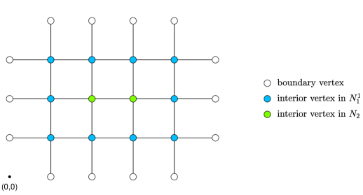
Figure 1. The graph $R_{4,3}$.

Lemma 2.2.

For any integers $m,n\geq 2$, the graph $R_{m,n}$ satisfies Assumption 1 and $\frac{|\partial G|(|\partial G|+1)}{2}\geq|G|$.

Proof.

For $1\leq l\leq\max\limits_{x\in G}d(x,\partial G)$, the set $N_{l}$ in $R_{m,n}$ is

$$N_{l}= \left\{l\vec{v}_{1}+(l+k)\vec{v}_{2}\mid 0\leq k\leq n-2l+1\right\}$$

$$\cup\left\{(m+1-l)\vec{v}_{1}+(l+k)\vec{v}_{2}\mid 0\leq k\leq n-2l+1\right\}$$

$$\cup\left\{(l+j)\vec{v}_{1}+l\vec{v}_{2}\mid 1\leq j\leq m-2l\right\}$$

$$\cup\left\{(l+j)\vec{v}_{1}+(n+1-l)\vec{v}_{2}\mid 1\leq j\leq m-2l\right\}.$$

The decomposition of $N_{l}$ is trivial as $N_{l}=N_{l}^{1}$. For each vertex respectively in the above four subsets of $N_{l}$, there exists a boundary vertex closest to it in $(\partial G)_{L},(\partial G)_{R},(\partial G)_{B}$ and $(\partial G)_{T}$ respectively.

To show the relation between the boundary and interior vertices, simply notice that $|\partial G|=2(m+n)$ and $|G|=mn$, thus $\frac{|\partial G|(|\partial G|+1)}{2}=(m+n)(2m+2n+1)\geq mn=|G|$. ∎

Example 2.3.

The graph $T_{m,n}$ with $m,n\geq 2$.

Take $\vec{v}_{1}=1+0{\rm i}$, $\vec{v}_{2}=\frac{1}{2}+\frac{\sqrt{3}}{2}{\rm i}$. Let $D_{0}\subset\mathbb{R}^{2}$ be the triangular domain with the set of 3 vertices $G_{0}:=\{\vec{v}_{1}+\vec{v}_{2},2\vec{v}_{1}+\vec{v}_{2},\vec{v}_{1}+2\vec{v}_{2}\}$. Define

$$\mathcal{D}_{m,n}:=\bigcup_{\begin{subarray}{c}0\leq j\leq m-2\\ 0\leq k\leq n-2\end{subarray}}(D_{0}+j\vec{v}_{1}+k\vec{v}_{2}),$$

where $j,k\in\mathbb{N}$. The set of interior vertices is

$$G:=\bigcup_{\begin{subarray}{c}0\leq j\leq m-2\\ 0\leq k\leq n-2\end{subarray}}(G_{0}+j\vec{v}_{1}+k\vec{v}_{2}),$$

The set of boundary vertices is $\partial G:=(\partial G)_{L}\cup(\partial G)_{R}\cup(\partial G)_{B}\cup(\partial G)_{T}$ with

$$(\partial G)_{L}:= \{k\vec{v}_{2}\mid 1\leq k\leq n\},\qquad(\partial G)_{R}:=\{(m+1)\vec{v}_{1}+k\vec{v}_{2}\mid 1\leq k\leq n\},$$

$$(\partial G)_{B}:= \{j\vec{v}_{1}\mid 1\leq j\leq m\},\qquad(\partial G)_{T}:=\{j\vec{v}_{1}+(n+1)\vec{v}_{2}\mid 1\leq j\leq m\}.$$

The definition of the edge set $\mathcal{E}$ is as follows: an edge is assigned to any pair of vertices in $\bar{G}$ of Euclidean distance $1$, where every boundary vertex in $\partial G$ connects to an interior vertex in $G$ whose coordinates differ by vectors $\vec{v}_{1}$ or $\vec{v}_{2}$. This graph is denoted by $T_{m,n}$, where $m,n$ indicate the number of interior vertices along the directions $\vec{v}_{1},\vec{v}_{2}$, respectively. As an example, $T_{6,4}$ is illustrated in Fig. 2.

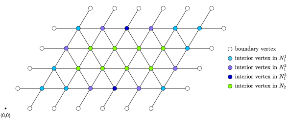
Figure 2. The graph $T_{6,4}$.

Lemma 2.4.

For any integers $m,n\geq 2$, the graph $T_{m,n}$ satisfies Assumption 1 and $\frac{|\partial G|(|\partial G|+1)}{2}\geq|G|$.

Proof.

For $1\leq l\leq\max\limits_{x\in G}d(x,\partial G)$, the set $N_{l}$ in $T_{m,n}$ is

$$N_{l}= \{l\vec{v}_{1}+(l+k)\vec{v}_{2}\mid 0\leq k\leq n-2l+1\}:=\{x_{0},x_{1},\cdots,x_{n-2l+1}\}$$

$$\cup\{(m-l+1)\vec{v}_{1}+(l+k)\vec{v}_{2}\mid 0\leq k\leq n-2l+1\}:=\{y_{0},y_{1},\cdots,y_{n-2l+1}\}$$

$$\cup\{(l+j)\vec{v}_{1}+l\vec{v}_{2}\mid 1\leq j\leq m-2l\}:=\{\gamma_{1},\cdots,\gamma_{m-2l}\}$$

$$\cup\{(l+j)\vec{v}_{1}+(n-l+1)\vec{v}_{2}\mid 1\leq j\leq m-2l\}:=\{\tau_{1},\cdots,\tau_{m-2l}\}.$$

For each vertex respectively in the above four subsets of $N_{l}$, there exists a boundary vertex closest to it in $(\partial G)_{L},(\partial G)_{R},(\partial G)_{B}$ and $(\partial G)_{T}$ respectively. The above $x_{r},y_{r},\gamma_{r},\tau_{r}$ when $r\in\mathbb{N}$ are numbers of the vertices in the sets.

Let integer $p\geq 2$. The decomposition of $N_{l}$ is

$$N_{l}^{1}= \{x_{0},x_{1},x_{n-2l+1},y_{0},y_{n-2l},y_{n-2l+1},\gamma_{1},\tau_{m-2l}\},$$

$$N_{l}^{p}= \{x_{p},x_{n-2l+2-p},y_{p-1},y_{n-2l-p+1}\mid p\leq n-2l+2-p\}$$

$$\cup\{\gamma_{p},\gamma_{m-2l+2-p},\tau_{p-1},\tau_{m-2l-p+1}\mid p\leq m-2l+2-p\},\quad p\geq 2.$$

To show the relation between the boundary and interior vertices, simply notice that $|\partial G|=2(m+n)$ and $|G|=mn$, thus $\frac{|\partial G|(|\partial G|+1)}{2}=(m+n)(2m+2n+1)\geq mn=|G|$. ∎

Example 2.5.

The graph $H_{m,n}$, where $m,n\geq 1$ and $m$ is odd.

Let $\omega=\frac{1}{2}+\frac{\sqrt{3}}{2}{\rm i}$, then $\omega^{6}=1$, where $6$ is the power of $\omega$. Take $\vec{v}_{1}=3\omega^{6}=3+0i$, $\vec{v}_{2}=0+\sqrt{3}{\rm i}$. Let $D_{0}\subset\mathbb{R}^{2}$ be the hexagon domain with the set of 6 vertices $G_{0}:=\{\omega^{0},\omega^{1},\omega^{2},\omega^{3},\omega^{4},\omega^{5}\}$. Define

$$\mathcal{D}_{m,n}:=\bigcup_{\begin{subarray}{c}0\leq j\leq\frac{m-1}{2}\\ 0\leq k\leq n-1\end{subarray}}(D_{0}+j\vec{v}_{1}+k\vec{v}_{2}),$$

where $j,k\in\mathbb{N}$. The set of interior vertices is

$$G:=\bigcup_{\begin{subarray}{c}0\leq j\leq\frac{m-1}{2}\\ 0\leq k\leq n-1\end{subarray}}(G_{0}+j\vec{v}_{1}+k\vec{v}_{2}),$$

The set of boundary vertices is $\partial G:=(\partial G)_{L}\cup(\partial G)_{R}\cup(\partial G)_{B}\cup(\partial G)_{T}$, where

$$(\partial G)_{L}:= \left\{k\vec{v}_{2}+2\omega^{3}\mid 0\leq k\leq n-1\right\},\quad(\partial G)_{R}:=\left\{k\vec{v}_{2}+\frac{3(m-1)}{2}+2\mid 0\leq k\leq n-1\right\},$$

$$(\partial G)_{B}:= \left\{j\vec{v}_{1}+2\omega^{4},j\vec{v}_{1}+2\omega^{4}+2\mid 0\leq j\leq\frac{m-1}{2}\right\},$$

$$(\partial G)_{T}:= \left\{j\vec{v}_{1}+(n-1)\vec{v}_{2}+2\omega^{2},j\vec{v}_{1}+(n-1)\vec{v}_{2}+2\omega^{2}+2\mid 0\leq j\leq\frac{m-1}{2}\right\}.$$

The edge set $\mathcal{E}$ is defined by assigning an edge to any pair of vertices in $\bar{G}$ that is of Euclidean distance $1$, where any two boundary vertices are not connected. This graph is denoted by $H_{m,n}$, where $m,n$ indicate the number of hexagons on the border along the directions $\vec{v}_{1},\vec{v}_{2}$, respectively. As an example, $H_{3,4}$ and its vertices decomposition are shown in Fig. 3.

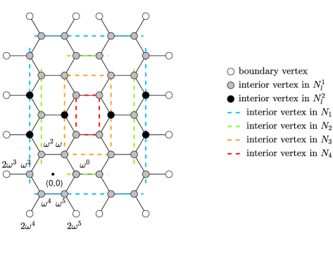
Figure 3. The graph $H_{3,4}$.

Lemma 2.6.

For any integers $m,n\geq 1$ and $m$ is odd, the graph $H_{m,n}$ satisfies Assumption 1 and $\frac{|\partial G|(|\partial G|+1)}{2}\geq|G|$.

Proof.

Let $1\leq l\leq\max\limits_{x\in G}d(x,\partial G)-1$.

For $l~{}mod~{}4=1$, the set $N_{l}$ in $H_{m,n}$ is

$$N_{l}= \left\{\frac{l-1}{4}\vec{v}_{1}+(\frac{l-1}{2}+k)\vec{v}_{2}+\omega^{3}\mid 0\leq k\leq n-l\right\}:=\{x_{0},x_{1},\cdots,x_{n-l}\}$$

$$\cup\left\{\frac{3(m-1)}{2}-\frac{l-1}{4}\vec{v}_{1}+(\frac{l-1}{2}+k)\vec{v}_{2}+\omega^{0}\mid 0\leq k\leq n-l\right\}:=\{y_{0},y_{1},\cdots,y_{n-l}\}$$

$$\cup\left\{(\frac{l-1}{4}+j)\vec{v}_{1}+\frac{l-1}{2}\vec{v}_{2}+\omega^{4},(\frac{l-1}{4}+j)\vec{v}_{1}+\frac{l-1}{2}\vec{v}_{2}+\omega^{5}\mid 0\leq j\leq\frac{m-l}{2}\right\}$$

$$\cup\left\{(\frac{l-1}{4}+j)\vec{v}_{1}+(n-\frac{l+1}{2})\vec{v}_{2}+\omega^{2},(\frac{l-1}{4}+j)\vec{v}_{1}+(n-\frac{l+1}{2})\vec{v}_{2}+\omega^{1}\mid 0\leq j\leq\frac{m-l}{2}\right\}.$$

For each vertex respectively in the above four subsets of $N_{l}$, there exists a boundary vertex closest to it in $(\partial G)_{L},(\partial G)_{R},(\partial G)_{B},(\partial G)_{T}$ respectively. The decomposition of $N_{l}$ is

$$N_{l}^{1}= N_{l}\setminus\{x_{1},x_{2},\cdots,x_{n-l-1},y_{1},y_{2},\cdots,y_{n-l-1}\},$$

$$N_{l}^{p+1}= \{x_{p},x_{n-l-p},y_{p},y_{n-l-p}\mid p\leq m-1-p\},\quad p\in\mathbb{N}_{+}.$$

For $l~{}mod~{}4=2$, the set $N_{l}$ in $H_{m,n}$ is

$$N_{l}= \left\{\frac{l-2}{4}\vec{v}_{1}+(\frac{l-2}{2}+k)\vec{v}_{2}+\omega^{2}\mid 0\leq k\leq n-l\right\}$$

$$\cup\left\{\frac{3(m-1)}{2}-\frac{l-2}{4}\vec{v}_{1}+(\frac{l-2}{2}+k)\vec{v}_{2}+\omega\mid 0\leq k\leq n-l\right\}$$

$$\cup\left\{(\frac{l-2}{4}+j)\vec{v}_{1}+\frac{l-2}{2}\vec{v}_{2}+\omega^{0},(\frac{l-2}{4}+j)\vec{v}_{1}+\frac{l-2}{2}\vec{v}_{2}+2\omega^{0}\mid 0\leq j\leq\frac{m-l-1}{2}\right\}$$

$$\cup\left\{(\frac{l-2}{4}+j)\vec{v}_{1}+(n-\frac{l}{2})\vec{v}_{2}+\omega^{0},(\frac{l-2}{4}+j)\vec{v}_{1}+(n-\frac{l}{2})\vec{v}_{2}+2\omega^{0}\mid 0\leq j\leq\frac{m-l-1}{2}\right\}.$$

For each vertex respectively in the above four subsets of $N_{l}$, there exists a boundary vertex closest to it in $(\partial G)_{L},(\partial G)_{R},(\partial G)_{B},(\partial G)_{T}$ respectively. The decomposition of $N_{l}$ is $N_{l}=N_{l}^{1}$.

For $l~{}mod~{}4=3$, the set $N_{l}$ in $H_{m,n}$ is

$$N_{l}= \left\{\frac{l-3}{4}\vec{v}_{1}+(\frac{l-3}{2}+k)\vec{v}_{2}+\omega\mid 1\leq k\leq n-l\right\}:=\{\gamma_{1},\cdots,\gamma_{n-l}\}$$

$$\cup\left\{\frac{3(m-1)}{2}-\frac{l-3}{4}\vec{v}_{1}+(\frac{l-3}{2}+k)\vec{v}_{2}+\omega^{2}\mid 1\leq k\leq n-l\right\}:=\{\tau_{1},\cdots,\tau_{n-l}\}$$

$$\cup\left\{(\frac{l-3}{4}+j)\vec{v}_{1}+\frac{l-3}{2}\vec{v}_{2}+\omega,(\frac{l-3}{4}+j)\vec{v}_{1}+\frac{l-3}{2}\vec{v}_{2}+\omega+2\mid 0\leq j\leq\frac{m-l}{2}\right\}$$

$$\cup\left\{(\frac{l-3}{4}+j)\vec{v}_{1}+(n-\frac{l-1}{2})\vec{v}_{2}+\omega^{5},(\frac{l-3}{4}+j)\vec{v}_{1}+(n-\frac{l-1}{2})\vec{v}_{2}+\omega^{5}+2\mid 0\leq j\leq\frac{m-l}{2}\right\}.$$

For each vertex respectively in the above four subsets of $N_{l}$, there exists a boundary vertex closest to it in $(\partial G)_{L},(\partial G)_{R},(\partial G)_{B},(\partial G)_{T}$, respectively. The decomposition of $N_{l}$ is

$$N_{l}^{1}= N_{l}\setminus\{\gamma_{1},\cdots,\gamma_{n-l},\tau_{1},\cdots,\tau_{n-l}\},$$

$$N_{l}^{p+1}= \{\gamma_{p},\gamma_{n-l-p},\tau_{p},\tau_{n-l-p}\mid p\leq m-1-p\},\quad p\in\mathbb{N}_{+}.$$

For $l~{}mod~{}4=0$, the set $N_{l}$ in $H_{m,n}$ is

$$N_{l}= \left\{\frac{l-4}{4}\vec{v}_{1}+(\frac{l-4}{2}+k)\vec{v}_{2}+2\omega\mid 1\leq k\leq n-l\right\}$$

$$\cup\left\{\frac{3(m-1)}{2}-\frac{l-4}{4}\vec{v}_{1}+(\frac{l-4}{2}+k)\vec{v}_{2}+2\omega^{2}\mid 1\leq k\leq n-l\right\}$$

$$\cup\left\{(\frac{l-4}{4}+j)\vec{v}_{1}+\frac{l-4}{2}\vec{v}_{2}+2\omega,(\frac{l-4}{4}+j)\vec{v}_{1}+\frac{l-4}{2}\vec{v}_{2}+2\omega+1\mid 0\leq j\leq\frac{m-l+1}{2}\right\}$$

$$\cup\left\{(\frac{l-4}{4}+j)\vec{v}_{1}+(n-\frac{l}{2}+1)\vec{v}_{2}+2\omega^{5},(\frac{l-4}{4}+j)\vec{v}_{1}+(n-\frac{l}{2}+1)\vec{v}_{2}+2\omega^{5}+1\right.$$

$$\left.\mid 0\leq j\leq\frac{m-l+1}{2}\right\}.$$

For each vertex respectively in the above four subsets of $N_{l}$, there exists a boundary vertex closest to it in $(\partial G)_{L},(\partial G)_{R},(\partial G)_{B},(\partial G)_{T}$ respectively. The decomposition of $N_{l}$ is $N_{l}=N_{l}^{1}$.

If $l=\max\limits_{x\in G}d(x,\partial G)$, take $N_{l}=N_{l}^{1}$.

To show the relation between the boundary and interior vertices, simply notice that $|\partial G|=2(m+n+1)$ and $|G|=(m+1)(2n+1)$, thus $\frac{|\partial G|(|\partial G|+1)}{2}=(m+n+1)(2m+2n+3)\geq(m+1)(2n+1)=|G|$. ∎

3. Proof of Theorem 1.5

We prove Theorem 1.5, which gives an explicit formula to represent the ND map in terms of the Neumann boundary spectral data.

The following Green’s formula is proved in [11, Lemma 2.1].

Lemma 3.1.

(Green’s formula). Let $u_{1},~{}u_{2}:~{}\bar{G}\rightarrow\mathbb{R}$ be two real-valued functions on $\bar{G}$. Then

$$(u_{1},\Delta_{G}u_{2})_{G}-(u_{2},\Delta_{G}u_{1})_{G}=(u_{2},\partial_{\nu}u_{1})_{\partial G}-(u_{1},\partial_{\nu}u_{2})_{\partial G}.$$

For each $j=1,2,\dots,|\partial G|$, the scalar orthogonal projection of the wave time solution $u^{f}(t)$ onto the Neumann eigenfunction $\phi_{j}$ is denoted by

$$a_{j}(t):=(u^{f}(t),\phi_{j})_{G}=\sum_{x\in G}\mu_{x}u^{f}(t,x)\phi_{j}(x),\quad t=0,1,2,\cdots.$$

These scalar orthogonal projections can be explicitly computed from the Neumann boundary spectral data as follows.

Lemma 3.2.

For $t=1,2,3,\dots$, we have

$$a_{j}(t)=c_{t}(f(1),\phi_{j})_{\partial G}+c_{t-1}(f(2),\phi_{j})_{\partial G}+\cdots+c_{2}(f(t-1),\phi_{j})_{\partial G}+c_{1}(f(t),\phi_{j})_{\partial G},$$ (3.1)

where the constants $c_{k}$ are defined recursively by $c_{1}=0$, $c_{2}=-1$, and $c_{k}=(2-\lambda_{j})c_{k-1}-c_{k-2}$ for $k\geq 3$.

Proof.

Apply $D_{tt}$ to $a_{j}$ to get

$$D_{tt}a_{j}(t) =(D_{tt}u^{f}(t),\phi_{j})_{G}$$

$$=(\Delta_{G}u^{f}(t),\phi_{j})_{G}$$

$$=(u^{f}(t),\Delta_{G}\phi_{j})_{G}-(f(t),\phi_{j})_{\partial G}$$

$$=-(u^{f}(t),\lambda_{j}\phi_{j})_{G}-(f(t),\phi_{j})_{\partial G}$$

$$=-\lambda_{j}a_{j}(t)-(f(t),\phi_{j})_{\partial G},$$

where the second equality follows from the wave equation, the third equality is derived from the Green’s formula in Lemma 3.1 with $\partial_{\nu}\phi_{j}=0$, and the final equality from the definition of $a_{j}(t)$. This is a finite difference equation for $a_{j}(t)$, which, using the definition of $D_{tt}$, can be defined by the inductive relation

$$a_{j}(t+1)=(2-\lambda_{j})a_{j}(t)-a_{j}(t-1)-(f(t),\phi_{j})_{\partial G}.$$

The initial conditions are given by

$$a_{j}(0)=(u^{f}(0),\phi_{j})_{G}=0,\quad a_{j}(1)=(u^{f}(1),\phi_{j})_{G}=0,$$

which are derived from the initial conditions of the function $u^{f}$. We now prove the validity of formula (3.1) by induction.

The base case $t=1$ is true since $c_{1}=0$. For the inductive step, suppose that the formula (3.1) has been proved for all positive integers less than or equal to $t$, then

$$a_{j}(t-1)= c_{t-1}(f(1),\phi_{j})_{\partial G}+\cdots+(\lambda_{j}-2)(f(t-3),\phi_{j})_{\partial G}-(f(t-2),\phi_{j})_{\partial G},$$

$$a_{j}(t)= c_{t}(f(1),\phi_{j})_{\partial G}+\cdots+(\lambda_{j}-2)(f(t-2),\phi_{j})_{\partial G}-(f(t-1),\phi_{j})_{\partial G}.$$

Insert these representations into the inductive relation to get

$$a_{j}(t+1) =(2-\lambda_{j})a_{j}(t)-a_{j}(t-1)-(f(t),\phi_{j})_{\partial G}$$

$$=((2-\lambda_{j})c_{t}-c_{t-1})(f(1),\phi_{j})_{\partial G}+\cdots+(-(2-\lambda_{j})^{2}+1)(f(t-2),\phi_{j})_{\partial G}$$

$$\quad-(2-\lambda_{j})(f(t-1),\phi_{j})_{\partial G}-(f(t),\phi_{j})_{\partial G}.$$

This completes the proof. ∎

Now, we prove Theorem 1.5.

Proof of Theorem 1.5.

As $\{\phi_{j}(x),x\in G\}^{|G|}_{j=1}$ forms an orthonormal basis of $l^{2}(G)$, we can write

$$u^{f}(t,x)=\sum^{|G|}_{j=1}(u^{f}(t),\phi_{j})_{G}\phi_{j}(x)=\sum^{|G|}_{j=1}a_{j}(t)\phi_{j}(x),\quad x\in G.$$

As each boundary vertex $z\in\partial G$ is connected to a unique interior vertex $x\in G$, using the definition of $\partial_{\nu}u(z)$ in (1.2), we get

$$f(t,z)=\partial_{\nu}u^{f}(t,z)=\frac{1}{\mu_{z}}w(x,z)(u^{f}(t,x)-u^{f}(t,z)).$$

Solving for the Dirichlet data of the wave solution from this relation, we can obtain

$$\Lambda_{\mu}f(t,z)=u^{f}(t,z)=u^{f}(t,x)-\frac{\mu_{z}f(t,z)}{w(x,z)}=\sum^{|G|}_{j=1}a_{j}(t)\phi_{j}(z)-\frac{\mu_{z}f(t,z)}{w(x,z)},\quad x\sim z,\qquad t\geq 1.$$

Theorem 1.5 is proved by substituting the expression for $a_{j}(t)$ into the summation given in equation (3.1). ∎

4. The reconstruction procedure

In this section, we introduce a discrete version of the boundary control method. Additionally, using this method, we will demonstrate the reconstruction procedure for the interior vertex weight.

4.1. Calculating Inner Products of Waves.

When $x$ serves as the spatial component of the function $u(t,x)$, we simply denote $u(t,x)$ as $u(t)$. For a function $u(t,x)$, we introduce the time reversal operator:

$$\mathscr{R}:l^{2}\left(\{1,\cdots,T-1\}\times{\partial G}\right)\longmapsto l^{2}(\{1,\cdots,T-1\}\times{\partial G}),$$

$$\mathscr{R}u(t):=u(T-t),\qquad t\in\{1,\cdots,T-1\}.$$

Similarly, we introduce another operator:

$$\mathscr{J}:l^{2}(\{0,1,\cdots,2T\}\times{\partial G})\longmapsto l^{2}(\{1,\cdots,T-1\}\times{\partial G}),$$

$$\mathscr{J}u(t):=\sum\limits_{j=0}^{T-t-1}u(t+1+2j),\qquad t\in\{1,\cdots,T-1\}.$$

Define $P_{T}:l^{2}(\{0,\cdots,2T\}\times{\partial G})\mapsto l^{2}(\{1,\cdots,T-1\}\times{\partial G})$ as the truncation operator, while the adjoint operator $P^{*}_{T}:l^{2}(\{1,\cdots,T-1\}\times{\partial G})\mapsto l^{2}(\{0,\cdots,2T\}\times{\partial G})$ is an extension operator. The values of $P^{*}_{T}$ on $\{0,T,T+1,\cdots,2T\}\times\partial G$ are extended by zero. Define the Dirichlet trace operator by $\tau_{D}u(t)=u(t)|_{\partial G}$ and the Neumann trace operator by $\tau_{N}u(t)=\partial_{\nu}u(t)|_{\partial G}$, respectively.

For functions $v_{1},v_{2}:\{1,\cdots,T-1\}\times\partial G\longrightarrow\mathbb{R}$, define the inner product on the boundary $l^{2}$-space $l^{2}(\{1,\cdots,T-1\}\times\partial G)$ as follows:

$$(v_{1},v_{2})_{\{1,\cdots,T-1\}\times\partial G}:=\sum^{T-1}_{t=1}(v_{1}(t),v_{2}(t))_{\partial G}=\sum\limits_{z\in\partial G}\mu_{z}\sum\limits_{t=1}^{T-1}v_{1}(t,z)v_{2}(t,z).$$

Here, for $z\in\partial G$, the values $\mu_{z}$ are known.

The following is a discrete counterpart of the generalized Blagovescenskii identity ([45]). The original Blagovescenskii identity is proved in ([13]).

Lemma 4.1.

Let $u^{f}$ be the solution of (1.5), and let $v\in l^{2}(\{0,\cdots,2T\}\times\bar{G})$ be the solution of the equation

$$D_{tt}v(t,x)-\Delta_{G}v(t,x)=0,\quad(t,x)\in\{1,2,\cdots,2T-1\}\times G,$$

then

$$(u^{f}(T),v(T))_{G}=(P_{T}(\Lambda_{\mu}f),\mathscr{J}\tau_{N}v)_{\{1,\cdots,T-1\}\times{\partial G}}-(P_{T}f,\mathscr{J}\tau_{D}v)_{\{1,\cdots,T-1\}\times\partial G}.$$

Proof.

Set

$$I(t,s):=(u^{f}(t),v(s))_{G},\quad t,s\in\mathbb{N},~{}t,s\geq 0.$$

Using equation (1.5) and the Green’s formula, we get

$$(D_{tt}-D_{ss})I(t,s)= (D_{tt}u^{f}(t),v(s))_{G}-(u^{f}(t),D_{ss}v(s))_{G}$$

$$= (\Delta_{G}u^{f}(t),v(s))_{G}-(u^{f}(t),\Delta_{G}v(s))_{G}$$

$$= (u^{f}(t),\partial_{\nu}v(s))_{\partial G}-(v(s),\partial_{\nu}u^{f}(t))_{\partial G}$$

$$= (\Lambda_{\mu}f(t),\tau_{N}v(s))_{\partial G}-(\tau_{D}v(s),f(t))_{\partial G},\quad s,t\geq 1.$$

Let us denote the right hand side by $F(t,s)$, i.e.,

$$F(t,s):=(\Lambda_{\mu}f(t),\tau_{N}v(s))_{\partial G}-(\tau_{D}v(s),f(t))_{\partial G}.$$

Using the definition of $D_{tt}$ and $D_{ss}$, the relation can be written as

$$I(t+1,s)=-I(t-1,s)+I(t,s+1)+I(t,s-1)+F(t,s),\quad t,s\geq 1$$ (4.1)

On the other hand, the initial conditions for $u^{f}$ are $u^{f}(0,x)=0$ for $x\in\bar{G}$ and $D_{t}u^{f}(0,x)=0$ for $x\in G$. Hence,

$$I(0,s)= (u^{f}(0),v(s))_{G}=0,\quad s\in\{0,1,\cdots,2T\},$$ (4.2)

$$I(1,s)= D_{t}I(0,s)+I(0,s)=(D_{t}u^{f}(0),v(s))_{G}+I(0,s)=0,\quad s\in\{0,1,\cdots,2T\}.$$

Consequently, we obtain a recursive relationship for $I(t,s)$ with initial conditions. The solution to this recursive relationship is given by

$$I(t,s)=\sum\limits_{i=1}^{t-1}\sum\limits_{j=0}^{t-i-1}F(i,s-t+i+1+2j),\qquad t\geq 2,\quad s\geq 1.$$ (4.3)

This solution can be proved by induction. Indeed, when $t=2$, we have from (4.1) and (4.2) that

$$I(2,s)=-I(0,s)+I(1,s+1)+I(1,s-1)+F(1,s)=F(1,s),$$

which agrees with the solution formula (4.3). This establishes the base case.

For the inductive step, suppose the solution formula (4.3) holds for all $t\leq k$ for some positive integers $k\geq 2$. Considering the case $t=k+1$ and using the recursive relation, we can get

$$I(k+1,s) =-I(k-1,s)+I(k,s+1)+I(k,s-1)+F(k,s)$$

$$=-\sum\limits_{i=1}^{k-2}\sum\limits_{j=0}^{k-i-2}F(i,s-k+i+2+2j)+\sum\limits_{i=1}^{k-1}\sum\limits_{j=0}^{k-i-1}F(i,s-k+i+2+2j)$$

$$+\sum\limits_{i=1}^{k-1}\sum\limits_{j=0}^{k-i-1}F(i,s-k+i+2j)+F(k,s)$$

$$:= -I_{1}+I_{2}+I_{3}+F(k,s).$$

Notice that

$$I_{2} =I_{1}+\sum^{k-2}_{i=1}F(i,s-k+i+2+2j)|_{j=k-i-1}+F(i,s-k+i+2+2j)|_{i=k-1,j=0}$$

$$=I_{1}+\sum^{k-2}_{i=1}F(i,s+k-i)+F(k-1,s+1)$$

$$=I_{1}+\sum^{k-1}_{i=1}F(i,s+k-i),$$

hence,

$$I(k+1,s) =-I_{1}+I_{2}+I_{3}+F(k,s)$$

$$=I_{3}+\sum^{k-1}_{i=1}F(i,s+k-i)+F(k,s)$$

$$=\sum\limits_{i=1}^{k-1}\sum\limits_{j=0}^{k-i-1}F(i,s-k+i+2j)+\sum^{k-1}_{i=1}F(i,s+k-i)+F(k,s)$$

$$=\sum\limits_{i=1}^{k-1}\left(\sum\limits_{j=0}^{k-i-1}F(i,s-k+i+2j)+F(i,s-k+i+2j)|_{j=k-i}\right)+F(k,s)$$

$$=\sum\limits_{i=1}^{k-1}\left(\sum\limits_{j=0}^{k-i}F(i,s-k+i+2j)\right)+F(i,s-k+i+2j)|_{i=k,j=0}$$

$$=\sum\limits_{i=1}^{k}\sum\limits_{j=0}^{k-i}F(i,s-k+i+2j),$$

which agrees with the solution formula (4.3) with $t=k+1$. This completes the induction.

Finally, by substituting $t=s=T$ into (4.3), we obtain the following expression

$$\begin{split}(u^{f}(T),v(T))_{G}=&I(T,T)\\ =&\sum\limits_{i=1}^{T-1}\sum\limits_{j=0}^{T-i-1}F(i,i+1+2j)\\ =&\sum\limits_{i=1}^{T-1}\sum\limits_{j=0}^{T-i-1}\left[(\Lambda_{\mu}f(i),\tau_{N}v(i+1+2j))_{\partial G}-(\tau_{D}v(i+1+2j),f(i))_{\partial G}\right]\\ =&\sum\limits_{i=1}^{T-1}\left[(\Lambda_{\mu}f(i),\sum\limits_{j=0}^{T-i-1}\tau_{N}v(i+1+2j))_{\partial G}-(f(i),\sum\limits_{j=0}^{T-i-1}\tau_{D}v(i+1+2j))_{\partial G}\right]\\ =&\sum_{i=1}^{T-1}\left[(\Lambda_{\mu}f(i),\mathscr{J}\tau_{N}v(i))_{\partial G}-(f(i),\mathscr{J}\tau_{D}v(i))_{\partial G}\right]\\ =&(P_{T}(\Lambda_{\mu}f),\mathscr{J}\tau_{N}v)_{\{1,\cdots,T-1\}\times\partial G}-(P_{T}f,\mathscr{J}\tau_{D}v)_{\{1,\cdots,T-1\}\times\partial G}.\end{split}$$

∎

Lemma 4.1 shows that $(u^{f}(T),v(T))_{G}$ can be expressed by the ND map $\Lambda_{\mu}$. Next, we approximate the wave on interior vertices at time $T$.

Define a linear operator $W:l^{2}(\{1,\cdots,T-1\}\times\partial G)\longmapsto l^{2}(G)$ which is $h\longmapsto u^{P^{*}_{T}h}(T,x),~{}x\in G$. It maps the Neumann boundary value to the solution of equation (1.5) at time $t=T$ and $x\in G$. Denote its adjoint operator by $W^{*}$.

4.2. Calculating $W^{*}W$

Let $\Lambda_{\mu,T}$ be the restricted ND map, for $h\in l^{2}({\{1,\cdots,T-1\}\times\partial G})$,

$$\Lambda_{\mu,T}h:=P_{T}(\Lambda_{\mu}P_{T}^{*}h)=u^{P_{T}^{*}h}|_{\{1,\cdots,T-1\}\times\partial G}.$$

The Blagoveščenskiĭ’s identity was proposed in [13]. Let us give the following discrete version.

Proposition 4.2.

Let $h_{1},h_{2}\in l^{2}(\{1,2,\cdots,T\}\times\partial G)$, and $u^{P_{T}^{*}h_{1}}$, $u^{P_{T}^{*}h_{2}}$ be the solution of (1.5) with Neumann boundary values $P_{T}^{*}{h_{1}},P_{T}^{*}{h_{2}}\in l^{2}(\{0,1,\cdots,2T\}\times\partial G)$ respectively. Then, we can obtain

$$(u^{P_{T}^{*}h_{1}}(T),u^{P_{T}^{*}h_{2}}(T))_{G} =(Wh_{1},Wh_{2})_{G}=(h_{1},W^{*}Wh_{2})_{\{1,2,\cdots,T-1\}\times\partial G}$$

$$=(h_{1},(\mathscr{R}\Lambda_{\mu,T}\mathscr{R}\mathscr{J}P^{*}_{T}-\mathscr{J}\Lambda_{\mu}P_{T}^{*})h_{2})_{\{1,2,\cdots,T-1\}\times\partial G}.$$

Proof.

As $\tau_{D}u^{P_{T}^{*}h_{2}}=\Lambda_{\mu}P_{T}^{*}h_{2}$, $\tau_{N}u^{P_{T}^{*}h_{2}}=P_{T}^{*}h_{2}$, by Lemma 4.1 we have

$$(u^{P_{T}^{*}h_{1}}(T),u^{P_{T}^{*}h_{2}}(T))_{G} =(P_{T}(\Lambda_{\mu}P_{T}^{*}h_{1}),\mathscr{J}P^{*}_{T}h_{2})_{\{1,2,\cdots,T-1\}\times\partial G}-(h_{1},\mathscr{J}\Lambda_{\mu}P^{*}_{T}h_{2})_{\{1,2,\cdots,T-1\}\times\partial G}$$

$$=(\Lambda_{\mu,T}h_{1},\mathscr{J}P^{*}_{T}h_{2})_{\{1,2,\cdots,T-1\}\times\partial G}-(h_{1},\mathscr{J}\Lambda_{\mu}P^{*}_{T}h_{2})_{\{1,2,\cdots,T-1\}\times\partial G}$$

$$=(h_{1},\Lambda_{\mu,T}^{*}\mathscr{J}P^{*}_{T}h_{2})_{\{1,2,\cdots,T-1\}\times\partial G}-(h_{1},\mathscr{J}\Lambda_{\mu}P^{*}_{T}h_{2})_{\{1,2,\cdots,T-1\}\times\partial G}.$$

The adjoint is $\Lambda_{\mu,T}^{*}=\mathscr{R}\Lambda_{\mu,T}\mathscr{R}$ ( see Appendix B for the calculation). Thus,

$$(u^{P_{T}^{*}h_{1}}(T),u^{P_{T}^{*}h_{2}}(T))_{G}=(h_{1},(\mathscr{R}\Lambda_{\mu,T}\mathscr{R}\mathscr{J}P_{T}^{*}-\mathscr{J}\Lambda_{\mu}P_{T}^{*})h_{2})_{\{1,2,\cdots,T-1\}\times\partial G}.$$

On the other hand, the definition of the operator $W$ implies

$$(u^{P_{T}^{*}h_{1}}(T),u^{P_{T}^{*}h_{2}}(T))_{G}=(Wh_{1},Wh_{2})_{G}=(h_{1},W^{*}Wh_{2})_{\{1,2,\cdots,T-1\}\times\partial G}.$$

Since $h_{1},h_{2}$ are arbitrary, we can conclude that

$$W^{*}W=\mathscr{R}\Lambda_{\mu,T}\mathscr{R}\mathscr{J}P_{T}^{*}-\mathscr{J}\Lambda_{\mu}P_{T}^{*}.$$ (4.4)

∎

The next proposition presents an explicit formula for computing the action of the operator $W^{*}$ on any harmonic function $\varphi$.

Proposition 4.3.

For $h\in l^{2}(\{1,2,\cdots,T\}\times\partial G)$, let $u^{P_{T}^{*}h}$ be the solution of equation  (1.5) with the Neumann boundary value $P_{T}^{*}h\in l^{2}(\{0,1,\cdots,2T\}\times\partial G)$. If $\varphi(x)$ is an arbitrary harmonic function, then

$$(u^{P_{T}^{*}h}(T),\varphi)_{G}=(h,(\mathscr{R}\Lambda_{\mu,T}\mathscr{R}\mathscr{J}\tau_{N}-\mathscr{J}\tau_{D})\varphi)_{\{1,2,\cdots,T-1\}\times\partial G}.$$

Therefore,

$$W^{*}\varphi=(\mathscr{R}\Lambda_{\mu,T}\mathscr{R}\mathscr{J}\tau_{N}-\mathscr{J}\tau_{D})\varphi.$$ (4.5)

Proof.

We take $f=P_{T}^{*}h$, $v=\varphi$ in Lemma 4.1 and use the fact that $\Lambda_{\mu,T}^{*}=\mathscr{R}\Lambda_{\mu,T}\mathscr{R}$ (see Appendix B) to get

$$(u^{P_{T}^{*}h}(T),\varphi)_{G} =(P_{T}(\Lambda_{\mu}P_{T}^{*}h),\mathscr{J}\tau_{N}\varphi)_{\{1,2,\cdots,T-1\}\times\partial G}-(h,\mathscr{J}\tau_{D}\varphi)_{\{1,2,\cdots,T-1\}\times\partial G}$$

$$=(\Lambda_{\mu,T}h,\mathscr{J}\tau_{N}\varphi)_{\{1,2,\cdots,T-1\}\times\partial G}-(h,\mathscr{J}\tau_{D}\varphi)_{\{1,2,\cdots,T-1\}\times\partial G}$$

$$=(h,\Lambda_{\mu,T}^{*}\mathscr{J}\tau_{N}\varphi)_{\{1,2,\cdots,T-1\}\times\partial G}-(h,\mathscr{J}\tau_{D}\varphi)_{\{1,2,\cdots,T-1\}\times\partial G}$$

$$=(h,(\mathscr{R}\Lambda_{\mu,T}\mathscr{R}\mathscr{J}\tau_{N}-\mathscr{J}\tau_{D})\varphi)_{\{1,2,\cdots,T-1\}\times\partial G}.$$

On the other hand, the definition of $W$ gives

$$(u^{P_{T}^{*}h}(T),\varphi)_{G}=(Wh,\varphi)_{G}=(h,W^{*}\varphi)_{\{1,2,\cdots,T-1\}\times\partial G}.$$

As $h$ is arbitrary, we conclude that the action of $W^{*}$ on a harmonic function $\varphi(x)$ is

$$W^{*}\varphi=(\mathscr{R}\Lambda_{\mu,T}\mathscr{R}\mathscr{J}\tau_{N}-\mathscr{J}\tau_{D})\varphi.$$

∎

4.3. Solving the Boundary Control Equation

We aim to determine the existence of a function $h\in l^{2}(\{1,\cdots,T-1\}\times\partial G)$ such that $Wh=u^{P_{T}^{*}h}(T,x)$ holds for $x\in G$. In fact, we need to verify that $W$ is surjective.

Proposition 4.4.

Suppose the graph satisfies Assumption 1. If $T\geq\max\limits_{x\in G}d(x,\partial G)$, then $W$ is surjective.

Proof.

Note that $W$ is a linear operator between finite dimensional vector spaces. It remains to show that its adjoint operator $W^{*}$ is injective.

Given any $g\in l^{2}(G)$, we have (see Appendix B for the derivation)

$$W^{*}g=v(t,z)$$

with $(t,z)\in\{{1,2,\cdots,T-1\}\times\partial G}$, where $v$ satisfies

$$\begin{cases}D_{tt}v(t,x)-\Delta_{G}v(t,x)=0,&(t,x)\in\{1,2,\cdots,T-1\}\times G,\\ v(T,x)=0,&x\in\bar{G},\\ D_{t}v(T-1,x)=g(x),&x\in G,\\ \partial_{\nu}v(t,z)=0,&(t,z)\in\{0,1,\cdots,T\}\times\partial G.\end{cases}$$ (4.6)

Introduce $V(t):=v(T-t)$. Then $V$ solves

$$\begin{cases}D_{tt}V(t,x)-\Delta_{G}V(t,x)=0,&(t,x)\in\{1,2,\cdots,T-1\}\times G,\\ V(0,x)=0,&x\in\bar{G},\\ D_{t}V(0,x)=-g(x),&x\in G,\\ \partial_{\nu}V(t,z)=0,&(t,z)\in\{0,1,\cdots,T\}\times\partial G.\end{cases}$$

Let $V_{odd}(t,x)$ be the odd extension of $V(t,x)$ with respect to $t$, that is

$$V_{odd}(t)=\begin{cases}-V(t,x),&t\in\{-T,-T+1,\cdots,-1\},\\ V(t,x),&t\in\{0,1,\cdots,T\}.\end{cases}$$

By construction, $V_{odd}(t,x)$ clearly satisfies the wave equation for $t>0$ and $t<0$. For $t=0$, we use $V_{odd}(0,x)=0$ to get

$$D_{tt}V_{odd}(0,x)-\Delta_{G}V_{odd}(0,x)= V_{odd}(1,x)-2V_{odd}(0,x)+V_{odd}(-1,x)-\Delta_{G}V_{odd}(0,x)$$

$$= V(1,x)-V(1,x)$$

$$= 0.$$

Therefore, $V_{odd}(t,x)$ satisfies

$$\begin{cases}D_{tt}V_{odd}(t,x)-\Delta_{G}V_{odd}(t,x)=0,&(t,x)\in\{-T+1,\cdots,T-1\}\times G,\\ V_{odd}(0,x)=0,&x\in\bar{G},\\ D_{t}V_{odd}(0,x)=-g(x),&x\in G,\\ \partial_{\nu}V_{odd}(t,z)=0,&(t,z)\in\{-T,\cdots,T\}\times\partial G.\end{cases}$$

If $W^{*}g(x)=0$ for $x\in G$, then $V_{odd}(t,z)=0$ for $(t,z)\in\{-T,\cdots,T\}\times\partial G$. By the unique continuation property in Theorem 1.4, we have

$$D_{t}V(0,x)=D_{t}V_{odd}(0,x)=-g(x)=0$$

for every $x\in G$ when $T\geq\max\limits_{x\in G}d(x,\partial G)$. Therefore, $W^{*}$ is injective, which implies that $W$ is surjective. ∎

Proposition 4.5.

Suppose the graph satisfies Assumption 1 and $T\geq\max\limits_{x\in G}d(x,\partial G)$. For any harmonic function $\psi$, the boundary Neumann data given by

$$h_{0}=(W^{*}W)^{\dagger}W^{*}\psi$$ (4.7)

satisfies $u^{P_{T}^{*}h_{0}}(T,x)=\psi(x)$ for $x\in G$. Here ${\cdot}^{\dagger}$ denotes the pseudo-inverse.

Proof.

If $T\geq\max\limits_{x\in G}d(x,\partial G)$, we know that $W:l^{2}({\{1,\cdots,T-1\}\times\partial G})\longmapsto l^{2}(G)$ is surjective by Proposition 4.4. Hence, the equation $u^{P_{T}^{*}h}(T)=Wh=\psi$ admits solutions. It remains to prove the explicit formula (4.7).

Define a quadratic functional $\mathcal{F}$ by

$$\mathcal{F}(h):=\|u^{P_{T}^{*}h}(T)-\psi\|_{G}^{2} =\|Wh-\psi\|_{G}^{2}$$

$$=(Wh,Wh)_{G}-2(Wh,\psi)_{G}+\|\psi\|_{G}^{2}$$

$$=(h,W^{*}Wh)_{\{1,2,\cdots,T-1\}\times\partial G}-2(h,W^{*}\psi)_{\{1,2,\cdots,T-1\}\times\partial G}+\|\psi\|_{G}^{2}.$$

The gradient and Hessian matrix of $\mathcal{F}$ are

$$\mathcal{F}^{\prime}(h)=2W^{*}Wh-2W^{*}\psi,\quad\mathcal{F}^{\prime\prime}(h)=2W^{*}W.$$

Since the Hessian matrix is positive semi-definite, the function $\mathcal{F}$ is convex. Consequently, a local minimum of $\mathcal{F}$ is also a global minimum. To find a local minimum, we set $\mathcal{F}^{\prime}(h)=0$ to obtain the normal equation

$$W^{*}Wh_{0}=W^{*}\psi.$$

This is an under-determined linear system, and its minimum norm least squares solution is given by (4.7). ∎

Note that $W^{*}W$, and $W^{*}\psi$ can be computed explicitly from the ND map using Proposition 4.2 and Proposition 4.3. Therefore, the formula (4.7) provides an explicit construction of a boundary control.

4.4. Constructing $\mu$

Define

$$M={\rm span}\{\varphi\psi|_{G}:\varphi,\psi\in l^{2}(\bar{G}),\Delta_{G}\varphi(x)=\Delta_{G}\psi(x)=0,\ x\in G\},$$ (4.8)

that is, $M$ is the span of all the products of harmonic function on $G$. Note that as $\mu_{x}>0$ for each $x\in G$, the concept of harmonic functions is independent of the weight $\mu$, and so is $M$.

Let us give the proof of Theorem 1.6.

Proof.

Given two harmonic functions $\psi(x)$ and $\varphi(x)$ on the graph, we can find a boundary control $h_{0}$ such that $u^{P_{T}^{*}h_{0}}(T)=\psi$ by applying Proposition 4.5. Consequently, the following identity holds:

$$\sum\limits_{x\in G}\mu_{x}\psi(x)\varphi(x)=(\psi,\varphi)_{G}=(u^{P_{T}^{*}h_{0}}(T),\varphi)_{G}=(Wh_{0},\varphi)_{G}=(h_{0},W^{*}\varphi)_{\{1,2,\cdots,T-1\}\times\partial G}.$$ (4.9)

The right-hand side can be explicitly calculated using Proposition 4.3. The left-hand side represents the inner product of $\mu$ with the product $\psi\varphi$. By varying the harmonic functions $\psi,\varphi$, we can compute the orthogonal projection of $\mu|_{G}$ onto the space $M$. ∎

5. Uniqueness and Reconstruction

The proof only reconstructs the orthogonal projection of $\mu\in l^{2}(G)$ on the subspace $M\subset l^{2}(G)$ but not $\mu$ itself. General speaking, $M\neq l^{2}(G)$, see the discussion below. This is in contrast to the well-known fact that the products of (continuum) harmonic functions on a bounded open set $\Omega\subset\mathbb{R}^{n}$ $(n\geq 2)$ is dense in $L^{2}(\Omega)$ [16]. However, we can identify some sufficient conditions so that $M=l^{2}(G)$ for a generic class of edge weight functions.

Let us index all the vertices $x\in\bar{G}$ so that the interior vertices are indexed by $x_{1},\dots,x_{|G|}$ and the boundary vertices by $x_{|G|+1},\dots,x_{|\bar{G}|}$. Let $\varphi^{(j)}$ solve the boundary value problem

$$\Delta_{G}\varphi^{(j)}(x)=0\text{ for }x\in G,\qquad\varphi^{(j)}|_{\partial G}=\delta^{(j)}$$ (5.1)

where $\delta^{(j)}$ is a function on $\partial G$ such that

$$\delta^{(j)}=\begin{cases}1\quad\text{on}~{}x_{|G|+j},\\ 0\quad\text{on}~{}\partial G\backslash\{x_{|G|+j}\}.\end{cases}$$

This boundary value problem admits a unique solution, see Lemma C.1. Denote the space

$$H:={\rm span}\{\varphi^{(j)}\in l^{2}(\bar{G}):j=1,2,\dots,|\partial G|\}.$$

Lemma 5.1.

H is the space of harmonic functions on $\bar{G}$.

Proof.

It is clear that any function in $H$, as a linear combination of harmonic functions, is harmonic. Conversely, suppose $\varphi\in l^{2}(\bar{G})$ is an arbitrary harmonic function. Define

$$\tilde{\varphi}:=\sum^{|\partial G|}_{j=1}\varphi(x_{|G|+j})\varphi^{(j)}\quad\in H.$$

Then $\tilde{\varphi}$ is a harmonic function and $\tilde{\varphi}|_{\partial G}=\sum^{|\partial G|}_{j=1}\varphi(x_{|G|+j})\delta^{(j)}=\varphi|_{\partial G}$. We conclude $\varphi=\tilde{\varphi}$ by Lemma C.1, hence $\varphi\in H$. ∎

Using the indices, we can vectorize functions on $\bar{G}$ as follows: A function $u\in l^{2}(\bar{G})$ can be identified with a vector $\vec{u}=(u(x_{1}),\dots,u(x_{|\bar{G}|}))^{T}\in\mathbb{R}^{|\bar{G}|}$ via

$$l^{2}(\bar{G})\ni u\leftrightarrow\vec{u}:=\left(\begin{aligned} \vec{u}_{G}\\ \vec{u}_{\partial G}\\ \end{aligned}\right)\in\mathbb{R}^{|G|}\times\mathbb{R}^{|\partial G|}.$$ (5.2)

The vectorized space of harmonic functions is

$$\vec{H}:={\rm span}\{\vec{\varphi}^{(j)}\in\mathbb{R}^{|\bar{G}|}:j=1,2,\dots,|\partial G|\}.$$

The vectorized space of products of harmonic functions on $G$ is

$$\vec{M}:={\rm span}\left\{\vec{\varphi}^{(j)}_{G}\odot\vec{\varphi}^{(k)}_{G}\in\mathbb{R}^{|G|}:\;j,k=1,2,\dots,|\partial G|\right\}$$ (5.3)

where $\odot$ is the Hadamard product between two vectors.

Using the indices, the graph Laplacian $\Delta_{G}:\bar{G}\rightarrow G$ is identified with a block matrix

$$[\Delta_{G}]=([\Delta_{G,G}],[\Delta_{G,\partial G}])\;\in\mathbb{R}^{|G|\times|\bar{G}|},$$

where $[\Delta_{G,G}]\in\mathbb{R}^{|G|\times|G|},\;[\Delta_{G,\partial G}]\in\mathbb{R}^{|G|\times|\partial G|}.$ Then $\vec{\varphi}\in\mathbb{R}^{|\bar{G}|}$ is a vectorized harmonic function if and only if $[\Delta_{G}]\vec{\varphi}=0$. The discussion along with the rank-nullity relation leads to the following conclusion:

Lemma 5.2.

$$\vec{H}=\ker[\Delta_{G}]\quad\text{ and }\quad\dim\vec{H}+{\rm rank}[\Delta_{G}]=|\bar{G}|.$$

The discussion in the rest of this section adapts ideas from [14]. Let us construct a matrix $\mathbf{H}$ using $\vec{\varphi}^{(j)}_{G}\odot\vec{\varphi}^{(k)}_{G}$ as columns, where $j\leq k$, and $j,k=1,\dots,|\partial G|$. It is evident that $\mathbf{H}\in\mathbb{R}^{|G|\times\frac{|\partial G|(|\partial G|+1)}{2}}$ and the range of $\mathbf{H}$ is $\vec{M}$. Moreover, the following three statements are equivalent:

1. $M=l^{2}(G)$.

2. $\vec{M}=\mathbb{R}^{|G|}$.

3. ${\rm rank}(\mathbf{H})=|G|$.

Remark 5.3.

Since the rank of a matrix cannot exceed the number of columns, a necessary condition for $rank(\mathbf{H})=|G|$ is that $\frac{|\partial G|(|\partial G|+1)}{2}\geq|G|$. This condition requires the graph to have sufficient boundary vertices relative to the interior vertices.

Note that the entries in $\mathbf{H}$ depend on the edge weight function $w_{x,y}\in\mathbb{R}_{+}^{|\mathcal{E}|}$, since the definition of $\Delta_{G}$ involves $w_{x,y}$. We have the following alternatives for ${\rm rank}(\mathbf{H})$ with respect to $w_{x,y}$.

Proposition 5.4.

If the graph satisfies $\frac{|\partial G|(|\partial G|+1)}{2}\geq|G|$, then exactly one of the following cases occurs:

1. there is no edge weight function $w_{x,y}\in\mathbb{R}_{+}^{|\mathcal{E}|}$ such that ${\rm rank}(\mathbf{H})=|G|$;

2. ${\rm rank}(\mathbf{H})=|G|$ for all edge weight functions $w_{x,y}\in\mathbb{R}_{+}^{|\mathcal{E}|}$ except for a set of measure zero.

Proof.

Let $\beta$ be an arbitrary selection of $|G|$ columns from $\mathbf{H}$. Observe that

$${\rm rank}(\mathbf{H})=|G|\quad\text{ if and only if }\quad\exists~{}\beta\text{ such that }\det(\mathbf{H}_{:,\beta})\neq 0,$$

or equivalently,

$${\rm rank}(\mathbf{H})<|G|\quad\text{ if and only if }\quad\det(\mathbf{H}_{:,\beta})=0,\ \ \forall\beta.$$

We will use the fact that for a fixed $\beta$, $\det(\mathbf{H}_{:,\beta})$ is a real analytic function of $w_{x,y}$, see Lemma C.2.

If $\det(\mathbf{H}_{:,\beta})$ is the zero function for all $\beta$, that is, if $\det(\mathbf{H}_{:,\beta})\equiv 0$ regardless of $w_{x,y}$ for all $\beta$, then there is no edge weight function such that ${\rm rank}(\mathbf{H})=|G|$ holds, accounting for Case (1). On the other hand, if there exists $\beta$ such that $\det(\mathbf{H}_{:,\beta})$ is not the zero function, that is $\det(\mathbf{H}_{:,\beta})\not\equiv 0$, then it is a non-trivial real analytic function of $w_{x,y}$, hence the zeros

$$S_{\beta}:=\{w_{x,y}\in\mathbb{R}_{+}^{|\mathcal{E}|}:\det(\mathbf{H}_{:,\beta})=0\}$$

form a set of measure zero [37]. The collection of edge weight functions that ensure ${\rm rank}(\mathbf{H})<|G|$ is

$$\{w_{x,y}\in\mathbb{R}_{+}^{|\mathcal{E}|}:{\rm rank}(\mathbf{H})<|G|\}$$

$$= \{w_{x,y}\in\mathbb{R}_{+}^{|\mathcal{E}|}:\det(\mathbf{H}_{:,\beta})=0,\;\forall\beta\}$$

$$= \bigcap_{\beta}S_{\beta}.$$

This is a finite intersection of sets of measure zero, hence is also of measure zero.

∎

We remark that Case (1) in Proposition 5.4 can indeed occur. Here is an example.

Example 5.5.

For the graph in Fig. 4, $|\partial G|=|G|=2$. It is easy to see that the graph satisfies Assumption 1 and $\frac{|\partial G|(|\partial G|+1)}{2}=3>|G|=2$. For $x_{1},x_{2}\in G$ and $z_{1},z_{2}\in\partial G$, matrix $\mathbf{H}_{:,i+(j-1)|\partial G|}=[{\Delta_{G,G}^{-1}}\Delta_{G,\partial G}]_{:,i}\odot[{\Delta_{G,G}^{-1}}\Delta_{G,\partial G}]_{:,j}$, where $1\leq i,j\leq|\partial G|$ and $\mathbf{H}$ is independent on vertex weight. $\mathbf{H}$ is obviously a $|G|\times|\partial G|^{2}$ matrix. In this case,

$$\begin{split}\mathbf{H}=\frac{1}{(w_{x_{1},z_{1}}+w_{x_{1},z_{2}})^{2}}\begin{pmatrix}w_{x_{1},z_{1}}^{2}&w_{x_{1},z_{1}}w_{x_{1},z_{2}}&w_{x_{1},z_{1}}w_{x_{1},z_{2}}&w_{x_{1},z_{2}}^{2}\\ w_{x_{1},z_{1}}^{2}&w_{x_{1},z_{1}}w_{x_{1},z_{2}}&w_{x_{1},z_{1}}w_{x_{1},z_{2}}&w_{x_{1},z_{2}}^{2}\end{pmatrix},\end{split}$$

and ${\rm rank}(\mathbf{H})=1<|G|=2$.

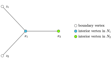
Figure 4. The interior vertex weight cannot be reconstructed by our method.

6. Reconstruction Algorithm

In this section, we implement the reconstruction procedure and validate it using numerical examples. Here, the reconstruction procedure is summarized in Algorithm 1.

0:  Time reversal operator $\mathscr{R}$, operator $\mathscr{J}$, truncation operator $P_{T}$, boundary vertex weight $\mu|_{\partial G}$ and the Neumann boundary spectral data $\{(\lambda_{j},\phi_{j}|_{\partial G})_{j=1}^{|G|}\}$.

1:  Calculate the ND map $\Lambda_{\mu}$ from the Neumann boundary spectral data by

$$\Lambda_{\mu}f(t,z)=u^{f}(t,z)=\sum^{|G|}_{j=1}\sum\limits_{k=1}^{t}c_{k}(f(t+1-k),\phi_{j})_{\partial G}\phi_{j}(z)-\frac{\mu_{z}f(t,z)}{w(x,z)},\quad x\sim z,$$

for $t\geq 1$, where $c_{1}=0,c_{2}=-1$, and $c_{k}=(2-\lambda_{j})c_{k-1}-c_{k-2}$ for integer $k\geq 3$ (see (1.6)).

2:  Calculate the operator $W^{*}W=\mathscr{R}\Lambda_{\mu,T}\mathscr{R}\mathscr{J}P_{T}^{*}-\mathscr{J}\Lambda_{\mu}P_{T}^{*}$ (see (4.4)).

3:  Calculate the operator $W^{*}$ operating on a harmonic function $\psi$ on a graph

$$W^{*}\varphi=(\mathscr{R}\Lambda_{\mu,T}\mathscr{R}\mathscr{J}\tau_{N}-\mathscr{J}\tau_{D})\varphi\quad\text{({\rm see } \eqref{Wstarformula})}.$$

4:  Solve $h_{0}$ from $W^{*}Wh_{0}=W^{*}\psi$, where $\psi$ is a harmonic function on the graph (see (4.7)).

5:  Construct the harmonic functions $\psi(x)$ and $\varphi(x)$ on the graph to reconstruct $\mu|_{G}$ from

$$(u^{P_{T}^{*}h_{0}}(T),\varphi)_{G}=(\psi,\varphi)_{G}=\sum\limits_{x\in G}\mu_{x}\psi(x)\varphi(x)=(h_{0},W^{*}\varphi)_{\{1,2,\cdots,T-1\}\times\partial G}\quad\text{ ({\rm see} \eqref{solvemu_xformula})}.$$

6:  return  $\mu|_{G}$.

6:  The interior vertex weight, $\mu|_{G}$;

Algorithm 1 Reconstruction Algorithm of the interior vertex weight.

To implement the algorithm, we will index the vertices so that functions on graphs can be identified with vectors, and linear operators on graphs can be identified with matrices. Recall that the vertices of $\bar{G}$ are ordered in the way that the interior vertices are indexed by $x_{1},\dots,x_{|G|}$ and the boundary vertices by $x_{|G|+1},\dots,x_{|\bar{G}|}$. For a spatial function $u\in l^{2}(\bar{G})$, it is vectorized as in (5.2). For a spatiotemporal function $f(t,x)$ with $t=0,1,2,\dots,T$ and $x\in\bar{G}$, we follow the lexicographical order to identify

$$f\leftrightarrow\vec{f}:=(f(0,\cdot),f(1,\cdot),\cdots,f(T,\cdot))^{*},$$

where $*$ denotes the adjoint, which is the transpose for a real vector. Using such an ordering, linear operators can be identified with matrices. For instance, the ND map $\Lambda_{\mu}$ is realized as an ND matrix via the following identification

$$\Lambda_{\mu}:l^{2}(\{0,1,\dots,2T\}\times\partial G)\rightarrow l^{2}(\{0,1,\dots,2T\}\times\partial G)\leftrightarrow[\Lambda_{\mu}]\in\mathbb{R}^{|\partial G|(2T+1)\times|\partial G|(2T+1)}$$

where we use the square parenthesis $[\cdot]$ to indicate matrix representations of linear operators.

The algorithm is implemented in the following steps.

Step 1: Assemble the Discrete Neumann-to-Dirichlet matrix. Given the Neumann boundary spectral data, the ND matrix can be readily calculated by following the formula presented in  (1.6). See Fig. 5 for an example of the ND matrix.

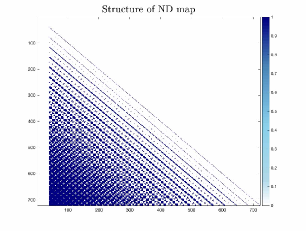
Figure 5. The structure of the ground-truth ND map $[\Lambda_{\mu}]$ for the graph $R_{m,n}$ when $m=10,n=9,|\partial G|=38,T=9$. Blank space represents zero element. Blue areas represent nonzero values.

Step 2: Calculate the matrix $[W^{*}W]$. Using the ordering of the vertices, the operators

$$\mathscr{R}: l^{2}\left(\{1,\cdots,T-1\}\times{\partial G}\right)\longmapsto l^{2}(\{1,\cdots,T-1\}\times{\partial G}),$$

$$\mathscr{J}: l^{2}(\{0,1,\cdots,2T\}\times{\partial G})\longmapsto l^{2}(\{1,\cdots,T-1\}\times{\partial G}),$$

$$P_{T}: l^{2}(\{0,\cdots,2T\}\times{\partial G})\longmapsto l^{2}(\{1,\cdots,T-1\}\times{\partial G}),$$

are represented by the matrices

$$[\mathscr{R}]\in\mathbb{R}^{|\partial G|(T-1)\times|\partial G|(T-1)},\quad[\mathscr{J}]\in\mathbb{R}^{|\partial G|(T-1)\times|\partial G|(2T+1)},\quad[P_{T}]\in\mathbb{R}^{|\partial G|(T-1)\times|\partial G|(2T+1)}.$$

The matrix representation of the adjoint operator $P^{*}_{T}$ is the transpose matrix $[P_{T}]^{*}$. Following (1.6), the matrix $[W^{*}W]$ is computed as the matrix product:

$$[W^{*}W]=[\mathscr{R}][\Lambda_{\mu,T}][\mathscr{R}][\mathscr{J}][P_{T}^{*}]-[\mathscr{J}][\Lambda_{\mu}][P_{T}^{*}]\quad\in\mathbb{R}^{|\partial G|(T-1)\times|\partial G|(T-1)}.$$ (6.1)

Step 3: Calculate the matrix $[W^{*}]$. Using the ordering of the vertices in $\bar{G}$ and the vectorization (5.2), the matrix representations of the Dirichlet trace operator $\tau_{D}$ and the Neumann trace operator $\tau_{N}$ are

$$[\tau_{D}]=(O\quad I)\ \in\mathbb{R}^{|\partial G|\times|\bar{G}|},\quad[\tau_{N}]=\tau_{D}\cdot[\Delta_{\bar{G}}]\in\mathbb{R}^{|\partial G|\times|\bar{G}|},$$

where $O\in\mathbb{R}^{|\partial G|\times|G|}$ is the zero matrix, $I\in\mathbb{R}^{|\partial G|\times|\partial G|}$ is the identity matrix, and $\cdot$ denotes matrix multiplication. $[\Delta_{\bar{G}}]\in\mathbb{R}^{|\bar{G}|\times|\bar{G}|}$ is the matrix form of a continuation operator of the graph Laplace $\Delta_{G}$ that its domain of definition is extended from $G$ to $\bar{G}$. Following (4.5), we have

$$[W^{*}]=[\mathscr{R}][\Lambda_{\mu,T}][\mathscr{R}][\mathscr{J}](I_{2T+1}\otimes\tau_{N})-[\mathscr{J}](I_{2T+1}\otimes\tau_{D})\quad\quad\in\mathbb{R}^{|\partial G|(T-1)\times(2T+1)|\bar{G}|},$$ (6.2)

where $I_{2T+1}\in\mathbb{R}^{(2T+1)\times(2T+1)}$ is the identity matrix, and $\otimes$ denotes the matrix tensor product. The tensor product is needed as $\tau_{D},\tau_{N}$ are spatial operators while the other operators are spatiotemporal.

Step 4: Calculate the Boundary Control $\vec{h}_{0}$. For any harmonic function $\vec{\psi}$, the boundary control $\vec{h}_{0}\in\mathbb{R}^{|\partial G|(T-1)\times 1}$ is given by Proposition 4.5:

$$\vec{h}_{0}=[W^{*}W]^{\dagger}[W^{*}](\mathbf{1}_{2T+1}\otimes\vec{\psi}),$$ (6.3)

where $\mathbf{1}_{2T+1}\in\mathbb{R}^{2T+1}$ denotes the vector of all one’s, that is, $\mathbf{1}_{2T+1}=(1,1,\dots,1)^{T}$. Again, the tensor product is needed to turn a spatial function into a spatiotemporal one.

Step 5: Solve for $\vec{\mu}_{G}$. Based on (4.9), it remains to solve the linear system

$$[\vec{\varphi}_{G}\odot\vec{\psi}_{G}]^{*}\vec{\mu}_{G}=\vec{h}^{*}_{0}[W^{*}](\mathbf{1}_{2T+1}\otimes\vec{\varphi})$$ (6.4)

for various vectorized harmonic functions $\vec{\varphi}$ and $\vec{\psi}$. Note that there is a total of ($|\bar{G}|-{\rm rank}(\Delta_{G})$) distinct harmonic functions in $G$ by Lemma 5.2. This results in a linear system, whose reduced row echelon form is calculated using the MATLAB command ‘rref’ in order to obtain $\vec{\mu}_{G}$.

7. Numerical Experiments

In this section, we validate the algorithm using several numerical examples in MATLAB^TM. We will use two types of discrepancy metrics to measure the difference between quantities. The first step of the algorithm requires construction of the ND map, which is represented by a matrix. We will use the Frobenius relative norm error ($\mathrm{FRNE}$)

$$\mathrm{FRNE}=\frac{\lVert[\Lambda_{\mu}]-[\Lambda_{\mu}^{\prime}]\rVert_{F}}{\lVert[\Lambda_{\mu}]\rVert_{F}}*100\%$$

to quantify the discrepancy between matrices. Here, $[\Lambda_{\mu}]$ denotes the ground truth ND map and $[\Lambda_{\mu}^{\prime}]$ denotes the reconstructed ND map based on the algorithm. For the vertex weight, it is vectorized in the calculation, and the reconstruction accuracy is quantified by the absolute error

$$\mathrm{Error}:=|\vec{\mu}_{x}-\vec{\mu}_{x}^{\prime}|,$$

as well as the $L_{2}$-relative norm error ($\mathrm{L_{2}RNE}$)

$$\mathrm{L_{2}RNE}:=\frac{\lVert\vec{\mu}_{x}-\vec{\mu}_{x}^{\prime}\rVert_{2}}{\lVert\vec{\mu}_{x}\rVert_{2}}*100\%,$$

where $\vec{\mu}_{x}$ denotes the ground truth and $\vec{\mu}_{x}^{\prime}$ denotes the reconstruction.

7.1. Experiment 1: the graph $R_{m,n}$

In this experiment, we set the following parameters: $m=10,n=9,|\partial G|=38,|G|=90,T=9$, $w_{x,y}=0.25$, and the ground-truth vertex weight is $\mu_{x}=\mathrm{deg}(x)$ for all $x\in\bar{G}$.

Case 1.1: No Noise. We implement Algorithm 1 without noise to validate its efficacy. The first step of the algorithm assembles the discrete ND map using the Neumann boundary spectral data following (1.6). This can be done with high precision. In fact, let $\Lambda_{\mu}$ be the ground-truth ND map, and $\Lambda_{\mu}^{\prime}$ be the reconstructed ND map using the Neumann boundary spectral data. The $\mathrm{FRNE}$ between them is $5.9501*10^{-13}\%.$

When solving the equation (6.3), the matrix $[W^{*}W]$ is ill conditioned, see Fig. 6 for its singular values. We employ the truncated SVD regularization along with the ‘lsqminnorm’ command in MATLAB to find the minimum norm solution as $\vec{h}_{0}$. When solving the linear equations (6.4), we find that ${\rm rank}(\Delta_{G})=90$. By Lemma 5.2, we conclude the vectorized space of harmonic functions $\vec{H}$ has dimension $|\bar{G}|-{\rm rank}(\Delta_{G})=38$. In this case, from MATLAB, there are 128 linearly independent vectors of the form $\vec{\varphi}\odot\vec{\psi}$ with $\vec{\varphi},\vec{\psi}\in\vec{H}$. Here, we use these $128$ linearly independent vectors as columns to construct the matrix $[\vec{\varphi}_{G}\odot\vec{\psi}_{G}]$ in order to solve (6.4). However, the matrix $[\vec{\varphi}_{G}\odot\vec{\psi}_{G}]$ is again ill conditioned, as is shown in Fig. 6, so we apply the truncated SVD regularization to find the minimum norm solution. The reconstruction and the errors are shown in Fig. 7.

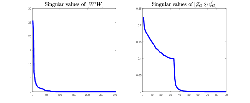
Figure 6. Experiment 1: The singular values of $[W^{*}W]$ and $[\vec{\varphi}_{G}\odot\vec{\psi}_{G}]$. The minimum singular values are $1.3448*10^{-15}$ and $2.5176*10^{-9}$, respectively.

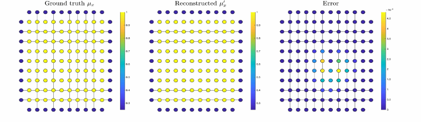
Figure 7. Experiment 1: The ground-truth $\mu_{x}$, the reconstructed $\mu_{x}^{\prime}$ and the absolute error. $\mathrm{L_{2}RNE}=1.0983*10^{-4}\%$.

Case 1.2: Gaussian Noise. Next, we validate the stability of the algorithm by adding Gaussian noise to the Neumann boundary spectral data. The noisy spectral data in use is of the form $\big{(}(1+\varepsilon)\lambda_{j},(1+\varepsilon)\phi_{j}|_{\partial G}\big{)}^{|G|}_{j=1}$, where $\phi$’s are the normalized Neumann eigenfunctions and $\varepsilon\sim\mathcal{N}(0,\sigma)$ is a zero mean Gaussian random variable/vector. We choose $\sigma\in[0.1\%,0.2\%,0.5\%]$ in the experiment, respectively.

In the presence of noise, the FRNEs for reconstructing $\Lambda_{\mu}$ are $0.086344\%$, $0.17\%$, $3.23\%$, respectively; the FRNEs for reconstructing $[W^{*}W]$ are $8.5562*10^{-2}\%$, $0.16\%$ , $4.78\%$, respectively. When applying the truncated SVD to solve (6.3), the thresholds for singular value truncation are $0.003,0.005,$ and $0.007$, respectively. When applying the truncated SVD to solve (6.4), the thresholds for singular value truncation are $0.001,0.001,$ and $0.003$, respectively. Here, different empirical thresholds are taken to achieve optimal results. The reconstruction $\mu^{\prime}_{x}$ and the absolute errors are shown in Fig.8, where the $\mathrm{L_{2}RNE}$s are $12.6\%$, $12.76\%$, $17.75\%$ respectively.

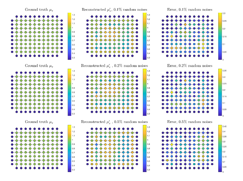
Figure 8. Experiment 1: Reconstructions and absolute errors in the presence of $0.1\%$, $0.2\%$ and $0.5\%$ Gaussian random noise. The $\mathrm{L_{2}RNE}$s are equal to $12.6\%$, $12.76\%$ and $17.75\%$ respectively. For comparison, we set the same color bar for the ground truth and the reconstruction.

7.2. Experiment 2 : the graph $T_{m,n}$

In this experiment, we set the following parameters: $m=10,n=9,|\partial G|=38,|G|=90,T=9$, $w_{x,y}=\frac{1}{2}(\mathrm{deg}(x)+\mathrm{deg}(y))$, and the ground-truth vertex weight is $\mu_{x}=1+0.5\sin(x)+0.5\cos(x)$ for all $x=1,2,\cdots,|\bar{G}|$.

Case 2.1: No Noise. We implement Algorithm 1 without noise to validate its efficacy. The $\mathrm{FRNE}$ between the reconstructed ND map $\Lambda_{\mu}^{\prime}$ using the Neumann boundary spectral data and the ground truth ND map $\Lambda_{\mu}$ is $3.3222*10^{-12}\%$.

When solving the equation (6.3), the matrix $[W^{*}W]$ is ill conditioned, see Fig. 9 for its singular values. We employ the truncated SVD regularization along with the ‘lsqminnorm’ command in MATLAB to find the minimum norm solution as $\vec{h}_{0}$. When solving the linear equations (6.4), we find that ${\rm rank}(\Delta_{G})=90$. By Lemma 5.2, we conclude the vectorized space of harmonic functions $\vec{H}$ has dimension $|\bar{G}|-rank(\Delta_{G})=38$. In this case, from MATLAB, there are $128$ linearly independent vectors of the form $\vec{\varphi}\odot\vec{\psi}$ with $\vec{\varphi},\vec{\psi}\in\vec{H}$. We use these $128$ linearly independent vectors as columns to construct the matrix $[\vec{\varphi}_{G}\odot\vec{\psi}_{G}]$ in order to solve (6.4). However, the matrix $[\vec{\varphi}_{G}\odot\vec{\psi}_{G}]$ is again ill conditioned, as is shown in Fig. 9, so we apply the truncated SVD regularization to find the minimum norm solution. The reconstruction and the error are shown in Fig. 10.

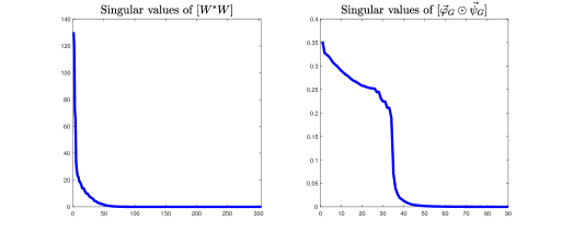
Figure 9. Experiment 2: The singular values of $[W^{*}W]$ and $[\vec{\varphi}_{G}\odot\vec{\psi}_{G}]$. The minimum singular values are $4.2386*10^{-15}$ and $1.1704*10^{-7}$, respectively.

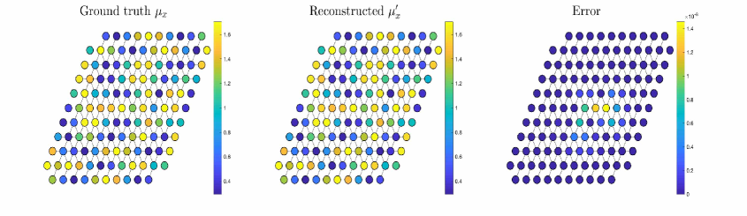
Figure 10. Experiment 2: The ground-truth $\mu_{x}$, the reconstructed $\mu_{x}^{\prime}$ and the absolute errors. $\mathrm{L_{2}RNE}=2.3817*10^{-7}\%$.

Case 2.2: Gaussian Noise. The noisy spectral data in use is of the form $\big{(}(1+\varepsilon)\lambda_{j},(1+\varepsilon)\phi_{j}|_{\partial G}\big{)}^{|G|}_{j=1}$, where $\phi$’s are the normalized Neumann eigenfunctions and $\varepsilon\sim\mathcal{N}(0,\sigma)$ is a zero mean Gaussian random variable/vector. We choose $\sigma\in[0.1\%,0.2\%,0.5\%]$ in the experiment, respectively.

In the presence of noise, the FRNEs for reconstructing $\Lambda_{\mu}$ are $\mathrm{FRNE}$s are $0.46\%$, $0.94\%$, $2.01\%$, respectively; the $\mathrm{FRNE}$s for reconstructing $[W^{*}W]$ are $0.38\%$, $0.8\%$, $1.02\%$, respectively. When applying the truncated SVD to solve (6.3), the thresholds for singular value truncation are $0.001$, $0.005$, and $0.003$, respectively. When applying the truncated SVD to solve (6.4), the thresholds for singular value truncation are $0.001,0.001$, and $0.003$, respectively. Here, different empirical thresholds are taken to achieve optimal results. The reconstruction $\mu^{\prime}_{x}$ and the absolute errors are shown in Fig. 11, where the $\mathrm{L_{2}RNE}$s are $27.81\%$, $28.17\%$ and $32.98\%$, respectively.

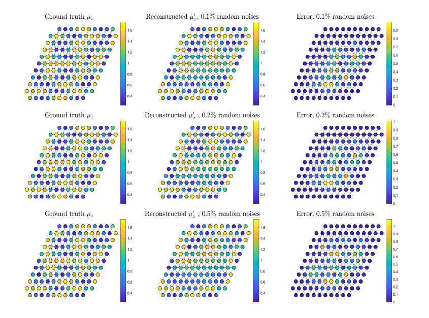
Figure 11. Experiment 2: Reconstructions and absolute errors in the presence of $0.1\%$, $0.2\%$ and $0.5\%$ Gaussian random noise. The $\mathrm{L_{2}RNE}$ are equal to $27.81\%$, $28.17\%$ and $32.98\%$ respectively. For comparison, we set the same color bar for the ground truth value and the reconstructed value.

7.3. Experiment 3 : the graph $H_{m,n}$

In this experiment, we set the following parameteres: $m=9,n=4,|\partial G|=28,|G|=90,T=9$, $w_{x,y}=\frac{1}{2}(\mathrm{deg}(x)+\mathrm{deg}(y))$ and the ground-truth vertex weight is $\mu_{x}=1$ for all $x\in\bar{G}$.

Case 3.1: No Noise. We implement Algorithm 1 without noise to validate its efficacy. The $\mathrm{FRNE}$ between the reconstructed ND map $\Lambda_{\mu}^{\prime}$ using the Neumann boundary spectral data and the ground truth ND map $\Lambda_{\mu}$ is $5.3689*10^{-13}\%$.

When solving the equation (6.3), the matrix $[W^{*}W]$ is ill conditioned, see Fig. 12 for its singular values. We employ the truncated SVD regularization along with the ‘lsqminnorm’ command in MATLAB to find the minimum norm solution as $\vec{h}_{0}$. When solve the linear equations (6.4), we find that ${\rm rank}(\Delta_{G})=90$. By Lemma 5.2, we conclude the vectorized space of harmonic functions $\vec{H}$ has dimension $|\bar{G}|-rank(\Delta_{G})=28$. In this case, from MATLAB, there are $118$ linearly independent vectors of the form $\vec{\varphi}\odot\vec{\psi}$ with $\vec{\varphi},\vec{\psi}\in\vec{H}$. Here, we use these $118$ linearly independent vectors as columns to construct the matrix $[\vec{\varphi}_{G}\odot\vec{\psi}_{G}]$ in order to solve (6.4). However, the matrix $[\vec{\varphi}_{G}\odot\vec{\psi}_{G}]$ is again ill conditioned, as is shown in Fig. 12, so we apply the truncated SVD regularization to find the minimum norm solution. The reconstruction and the errors are shown in Fig. 13.

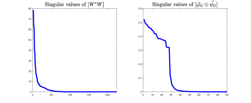
Figure 12. Experiment 3: The singular values of $[W^{*}W]$ and $[\vec{\varphi}_{G}\odot\vec{\psi}_{G}]$. The minimum singular values are $3.7372*10^{-15}$ and $1.1152*10^{-8}$, respectively.

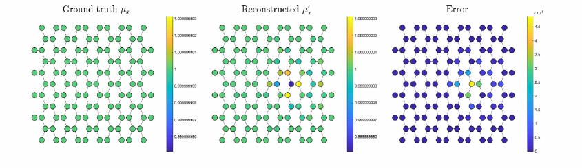
Figure 13. Experiment 3: The ground-truth $\mu_{x}$, the reconstructed $\mu_{x}^{\prime}$ and the errors. $\mathrm{L_{2}RNE}=7.7674*10^{-8}\%$.

Case 3.2: Gaussian Noise. The noisy spectral data in use is of the form $\big{(}(1+\varepsilon)\lambda_{j},(1+\varepsilon)\phi_{j}|_{\partial G}\big{)}^{|G|}_{j=1}$, where $\phi$’s are the normalized Neumann eigenfunctions and $\varepsilon\sim\mathcal{N}(0,\sigma)$ is a zero mean Gaussian random variable/vector. We choose $\sigma\in[0.1\%,0.2\%,0.5\%]$ in the experiment, respectively.

In the presence of noise, the FRNEs for reconstructing $\Lambda_{\mu}$ are $0.12\%$, $0.23\%$, $0.67\%$, respectively; the FRNEs for reconstructing $[W^{*}W]$ are $8.8772*10^{-2}\%$, $0.17\%$, $0.47\%$, respectively. When applying the truncated SVD to solve (6.3), the thresholds for singular value truncation are $0.001,0.005$, and $0.003$, respectively. When applying the truncated SVD to solve (6.4), the thresholds for singular value truncation are $0.001,0.001$, and $0.003$, respectively. Here, different empirical thresholds are taken to achieve optimal results. The reconstruction $\mu^{\prime}_{x}$ and the absolute errors are shown in Fig. 14, where the $\mathrm{L_{2}RNE}$s are $14.59\%$, $16.38\%$ and $24.89\%$ respectively.

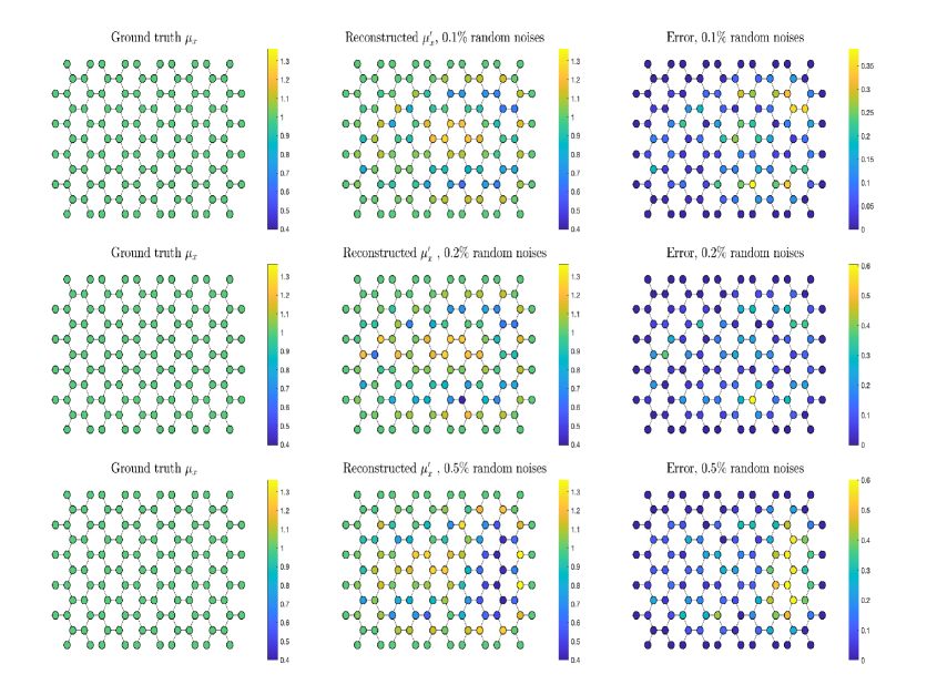
Figure 14. Experiment 3: Reconstructions and absolute errors in the presence of $0.1\%$, $0.2\%$ and $0.5\%$ Gaussian random noise. The $\mathrm{L_{2}RNE}$s are equal to $14.59\%$, $16.38\%$ and $24.89\%$ respectively. For comparison, we set the same color bar for the ground truth value and the reconstructed value.

Appendix A

In this article, we proved that the Neumann boundary spectral data determines (in a constructive way) the interior vertex weight under Assumption 1. On the other hand, the same conclusion is given in [11] with different assumptions on graphs. This appendix compares the two types of assumptions with the goal of highlighting their difference. In particular, we show that neither of the assumptions implies the other. As a result, our assumption identifies a novel class of graphs for which the discrete Gel’fand’s inverse spectral problem can be solved.

Recall some definitions and results in [11]. Let $\mathbb{G}$ be a finite graph with boundary. Let $G$ be the set of interior vertices of $\mathbb{G}$. A subset of these vertices is denoted by $X\subset G$ . A vertex $x\in X$ is called an extreme vertex of $X$ with respect to $\partial G$ if there exists a boundary vertex $z_{0}\in\partial G$ such that

$$d(x,z_{0})<\min_{y\in X,\,y\neq x}d(y,z_{0}).$$

In other words, $x$ is the unique nearest vertex in $X$ to $z_{0}$.

The major assumption on the graph in [11] is the following two conditions:

1. Any two interior vertices that are connected to the same boundary vertex are also connected to each other.

2. (Two-points condition) Any subset $X$ with $|X|\geq 2$ has at least two extreme vertices with respect to $\partial G$.

Note that Condition $(1)$ is void when a graph satisfies our Assumption 1$(i)$. Condition $(2)$ is referred to as the two-points condition in [11]. Moreover, the following criterion provides sufficient conditions for a graph to satisfy the two-points condition, see [11, Proposition 1.8].

Lemma A.1.

([11, Proposition 1.8]) If there exists a function $g:\bar{G}\rightarrow\mathbb{R}$ that satisfies the following conditions:

1. $|g(x)-g(y)|\leq 1$ when $x\sim y$;

2. for every $x\in G$, there is exactly one vertex $y_{1}\in\mathcal{N}(x)$ such that $g(y_{1})-g(x)=1$, and there is exactly one vertex $y_{2}\in\mathcal{N}(x)$ such that $g(y_{2})-g(x)=-1$;

3. for every $z\in\partial G$, there is at most one vertex $y_{3}\in\mathcal{N}(z)$ such that $g(y_{3})-g(z)=1$, and there is at most one vertex $y_{4}\in\mathcal{N}(z)$ such that $g(y_{4})-g(z)=-1$,

then the graph is said to satisfy the two-points condition.

We provide two specific graphs to show that the two sets of assumptions are different. First, there exist graphs that satisfy our Assumption 1 but not the two-points condition, see Fig. 15. This graph satisfies Assumption 1 because every vertex has no more than one next-level neighbor. However, the subset $X=\{x,y\}$ has just one extreme vertex $x$ with respect to $\partial G$. Any path between vertex $y$ and a boundary vertex must contain $x$. Therefore, $y$ cannot be the unique nearest vertex in $X$ to any boundary vertex.

On the other hand, there also exist graphs that satisfy the two-points condition but not our Assumption 1, see Fig. 15. For ease of notation, we constructed a Cartesian coordinate system in which the origin is marked, and the vertices are represented by the coordinates $(j,k)\in\mathbb{Z}^{2}$. This graph satisfies the two-points condition because the function $g(j,k)=\frac{j}{2}+k$ defined on $\bar{G}$ satisfies all the conditions in Lemma A.1. To demonstrate that it does not satisfy Assumption 1, note that

$$N_{1}=N_{1}^{1}\cup N_{1}^{2}\cup\{(2,3),(4,2)\}$$

where

$$N_{1}^{1}=\{(1,0),(1,3),(4,1),(4,5),(2,0),(3,0),(3,5)\},\qquad N_{1}^{2}=\{(1,1)\}.$$

Recall the definition of $N_{1}^{3}$ in Assumption 1, we find that $(2,3),(4,2)\not\in N_{1}^{3}$, because their next-level neighbors are respectively $(2,2),(3,3)$ and $(3,2),(4,3)$, none of which belong to $\mathcal{N}(N_{1}^{1}\cup N_{1}^{2})$. Therefore, the decomposition in Assumption 1 does not hold for this graph.

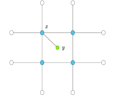
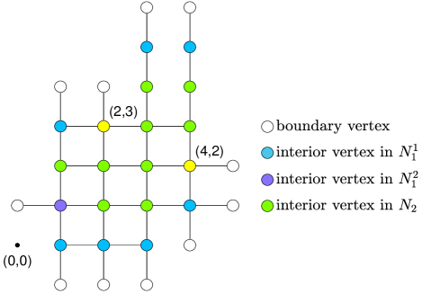
Figure 15. (a) A graph satisfies Assumption 1 but not the two-points condition. (b) A graph satisfies the two-points condition but not Assumption 1.

Appendix B

We compute some adjoint operators in this appendix. First, the linear operator

$$W:l^{2}(\{1,\cdots,T-1\}\times\partial G)\longmapsto l^{2}(G),\qquad h\longmapsto u^{P^{*}_{T}h}(T,x),~{}x\in G$$

is introduced in Section 4. It maps the Neumann boundary values to the solution of equation (1.5) at time $t=T$ and $x\in G$.

Lemma B.1.

The adjoint $W^{*}$ is given by

$$W^{*}g=v(t,z),\qquad(t,z)\in\{{1,2,\cdots,T-1\}\times\partial G}$$

where $v$ satisfies the following problem:

$$\begin{cases}D_{tt}v(t,x)-\Delta_{G}v(t,x)=0,&(t,x)\in\{1,2,\cdots,T-1\}\times G,\\ v(T,x)=0,&x\in\bar{G},\\ D_{t}v(T-1,x)=g(x),&x\in G,\\ \partial_{\nu}v(t,z)=0,&(t,z)\in\{0,1,\cdots,T\}\times\partial G.\end{cases}$$

Proof.

Let $u$ be the solution of (1.5). As $v$ satisfies the graph wave equation above, we have

$$0 =\sum\limits_{x\in G}\mu_{x}\sum\limits_{t=1}^{T-1}(D_{tt}v(t,x)-\Delta_{G}v(t,x))u(t,x)$$

$$=\sum\limits_{x\in G}\mu_{x}\sum\limits_{t=1}^{T-1}D_{tt}v(t,x)u(t,x)-\sum\limits_{x\in G}\mu_{x}\sum\limits_{t=1}^{T-1}u(t,x)\Delta_{G}v(t,x)$$

$$:=I_{1}-I_{2}.$$

For $I_{1}$, using the definition of the operators $D_{t}$ and $D_{tt}$, we can obtain

$$I_{1}= \sum\limits_{x\in G}\mu_{x}\sum\limits_{t=1}^{T-1}v(t+1,x)u(t,x)-2\sum\limits_{x\in G}\mu_{x}\sum\limits_{t=1}^{T-1}v(t,x)u(t,x)+\sum\limits_{x\in G}\mu_{x}\sum\limits_{t=1}^{T-1}v(t-1,x)u(t,x)$$

$$= \sum\limits_{x\in G}\mu_{x}\sum\limits_{t=1}^{T-1}(v(t,x)u(t-1,x)-2v(t,x)u(t,x)+v(t,x)u(t+1,x))$$

$$+\sum\limits_{x\in G}\mu_{x}(-v(1,x)u(0,x)+v(T,x)u(T-1,x)+v(0,x)u(1,x)-v(T-1,x)u(T,x))$$

$$= \sum\limits_{x\in G}\mu_{x}\sum\limits_{t=1}^{T-1}v(t,x)D_{tt}u(t,x)+\sum\limits_{x\in G}\mu_{x}g(x)u(T,x),$$

where we have used the fact that $u(0,x)=u(1,x)=0$, $v(T,x)=0$ and $v(T-1,x)=-g(x)$ for $x\in G$.

For $I_{2}$, we compute it using Lemma 3.1:

$$I_{2} =\sum\limits_{x\in G}\mu_{x}\sum\limits_{t=1}^{T-1}v(t,x)\Delta_{G}u(t,x)+\sum\limits_{z\in\partial G}\mu_{z}\sum\limits_{t=1}^{T-1}(v(t,z)\partial_{\nu}u(t,z)-u(t,z)\partial_{\nu}v(t,z))$$

$$=\sum\limits_{x\in G}\mu_{x}\sum\limits_{t=1}^{T-1}v(t,x)\Delta_{G}u(t,x)+\sum\limits_{z\in\partial G}\mu_{z}\sum\limits_{t=1}^{T-1}v(t,z)f(t,z),$$

where we have used the boundary conditions $\partial_{\nu}v(t,z)=0$ and $\partial_{\nu}u(t,z)=f$ for $z\in\partial G$.

As $I_{1}-I_{2}=0$ and the first terms of $I_{1}$ and $I_{2}$ are identical, we conclude:

$$\sum_{z\in\partial G}\mu_{z}\sum_{t=1}^{T-1}v(t,z)f(t,z)=\sum\limits_{x\in G}\mu_{x}g(x)u(T,x)=(u(T),g)_{G}=(Wf,g)_{G}.$$

The proof is complete when we observe that the left hand side is exactly $(f,v)_{\{1,\cdots,T-1\}\times\partial G}$.

∎

B.1. Calculate the map $\Lambda_{\mu,T}^{*}$

Next, we derive the adjoint to the operator $\Lambda_{\mu,T}$ introduced in Section 4. Recall that

$$\Lambda_{\mu,T}h:=P_{T}(\Lambda_{\mu}P_{T}^{*}h)=u^{P_{T}^{*}h}|_{\{1,\cdots,T-1\}\times\partial G}$$

for $h\in l^{2}({\{1,\cdots,T-1\}\times\partial G})$.

Lemma B.2.

The adjoint $\Lambda^{*}_{\mu,T}$ is given by

$$\Lambda_{\mu,T}^{*}=\mathscr{R}\Lambda_{\mu,T}\mathscr{R}.$$

Proof.

Let $u$ be the solution of (1.5) and $v$ be the solution of

$$\begin{cases}D_{tt}v(t,x)-\Delta_{G}v(t,x)=0,&(t,x)\in\{1,\cdots,T-1\}\times G,\\ v(T-1,x)=0,&x\in\bar{G},\\ D_{t}v(T-1,x)=0,&x\in G,\\ \partial_{\nu}v(t,z)=g(t,z),&(t,z)\in\{0,\cdots,T\}\times\partial G.\end{cases}$$

Using Lemma 3.1, we obtain the equation

$$0= \sum\limits_{x\in G}\mu_{x}\sum\limits_{t=1}^{T-1}(D_{tt}v(t,x)-\Delta_{G}v(t,x))u(t,x)$$

$$= \sum\limits_{x\in G}\mu_{x}\sum\limits_{t=1}^{T-1}D_{tt}v(t,x)u(t,x)-\sum\limits_{x\in G}\mu_{x}\sum\limits_{t=1}^{T-1}\Delta_{G}v(t,x)u(t,x)$$

$$= \sum\limits_{x\in G}\mu_{x}\sum\limits_{t=1}^{T-1}(v(t,x)u(t-1,x)-2v(t,x)u(t,x)+v(t,x)u(t+1,x))$$

$$+\sum\limits_{x\in G}\mu_{x}(-v(1,x)u(0,x)+v(T,x)u(T-1,x)+v(0,x)u(1,x)-v(T-1,x)u(T,x))$$

$$-\sum\limits_{x\in G}\mu_{x}\sum\limits_{t=1}^{T-1}v\Delta_{G}u+\sum\limits_{z\in\partial G}\mu_{z}\sum\limits_{t=1}^{T-1}(\partial_{\nu}v(t,z)u(t,z)-v(t,z)\partial_{\nu}u(t,z))$$

$$= \sum\limits_{x\in G}\mu_{x}\sum\limits_{t=1}^{T-1}v(t,x)(D_{tt}u(t,x)-\Delta_{G}u(t,x))+\sum\limits_{z\in\partial G}\mu_{z}\sum\limits_{t=1}^{T-1}(\partial_{\nu}v(t,z)u(t,z)-v(t,z)\partial_{\nu}u(t,z))$$

$$= \sum\limits_{z\in\partial G}\mu_{z}\sum\limits_{t=1}^{T-1}g(\Lambda_{\mu,T}f)-\sum\limits_{z\in\partial G}\mu_{z}\sum\limits_{t=1}^{T-1}v(t,z)f.$$ (B.1)

On the other hand, consider $U$ that satisfies the following problem

$$\begin{cases}D_{tt}U(t,x)-\Delta_{G}U(t,x)=0,&(t,x)\in\{1,\cdots,T-1\}\times G,\\ U(0,x)=0,&x\in\bar{G},\\ D_{t}U(0,x)=0,&x\in G,\\ \partial_{\nu}U(t,z)=\mathscr{R}g(t,z),&(t,z)\in\{0,\cdots,T\}\times\partial G.\end{cases}$$

Then, $\mathscr{R}U=v$, since they solve the initial boundary value problem. We conclude

$$\mathscr{R}\Lambda_{\mu,T}\mathscr{R}g=\mathscr{R}(U|_{\{1,\cdots,T-1\}\times\partial G})=v|_{\{1,\cdots,T-1\}\times\partial G}.$$

Substitute this relation into equation (B.1) to get

$$0 =\sum\limits_{z\in\partial G}\mu_{z}\sum\limits_{t=1}^{T-1}g(\Lambda_{\mu,T}f)-\sum\limits_{z\in\partial G}\mu_{z}\sum\limits_{t=1}^{T-1}f\mathscr{R}\Lambda_{\mu,T}\mathscr{R}g$$

$$=(\Lambda_{\mu,T}f,g)_{\{1,\cdots,T-1\}\times\partial G}-(f,\mathscr{R}\Lambda_{\mu,T}\mathscr{R}g)_{\{1,\cdots,T-1\}\times\partial G}$$

for all $f,g$. This completes the proof.

∎

Appendix C

C.1. Matrix form of the graph Laplacian operator $\Delta_{G}$

In this appendix, we use the matrix form of the graph Laplacian to prove a few auxiliary results. As usual, we index the interior vertices by $x_{1},x_{2},\cdots,x_{|G|}$ and the boundary vertices by $x_{|G|+1},x_{|G|+2},\cdots,x_{|\bar{G}|}$ on $\bar{G}$. Recall that in Section 5, the graph Laplacian $\Delta_{G}:\bar{G}\rightarrow G$ is identified with a block matrix

$$[\Delta_{G}]=([\Delta_{G,G}],[\Delta_{G,\partial G}])\;\in\mathbb{R}^{|G|\times|\bar{G}|},\quad\text{ where }[\Delta_{G,G}]\in\mathbb{R}^{|G|\times|G|},\;[\Delta_{G,\partial G}]\in\mathbb{R}^{|G|\times|\partial G|}.$$

Then, the graph Laplacian operator $\Delta_{G}$ can be written as matrix form as follows

$$\begin{split}\begin{pmatrix}\frac{-\sum\limits_{\begin{subarray}{c}y\in\bar{G}\\ y\sim{x_{1}}\end{subarray}}w(x_{1},y)}{\mu_{x_{1}}}&\frac{w(x_{1},x_{2})}{\mu_{x_{1}}}&\cdots&\frac{w(x_{1},x_{|G|})}{\mu_{x_{1}}}&\cdots&\frac{w(x_{1},x_{|\bar{G}|})}{\mu_{x_{1}}}\\ \frac{w(x_{2},x_{1})}{\mu_{x_{2}}}&\frac{-\sum\limits_{\begin{subarray}{c}y\in\bar{G}\\ y\sim{x_{2}}\end{subarray}}w(x_{2},y)}{\mu_{x_{2}}}&\cdots&\frac{w(x_{2},x_{|G|})}{\mu_{x_{2}}}&\cdots&\frac{w(x_{2},x_{|\bar{G}|})}{\mu_{x_{2}}}\\ \vdots&\vdots&&\vdots&&\vdots\\ \frac{w(x_{|G|},x_{1})}{\mu_{x_{|G|}}}&\frac{w(x_{|G|},x_{2})}{\mu_{x_{|G|}}}&\cdots&\frac{-\sum\limits_{\begin{subarray}{c}y\in\bar{G}\\ y\sim{x_{|G|}}\end{subarray}}w(x_{|G|},y)}{\mu_{x_{|G|}}}&\cdots&\frac{w(x_{|G|},x_{|\bar{G}|})}{\mu_{x_{|G|}}}\\ \end{pmatrix}:=\begin{pmatrix}\Delta_{G,G}&\vdots&\Delta_{G,\partial G}\end{pmatrix},\end{split}$$

where

$$\begin{split}\Delta_{G,G}=\begin{pmatrix}\frac{1}{\mu_{x_{1}}}&\\ &\frac{1}{\mu_{x_{2}}}\\ &&\ddots&\\ &&&\frac{1}{\mu_{x_{|G|}}}\end{pmatrix}\begin{pmatrix}-\sum\limits_{\begin{subarray}{c}y\in\bar{G}\\ y\sim{x_{1}}\end{subarray}}w(x_{1},y)&w(x_{1},x_{2})&\cdots&w(x_{1},x_{|G|})\\ w(x_{2},x_{1})&-\sum\limits_{\begin{subarray}{c}y\in\bar{G}\\ y\sim{x_{2}}\end{subarray}}w(x_{2},y)&\cdots&w(x_{2},x_{|G|})\\ \vdots&\vdots&&\vdots\\ w(x_{|G|},x_{1})&w(x_{|G|},x_{2})&\cdots&-\sum\limits_{\begin{subarray}{c}y\in\bar{G}\\ y\sim{x_{|G|}}\end{subarray}}w(x_{|G|},y)\end{pmatrix},\end{split}$$

and

$$\begin{split}\Delta_{G,\partial G}=\begin{pmatrix}\frac{1}{\mu_{x_{1}}}&\\ &\frac{1}{\mu_{x_{2}}}\\ &&\ddots&\\ &&&\frac{1}{\mu_{x_{|G|}}}\end{pmatrix}\begin{pmatrix}w(x_{1},x_{|G|+1})&\cdots&w(x_{1},x_{|\bar{G}|})\\ w(x_{2},x_{|G|+1})&\cdots&w(x_{2},x_{|\bar{G}|})\\ \vdots&&\vdots\\ w(x_{|G|},x_{|G|+1})&\cdots&w(x_{|G|},x_{|\bar{G}|})\end{pmatrix}.\end{split}$$

Since the edge weight function $w(\cdot,\cdot)$ is symmetric, the resulting matrix $\Delta_{G,G}$ is also symmetric.

Lemma C.1.

For any function $g:\partial G\rightarrow\mathbb{R}$, the boundary value problem

$$\Delta_{G}\varphi(x)=0~{}\text{ for }~{}x\in G,\qquad\varphi|_{\partial G}=g$$

has a unique solution $\varphi:\bar{G}\to\mathbb{R}$.

Proof.

Using the vectorization $\vec{\varphi}=(\vec{\varphi}|_{G},\vec{g})^{T}$ and the matrix $[\Delta_{G}]=([\Delta_{G,G}],[\Delta_{G,\partial G}])$, the boundary value problem is equivalent to the homogeneous linear system

$$\left(\begin{array}[]{cc}[\Delta_{G,G}],&[\Delta_{G,\partial G}]\end{array}\right)\left(\begin{array}[]{c}\vec{\varphi}|_{G}\\ \vec{g}\end{array}\right)=0.$$

Since the matrix $[\Delta_{G,G}]$ is non-singular [19, Lemma 3.8], the linear system admits a unique solution

$$\vec{\varphi}|_{G}=-[\Delta_{G,G}]^{-1}[\Delta_{G,\partial G}]\vec{g}.$$

∎

Lemma C.2.

Let $\beta$ be an arbitrary selection of $|G|$ columns from $\mathbf{H}$. If $\det(\mathbf{H}_{:,\beta})\neq 0$, then $\det(\mathbf{H}_{:,\beta})$ is a real analytic function of $\{w_{x,y}\}\in\mathbb{R}_{+}^{|\mathcal{E}|}$.

Proof.

Using the cofactor formula, each entry of $[\Delta_{G,G}]^{-1}$ is a rational function of $\{w_{x,y}\}\in\mathbb{R}_{+}^{|\mathcal{E}|}$ (since $\det[\Delta_{G,G}]$ is a polynomial of the entries). Recall that for polynomials $A_{1}(a)$ and $A_{2}(a)\neq 0$ when $a\in\mathbb{R}^{|\mathcal{E}|}$, rational functions of the form $\frac{A_{1}(a)}{A_{2}(a)}$ are analytic on any connected subset of $\mathbb{R}^{|\mathcal{E}|}$. Since $\Delta_{G,G}$ is invertible, the functions $\det(\mathbf{H}_{:,\beta})$ are real analytic with respect to $\{w_{x,y}\}\in\mathbb{R}_{+}^{|\mathcal{E}|}$. ∎

References

- [1] M. Anderson, A. Katsuda, Y. Kurylev, M. Lassas, and M. Taylor. Boundary regularity for the Ricci equation, geometric convergence, and Gel’fand’s inverse boundary problem. Invent. Math., 158(2):261–321, 2004.
- [2] S. A. Avdonin and V. V. Kravchenko. Method for solving inverse spectral problems on quantum star graphs. J. Inverse Ill-Posed Probl., 31(1):31–42, 2023.
- [3] M. I. Belishev. An approach to multidimensional inverse problems for the wave equation. Dokl. Akad. Nauk SSSR, 297(3):524–527, 1987.
- [4] M. I. Belishev. Boundary spectral inverse problem on a class of graphs (trees) by the BC method. Inverse Problems, 20(3):647–672, 2004.
- [5] M. I. Belishev. Recent progress in the boundary control method. Inverse Problems, 23(5):R1–R67, 2007.
- [6] M. I. Belishev and V. Y. Gotlib. Dynamical variant of the BC-method: theory and numerical testing. J. Inverse Ill-Posed Probl., 7(3):221–240, 1999.
- [7] M. I. Belishev, I. B. Ivanov, I. V. Kubyshkin, and V. S. Semenov. Numerical testing in determination of sound speed from a part of boundary by the BC-method. J. Inverse Ill-Posed Probl., 24(2):159–180, 2016.
- [8] M. I. Belishev and Y. V. Kurylev. To the reconstruction of a Riemannian manifold via its spectral data (BC-method). Comm. Partial Differential Equations, 17(5-6):767–804, 1992.
- [9] M. I. Belishev and A. F. Vakulenko. Inverse problems on graphs: recovering the tree of strings by the BC-method. J. Inverse Ill-Posed Probl., 14(1):29–46, 2006.
- [10] M. I. Belishev and N. Wada. On revealing graph cycles via boundary measurements. Inverse Problems, 25(10):105011, 21, 2009.
- [11] E. Blå sten, H. Isozaki, M. Lassas, and J. Lu. Gelfand’s inverse problem for the graph Laplacian. J. Spectr. Theory, 13(1):1–45, 2023.
- [12] E. Blå sten, H. Isozaki, M. Lassas, and J. Lu. Inverse problems for discrete heat equations and random walks for a class of graphs. SIAM J. Discrete Math., 37(2):831–863, 2023.
- [13] A. S. Blagoveshchenskii. The Inverse Problem in the Theory of Seismic Wave Propagation, pages 55–67. Springer US, Boston, MA, 1967.
- [14] J. Boyer, J. J. Garzella, and F. Guevara Vasquez. On the solvability of the discrete conductivity and Schrödinger inverse problems. SIAM J. Appl. Math., 76(3):1053–1075, 2016.
- [15] D. Burago, S. O. Ivanov, M. Lassas, and J. Lu. Quantitative stability of Gel’fand’s inverse boundary problem. arXiv:2012.04435.
- [16] A.-P. Calderón. On an inverse boundary value problem. In Seminar on Numerical Analysis and its Applications to Continuum Physics (Rio de Janeiro, 1980), pages 65–73. Soc. Brasil. Mat., Rio de Janeiro, 1980.
- [17] A. Chernyshenko and V. Pivovarchik. Recovering the shape of a quantum graph. Integr. Equ. Oper. Theory, 92(3):Paper No. 23, 17, 2020.
- [18] M. Choulli and P. Stefanov. Stability for the multi-dimensional Borg-Levinson theorem with partial spectral data. Comm. Partial Differential Equations, 38(3):455–476, 2013.
- [19] E. B. Curtis and J. A. Morrow. Inverse problems for electrical networks, volume 13 of Ser. Appl. Math., Singap. River Edge, NJ: World Scientific, 2000.
- [20] D. M. Cvetković, M. Doob, I. Gutman, and A. Torgašev. Recent results in the theory of graph spectra, volume 36 of Ann. Discrete Math. North-Holland Publishing Co., Amsterdam, 1988.
- [21] M. V. de Hoop, P. Kepley, and L. Oksanen. Recovery of a smooth metric via wave field and coordinate transformation reconstruction. SIAM Journal on Applied Mathematics, 78(4):1931–1953, 2018.
- [22] H. Fujii and A. Katsuda. Isospectral graphs and isoperimetric constants. Discrete Math., 207(1-3):33–52, 1999.
- [23] I. Gelfand. Some aspects of functional analysis and algebra. In Proceedings of the International Congress of Mathematicians, Amsterdam, 1954, Vol. 1, pages 253–276. Erven P. Noordhoff N. V., Groningen; North-Holland Publishing Co., Amsterdam, 1957.
- [24] B. Gutkin and U. Smilansky. Can one hear the shape of a graph? J. Phys. A, 34(31):6061–6068, 2001.
- [25] H. Isozaki. Some remarks on the multi-dimensional Borg-Levinson theorem. J. Math. Kyoto Univ., 31(3):743–753, 1991.
- [26] H. Isozaki and E. Korotyaev. Inverse problems, trace formulae for discrete Schrödinger operators. Ann. Henri Poincaré, 13(4):751–788, 2012.
- [27] A. P. Kachalov and Y. V. Kurylev. The multidimensional inverse Gel’fand problem with incomplete boundary spectral data. Dokl. Akad. Nauk, 346(5):587–589, 1996.
- [28] A. Katchalov and Y. Kurylev. Multidimensional inverse problem with incomplete boundary spectral data. Comm. Partial Differential Equations, 23(1-2):55–95, 1998.
- [29] A. Katchalov, Y. Kurylev, and M. Lassas. Inverse boundary spectral problems, volume 123 of Chapman & Hall/CRC Monographs and Surveys in Pure and Applied Mathematics. Chapman & Hall/CRC, Boca Raton, FL, 2001.
- [30] A. Katchalov, Y. Kurylev, M. Lassas, and N. Mandache. Equivalence of time-domain inverse problems and boundary spectral problems. Inverse Problems, 20(2):419–436, 2004.
- [31] A. Katsuda, Y. Kurylev, and M. Lassas. Stability and reconstruction in Gel’fand inverse boundary spectral problem. In New analytic and geometric methods in inverse problems, pages 309–322. Springer, Berlin, 2004.
- [32] J. Korpela, M. Lassas, and L. Oksanen. Discrete regularization and convergence of the inverse problem for 1+1 dimensional wave equation. Inverse Problems & Imaging, 13(3):575–596, 2019.
- [33] P. Kurasov and M. Nowaczyk. Inverse spectral problem for quantum graphs. J. Phys. A, 38(22):4901–4915, 2005.
- [34] Y. Kurylev and M. Lassas. Multidimensional Gel’fand inverse boundary spectral problem: uniqueness and stability. Cubo, 8(1):41–59, 2006.
- [35] Y. V. Kurylev and M. Lassas. The multidimensional Gel’fand inverse problem for non-self-adjoint operators. Inverse Problems, 13(6):1495–1501, 1997.
- [36] D.-Q. Liu and C.-F. Yang. Inverse spectral problems for Dirac operators on a star graph with mixed boundary conditions. Math. Methods Appl. Sci., 44(13):10663–10672, 2021.
- [37] B. S. Mityagin. The zero set of a real analytic function. Mat. Zametki, 107(3):473–475, 2020.
- [38] A. Nachman, J. Sylvester, and G. Uhlmann. An -dimensional Borg-Levinson theorem. Comm. Math. Phys., 115(4):595–605, 1988.
- [39] L. Oksanen, T. Yang, and Y. Yang. Linearized boundary control method for an acoustic inverse boundary value problem. Inverse Problems, 38(11):114001, 2022.
- [40] L. Oksanen, T. Yang, and Y. Yang. Linearized boundary control method for density reconstruction in acoustic wave equations. arXiv:2405.14989v1, 2024.
- [41] J. Tan. On isospectral graphs. Interdiscip. Inform. Sci., 4(2):117–124, 1998.
- [42] D. Tataru. Unique continuation for solutions to PDE’s; between Hörmander’s theorem and Holmgren’s theorem. Comm. Partial Differential Equations, 20(5-6):855–884, 1995.
- [43] S. V. Vasilev. An inverse spectral problem for Sturm-Liouville operators with singular potentials on graphs with a cycle. Izv. Sarat. Univ. (N.S.) Ser. Mat. Mekh. Inform., 19(4):366–376, 2019.
- [44] C.-F. Yang. Inverse spectral problems for the Sturm-Liouville operator on a -star graph. J. Math. Anal. Appl., 365(2):742–749, 2010.
- [45] T. Yang and Y. Yang. A stable non-iterative reconstruction algorithm for the acoustic inverse boundary value problem. Inverse Probl. Imaging, 16(1):1–18, 2022.
- [46] V. Yurko. Inverse spectral problems for Sturm-Liouville operators on graphs. Inverse Problems, 21(3):1075–1086, 2005.