Application of Machine Learning and Convex Limiting to Subgrid Flux Modeling in the Shallow-Water Equations

Abstract

We propose a combination of machine learning and flux limiting for property-preserving subgrid scale modeling in the context of flux-limited finite volume methods for the one-dimensional shallow-water equations. The numerical fluxes of a conservative target scheme are fitted to the coarse-mesh averages of a monotone fine-grid discretization using a neural network to parametrize the subgrid scale components. To ensure positivity preservation and the validity of local maximum principles, we use a flux limiter that constrains the intermediate states of an equivalent fluctuation form to stay in a convex admissible set. The results of our numerical studies confirm that the proposed combination of machine learning with monolithic convex limiting produces meaningful closures even in scenarios for which the network was not trained.

Key words: shallow water equations; large eddy simulation; subgrid scale modeling; parametrization; neural networks; positivity preservation; flux limiting

1 Introduction

Many fluid flow models are based on nonlinear conservation laws that incorporate a vast range of spatial and temporal scales. Therefore, direct numerical simulations are often prohibitively expensive and, despite rapid progress in computer architecture, existing codes cannot be run at the discretization level required to resolve all relevant physical processes. Therefore, the derivation/calibration of reduced models has been an active area of research for many decades. The simplest Large-Eddy Simulation (LES) approaches use the Smagorinsky eddy viscosity model [40] for subgrid stresses that appear in the spatially filtered equations. More advanced alternatives include stochastic (e.g. [25, 32, 7, 21, 10, 41, 6, 35]) and deterministic (e.g. [1, 12, 27, 33]) closures, alpha models [20] etc. Recently, machine learning has also been used to represent the effects of unresolved degrees of freedom (e.g. [8, 3, 43, 2], review [28]).

The main focus of our work is on the Shallow-Water Equations (SWE) [36]. This nonlinear hyperbolic system is widely used to simulate flow in rivers and channels, as well as coastal and ocean dynamics. In the context of ocean dynamics, parametrization of mesoscale eddies requires developing appropriate subgrid scale models. Recent years have witnessed the advent of closures based on Machine Learning (ML). The validity and effectiveness of such modern closures was demonstrated by many numerical examples. However, the use of Neural Network (NN) approximations makes it more difficult to prove the stability, consistency, and convergence of ML numerical methods for nonlinear PDEs. Moreover, for the SWE model, an NN-based closure may violate entropy inequalities or produce negative water heights. As a fail-safe remedy, we consider an NN model for representing subgrid fluxes (instead of estimating the whole right-hand side of the reduced model) and propose the application of a physics-aware flux limiter to ML-generated subgrid fluxes that may violate important inequality constraints. We use a relatively simple feed-forward network to extract subgrid fluxes from data generated by the fully resolved model. The monolithic convex limiting (MCL) strategy [22] that we use in this work represents the coarse-mesh cell averages as convex combinations of intermediate states that belong to a convex admissible set. The proofs of desired properties exploit this fact following the analysis of flux-corrected transport (FCT) algorithms by Guermond et al. [15].

The rest of the paper is organized as follows. We define the conserved variables and fluxes of the one-dimensional SWE system in Section 2. The space discretization of this nonlinear hyperbolic system and the definition of coarse-scale variables are discussed in Section 3. The fine-mesh discretization uses the Local Lax–Friedrichs (LLF) flux and is bound preserving. In Section 3.1, we construct the subgrid fluxes of the coarse-mesh model using a neural network. The MCL framework that we present in Section 3.2 is used for flux limiting purposes. In Section 4, we perform numerical experiments. The results of fully resolved simulations are compared with NN-based reduced model approximations. The effect of locally bound-preserving MCL corrections is studied by switching the flux limiter on and off. Conclusions are drawn in Section 5.

2 Shallow-Water Equations

We consider the one-dimensional SWE system with periodic boundary conditions imposed on the boundaries of the domain $\Omega=(0,L)$. The evolution of the fluid depth $h(x,t)$ and fluid velocity $v(x,t)$ is governed by

$$\begin{bmatrix}h\\ hv\end{bmatrix}_{t}+\begin{bmatrix}hv\\ hv^{2}+\frac{1}{2}gh^{2}\end{bmatrix}_{x}=0,$$ (1)

where $x\in\bar{\Omega}$ is the space variable, $t\geq 0$ is the time variable, and $g$ is the gravitational acceleration. The initial conditions are given by $h(x,0)=h_{0}(x)$, $v(x,0)=v_{0}(x).$ We assume that $h(x,t)>0$, i.e., no dry states are present. Introducing the discharge $q=hv$, the hyperbolic system (1) can be rewritten as

$$\begin{bmatrix}h\\ q\end{bmatrix}_{t}+\begin{bmatrix}q\\ q^{2}/h+\frac{1}{2}gh^{2}\end{bmatrix}_{x}=0.$$ (2)

This is a system of the form $u_{t}+(f(u))_{x}=0$, where $u=[h,q]^{T}$ is the vector of conserved quantities and $f(u)=[q,q^{2}/h+\frac{1}{2}gh^{2}]^{T}$ is the flux function. We initialize $u$ by $u_{0}=[h_{0},q_{0}]^{T}$, where $q_{0}=h_{0}v_{0}$.

3 Discretization, Coarse-Scale Variables, and Subgrid Fluxes

A finite-volume discretization of the SWE system on a uniform fine mesh with spacing $\Delta x=L/N_{f}$ produces a system of ordinary differential equations

$$\frac{\mathrm{d}}{\mathrm{d}t}u_{i}=\frac{F_{i-\nicefrac{{1}}{{2}}}-F_{i+\nicefrac{{1}}{{2}}}}{\Delta x}\qquad i=1,\ldots,N_{f}$$ (3)

for approximate fine-mesh cell averages $u_{i}(t)\approx\frac{1}{\Delta x}\int_{x_{i-\nicefrac{{1}}{{2}}}}^{x_{i+\nicefrac{{1}}{{2}}}}u(x,t)\mathrm{d}x$. The numerical flux

$$F_{i+\nicefrac{{1}}{{2}}}=\frac{f(u_{i})+f(u_{i+1})}{2}-\frac{\lambda_{i+\nicefrac{{1}}{{2}}}}{2}(u_{i+1}-u_{i})$$ (4)

of the Local Lax-Friedrichs (LLF) scheme is defined using the maximum wave speed $\lambda_{i+\nicefrac{{1}}{{2}}}$ of the Riemann problem with the initial states $u_{i}$ and $u_{i+1}$. The intermediate state

$$\bar{u}_{i+\nicefrac{{1}}{{2}}}:=\frac{u_{i+1}+u_{i}}{2}-\frac{1}{2\lambda_{i+\nicefrac{{1}}{{2}}}}(f(u_{i+1})-f(u_{i}))$$ (5)

represents a spatially averaged exact solution of such a Riemann problem. In what follows, the state $\bar{u}_{i+\nicefrac{{1}}{{2}}}$ is referred to as a bar state. Using the maximum eigenvalue of the Jacobian matrices $f^{\prime}(u_{i})$ and $f^{\prime}(u_{i+1})$ as an approximate upper bound for the local wave speed, we set [26]

$$\lambda_{i+\nicefrac{{1}}{{2}}}:=\max\left(\lvert v_{i}\rvert+\sqrt{gh_{i}},\,\lvert v_{i+1}\rvert+\sqrt{gh_{i+1}}\right).$$ (6)

We denote by $\mathcal{F}(u_{L},u_{R})$ the numerical flux function such that $F_{i+\nicefrac{{1}}{{2}}}=\mathcal{F}(u_{i},u_{i+1})$ is given by (4) with $\lambda_{i+\nicefrac{{1}}{{2}}}$ defined by (6). Substituting the so-defined LLF flux into (3) and invoking the definition (5) of $\bar{u}_{i+\nicefrac{{1}}{{2}}}$, we write the spatial semi-discretization (3) in the equivalent fluctuation form (cf. [26])

$$\frac{\mathrm{d}}{\mathrm{d}t}u_{i}=\frac{1}{\Delta x}\bigl{[}\lambda_{i-\nicefrac{{1}}{{2}}}(\bar{u}_{i-\nicefrac{{1}}{{2}}}-u_{i})+\lambda_{i+\nicefrac{{1}}{{2}}}(\bar{u}_{i+\nicefrac{{1}}{{2}}}-u_{i})\bigr{]},\qquad i=1,\ldots,N_{f}.$$ (7)

In this paper, we utilize Heun’s time-stepping method. This explicit two-step Runge-Kutta scheme is second-order accurate and yields a convex combination of two forward Euler predictors. Heun’s method is a representative of strong stability preserving (SSP) methods [39, 14, 13]. The resulting space-time discretization also belongs to the class of height positivity preserving (HPP) methods, i.e., the fully discrete scheme guarantees that the water height $h_{i}(t)$ remains strictly positive for all times (see [38] for details).

We assume that the fine-mesh discretization resolves all physical processes of interest sufficiently well. This, essentially, implies that the number $N_{f}$ of fine mesh cells

$$C_{i}=[x_{i-\nicefrac{{1}}{{2}}},x_{i+\nicefrac{{1}}{{2}}}],\quad i=1,\ldots,N_{f}$$

is very large and the numerical viscosity introduced by the LLF scheme is very small. To avoid the high cost of direct numerical simulations on the fine mesh, we compose a coarse mesh from macrocells

$$\bar{C}_{i}:=\bigcup_{j=k(i-1)+1}^{ki}C_{j}=[x_{k(i-1)+\nicefrac{{1}}{{2}}},\,x_{ki+\nicefrac{{1}}{{2}}}],\qquad i=1,\ldots,N_{c},$$ (8)

where $k$ is the coarsening degree, $N_{c}=N_{f}/k$, and $\Delta X=k\Delta x$. The coarse-scale variables

$$U_{i}(t)=\frac{1}{k}\sum_{j=k(i-1)+1}^{ki}u_{j}(t),\qquad i=1,\ldots,N_{c}$$ (9)

correspond to averages over the macrocells $\bar{C}_{i}$. In principle, we could use the LLF finite volume discretization of the integral conservation law for $\bar{C}_{i}$ to directly obtain an evolution equation for $U_{i}$. However, a coarse-mesh LLF approximation is unlikely to resolve all physical processes appropriately even for moderate values of the parameter $k$. To derive subgrid fluxes that significantly reduce the error of the coarse-grid LLF scheme, we need to average equations (7). The resulting equation for $U_{i}$ can be written in the form

$$\frac{\mathrm{d}}{\mathrm{d}t}U_{i}=\frac{(\bar{F}_{i-\nicefrac{{1}}{{2}}}+G_{i-\nicefrac{{1}}{{2}}})-(\bar{F}_{i+\nicefrac{{1}}{{2}}}+G_{i+\nicefrac{{1}}{{2}}})}{\Delta X},$$ (10)

where $\bar{F}_{i+\nicefrac{{1}}{{2}}}=\mathcal{F}(U_{i},U_{i+1})$ is the coarse-mesh LLF flux. The fine-scale component of the subgrid flux

$$G_{i+\nicefrac{{1}}{{2}}}:=F_{ki+\nicefrac{{1}}{{2}}}-\bar{F}_{i+\nicefrac{{1}}{{2}}}$$ (11)

is given by $F_{ki+\nicefrac{{1}}{{2}}}=\mathcal{F}(u_{ki},u_{ki+1})$. The point $X_{i+1/2}=x_{ki+\nicefrac{{1}}{{2}}}$ represents the interface of fine-mesh cells $C_{ki}$ and $C_{ki+1}$ such that $C_{ki}\cap C_{ki+1}=\bar{C}_{i}\cap\bar{C}_{i+1}$. The flux defined by (11) can be also expressed as

$$G_{i+\nicefrac{{1}}{{2}}}:=\mathcal{G}(u_{ki},u_{ki+1},U_{i},U_{i+1})=\mathcal{F}(u_{ki},u_{ki+1})-\mathcal{F}(U_{i},U_{i+1}).$$ (12)

In general, the subgrid flux depends on the coarse-scale variables and the fine-mesh cell averages. The evolution equation (10) has the structure of a finite-volume discretization of the SWE system on a coarse mesh. The coarse-mesh LLF discretization without the subgrid fluxes is given by

$$\frac{\mathrm{d}}{\mathrm{d}t}U_{i}=\frac{\bar{F}_{i-\nicefrac{{1}}{{2}}}-\bar{F}_{i+\nicefrac{{1}}{{2}}}}{\Delta X}.$$

Since it is usually more diffusive than the fine-mesh discretization [26], the subgrid fluxes $G_{i+\nicefrac{{1}}{{2}}}$ can be interpreted as antidiffusive corrections to the low-order flux approximations $\bar{F}_{i+\nicefrac{{1}}{{2}}}$.

To obtain a closed-form equation for the coarse-scale variables, we need to construct a suitable approximation to the subgrid flux in terms of the coarse-mesh data. It is reasonable to expect that the subgrid flux $G_{i+\nicefrac{{1}}{{2}}}$ depends on the coarse-mesh cell averages $U_{i}$ and $U_{i+1}$ but, in our experience, two-point stencils do not provide enough data for subgrid flux modeling using neural networks. Therefore, following Alcala [4], we use a larger stencil $[U_{i-1},U_{i},U_{i+1},U_{i+2}]$ for the computation of the subgrid flux $G_{i+\nicefrac{{1}}{{2}}}$. The coarse-mesh variables are used as input to the neural network that generates an approximation to $G_{i+\nicefrac{{1}}{{2}}}$. The use of a larger computational stencil for this purpose can also be justified by the fact that the derivation of subgrid fluxes using the stochastic homogenization strategy [11, 10, 41] leads to extended-stencil approximations. Although the homogenization-based approach is valid in the limit of infinite separation of time scales between the coarse-scale components and fluctuations, a good agreement between the statistical properties of coarse-mesh variables in the fully resolved model and the reduced model was obtained in the stationary regime for the Burgers equation [11, 10] and for the SWE [41]. Thus, we seek an approximation

$$G_{i+\nicefrac{{1}}{{2}}}\approx\widetilde{\mathcal{G}}(U_{i-1},U_{i},U_{i+1},U_{i+2},\omega),$$

where $\widetilde{\mathcal{G}}$ is a nonlinear function represented by a neural network and $\omega$ is the vector of neural network’s internal parameters (weights and biases).

3.1 Network Architecture and Training

In this paper, we use a feed-forward neural network as an approximating function $\widetilde{\mathcal{G}}$. We perform direct numerical simulations with the high-resolution model (3) to generate $M$ data points

$$(U_{i-1}^{(j)},U_{i}^{(j)},U_{i+1}^{(j)},U_{i+2}^{(j)},G_{i+\nicefrac{{1}}{{2}}}^{(j)}),\quad j=1,\ldots,M$$ (13)

and use the mean square loss function

$$\mathcal{C}(\omega):=\frac{1}{M}\sum_{j=1}^{M}\left\lVert{\widetilde{\mathcal{G}}(U_{i-1}^{(j)},U_{i}^{(j)},U_{i+1}^{(j)},U_{i+2}^{(j)},\omega)-G_{i+\nicefrac{{1}}{{2}}}^{(j)}}\right\rVert_{2}^{2}$$ (14)

to train a neural network. It is important to note that, for any dataset $(U_{i-1},U_{i},U_{i+1},U_{i+2})$, a fitted approximation to the subgrid flux $G_{i+\nicefrac{{1}}{{2}}}$ is not necessarily unique. The “true” value (12) of $G_{i+\nicefrac{{1}}{{2}}}$ depends on the subgrid states $u_{ki}$ and $u_{ki+1}$, which are treated as unknown.

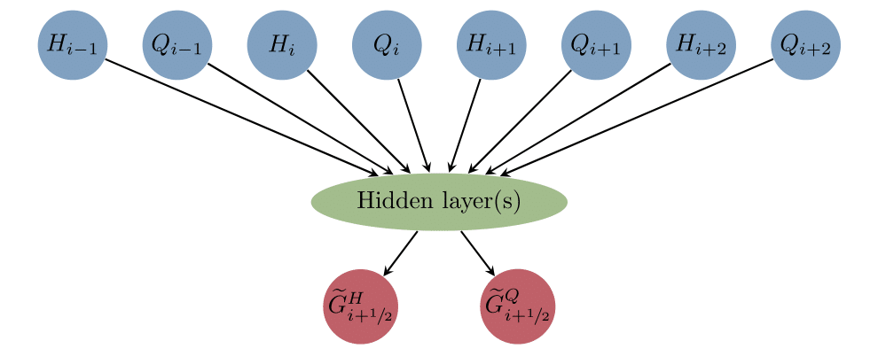
Figure 1: Schematic representation of the neural network used to approximate $G_{i+\nicefrac{{1}}{{2}}}=[G_{i+\nicefrac{{1}}{{2}}}^{H},G_{i+\nicefrac{{1}}{{2}}}^{Q}]$.

Figure 1 represents schematically the neural network used in our computations. The neural network has 3 hidden layers with 128 neurons each. We use the leaky ReLU [31] activation function $f(z)=\max\{\alpha z,z\}$ with $\alpha=0.01$. We also employ early stopping and data normalization as part of our regularization strategy. We use the default values of the NeuralNet class of the skorch package, unless stated otherwise. In particular, the default training algorithm torch.optim.SGD of the PyTorch package is used in our experiments.

For the training dataset, we generate $n$ trajectories of the SWE using random initial conditions

$$h_{0}(x)=\bar{H}+A_{h}\sin(2\pi k_{h}x/L+\phi_{h}),\quad v_{0}(x)=\bar{V}+A_{v}\sin(2\pi k_{v}x/L+\phi_{v}).$$ (15)

The constant average height $\bar{H}=2.0$ is used in all initial conditions. The remaining parameters are randomly generated following the distributions $\bar{V}\sim Unif(1,2)$, $A_{h},\,A_{v}\sim Unif(0.2,0.6)$, $k_{h},\,k_{v}\sim Unif\{1,6\}$, $\phi_{h},\,\phi_{v}\sim Unif(0,2\pi)$, where $Unif(a,b)$ denotes the continuous uniform distribution on $(a,b)$ and $Unif\{n,m\}$ represents the discrete uniform distribution between $n,m\in N$. We simulate each trajectory until $T^{train}$ and sample with the time step $\Delta t$. Specific values of $n$, $T^{train}$, and $\Delta t$ are listed in Section 4.

Next, we run coarse-mesh simulations and compute the “true” subgrid fluxes (11). In each time step, we generate $N_{c}$ subgrid fluxes $G_{i+\nicefrac{{1}}{{2}}}$, $i=1,\ldots,N_{c}$. This computation generates $N_{c}\times n\times T^{train}/\Delta t$ data points for training the neural network with the batch size of 128. Initially, we train for 500 epochs with a learning rate of $\gamma=0.1$. Subsequently, we continue training for further 2000 epochs with a lower learning rate of $\gamma=0.001$. As a regularization technique, we implement early stopping during both stages of training.

3.2 Flux Limiting

One of the major drawbacks of machine learning is that there is a considerable gap in the theoretical understanding of neural networks. In our context, neural networks are treated as “black box” generators of subgrid fluxes $\widetilde{G}_{i+\nicefrac{{1}}{{2}}}$. The addition of these fluxes to $\bar{F}_{i+\nicefrac{{1}}{{2}}}$ can produce spurious oscillations and/or non-physical numerical solutions (e.g., negative water heights). To address this issue, we integrate the monolithic convex limiting (MCL) procedure [22] into the flux-corrected coarse-mesh discretization

$$\frac{\mathrm{d}}{\mathrm{d}t}U_{i}=\frac{(\bar{F}_{i-\nicefrac{{1}}{{2}}}+\widetilde{G}_{i-\nicefrac{{1}}{{2}}}^{*})-(\bar{F}_{i+\nicefrac{{1}}{{2}}}+\widetilde{G}_{i+\nicefrac{{1}}{{2}}}^{*})}{\Delta X},$$ (16)

where $\widetilde{G}_{i\pm\nicefrac{{1}}{{2}}}^{*}$ denotes a constrained approximation to the network subgrid flux $\widetilde{G}_{i\pm\nicefrac{{1}}{{2}}}$. To explain the MCL design philosophy, we write (16) in the equivalent bar state form

$$\frac{\mathrm{d}}{\mathrm{d}t}U_{i}=\frac{1}{\Delta X}\bigl{[}\Lambda_{i-\nicefrac{{1}}{{2}}}(\bar{U}_{i-\nicefrac{{1}}{{2}}}^{*,+}-U_{i})+\Lambda_{i+\nicefrac{{1}}{{2}}}(\bar{U}_{i+\nicefrac{{1}}{{2}}}^{*,-}-U_{i})\bigr{]},$$ (17)

where $\Lambda_{i+\nicefrac{{1}}{{2}}}$ is the maximum wave speed depending on $U_{i}$ and $U_{i+1}$. The low-order LLF part of

$$\bar{U}_{i+\nicefrac{{1}}{{2}}}^{*,\pm}=\bar{U}_{i+\nicefrac{{1}}{{2}}}\pm\frac{\widetilde{G}_{i+\nicefrac{{1}}{{2}}}^{*}}{\Lambda_{i+\nicefrac{{1}}{{2}}}}$$ (18)

is given by

$$\bar{U}_{i+\nicefrac{{1}}{{2}}}:=\frac{U_{i+1}+U_{i}}{2}-\frac{1}{2\Lambda_{i+\nicefrac{{1}}{{2}}}}(f(U_{i+1})-f(U_{i})).$$ (19)

An invariant domain of a hyperbolic initial value problem is a convex admissible set containing all states that an exact solution may attain [16]. In the SWE context, a physical invariant domain $\mathcal{A}$ consists of all states $u=[h,hv]^{T}$ such that the water height $h$ is nonnegative. The bar state $\bar{U}_{i+\nicefrac{{1}}{{2}}}$ represents an averaged exact solution of the Riemann problem with the initial states $U_{i}$ and $U_{i+1}$ [16, 19]. Thus $\bar{U}_{i+\nicefrac{{1}}{{2}}}\in\mathcal{A}$ provided that $U_{i},U_{i+1}\in\mathcal{A}$. The MCL approach [17] ensures that $\bar{U}_{i\pm\nicefrac{{1}}{{2}}}^{*,\mp}\in\mathcal{A}$ whenever $\bar{U}_{i\pm\nicefrac{{1}}{{2}}}\in\mathcal{A}$. Each forward Euler stage of Heun’s method advances the given data in time as follows:

$$U_{i}^{\rm MCL}=U_{i}+\frac{\Delta T}{\Delta X}\bigl{[}\Lambda_{i-\nicefrac{{1}}{{2}}}(\bar{U}_{i-\nicefrac{{1}}{{2}}}^{*,+}-U_{i})+\Lambda_{i+\nicefrac{{1}}{{2}}}(\bar{U}_{i+\nicefrac{{1}}{{2}}}^{*,-}-U_{i})\bigr{]}.$$ (20)

If the time step $\Delta T$ satisfies the CFL condition

$$\frac{\Delta T}{\Delta X}[\Lambda_{i+\nicefrac{{1}}{{2}}}+\Lambda_{i-\nicefrac{{1}}{{2}}}]\leq 1,$$ (21)

then $U_{i}^{\rm MCL}$ is a convex combination of $U_{i}$ and $\bar{U}_{i\pm\nicefrac{{1}}{{2}}}^{*,\mp}$. It follows that (cf. [16])

$$U_{i},U_{i\pm 1}\in\mathcal{A}\quad\Rightarrow\quad U_{i},\bar{U}_{i\pm\nicefrac{{1}}{{2}}}\in\mathcal{A}\quad\Rightarrow\quad U_{i},\bar{U}_{i\pm\nicefrac{{1}}{{2}}}^{*,\mp}\in\mathcal{A}\quad\Rightarrow\quad U_{i}^{\rm MCL}\in\mathcal{A}.$$

Thus the MCL scheme is invariant domain preserving (positivity preserving) for time steps satisfying (21).

The above limiting strategy differs from classical flux-corrected transport (FCT) algorithms [9, 42] and their extensions to hyperbolic systems [15, 24, 30] in that it does not split the fully discrete scheme (20) into a low-order predictor step and an antidiffusive corrector step. Instead, inequality constraints are imposed on the intermediate states $\bar{U}_{i\pm\nicefrac{{1}}{{2}}}^{*,\mp}$ of the spatial semi-discretization. In addition to constraining them to stay in the set $\mathcal{A}$ of physically admissible states, the MCL procedure can be configured to enforce semi-discrete entropy inequalities and/or local maximum principles for scalar quantities of interest [23].

The sequential MCL algorithm for the SWE system [17, 18] imposes local bounds on $h$ and $v$. In the present paper, we use a one-dimensional finite volume version of this algorithm to limit the fluxes

$$\widetilde{G}_{i+\nicefrac{{1}}{{2}}}=[\widetilde{G}_{i+\nicefrac{{1}}{{2}}}^{h},\widetilde{G}_{i+\nicefrac{{1}}{{2}}}^{q}]^{T}.$$

By abuse of notation, individual components of coarse-mesh variables are denoted by lowercase letters in the remainder of this section. For example, $\bar{U}_{i+\nicefrac{{1}}{{2}}}=[\bar{h}_{i+\nicefrac{{1}}{{2}}},\bar{h}_{i+\nicefrac{{1}}{{2}}}\bar{v}_{i+\nicefrac{{1}}{{2}}}]^{T}$, where $\bar{v}_{i+\nicefrac{{1}}{{2}}}:={\bar{q}_{i+\nicefrac{{1}}{{2}}}}/{\bar{h}_{i+\nicefrac{{1}}{{2}}}}$. Let

$$h_{i}^{\min}:=\min(\bar{h}_{i-\nicefrac{{1}}{{2}}},\bar{h}_{i+\nicefrac{{1}}{{2}}}),\qquad h_{i}^{\max}:=\max(\bar{h}_{i-\nicefrac{{1}}{{2}}},\bar{h}_{i+\nicefrac{{1}}{{2}}}),$$ (22)

$$v_{i}^{\min}:=\min(\bar{v}_{i-\nicefrac{{1}}{{2}}},\bar{v}_{i+\nicefrac{{1}}{{2}}}),\qquad v_{i}^{\max}:=\max(\bar{v}_{i-\nicefrac{{1}}{{2}}},\bar{v}_{i+\nicefrac{{1}}{{2}}}).$$ (23)

Following Hajduk [17], we formulate local maximum principles for the limited bar states as follows:

$$h_{i}^{\min}\leq\bar{h}_{i+\nicefrac{{1}}{{2}}}^{*,-}\leq h_{i}^{\max},\qquad h_{i+1}^{\min}\leq\bar{h}_{i+\nicefrac{{1}}{{2}}}^{*,+}\leq h_{i+1}^{\max},$$ (24a)

$$\bar{h}_{i+\nicefrac{{1}}{{2}}}^{*,-}v_{i}^{\min}\leq\bar{q}_{i+\nicefrac{{1}}{{2}}}^{*,-}\leq\bar{h}_{i+\nicefrac{{1}}{{2}}}^{*,-}v_{i}^{\max},\qquad\bar{h}_{i+\nicefrac{{1}}{{2}}}^{*,+}v_{i+1}^{\min}\leq\bar{q}_{i+\nicefrac{{1}}{{2}}}^{*,+}\leq\bar{h}_{i+\nicefrac{{1}}{{2}}}^{*,+}v_{i+1}^{\max}.$$ (24b)

Since $\bar{h}_{i+\nicefrac{{1}}{{2}}}^{*,\pm}=\bar{h}_{i+\nicefrac{{1}}{{2}}}\pm\frac{\widetilde{G}_{i+\nicefrac{{1}}{{2}}}^{h,*}}{\Lambda_{i+\nicefrac{{1}}{{2}}}}$, the water height constraints (24a) are equivalent to

$$\Lambda_{i+\nicefrac{{1}}{{2}}}(\bar{h}_{i+\nicefrac{{1}}{{2}}}-h_{i}^{\max})\leq\widetilde{G}_{i+\nicefrac{{1}}{{2}}}^{h,*}\leq\Lambda_{i+\nicefrac{{1}}{{2}}}(\bar{h}_{i+\nicefrac{{1}}{{2}}}-h_{i}^{\min}),$$ (25)

$$\Lambda_{i+\nicefrac{{1}}{{2}}}(h_{i+1}^{\min}-\bar{h}_{i+\nicefrac{{1}}{{2}}})\leq\widetilde{G}_{i+\nicefrac{{1}}{{2}}}^{h,*}\leq\Lambda_{i+\nicefrac{{1}}{{2}}}(h_{i+1}^{\max}-\bar{h}_{i+\nicefrac{{1}}{{2}}}).$$ (26)

It follows that the best bound-preserving approximation to $\widetilde{G}_{i+\nicefrac{{1}}{{2}}}^{h}$ is defined by

$$\widetilde{G}_{i+\nicefrac{{1}}{{2}}}^{h,*}=\begin{cases}\min(\widetilde{G}_{i+\nicefrac{{1}}{{2}}}^{h},\Lambda_{i+\nicefrac{{1}}{{2}}}\min(\bar{h}_{i+\nicefrac{{1}}{{2}}}-h_{i}^{\min},h_{i+1}^{\max}-\bar{h}_{i+\nicefrac{{1}}{{2}}}))&\mbox{if}\ \widetilde{G}_{i+\nicefrac{{1}}{{2}}}^{h}\geq 0,\\ \max(\widetilde{G}_{i+\nicefrac{{1}}{{2}}}^{h},\Lambda_{i+\nicefrac{{1}}{{2}}}\max(\bar{h}_{i+\nicefrac{{1}}{{2}}}-h_{i}^{\max},h_{i+1}^{\min}-\bar{h}_{i+\nicefrac{{1}}{{2}}}))&\mbox{otherwise}.\end{cases}$$ (27)

To ensure the feasibility of the discharge constraints (24b), the bar state

$$\bar{q}_{i+\nicefrac{{1}}{{2}}}^{*,\pm}=\bar{q}_{i+\nicefrac{{1}}{{2}}}\pm\frac{\widetilde{G}_{i+\nicefrac{{1}}{{2}}}^{q,*}}{\Lambda_{i+\nicefrac{{1}}{{2}}}}=\bar{h}_{i+\nicefrac{{1}}{{2}}}^{*,\pm}\bar{v}_{i+\nicefrac{{1}}{{2}}}\pm\frac{\Delta\widetilde{G}_{i+\nicefrac{{1}}{{2}}}^{q,*}}{\Lambda_{i+\nicefrac{{1}}{{2}}}}$$

is defined using a limited counterpart $\Delta\widetilde{G}_{i+\nicefrac{{1}}{{2}}}^{q,*}=\widetilde{G}_{i+\nicefrac{{1}}{{2}}}^{q,*}-\widetilde{G}_{i+\nicefrac{{1}}{{2}}}^{h,*}\bar{v}_{i+\nicefrac{{1}}{{2}}}$ of the flux difference

$$\Delta\widetilde{G}_{i+\nicefrac{{1}}{{2}}}^{q}=\widetilde{G}_{i+\nicefrac{{1}}{{2}}}^{q}-\widetilde{G}_{i+\nicefrac{{1}}{{2}}}^{h,*}\bar{v}_{i+\nicefrac{{1}}{{2}}}.$$

The sequential MCL algorithm [17] calculates the limited differences $\Delta\widetilde{G}_{i+\nicefrac{{1}}{{2}}}^{q,*}$ and sets

$$\widetilde{G}_{i+\nicefrac{{1}}{{2}}}^{q,*}:=\widetilde{G}_{i+\nicefrac{{1}}{{2}}}^{h,*}\bar{v}_{i+\nicefrac{{1}}{{2}}}+\Delta\widetilde{G}_{i+\nicefrac{{1}}{{2}}}^{q,*}.$$ (28)

Similarly to the derivation of the water height limiter (27), we use the equivalent form

$$\Lambda_{i+\nicefrac{{1}}{{2}}}\bar{h}_{i+\nicefrac{{1}}{{2}}}^{*,-}(\bar{v}_{i+\nicefrac{{1}}{{2}}}-v_{i}^{\max})\leq\Delta\widetilde{G}_{i+\nicefrac{{1}}{{2}}}^{q,*}\leq\Lambda_{i+\nicefrac{{1}}{{2}}}\bar{h}_{i+\nicefrac{{1}}{{2}}}^{*,-}(\bar{v}_{i+\nicefrac{{1}}{{2}}}-v_{i}^{\min}),$$ (29)

$$\Lambda_{i+\nicefrac{{1}}{{2}}}\bar{h}_{i+\nicefrac{{1}}{{2}}}^{*,+}(v_{i+1}^{\min}-\bar{v}_{i+\nicefrac{{1}}{{2}}})\leq\Delta\widetilde{G}_{i+\nicefrac{{1}}{{2}}}^{q,*}\leq\Lambda_{i+\nicefrac{{1}}{{2}}}\bar{h}_{i+\nicefrac{{1}}{{2}}}^{*,+}(v_{i+1}^{\max}-\bar{v}_{i+\nicefrac{{1}}{{2}}})$$ (30)

of conditions (24b) to establish their validity for (28) with $\Delta\widetilde{G}_{i+\nicefrac{{1}}{{2}}}^{q,*}$ defined by

$$\Delta\widetilde{G}_{i+\nicefrac{{1}}{{2}}}^{q,*}=\begin{cases}\min(\Delta\widetilde{G}_{i+\nicefrac{{1}}{{2}}}^{q},\Lambda_{i+\nicefrac{{1}}{{2}}}\min(\bar{h}_{i+\nicefrac{{1}}{{2}}}^{*,-}(\bar{v}_{i+\nicefrac{{1}}{{2}}}-v_{i}^{\min}),\bar{h}_{i+\nicefrac{{1}}{{2}}}^{*,+}(v_{i+1}^{\max}-\bar{v}_{i+\nicefrac{{1}}{{2}}})))&\mbox{if}\ \Delta\widetilde{G}_{i+\nicefrac{{1}}{{2}}}^{q}\geq 0,\\ \max(\Delta\widetilde{G}_{i+\nicefrac{{1}}{{2}}}^{q},\Lambda_{i+\nicefrac{{1}}{{2}}}\max(\bar{h}_{i+\nicefrac{{1}}{{2}}}^{*,-}(\bar{v}_{i+\nicefrac{{1}}{{2}}}-v_{i}^{\max}),\bar{h}_{i+\nicefrac{{1}}{{2}}}^{*,+}(v_{i+1}^{\min}-\bar{v}_{i+\nicefrac{{1}}{{2}}})))&\mbox{otherwise}.\end{cases}$$ (31)

The enforcement of (24) guarantees positivity preservation and numerical admissibility of approximate solutions to the one-dimensional SWE system. For a more detailed description of the sequential MCL algorithm, we refer the interested reader to Schwarzmann [38]. Other examples of modern flux correction schemes for nonlinear hyperbolic systems and, in particular, for SWEs can be found in [5, 24, 29, 15, 34].

4 Numerical Results

Considerable effort has been made to develop NN-based numerical approximations that are consistent with the physics of underlying PDE models, but the analysis of the resulting numerical algorithms can be difficult. Thus, although deep learning has become extremely popular in the context of computational methods for PDEs, numerical schemes based on neural networks can produce non-physical solutions. In the approach that we proposed above, subgrid fluxes generated by a neural network are “controlled” by a mathematically rigorous flux limiting formalism. The main goal here is to demonstrate that flux limiting can improve the quality of a deficient subgrid model by eliminating non-physical oscillations.

In our fine-mesh simulations for the SWE system (2) with $g=9.812$, we discretize the computational domain $\Omega=(0,100)$ using $N_{f}=2000$ cells. As before, we assume that the fine-mesh discretization resolves all physical processes of interest properly. In particular, the numerical diffusion is negligible and further refinement does not produce any visible changes in the numerical solutions. We perform fine-mesh simulations using the time step $\Delta t=0.1\Delta x$. The IDP property of the LLF space discretization and the SSP property of Heun’s time-stepping method guarantee positivity preservation for this choice of $\Delta t$. Using the coarsening parameter $k=20$, we construct coarse-mesh discretizations with $N_{c}=100$ and $\Delta X=1$. The time step $\Delta T=0.005\Delta X$ of the reduced model is an integer multiple of $\Delta t$. Initial conditions for the testing dataset are generated using equation (15) with parameter values that are not present in the training dataset. Selected parameters of initial conditions used for testing are presented in Table 1. The software used in this paper is available on GitHub [37].

We tested many initial conditions in this study. The overall performance of our subgrid model is discussed at the end of this section. We refer to simulations on the fine mesh as full model experiments or DNS (Direct Numerical Simulation). The results of reduced model experiments are referred to as NN-reduced if no MCL flux correction is performed and as MCL-NN-reduced if the MCL fix is activated.

IC	$H_{0}$	$A_{h}$	$k_{h}$	$\varphi_{h}$	$V_{0}$	$A_{v}$	$k_{v}$	$\varphi_{v}$
1	2.0	0.2	3	0.0	1.0	0.0	0	0.0
2	2.0	0.45	4	2.78	1.1	0.5	3	4.5
3	2.0	0.45	4	2.78	1.1	0.5	4	4.5
4	2.0	0.2	3	0.0	1.1	0.1	2	0.0

Table 1: Parameters of initial conditions (15) used for testing.

A visual comparison of numerical solutions to the SWE obtained with $N_{f}=2000$ and $N_{c}=N_{f}/k$ confirms that the subgrid fluxes $G_{i+\nicefrac{{1}}{{2}}}$ are antidiffusive (not shown here; see [38]). Therefore, subgrid fluxes should “remove” additional diffusion resulting from the coarse-mesh discretization. However, this process is nonlinear and quite delicate. Since there is no control over the numerical performance of the neural network used to model subgrid fluxes, the NN-reduced model might produce non-physical solutions.

Several networks with the same configuration but with different amounts of training data are tested in this study. The amount of training data is determined by two parameters: (i) $n$, how many different trajectories are generated for training and (ii) $T^{train}$, the length of each trajectory. Each trajectory is sampled with the time step $\Delta t=0.1\Delta x$. Given a lot of training data, the network typically reproduces fluxes quite well and the reduced model performs much better. However, in practical situations, the amount of training data can be limited since it is impossible to know a priori how many trajectories need to be generated for training.

First, we present results for a relatively large amount of training data with $n=200$ and $T^{train}=80$. Figures 2 and 3 depict the discharge $q=hv$ and water height $h$ at time $t=200$ for several choices of initial conditions in simulations with the full model and both reduced models (without and with limiting).

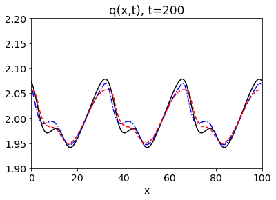
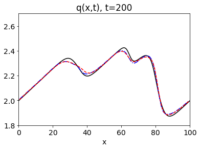
Figure 2: Discharge $q(x,t)=hv$ at time $t=200$ in simulations of the full model (black solid line) with $\Delta x=0.05$ and reduced models with $k=20$ ($\Delta x=1$) and NN trained with $n=200$ and $T=80$; Blue Dash-Dot Line - NN-reduced model, Red Dashed Line - MCL-NN-reduced model. Initial conditions with parameters in Table 1 (1 - top-left, 2 - top-right, 3 - bottom-left, 4 - bottom-right).

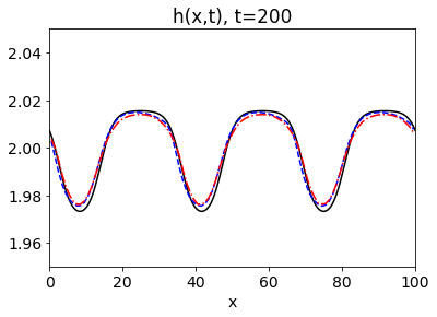
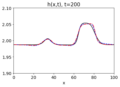
Figure 3: Water height $h(x,t)$ at time $t=200$ in simulations of the full model (black solid line) with $\Delta x=0.05$ and reduced models with $k=20$ ($\Delta x=1$) and NN trained with $n=200$ and $T=80$; Blue Dash-Dot Line - NN-reduced model, Red Dashed Line - MCL-NN-reduced model. Initial conditions with parameters in Table 1 (same location as in Figure 2).

In this example, the application of MCL to the subgrid fluxes does not significantly affect the quality of the results. It is worth pointing out that we test the performance of reduced models on a much longer interval compared to the length of training trajectories. Specifically, the length of the testing trajectory is $T^{test}=200$, while the length of each training trajectory is $T^{train}=80$. The performance of reduced models deteriorates for larger times and solutions with relatively small waves, but our ML reduced models can predict the dynamics of the SWE with larger waves for a much longer time. Numerical solutions for $T^{test}=400$ are compared in Figure 4.

Figure 4: Discharge $q(x,t)=hv$ at time $t=400$ in simulations of the full model (black solid line) with $\Delta x=0.05$ and reduced models with $k=20$ ($\Delta x=1$) and NN trained with $n=200$ and $T=80$; Blue Dash-Dot Line - NN-reduced model, Red Dashed Line - MCL-NN-reduced model. Initial conditions with parameters in Table 1 (same location as in Figure 2). Notice the difference in the vertical scale between the upper left subplot and the other three subplots.

The performance of ML reduced models changes drastically when the network is trained on a smaller dataset. For instance, we also generated the training dataset with $n=100$ and $T^{train}=40$. Thus, the training dataset is four times smaller compared to the training dataset for the reduced model used above. A comparison of the discharge at time $T=200$ for the DNS and simulations with the two reduced models (without and with the MCL fix) is presented in Figure 5. The reduced model without the limiter produces spurious oscillations in all four cases. These oscillations are particularly evident in the top-left subplot. The MCL-NN reduced model corrects these small-scale oscillations and produces physical solutions.

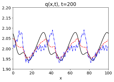
Figure 5: Discharge $q(x,t)=hv$ at time $t=200$ in simulations of the full model (black solid line) with $\Delta x=0.05$ and reduced models with $k=20$ ($\Delta x=1$) and NN trained with $n=100$ and $T^{train}=40$; Blue Dash-Dot Line - NN-reduced model, Red Dashed Line - MCL-NN-reduced model. Initial conditions with parameters in Table 1 (same location as in Figure 2).

One can use the MCL limiter as an indicator of the training quality for the NN reduced model. The MCL limiter is applied after training and the MCL-NN reduced model has approximately the same computational cost as the NN reduced model without the limiter. Therefore, if the two models produce very similar results, then this implies that the neural network approximates the fluxes with very good accuracy and is unlikely to produce non-physical solution values. However, if the two reduced models result in considerably different numerical solutions, then this can be an indicator that the neural network is not trained sufficiently well.

5 Conclusions

In this work, we developed a neural network reduced model for coarse-grained simulations using the shallow water equations. Starting with a fine-mesh finite-volume discretization, we defined the coarse-mesh variables as “box” spatial averages. Then all dynamic variables were decomposed into coarse-scale components (i.e., discretization of the SWE on a coarse mesh) and fine-scale fluctuations. The reduced model uses a relatively simple feed-forward neural network to represent flux corrections due to the subgrid terms (fluctuations).

The neural network is initially trained on a large dataset generated using direct numerical simulations with the fine-mesh discretization of the SWE. Our numerical studies indicate that the reduced model is capable of capturing the dynamics of coarse-scale variables for a wide range of initial conditions and for a much longer time compared with the simulation time of each trajectory in the training dataset. We would like to point out that the NN parameterization is local in space and requires only a four-point stencil. Local parameterizations have various practical advantages compared to global (e.g., Fourier space) parameterizations of unresolved degrees of freedom. For instance, our approach can be easily generalized to other types of boundary conditions and spatially non-homogeneous problems (e.g., with bottom topography). Moreover, in the spatially non-homogeneous case, neural networks can be trained in parallel using only local four-point stencil data. Finally, our neural network is relatively simple and has only three layers, thus, providing a minimal computational overhead. We will explore these issues in a subsequent paper for a more realistic ocean flow application.

The advantage of the approach considered here is that we train a reduced model for subgrid fluxes instead of estimating the whole right-hand side directly. Therefore, the reduced NN model is amenable to more traditional numerical techniques, such as flux limiting. Thus, we apply the Monolithic Convex Limiting (MCL) strategy to ensure that the machine learning component of the reduced model does not produce non-physical fluxes. Overall, we believe that combining machine learning with existing tools from numerical analysis has many potential advantages, such as improving the forecasting capabilities of ML reduced models, the ability to use simpler neural networks with smaller computational overhead, developing real-time and a posteriori tools for verifying the quality of ML reduced models.

Using numerical simulations, we demonstrated that the flux limiter plays a minimal role when the NN model is well trained. This is not surprising, since the Neural Network is capable of learning complex functions and, thus, is able to reproduce subgrid fluxes and ensure that they (almost) lie within physical limits. However, when the NN reduced model is not trained sufficiently well, the flux limiter plays a crucial role in suppressing non-physical oscillations. Moreover, the computational complexity of the NN- and MCL-NN reduced models is approximately the same since both of them are implemented on a coarse grid. Therefore, a detailed comparison of the numerical results generated by these two models can be used as an indicator of whether the machine-learning model is trained sufficiently well. Such an a posteriori test can then be used to assess the training quality of the neural network and make decisions regarding further training.

References

- [1] U. Achatz and G. Branstator, A two-layer model with empirical linear corrections and reduced order for studies of internal climate variability, J. Atmos. Sci., 56 (1999), pp. 3140–3160.
- [2] N. Agarwal, D. Kondrashov, P. Dueben, E. Ryzhov, and P. Berloff, A comparison of data-driven approaches to build low-dimensional ocean models, Journal of Advances in Modeling Earth Systems, 13 (2021), p. e2021MS002537.
- [3] J. Alcala and I. Timofeyev, Subgrid-scale parametrization of unresolved scales in forced Burgers equation using generative adversarial networks (GAN), Theoretical and Computational Fluid Dynamics, 35 (2021), pp. 875–894.
- [4] J. S. Alcala, Subgrid-scale parametrization of unresolved processes, PhD thesis, 2021.
- [5] P. Azerad, J.-L. Guermond, and B. Popov, Well-balanced second-order approximation of the shallow water equation with continuous finite elements, SIAM Journal on Numerical Analysis, 55 (2017), pp. 3203–3224.
- [6] J. Berner, U. Achatz, L. Batte, L. Bengtsson, A. de la Camara, H. M. Christensen, M. Colangeli, D. R. B. Coleman, D. Crommelin, S. I. Dolaptchiev, C. L. E. Franzke, P. Friederichs, P. Imkeller, H. Jarvinen, S. Juricke, V. Kitsios, F. Lott, V. Lucarini, S. Mahajan, T. N. Palmer, C. Penland, M. Sakradzija, J.-S. von Storch, A. Weisheimer, M. Weniger, P. D. Williams, and J.-I. Yano, Stochastic parameterization: Toward a new view of weather and climate models, Bulletin of the American Meteorological Society, 98 (01 Mar. 2017), pp. 565 – 588.
- [7] J. Berner, G. J. Shutts, M. Leutbecher, and T. N. Palmer, A spectral stochastic kinetic energy backscatter scheme and its impact on flow-dependent predictability in the ecmwf ensemble prediction system, Journal of the Atmospheric Sciences, 66 (2009), pp. 603 – 626.
- [8] T. Bolton and L. Zanna, Applications of deep learning to ocean data inference and subgrid parameterization, Journal of Advances in Modeling Earth Systems, 11 (2019), p. 376–399.
- [9] J. P. Boris and D. L. Book, Flux-corrected transport. I. SHASTA, a fluid transport algorithm that works, Journal of Computational Physics, 11 (1973), pp. 38–69.
- [10] S. I. Dolaptchiev, U. Achatz, and I. Timofeyev, Stochastic closure for local averages in the finite-difference discretization of the forced Burgers equation, Theor. Comput. Fluid Dyn., 27(3-4) (2013), pp. 297–317.
- [11] S. I. Dolaptchiev, I. Timofeyev, and U. Achatz, Subgrid-scale closure for the inviscid Burgers-Hopf equation, Comm. Math. Sci., 11(3) (2013), pp. 757–777.
- [12] M. Germano, U. Piomelli, P. Moin, and W. H. Cabot, A dynamic subgrid‐scale eddy viscosity model, Physics of Fluids A: Fluid Dynamics, 3 (1991), pp. 1760–1765.
- [13] S. Gottlieb, D. Ketcheson, and C.-W. Shu, Strong stability preserving Runge-Kutta and multistep time discretizations, World Scientific, 2011.
- [14] S. Gottlieb, C.-W. Shu, and E. Tadmor, Strong stability-preserving high-order time discretization methods, SIAM Review, 43 (2001), pp. 89–112.
- [15] J.-L. Guermond, M. Nazarov, B. Popov, and I. Tomas, Second-order invariant domain preserving approximation of the euler equations using convex limiting, SIAM Journal on Scientific Computing, 40 (2018), pp. A3211–A3239.
- [16] J.-L. Guermond and B. Popov, Invariant domains and first-order continuous finite element approximation for hyperbolic systems, SIAM Journal on Numerical Analysis, 54 (2016), pp. 2466–2489.
- [17] H. Hajduk, Algebraically constrained finite element methods for hyperbolic problems with applications in geophysics and gas dynamics, PhD thesis, Dortmund, Technische Universität, 2022.
- [18] H. Hajduk and D. Kuzmin, Bound-preserving and entropy-stable algebraic flux correction schemes for the shallow water equations with topography, ArXiv preprint, abs/2207.07261 (2022).
- [19] A. Harten, P. D. Lax, and B. van Leer, On upstream differencing and Godunov-type schemes for hyperbolic conservation laws, SIAM Review, 25 (1983), pp. 35–61.
- [20] D. D. Holm and B. T. Nadiga, Modeling mesoscale turbulence in the barotropic double-gyre circulation, Journal of Physical Oceanography, 33 (2003), pp. 2355–2365.
- [21] M. F. Jansen and I. M. Held, Parameterizing subgrid-scale eddy effects using energetically consistent backscatter, Ocean Modelling, 80 (2014), pp. 36–48.
- [22] D. Kuzmin, Monolithic convex limiting for continuous finite element discretizations of hyperbolic conservation laws, Computer Methods in Applied Mechanics and Engineering, 361 (2020), p. 112804.
- [23] D. Kuzmin and H. Hajduk, Property-Preserving Numerical Schemes for Conservation Laws, World Scientific, 2023.
- [24] D. Kuzmin, M. Möller, J. N. Shadid, and M. Shashkov, Failsafe flux limiting and constrained data projections for equations of gas dynamics, Journal of Computational Physics, 229 (2010), pp. 8766–8779.
- [25] C. Leith, Stochastic models of chaotic systems, Physica D: Nonlinear Phenomena, 98 (1996), pp. 481–491. Nonlinear Phenomena in Ocean Dynamics.
- [26] R. J. LeVeque, Finite volume methods for hyperbolic problems, vol. 31, Cambridge university press, 2002.
- [27] D. K. Lilly, A proposed modification of the Germano subgrid‐scale closure method, Physics of Fluids A: Fluid Dynamics, 4 (1992), pp. 633–635.
- [28] M. Lino, S. Fotiadis, A. A. Bharath, and C. D. Cantwell, Current and emerging deep-learning methods for the simulation of fluid dynamics, Proceedings of the Royal Society A: Mathematical, Physical and Engineering Sciences, 479 (2023), p. 20230058.
- [29] C. Lohmann and D. Kuzmin, Synchronized flux limiting for gas dynamics variables, Journal of Computational Physics, 326 (2016), pp. 973–990.
- [30] R. Löhner, K. Morgan, J. Peraire, and M. Vahdati, Finite element flux-corrected transport (fem–fct) for the euler and navier–stokes equations, International Journal for Numerical Methods in Fluids, 7 (1987), pp. 1093–1109.
- [31] A. L. Maas, A. Y. Hannun, A. Y. Ng, et al., Rectifier nonlinearities improve neural network acoustic models, in Proc. ICML, vol. 30, Atlanta, GA, 2013, p. 3.
- [32] A. J. Majda, I. Timofeyev, and E. Vanden-Eijnden, A mathematics framework for stochastic climate models, Comm. Pure Appl. Math., 54 (2001), pp. 891–974.
- [33] P. Moin, K. Squires, W. Cabot, and S. Lee, A dynamic subgrid-scale model for compressible turbulence and scalar transport, Physics of Fluids A: Fluid Dynamics, 3 (1991), pp. 2746–2757.
- [34] W. Pazner, Sparse invariant domain preserving discontinuous galerkin methods with subcell convex limiting, Computer Methods in Applied Mechanics and Engineering, 382 (2021), p. 113876.
- [35] V. Resseguier, M. Ladvig, and D. Heitz, Real-time estimation and prediction of unsteady flows using reduced-order models coupled with few measurements, Journal of Computational Physics, 471 (2022), p. 111631.
- [36] A. d. Saint-Venant et al., Theorie du mouvement non permanent des eaux, avec application aux crues des rivieres et a l’introduction de marees dans leurs lits, Comptes rendus des seances de l’Academie des Sciences, 36 (1871), pp. 174–154.
- [37] A. Schwarzmann, clf1: A collection of finite elements, finite volume, and machine learning solvers for one-dimensional conservation law problems; https://github.com/A-dot-S-dot/cls1.
- [38] A. Schwarzmann, Discrete model reduction for the shallow water equations using neural networks and flux limiting, Master’s thesis, TU Dortmund, 2023.
- [39] C.-W. Shu and S. Osher, Efficient implementation of essentially non-oscillatory shock-capturing schemes, Journal of Computational Physics, 77 (1988), pp. 439–471.
- [40] J. Smagorinsky, General circulation experiments with the primitive equations: I. the basic experiment, Monthly Weather Review, 91 (1963), pp. 99 – 164.
- [41] M. Zacharuk, S. I. Dolaptchiev, U. Achatz, and I. Timofeyev, Stochastic subgrid-scale parametrization for one-dimensional shallow-water dynamics using stochastic mode reduction, Quarterly Journal of the Royal Meteorological Society, 144 (2018), pp. 1975–1990.
- [42] S. T. Zalesak, Fully multidimensional flux-corrected transport algorithms for fluids, Journal of Computational Physics, 31 (1979), pp. 335–362.
- [43] C. Zhang, P. Perezhogin, C. Gultekin, A. Adcroft, C. Fernandez-Granda, and L. Zanna, Implementation and evaluation of a machine learned mesoscale eddy parameterization into a numerical ocean circulation model, Journal of Advances in Modeling Earth Systems, 15 (2023), p. e2023MS003697.