The Möbius Game: A Quantum-Inspired Test of General Relativity

Abstract

We present a tight inequality to test the dynamical nature of spacetime. A general-relativistic violation of that inequality certifies change of curvature, in the same sense as a quantum-mechanical violation of a Bell inequality certifies a source of entanglement. The inequality arises from a minimal generalization of the Bell setup. It represents a limit on the winning chance of a collaborative multi-agent game played on the Möbius graph. A long version of this Letter including other games and how these games certify the dynamical character of the celebrated quantum switch is accessible as arXiv:2309.15752 [gr-qc].

Einstein, Podolsky, and Rosen [1, 2] challenged the completeness of quantum theory. For a pair of spin-one-half particles in the singlet state $(\ket{\uparrow\downarrow}-\ket{\downarrow\uparrow})/\sqrt{2}$, it is possible to perfectly predict any spin component of one of them by interacting with its companion only—even if they are spacelike separated. But then, should not the spin components in complementary directions be encoded within each of the particles? Since the quantum-mechanical description fails to do so, is it possible to complete the theory with hidden variables? Bell [3], most strikingly, answered in the negative: The observations in any such theory are severely restricted compared to the quantum-mechanical capabilities. Suppose we distribute such a “hidden-variable” particle to an agent Alice, and another to a spacelike separated agent Bob. Then, we let each agent perform one out of two dichotomic measurements $X,Y\in\{0,1\}$ at random, and record the result $A,B\in\{0,1\}$. For this scenario, Bell’s theorem [4] states that their observations are bound by the “Bell inequality” $\Pr[A\oplus B=XY]\leq 3/4$ (the symbol $\oplus$ represents addition modulo two): The probability for coïnciding results iff at least one agent performed the $0$ measurement is limited by $3/4$. In stark contrast, if the agents were supplied with the quantum particles in the singlet state, then they may violate this inequality and satisfy the predicate with probability $(2+\sqrt{2})/4$ [5]: These “nonlocal” quantum-mechanical correlations are incompatible with local hidden-variable theories; the quantum-mechanical description of these spin particles cannot be completed.

Bell’s discovery is most fascinating not only for its foundational nature, but also for the device-independent methodology: Bell’s theorem is free of any technological, experimental, or theoretical specifications. Operations and agents, i.e., experimentalists, are employed as the units of the operational scientific practice drawing the attention into “doings or happenings rather than into objects or entities” [6]. Any observation that violates a “Bell inequality” disagrees with “local causality” [7]—the local creation and distribution of information (see, Ref. [8] for a breakdown of the assumptions needed for Bell’s theorem)—irrespective of how the observation came about. This, in fact, enables applications of highest practical relevance, e.g., the realization of cryptographic tasks without the necessity to trust the device manufacturer [9, 10]. Note that Bell’s theorem may be circumvented, e.g., with hidden variables delocalized in space or time [11, 12, 13, 14, 15].

(a)

(b)

Figure 1: (a) In the Bell setup, the agents are spacelike separated. Their observations may depend on some hidden variable generated withing their common past. (b) Here, the agents may be situated in any causal configuration, as long as the causal relations are not tampered with, and the agents may communicate accordingly.

Results.—In this Letter, we present device-independent tests for the dynamical nature of spacetime, i.e., whether relativistic correlations are incompatible with static causal order. Here, static causal order means that the causal relations are unaffected by the agents’ actions. This setup reflects a minimal generalization of Bell’s (see Fig. 1). We describe a relativistic setting within which any violation of the presented inequalities certifies the dynamical nature of the causal relations—the incompatibility with any static causal background. In general relativity, such a violation is best explained via change of curvature. This is analogous to the Bell case, where a quantum-mechanical violation of a Bell inequality indicates the presence of entanglement. The inequalities correspond to a limiting winning chance of collaborative multi-agent games played on directed graphs. The most promising game discovered is played on an orientation of the Möbius ladder (see Fig. 2). In contrast to other games uncovered in the longer version of this Letter [16], the Möbius game remains non-trivial for any number of agents.

The Möbius Game.— The game played on the oriented Möbius ladder is fairly simple. Each vertex on the directed graph represents an agent. A referee picks at random an arc $u\raisebox{2.15277pt}{ \leavevmode\hbox to10.5pt{\vbox to4.16pt{\text{[drawing]}}}}v$, a bit $x$, discloses the selected arc to all agents, and secretly communicates the bit $x$ to the agent $u$. The agents are said to win the game whenever agent $v$ guesses $x$. As we will show, the winning chance under static causal order is upper bounded by 11/12.

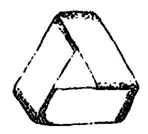
(a)

(b)

Figure 2: (a) Drawing of a Möbius strip (einseitiger Polyëder) by August Ferdinand Möbius [17, p. 520]. (b) The 7-Möbius digraph is an orientation of the Möbius ladder $M_{7}$.

Scenario.—Suppose a referee selects a “sender” $s$ and a distinct “receiver” $r$ from the set $[n]:=\{0,1,\dots,n-1\}$ of $n$ agents, and announces this selection $(s,r)$ to all agents. Moreover, the referee provides the “sender” with a bit $x$, and requests from the “receiver” a bit $a$. Thus, the input space of each agent is the set of distinct agent pairs $[n]^{2}\setminus\{(i,i)|i\in[n]\}$, and the “sender” has the additional input space $\{0,1\}$. Finally, the output space of the “receiver” is $\{0,1\}$, and all other agents are assumed to have a trivial output space $\{\bot\}$. The input-output behavior of this alliance is thus described by the conditional probability distribution $p(a|s,r,x)$.

Static Causal Order.—Upon reception of the input, each agent immediately responds with the output (which for all-but-one agent is trivial). We regard the realization of agent $i$’s output as the event $E_{i}$. Static causal order is now but a partial order $\sigma$ over the events $\{E_{i}\}_{i\in[n]}$, or, likewise, over $[n]$. We use $i\preceq_{\sigma}j$ to express that $E_{i}$ is in the causal past of $E_{j}$ with respect to the partial order $\sigma$, and $i\not\preceq_{\sigma}j$ for the alternative case. In the latter case, the output of agent $j$ cannot depend on the input to agent $i$. In the present scenario, the output $a$—which is produced by the “receiver”—is independent of the input $x$—which is provided to the “sender”—whenever $s\not\preceq_{\sigma}r$. In generality, the partial order $\sigma$ may be selected probabilistically. Thus, the input-output behavior $p(a|s,r,x)$ satisfies static causal order whenever it can be decomposed as a mixture of correlations that satisfy a partial order over the events, i.e., whenever there exists a distribution $p(\sigma)$ over partial orders, and a family of conditional probability distributions $\{p_{r,\sigma}^{\preceq}(a|s,r,x),p_{r,\sigma}^{\not\preceq}(a|s,r)\}_{r,\sigma}$, such that

$$\begin{split}p(a|s,r,x)&=\sum_{\sigma:s\preceq\sigma r}p(\sigma)p_{r,\sigma}^{\preceq}(a|s,r,x)\\ +&\quad\sum_{\sigma:s\not\preceq\sigma r}p(\sigma)p_{r,\sigma}^{\not\preceq r}(a|s,r)\,.\end{split}$$ (1)

Inequality.— The Möbius strip is the single-sided surface that is obtained by flipping one end of a strip and gluing it to the other end (see Fig. 2a). The corresponding graph is known as Möbius ladder $M_{k}$ [18], where one end of the $k$-ladder graph is crosswise connected to the other, i.e., it has the vertices $\{0,1\}\times[k]$, the “steps” $\{(0,i)\raisebox{2.15277pt}{ \leavevmode\hbox to9.34pt{\vbox to0.8pt{\text{[drawing]}}}}(1,i)|i\in[k]\}$, the “pole” edges $\{(\ell,i)\raisebox{2.15277pt}{ \leavevmode\hbox to9.34pt{\vbox to0.8pt{\text{[drawing]}}}}(\ell,i+1)|\ell\in\{0,1\},i\in[k-1]\}$, and the “crossings” $\{(0,k-1)\raisebox{2.15277pt}{ \leavevmode\hbox to9.34pt{\vbox to0.8pt{\text{[drawing]}}}}(1,0),(1,k-1)\raisebox{2.15277pt}{ \leavevmode\hbox to9.34pt{\vbox to0.8pt{\text{[drawing]}}}}(0,0)\}$. Here, we will consider the directed graph obtained by giving an orientation to each of the edges of the Möbius ladder. The $k$-Möbius digraph, which is defined for odd $k\geq 3$ only, is $M_{k}$ where the edge $(0,0)\raisebox{2.15277pt}{ \leavevmode\hbox to9.34pt{\vbox to0.8pt{\text{[drawing]}}}}(1,0)$ is oriented as $(0,0)\raisebox{2.15277pt}{ \leavevmode\hbox to9.34pt{\vbox to0.8pt{\text{[drawing]}}}}(1,0)$, and where each internal face of the ladder consistently forms a four cycle (see Fig. 2b). Also, we refer to any directed graph isomorphic to the $k$-Möbius digraph—regardless of the vertex names—as $k$-Möbius digraph. Note that this digraph has $3k$ arcs and that it is bipartite, i.e., two colors suffice to paint each of the vertices such that adjacent vertices have different colors.

Now, suppose $D=(\mathcal{V},\mathcal{A})$ is a $k$-Möbius digraph with vertices $\mathcal{V}\subseteq[n]$, arcs $\mathcal{A}$, and let $D^{\uparrow n}=([n],\mathcal{A})$ be $D$ where the vertex set is completed to $[n]$. Also, let $\mathcal{W}(D^{\uparrow n})$ be the event that the $n$ agents win the Möbius game when played on $D^{\uparrow n}$ with uniformly distributed inputs. Concretely, for some correlations $p(a|s,r,x)$, the winning chance is

$$\Pr[\mathcal{W}(D^{\uparrow n})]=\frac{1}{6k}\sum_{\begin{subarray}{c}x\in\{0,1\}\\ s\raisebox{1.20552pt}{ \leavevmode\hbox to7.09pt{\vbox to3.2pt{\text{[drawing]}}}}r\in\mathcal{A}\end{subarray}}p(x|s,r,x)\,.$$ (2)

Our main technical contribution is that if the $n$-agent-correlations $p(a|s,r,x)$, for any $n\geq 6$, satisfy static causal order, then this winning chance is bounded by $11/12$, or, more precisely, by

$$\Pr[\mathcal{W}(D^{\uparrow n})]\leq 1-\frac{k+1}{12k}\,.$$ (3)

This inequality is tight in the strongest sense: It defines a facet of the convex body of correlations $p(a|s,r,x)$ that satisfy static causal order. In the longer version of this Letter, we present further facet-defining inequalities for any number of agents $n\geq 2$.

Geometric Representation.—In a first part towards deriving the above inequality, we represent the set of correlations $p(a|s,r,x)$ that satisfy Eq. (1) geometrically. This is done by associating to each such conditional probability distribution the vector $\bm{p}:=(p(0|s,r,x))_{(s,r,x)}$. It is evident that the resulting body $\mathcal{P}_{n}\subseteq\mathbb{R}^{2n(n-1)}$ forms a convex polytope, i.e., it is the convex hull of a finite number of vectors, or, equivalently, it is the intersection of a finite number of halfspaces. The inequality (3) defines such a halfspace. In the next few paragraphs, we will derive that halfspace from the set $\operatorname{ext}(\mathcal{P}_{n})$ of extremal vectors of $\mathcal{P}_{n}$. We achieve this by first projecting the polytope to a lower-dimensional one $\mathcal{Q}_{n}$. As it turns out, the polytope $\mathcal{Q}_{n}$ is but the polytope of directed acyclic graphs (DAGs). Then, we recycle the facet-defining inequalities of $\mathcal{Q}_{n}$, which were derived in Ref. [19], and lift them to $\mathcal{P}_{n}$. The reader satisfied with that sketch and not looking for more details may safely skip to the section Relativity where we discuss the relativistic setup.

Properties.—The polytope $\mathcal{P}_{n}$ has three crucial properties: It is full-dimensional, all extremal points are deterministic, and it is what we call “pairwise centrally symmetric.” The first property states that the specification of the $2n(n-1)$ probabilities are necessary to identify $p(a|s,r,x)$ within $\mathcal{P}_{n}$. The second property states $\operatorname{ext}(\mathcal{P}_{n})\in\{0,1\}^{2n(n-1)}$. The third property is a specific form of central symmetry: If $\bm{p}=(\bm{p}_{0},\bm{p}_{1})$ is an extremal point, where we use $\bm{p}_{b}:=(p(0|s,r,b))_{(s,r)}$, then so is $(\bm{p}_{0}\oplus\bm{e}_{s^{\prime},r^{\prime}},\bm{p}_{1}\oplus\bm{e}_{s^{\prime},r^{\prime}})$ for any $s^{\prime},r^{\prime}$, where $\bm{e}_{s^{\prime},r^{\prime}}$ is the all-zero vector with a one in dimension $(s^{\prime},r^{\prime})$. To see this, consider the strategy that generates the former correlations, and modify it by letting the “receiver” flip the output bit upon input $s^{\prime},r^{\prime}$.

Projection.—We remove this symmetry of $\mathcal{P}_{n}$ with

$$\pi_{n}:\{0,1\}^{2d} \rightarrow\{0,1\}^{d}$$ (4)

$$(\bm{v}_{0},\bm{v}_{1}) \mapsto\bm{v}_{0}\oplus\bm{v}_{1}\,,$$ (5)

and define the resulting polytope $\mathcal{Q}_{n}$ through its extremal points $\operatorname{ext}(\mathcal{Q}_{n}):=\pi_{n(n-1)}(\operatorname{ext}(\mathcal{P}_{n}))$. The entry in dimension $(s,r)$ of some extremal $\bm{q}=\bm{p}_{0}\oplus\bm{p}_{1}$ is $p(0|s,r,0)\oplus p(0|s,r,1)$—it is zero if and only if the output $a$ of the “receiver” $r$ is independent of the input $x$ to the “sender” $s$. Thus, for each pair $(s,r)$, the vector $\bm{q}$ encodes the dependency of the output of the “receiver” from the input to the “sender.” Since each such $\bm{q}$ arises from a conditional probability distribution $p(a|s,r,x)$ satisfying Eq. (1), the dependencies must be compatible with a partial order of the agents. Moreover, since the “receiver” in any case may disregard the input to the “sender,” the dependencies encoded by $\bm{q}$ need not be transitive. Together this means that $\bm{q}$ is the adjacency vector of a DAG. Also note that each DAG over the vertices $[n]$ is represented as an extremal point of $\mathcal{Q}_{n}$. So, the polytope $\mathcal{Q}_{n}$ is but the polytope of DAGs.

The DAG Polytope.—In the context of discrete optimization, Grötschel, Jünger and Reinelt [19] uncovered some of the facet-defining inequalities of $\mathcal{Q}_{n}$. In particular, they show that for each $k$-Möbius digraph $D=(\mathcal{V}\subseteq[n],\mathcal{A})$, the inequality

$$\sum_{\begin{subarray}{c}u\raisebox{1.20552pt}{ \leavevmode\hbox to6.09pt{\vbox to0.4pt{\text{[drawing]}}}}v\in\mathcal{A}\end{subarray}}q_{u,v}\leq(5k-1)/2$$ (6)

is facet-defining for $\mathcal{Q}_{n}$: If some $\bm{q}=(q_{u,v})_{(u,v)}\in\mathbb{R}^{n(n-1)}$ violates that inequality, then $\bm{q}$ does not admit a decomposition into a convex combination of the adjacency vectors of DAGs.

Lifting Lemma.—We present the following lemma, which allows us to recycle the facets of $\mathcal{Q}_{n}$ as facets of $\mathcal{P}_{n}$. If the inequality $\sum_{i\neq j\in[n]}\chi_{i,j}q_{i,j}\leq c$ is facet-defining for $\mathcal{Q}_{n}$, non-negative, i.e., all coefficients $\chi_{(i,j)}$ are non-negative, and non-trivial, i.e., two or more coefficients are non-zero, then

$$\sum_{i\neq j\in[n]}\chi_{i,j}p_{i,j,0}-\sum_{i\neq j\in[n]}\chi_{i,j}p_{i,j,1}\leq c$$ (7)

is a non-trivial facet-defining inequality of $\mathcal{P}_{n}$, where $p_{i,j,b}$ is the entry in dimension $(i,j)$ of $\bm{p}_{b}$.

Our main technical contribution—the Möbius inequality (3)—is obtained by applying that Lifting Lemma (a proof of which is accessible in the longer version of the present letter [16]) to the Grötscherl-Jünger-Reinelt inequality (6). For a $k$-Möbius digraph $D=(\mathcal{V}\subseteq[n],\mathcal{A})$, we thus get

$$\sum_{i\raisebox{1.20552pt}{ \leavevmode\hbox to6.09pt{\vbox to0.4pt{\text{[drawing]}}}}j\in\mathcal{A}} p(0|i,j,0)-\sum_{i\raisebox{1.20552pt}{ \leavevmode\hbox to6.09pt{\vbox to0.4pt{\text{[drawing]}}}}j\in\mathcal{A}}p(0|i,j,1)$$ (8)

$$= \sum_{i\raisebox{1.20552pt}{ \leavevmode\hbox to6.09pt{\vbox to0.4pt{\text{[drawing]}}}}j\in\mathcal{A}}\left(p(0|i,j,0)-(1-p(1|i,j,1))\right)$$ (9)

$$= \sum_{\begin{subarray}{c}i\raisebox{1.20552pt}{ \leavevmode\hbox to6.09pt{\vbox to0.4pt{\text{[drawing]}}}}j\in\mathcal{A}\\ b\in\{0,1\}\end{subarray}}p(b|i,j,b)-|\mathcal{A}|\leq(5k-1)/2\,.$$ (10)

What remains, is to move $|\mathcal{A}|$ to the right-hand side, and to multiply the inequality with the uniform distribution of the referee announcing some $i\raisebox{2.15277pt}{ \leavevmode\hbox to9.34pt{\vbox to0.8pt{\text{[drawing]}}}}j$ and $x$, i.e., with $(2|\mathcal{A}|)^{-1}$.

Relativity.—In this section we adopt the Möbius game, as defined via the $k$-Möbius digraph $D=([k],\mathcal{A})$, to a relativistic setup in $1+1$ dimensions. Violations of the Möbius inequality in this setup certify the dynamical nature of spacetime. Note that if the events $\{E_{i}\}_{i\in[k]}$ are situated at distinct spacetime points in Minkowski spacetime, then it is impossible for the agents to violate the Möbius inequality: The events form a partial order. We will now generalize this setup to arrive at a description suitable for special as well as general relativity, where a special-relativistic violation remains impossible, and where a general-relativistic violation becomes feasible. First, it is not necessary for all events to be situated at distinct spacetime points. Because the $k$-Möbius digraph is bipartite, we may bipartition the nodes $[k]$ into two disjoint sets $\mathcal{V}_{L},\mathcal{V}_{R}$ according to the digraphs’ two-coloring. Events of the same “color” may be situated at the same location. Next, to get rid of absolute spacetime coordinates, we define the events as intersection of wordlines, as it is customary in general relativity. In fact, we define two non-overlapping spacetime regions $S_{L},S_{R}$, i.e., two non-overlapping causal diamonds, and position the events of each “color” in the respective region (see Fig. 3).

Figure 3: Two non-overlapping spacetime regions $S_{L},S_{R}$ that hold the respective events.

Any announced arc $s\raisebox{2.15277pt}{ \leavevmode\hbox to9.34pt{\vbox to0.8pt{\text{[drawing]}}}}r$ from the referee will never connect two events within the same region; the Möbius inequality cannot be violated in Minkowski spacetime.

We specify the setup further in order to enable possible general-relativistic violations of the inequality. Such violations may occur whenever the causal order of a pair of events is determined by an event in their common past. This, in principle, is possible by displacing matter in the common past. For that purpose, we add one agent without otherwise changing the graph ($n=k+1$), and locate the event of that additional agent in a spacetime region in the common past of $S_{L}$ and $S_{R}$. Also, we may regard $S_{L}$ and $S_{R}$ as spacelike separated. All-in-all, we end up with three spacetime regions in a causal configuration as displayed in Fig. 4.

Figure 4: Three non-overlapping spacetime regions are defined via intersections of past and future lightcones as constituted by the “announcers” $(\operatorname{An})$ and the “collectors” $(\operatorname{Co})$. The events of the agents $[k]=[n]\setminus\{n-1\}$ are partitioned according to their “color,” and happen in the regions $S_{L},S_{R}$ respectively. The event of the extra agent $n-1$ takes place in the common past within the region $S_{C}$.

Finally, we must ensure that the events take place within the prescribed regions, and that the agents receive their designated input from the referee. To achieve that, we split the referee into seven referees of two types, “announcer” ($\operatorname{An}$) and “collector” ($\operatorname{Co}$) who are initially positioned as shown in Fig. 4. As their names suggest, the “announcer” announce the inputs to the agents, and the “collectors” collect the outputs. The central “announcer” $\operatorname{An}_{C}$ shares a random bit $b_{L}$ ($b_{R}$) with the left (right) “announcer” $\operatorname{An}_{L}$ ($\operatorname{An}_{R}$), and broadcasts the arc $s\raisebox{2.15277pt}{ \leavevmode\hbox to9.34pt{\vbox to0.8pt{\text{[drawing]}}}}r\in\mathcal{A}$ together with the bit $x\oplus b_{\chi}$, where $\chi$ is the “color” of $s$. Both marginal “announcer” broadcast the shared bit $b_{L},b_{R}$. Therefore, the arc $s\raisebox{2.15277pt}{ \leavevmode\hbox to9.34pt{\vbox to0.8pt{\text{[drawing]}}}}r$ is accessible in the future light cone of the central announcer, i.e.,  $J^{+}(\operatorname{An}_{C})$. In contrast, if $s$ has “color” $\chi$, then the bit $x$ is accessible in $J^{+}(\operatorname{An}_{C})\cap J^{+}(\operatorname{An}_{\chi})$ only. The “collectors,” then again, travel at speed of light in the direction indicated. All agents of “color” $\chi$ must produce the output at the latest when $\operatorname{Co}^{\rightarrow}_{\chi}$ and $\operatorname{Co}^{\leftarrow}_{\chi}$ meet. Otherwise, the “collectors” abort the game. Our extra agent $n-1$ must produce the output at the latest when $\operatorname{Co}^{\rightarrow}_{R}$ and $\operatorname{Co}^{\leftarrow}_{L}$ meet. This ensures that the outputs are timely produced.

The rules described above, which are enforced by the referee, ensure that the events $\{E_{i}\}_{i\in\mathcal{V}_{\chi}}$ happen within the spacetime region

$$S_{\chi}:=J^{+}(\operatorname{An}_{C})\cap J^{+}(\operatorname{An}_{\chi})\setminus J^{+}(\operatorname{Co}^{\rightarrow}_{\chi})\cup J^{+}(\operatorname{Co}^{\leftarrow}_{\chi})\,,$$ (11)

and $E_{n-1}$ within $S_{C}:=J^{+}(\operatorname{An}_{C})\setminus J^{+}(Co^{\rightarrow}_{R})\cup J^{+}(Co^{\leftarrow}_{L})$. As described above, it is impossible to violate the Möbius inequality while respecting these rules of the game and without dynamically specifying the causal order in every round: Any theory with a static background must conform to the derived limits. In contrast, trespassing these limits might be possible in general relativity. Note that the setup described does not even allow the agents to saturate the Möbius inequality; the communicating agents are spacelike separated. The same reasoning as above, however, holds when $S_{L}$ and $S_{R}$ are timelike separated, as further outlined in the longer version of this Letter.

Conclusions and Open Questions.—A statistical violation of the presented inequalities, within the suggested setup, certifies the dynamical nature of spacetime, i.e., the absence of a static causal order. In relativity, this absence is best described by the backaction of matter on the spacetime manifold. In fact, a violation of the presented inequalities within the presented relativistic scenario is a signature for a change in curvature. A change of curvature, then again, requires the presence and dislocation of matter. Thus, a general-relativistic violation of the presented inequalities can also be regarded as a proof of the latter. One might speculate that the presented approach may also be used to detect gravitational waves.

Several open questions arise. More importantly, while we describe a relativistic setup to violate the Möbius inequality, an explicit description within the general-relativistic framework remains missing. Such a description may also shed light on the use of the inequality to detect gravitational waves. Theories with dynamical spacetime have a richer space of possible correlations. One might therefore wonder about their information-processing capabilities. Can we exploit these correlations to achieve tasks that are impossible in theories with a static background, analogous to the case of quantum information processing [20]? Does a dynamical spacetime allow for the implementation of cryptographic tasks that are otherwise impossible or not composable [21, 22]? On a technical side, one might wonder whether the Klein bottle, which is a generalization of the Möbius strip, also represents a facet of the polytope of correlations respecting static causal order.

Acknowledgments. We thank Luca Apadula, Flavio Del Santo, Andrea Di Biagio, and Stefan Wolf for helpful discussions. EET thanks Alexandra Elbakyan for providing access to the scientific literature. EET acknowledges support of the ID# 61466 and ID# 62312 grants from the John Templeton Foundation, as part of the “Quantum Information Structure of Spacetime (QISS)” project (qiss.fr), and support from the Research Network Quantum Aspects of Spacetime (TURIS). ÄB is supported by the Swiss National Science Foundation (SNF) through project 214808, and by the Hasler Foundation through project 24010.

References

Einstein et al. [1935]A. Einstein, B. Podolsky, and N. Rosen, Can quantum-mechanical description of physical reality be considered complete?, Physical Review 47, 777 (1935).
Bohm and Aharonov [1957]D. Bohm and Y. Aharonov, Discussion of experimental proof for the paradox of Einstein, Rosen, and Podolsky, Physical Review 108, 1070 (1957).
Clauser et al. [1969]J. F. Clauser, M. A. Horne, A. Shimony, and R. A. Holt, Proposed experiment to test local hidden-variable theories, Physical Review Letters 23, 880 (1969).
Bridgman [1956]P. W. Bridgman, Present state of operationalism, in The Validation of Scientific Theories (Beacon Press, Boston, 1956) pp. 74–79.
Bell [1990]J. S. Bell, La nouvelle cuisine, in Between Science and Technology, North-Holland Delta Series, edited by A. Sarlemijn and P. Kroes (Elsevier, Amsterdam, 1990) Chap. 6, pp. 97–115.
Wiseman and Cavalcanti [2017]H. M. Wiseman and E. G. Cavalcanti, Causarum investigatio and the two Bell’s theorems of John Bell, in Quantum [Un]Speakables II, The Frontiers Collection, edited by R. Bertlmann and A. Zeilinger (Springer International Publishing, Cham, 2017) Chap. 6, pp. 119–142.
Colbeck [2006]R. Colbeck, Quantum and relativistic protocols for secure multi-party computation, Ph.D. thesis, University of Cambridge (2006), arXiv:0911.3814 .
Price [1994]H. Price, A neglected route to realism about quantum mechanics, Mind 103, 303 (1994).
Baumeler et al. [2018]Ä. Baumeler, J. Degorre, and S. Wolf, Bell correlations and the common future, in Quantum Foundations, Probability and Information, edited by A. Khrennikov and B. Toni (Springer International Publishing, Cham, 2018) pp. 255–268.
Tselentis and Baumeler [2023]E.-E. Tselentis and Ä. Baumeler, The Möbius game and other Bell tests for relativity, arXiv:2309.15752 (2023), preprint.
Vilasini et al. [2019]V. Vilasini, C. Portmann, and L. del Rio, Composable security in relativistic quantum cryptography, New Journal of Physics 21, 043057 (2019).