KUNS-3010

Multi-Field Effects on Scalar Production in Stars

Yasuhiro Yamamoto¹ and Koichi Yoshioka²

¹Physics Division, National Center for Theoretical Sciences,
National Taiwan University, Taipei 10617, Taiwan
²Department of Physics, Kyoto University, Kyoto 606-8502, Japan

1 Introduction

In the realm of physics beyond the standard model, researchers have investigated various avenues, including the possibility of new types of particles, such as scalars and vectors. They have examined the number of these particles that might exist, their potential locations within the Universe, and the methods by which they could be detected. A significant area of inquiry is astrophysics, where stars serve as important testing grounds for new particle theories [1]. For example, the concept of using stars to study particles has proved to be of great assistance, such as in the case of axion [2, 3] which attempts to solve a puzzle called the strong CP problem [4], and as in the case of hidden photon [5, 6], a type of particle that can mix with the standard model photon. These hypothetical particles could be created inside stars through processes such as bremsstrahlung, where charged particles emit radiation as they interact. Attempts to detect these particles in stars have contributed to a refinement of our understanding of their properties and motivated experiments to detect them directly.

The CP-even scalar is another type of theoretical particle that may be created within stars through various processes. It often appears in theories that go beyond the standard model, such as those involving extended Higgs sectors or dark matter candidates [7, 8, 9]. In this paper, we study in detail the production of scalar particles in the medium. As a result of their electrically neutral composition, stars consist of multiple particles, including electrons, protons, neutrons, and atomic nuclei. It is commonly anticipated that the contributions to scalar production arise from a variety of particles with different masses, charges, and interactions with the scalar field. In general, the influence of heavier particles is expected to be limited and decoupled from the main physics. For example, in bremsstrahlung and Compton scattering, the scalar production is observed to decrease as the masses of heavier particles increase. Consequently, it is often assumed in discussions that only the contribution from the lightest particle (i.e., the electron) needs to be considered.

The present study examines the scalar production in the medium with a particular focus on the roles of particles other than electrons. While the impact of heavy particles only is indeed suppressed, it is possible for them to give a significant effect if combined with lighter particles (electrons). Depending on the particle energy and couplings, this combined effect could be substantial, potentially dominating the production process. Therefore, it is crucial to properly account for these characteristic effects in the medium. This type of phenomenon, such as the plasma mixing of CP-even scalars, leads to the screening and resonance effects of the production rate. It has been discussed in various contexts such as the production of dark photons [10, 11, 12], CP-even scalars [13, 14, 15], and axions in the presence of a magnetic field [16, 17, 18], imposing stringent constraints on model parameters. To fully understand these in-medium effects, it is necessary to evaluate the contributions from multiple fields, couplings, and various processes. While the effect of mixing and interference from heavy particles has not been seriously considered in previous literature, we demonstrate its importance by showing the significant impact on the scalar production rate.

The subsequent sections of the paper are structured as follows: In Section 2, we present the general expression for the scalar production rate, including its mixing with other particles. We explore how the scalar production process is influenced by the presence of various fields, couplings, and processes, especially in the context of mixing with longitudinal photons in the medium. Furthermore, we present a classification of these in-medium effect factors. Section 3 applies the multi-field behaviors to discuss the properties of scalar particles inferred from the stellar cooling processes in different scalar models. We highlight the distinct features observed in the parameter space due to the existence of in-medium effects. Finally, Section 4 summarizes our findings.

2 Scalar production in medium

Let us consider a scenario involving a scalar field $\phi$ (with mass $m_{\phi}$) that interacts through the CP-even Yukawa couplings with matter particles:

$${\cal L}\;=\;-y_{e}\phi\bar{e}e-y_{p}\phi\bar{p}p-y_{n}\phi\bar{n}n\,,$$ (2.1)

where $e$, $p$, and $n$ represent the Dirac fermions corresponding to the electron (with mass $m_{e}$ and charge $q_{e}=-e$), the proton (with charge $q_{p}=e$), and the neutron, respectively. For simplicity, the masses of the proton and the neutron are denoted by a common value $m_{N}$. It is also assumed that all particles are non-relativistic and non-degenerate.

As for heavy nuclei $X$ (with atomic number $Z_{X}$ and mass number $A_{X}$), it is assumed that their constituent nucleons can be treated coherently, given that typical temperatures are well below the binding energy of nuclei such as those found in stellar environments. Consequently, throughout this paper, we consider the mass of the nucleus to be $m_{X}=A_{X}m_{N}$, its charge to be $q_{X}=Z_{X}e$, and its coupling with the scalar field $\phi$ to be

$$y_{X}\,=\,Z_{X}y_{p}+(A_{X}-Z_{X})y_{n}\,.$$ (2.2)

2.1 Production rate

In the processes $X\to X^{\prime}+\phi$ and $X+\phi\to X^{\prime}$, the rates of production and absorption of the scalar $\phi$ are evaluated as

$$\Gamma_{\text{prod}} \,=\,\frac{1}{2\omega}\int\!d\Pi_{X,X^{\prime}}\,|\mathcal{M}_{X\to X^{\prime}\phi}|^{2}\,f_{X}(2\pi)^{4}\delta^{4}(k_{X}-k_{X^{\prime}}-k_{\phi})\,,$$ (2.3)

$$\Gamma_{\text{abs}}\, \,=\,\frac{1}{2\omega}\int\!d\Pi_{X,X^{\prime}}\,|\mathcal{M}_{X\phi\to X^{\prime}}|^{2}\,f_{X}(2\pi)^{4}\delta^{4}(k_{X}+k_{\phi}-k_{X^{\prime}})\,.$$ (2.4)

Here $X$ and $X^{\prime}$ are typically used to denote the sets of fields. The amplitude $\mathcal{M}$ in the vacuum is calculated within the framework of field theory. For the distribution function $f_{X}$ and the momenta $k_{X}$ and $k_{X^{\prime}}$, the summation is implied when multiple fields are involved in the initial and final states. The on-shell momentum of $\phi$ is $k_{\phi}=(\omega,\boldsymbol{k})$ (hereafter represented as $|\boldsymbol{k}|=k$). The damping rate, denoted by $\Gamma_{\phi}$, in the medium is given by $\Gamma_{\phi}=\sum(\Gamma_{\text{abs}}-\Gamma_{\text{prod}})$. According to thermal field theory [19, 20], it is related to the imaginary part of the in-medium self energy $\Pi_{\phi}$ as $\Gamma_{\phi}=-\text{Im}\,\Pi_{\phi}/\omega$ [21].

We focus on the scalar $\phi$ production, including the processes such as its generation via the mixing with photons in the medium. This type of production phenomenon has been explored for various bosons: the dark photon [10, 11], the CP-even scalar [13], and the axion in the presence of a background magnetic field [16, 17, 18]. These studies have imposed notable constraints on the properties of these bosons. If $\phi$ mixes with the longitudinal photon $\gamma_{L}$ (the plasmon), the resulting sum of all contributions through the mixing leads to the self energy,

$$\Pi_{\phi}\,=\,\Pi_{\phi\phi}-\frac{\Pi_{\phi L}\Pi_{L\phi}}{\Pi_{LL}-K^{2}}\,.$$ (2.5)

See Appendix A for the derivation. Here $\Pi_{XY}$ denotes the sum of all one-particle irreducible loop contributions to the $XY$ two-point functions, and $K$ is the (generally off-shell) four-momentum of external particles. By taking the imaginary parts of both sides of (2.5), we find the production rate can be rewritten as

$$\Gamma_{\text{prod}}\,=\,\frac{1}{2\omega}\!\int\!d\Pi_{X,X^{\prime}}\,|\mathcal{M}_{X\to X^{\prime}\phi}^{\text{eff}}|^{2}f_{X}(2\pi)^{4}\delta^{4}(k_{X}-k_{X^{\prime}}-k_{\phi})\,,$$ (2.6)

where the effective $\phi$ production amplitude in the medium is given by taking into account the mixing with plasmons,

$$\mathcal{M}_{X\to X^{\prime}\phi}^{\text{eff}}\,=\,\mathcal{M}_{X\to X^{\prime}\phi}\,-\,\frac{\Pi_{L\phi}}{\Pi_{LL}-K^{2}}\,\mathcal{M}_{X\to X^{\prime}L}\,.$$ (2.7)

The amplitude $\mathcal{M}_{X\to X^{\prime}L}$ represents the plasmon production for the same set of initial and final states ($X,\,X^{\prime}$). The plasmon momentum is taken to be $k_{L}=k_{\phi}$. According to this expression, the production rate in the medium can be obtained by replacing $\mathcal{M}_{X\to X^{\prime}\phi}$ with $\mathcal{M}_{X\to X^{\prime}\phi}^{\text{eff}}$ in the expression of the vacuum amplitude, i.e., the amplitude in the absence of the plasmon mixing. The absorption rate also receives a similar replacement due to the mixing as $\mathcal{M}_{X\phi\to X^{\prime}}^{\text{eff}}=\mathcal{M}_{X\phi\to X^{\prime}}-\Pi_{\phi L}/(\Pi_{LL}-K^{2})\mathcal{M}_{XL\to X^{\prime}}$.

2.2 In-medium effects

The effective production amplitude (2.7) in the medium can be expressed in the following form

$$|\mathcal{M}_{X\to X^{\prime}\phi}^{\text{eff}}|^{2}\,=\,z_{\phi}\,c_{\phi}^{XX^{\prime}}|\mathcal{M}_{X\to X^{\prime}\phi}|^{2}\,,$$ (2.8)

$$z_{\phi} \,=\,\bigg{|}\frac{K^{2}}{K^{2}-\Pi_{LL}}\bigg{|}^{2}\,,$$ (2.9)

$$c_{\phi}^{XX^{\prime}} \,=\,\Big{|}1+\frac{1}{K^{2}\,\mathcal{M}_{X\to X^{\prime}\phi}}\big{(}\Pi_{L\phi}\mathcal{M}_{X\to X^{\prime}L}-\Pi_{LL}\mathcal{M}_{X\to X^{\prime}\phi}\big{)}\Big{|}^{2}\,.$$ (2.10)

The amplitude is divided into two components: the vacuum amplitude in the absence of mixing and two types of in-medium effect factors, $z_{\phi}$ and $c_{\phi}^{XX^{\prime}}$. The superscripts of the multi-field effect $c_{\phi}^{XX^{\prime}}$ denote the fields appearing in the process. The factor $z_{\phi}$ commonly appears for all processes.

Firstly, $z_{\phi}$ represents the common medium effect in the presence of mixing with plasmons. By parameterizing $\Pi_{LL}$ with the renormalizing factor as $\text{Re}\,\Pi_{LL}=(K^{2}/\omega^{2})\omega_{p}^{2}$ and $\text{Im}\,\Pi_{LL}=-(K^{2}/\omega)\Gamma_{L}$ [11], $z_{\phi}$ becomes

$$z_{\phi}\,=\,\frac{\omega^{4}}{(\omega^{2}-\omega_{p}^{2})^{2}+\omega^{2}\Gamma_{L}^{2}}\,,$$ (2.11)

where $\omega_{p}$ denotes the plasma frequency in the medium, and $\Gamma_{L}$ corresponds to the damping rate of the plasmon. As can be seen from the expression of (2.11), $z_{\phi}$ emerges as a universal factor associated with any process, regardless of the specific properties of $\phi$ and its production processes. With regard to the energy dependence, $z_{\phi}$ is almost $1$ in the high-energy regime $\omega>\omega_{p}$ that indicates the suppression of plasmon effect. In the vicinity of the resonance at $\omega\sim\omega_{p}$, the localized amplification of $\phi$ production arises, potentially yielding the dominant contribution [13]. Conversely, in the low-energy regime where $\omega<\omega_{p}$, the suppression occurs with respect to $\omega$, resulting in the screening of $\phi$ processes [15]. Defining $\omega_{c}$ by $\omega_{c}\Gamma_{L}(\omega_{c})=\omega_{p}^{2}$, there exist two distinct regions of screening: $z_{\phi}\sim(\omega/\omega_{p})^{4}$ for $\omega>\omega_{c}$ and $z_{\phi}\sim(\omega/\Gamma_{L})^{2}$ for $\omega<\omega_{c}$.

The factor $c_{\phi}$ captures the influence of multiple fields/multiple couplings in the medium. As will be seen later, $c_{\phi}^{XX^{\prime}}=1$ for any $\phi$ process in the case of a single field/single coupling. This is because the second term in (2.10) cancels out and there is no medium effect attributed to $c_{\phi}$. In general, the value of $c_{\phi}$ varies depending on the $\phi$ processes. The second term in (2.10) inversely correlates with the energy $\omega$ and increases in the lower energy region compared to $\omega_{p}$, potentially becoming a significant factor. This behavior contrasts with that of $z_{\phi}$, which induces the screening of processes at low energy. In conclusion, according to (2.8), the production rate of the scalar $\phi$ in the medium can be expressed as the product of (the ubiquitous factor $z_{\phi}$) $\times$ (the variable factor $c_{\phi}$ for each process) $\times$ (the production rate in the vacuum).

2.2.1 single field/coupling : only $z_{\phi}$

We assume particles in the medium to be non-relativistic and non-degenerate. In this case, their couplings to $\phi$ via Yukawa coupling $y$ and to $A^{0}$ via electromagnetic coupling $q$ exhibit the same form at the leading order. Furthermore, we observe that $\Pi_{\phi L}$ satisfies $\Pi_{\phi L}=\varepsilon_{L\,\mu}\,\Pi_{\phi A}^{\mu}=(-\sqrt{K^{2}}/k)\Pi_{\phi A}^{0}$ through the Ward-Takahashi identity. Here $\varepsilon_{L}$ represents the polarization vector of the longitudinal mode, $\varepsilon_{L}(K)=\tfrac{1}{\sqrt{K^{2}}}(k,\omega\boldsymbol{k}/k)$. Consequently, the ratio of coupling strength between a certain $\phi$ process and its corresponding $\gamma_{L}$ process is generally given by $y/q_{L}$ where we define $q_{L}=(-\sqrt{K^{2}}/k)\,q$.

As the simplest case, we consider a charged field with a single Yukawa coupling $y$. This is analogous to the situation of low-temperature electrons in the medium. For the production process $X\to X^{\prime}+\phi\;(\gamma_{L})$ driven by the coupling $y$ ($q$), the amplitudes satisfy

$$\mathcal{M}_{X\to X^{\prime}\phi}\,:\,\mathcal{M}_{X\to X^{\prime}L}\;=\;y\,:\,q_{L}\,.$$ (2.12)

Moreover, given the presence of only one type of field and coupling, we observe that

$$\Pi_{L\phi}\,:\,\Pi_{LL}\;=\;y\,:\,q_{L}$$ (2.13)

as well. Consequently, as seen in (2.10), the factor $c_{\phi}^{XX^{\prime}}$ becomes equal to 1 in this case, regardless of the detail of processes such as $X$ and $X^{\prime}$. This is why $c_{\phi}$ is referred to as the multi-field effect. The cancellation of the second term in (2.10) indicates the existence of a field basis in which (non-relativistic) electrons and $\phi$ do not interact. By taking an appropriate linear combination of $\phi$ and the plasmon depending on the coupling ratio $y/q_{L}$, one can define a new basis where the scalar $\phi^{\prime}$ has no Yukawa coupling. Then the direct $\Pi_{\phi^{\prime}\phi^{\prime}}$ becomes suppressed and the scalar is only generated through the mass mixing with the plasmon. Note that such a coupling-dependent field redefinition is generally not useful in the case of multiple fields with non-uniform coupling ratios. This suggests a possibility of important effects beyond only $z_{\phi}$, as discussed in the subsequent section.

In the end, the production rate of $\phi$ for the case of a single field/coupling is obtained by the product of the medium effect $z_{\phi}$ and the production rate in the absence of mixing $\Gamma_{\text{prod}}^{(\text{no mix})}$. If $\Gamma_{\text{prod}}^{(\text{no mix})}$ correlates to the damping rate of plasmon $\Gamma_{L}$ according to the relation (2.12) as $\Gamma_{\text{prod}}^{(\text{no mix})}=(y/q_{L})^{2}\Gamma_{\gamma_{L}\;\text{prod}}=(y/q)^{2}(k^{2}/\omega^{2})\,f_{\gamma}\Gamma_{L}$, then the $\phi$ production rate takes the form

$$\Gamma_{\text{prod}}\,=\,\frac{y^{2}}{q^{2}}\,\frac{f_{\gamma}k^{2}\omega^{2}\Gamma_{L}}{(\omega^{2}-\omega_{p}^{2})^{2}+\omega^{2}\Gamma_{L}^{2}}\,,$$ (2.14)

which is the well-known expression [13] for the $\phi$ production in the medium. It should be noted that throughout this expression, the energy and momentum are with respect to $\phi$.

It is necessary to address several points. Firstly, if we consider $\Gamma_{L}$ to be the actual damping rate of plasmon, it should cover the contributions from all processes. However, not all of these processes necessarily follow (2.12). Secondly, when calculating the damping rate of plasmon, particularly in stellar environments, there exists a contribution from the electron-nucleon bremsstrahlung process. Even if only one charged field has the Yukawa coupling to $\phi$, the relation (2.13) is modified by the presence of multiple charged fields, e.g., the electron and the nucleons. In any case, the cancellation in $c_{\phi}$ discussed above does not occur, and it is likely that the in-medium effects extend beyond just $z_{\phi}$.

2.2.2 multiple fields/couplings : $z_{\phi}$ and $c_{\phi}$

As explained above, $z_{\phi}$ is the common factor that is independent of the production processes. In contrast, $c_{\phi}$ determines the specific characteristics of the production rate for each process. The evaluation of $c_{\phi}$ requires the evaluation of $\Pi_{L\phi}$, which can be challenging in the general case beyond the simple scenario with a single field/coupling. In the following discussion, we proceed under the assumption $\Pi_{L\phi}(K)=\Pi_{\phi L}(K)$. In this situation, for any $X$ and $X^{\prime}$, the phase of $\mathcal{M}_{X\to X^{\prime}\phi}$ is equal to that of $\mathcal{M}_{X\to X^{\prime}L}$ where the external $\phi$ line is replaced with $\gamma_{L}$. This enables us to express $\Pi_{L\phi}$ from the relations between the amplitudes.

Let us consider the situation where two types of charged fields are present in the medium: the electron $e$ with the charge $q_{e}$ and a single type of atomic nucleus $X$ with the charge $q_{X}$ and mass $m_{X}$. The number densities of these particles in the medium are denoted by $n_{e}$ and $n_{X}$, respectively. In the context of stellar environments, which will be the focus of subsequent section, we study the bremsstrahlung and Compton processes for the production of $\phi$. These processes can be classified as follows: (i) the emission from electrons: $e$-$e$ bremsstrahlung, $e\gamma$ Compton, etc., (ii) the emission from nuclei: $X$-$X$ bremsstrahlung, $X\gamma$ Compton, etc., and (iii) the emission from both electrons and nuclei $X$: $e$-$X$ bremsstrahlung, etc. Each of these processes exhibits distinct in-medium effects, reflecting the influence of multiple fields and couplings. While the medium effects of process (iii) can be derived by combining those of (i) and (ii), we here present the case of (iii) independently, since it serves as a representative production process. According to (2.10), we find the in-medium effect factors $c_{\phi}^{e}$, $c_{\phi}^{X}$, and $c_{\phi}^{eX}$ for the processes (i), (ii), and (iii) as follows,

$$c_{\phi}^{e} \,=\,\Big{|}\,1+\frac{1}{\omega^{2}}\,\frac{q_{e}y_{X}-q_{X}y_{e}}{y_{e}}\Big{[}\frac{q_{X}n_{X}}{m_{X}}-i\frac{q_{X}}{m_{X}^{2}}P_{X}+\frac{i}{m_{X}}\Big{(}\frac{q_{e}}{m_{e}}-\frac{q_{X}}{m_{X}}\Big{)}P_{eX}\Big{]}\,\Big{|}^{2}\,,$$ (2.15)

$$c_{\phi}^{X} \,=\,\Big{|}\,1-\frac{1}{\omega^{2}}\,\frac{q_{e}y_{X}-q_{X}y_{e}}{y_{X}}\Big{[}\frac{q_{e}n_{e}}{m_{e}}-i\frac{q_{e}}{m_{e}^{2}}P_{e}-\frac{i}{m_{e}}\Big{(}\frac{q_{e}}{m_{e}}-\frac{q_{X}}{m_{X}}\Big{)}P_{eX}\Big{]}\,\Big{|}^{2}\,,$$ (2.16)

$$c_{\phi}^{eX} =\,\Big{|}\,1+\frac{1}{\omega^{2}}\frac{q_{e}y_{X}-q_{X}y_{e}}{y_{e}m_{X}-y_{X}m_{e}}\Big{[}q_{e}n_{e}+q_{X}n_{X}-i\frac{q_{e}}{m_{e}}P_{e}-i\frac{q_{X}}{m_{X}}P_{X}\Big{]}\,\Big{|}^{2}\,.$$ (2.17)

The functions $P$’s are defined as

$$P_{i} \,=\,\frac{q_{i}^{4}n_{i}^{2}}{60\pi^{3/2}m_{i}^{1/2}}\,\frac{T^{1/2}J(\omega)}{f_{\phi}\omega^{2}}+\frac{q_{i}^{2}n_{i}k}{6\pi}\,,$$ (2.18)

$$P_{ij} \,=\,\frac{q_{i}^{2}q_{j}^{2}n_{i}n_{j}m_{i}^{1/2}m_{j}^{1/2}}{6\sqrt{2}\pi^{3/2}(m_{i}+m_{j})^{1/2}}\,\frac{I(\omega)}{f_{\phi}T^{1/2}\omega^{2}}\,,$$ (2.19)

where $T$ is the temperature in the medium. $P_{i}$ means the contribution from the $i$ field, while $P_{ij}$ represents the contributions related to the $i$-$j$ bremsstrahlung. These functions correspond to the imaginary parts of the in-medium self energies. The dimensionless functions $I(\omega)$ and $J(\omega)$ are given by

$$I(\omega) \,=\,\int^{\infty}_{\tfrac{m_{\phi}}{T}}du\int^{\infty}_{0}\!dv\int^{1}_{-1}\!dz\,\sqrt{uv}\,e^{-u}\,\frac{\delta(u-v-\omega/T)}{u+v-2\sqrt{uv}\,z}\,,$$ (2.20)

$$J(\omega) \,=\,\int^{\infty}_{\tfrac{m_{\phi}}{T}}du\int^{\infty}_{0}\!dv\int^{1}_{-1}\!dz\,\sqrt{uv}\,e^{-u}\,\delta(u-v-\omega/T)\frac{(u+v)^{2}+12uvz^{2}}{\big{[}(u+v)^{2}-4uvz^{2}\big{]}^{2}}$$

$$\hskip 99.58464pt\times\Big{[}\,3\big{[}(u+v)^{2}-4uvz^{2}\big{]}\Big{(}1-\frac{m_{\phi}^{2}}{\omega^{2}}\Big{)}+\frac{4\omega^{2}}{T^{2}}+\frac{m_{\phi}^{2}}{T^{2}}\,\Big{]}\,.$$ (2.21)

The comments on the in-medium factors (2.15)–(2.17) are in order:

(i) $c_{\phi}^{A}$ does not include the contribution from $P_{A}$ ($A=i,\,j,\>ij$). This is analogous to the case of a single field/coupling where self-contributions cancel out in the second term of $c_{\phi}$ (2.10). For example, if a process $A$ yields the most substantial contribution, the corresponding $P_{A}$ may naturally give a significant effect. However this large $P_{A}$ does not affect the in-medium factor $c_{\phi}^{A}$ for the process $A$ itself, while it has a large impact on processes other than $A$.

(ii) The real part of $c_{\phi}^{eX}$ (2.17) is determined by the sum of $q_{e}n_{e}$ and $q_{X}n_{X}$. In the environment consisting of two particles $e$ and $X$, this contribution is cancelled out to zero due to the condition of electrical neutrality. The cancellation occurs because, under the neutral condition in the medium, the self energies of non-relativistic particles can be written in the forms proportional to the dipole-like combinations of Yukawa and electromagnetic couplings, which is analogous to the case of bremsstrahlung amplitudes.

(iii) All multi-field effects are proportional to the combination of couplings in the form of $q_{e}y_{X}-q_{X}y_{e}$. In other words, the effects are manifest only through a conspiracy of two types of fields, and hence called as the multi-field effect. A charged field without Yukawa coupling to $\phi$ can contribute to $c_{\phi}$ (via other charged fields), while a neutral field with Yukawa coupling also contributes to $c_{\phi}$. Another important point is that multi-field effects are absent if the electromagnetic charge $q_{i}$ is universally proportional to $y_{i}$. For example, consider the presence of extra gauge bosons such as the dark photon with kinetic mixing to the standard model photon. In this case, the extra boson couplings $y_{i}$ satisfy the relation $y_{i}=(\text{const})q_{i}$, regardless of the type of charged fields. Analogous evaluation of the in-medium effect factors reveals that multi-field effects are absent for the extra boson production [13] (and also [22] for deviations from the universality). The vanishing of multi-field effects can also be understood from the field redefinition discussed in the previous section. In the presence of multiple fields, if the ratios $y_{i}/q_{i}$ have a common value (that is, $q_{i}y_{j}=q_{j}y_{i}$), all multi-field effects disappear through a certain redefinition with a single rotation angle which is determined by this ratio.

The plasmon damping rate and the plasma frequency are found to be

$$\Gamma_{L} \,=\,\frac{1}{\omega}\Big{(}\frac{q_{e}}{m_{e}}-\frac{q_{X}}{m_{X}}\Big{)}^{2}P_{eX}+\frac{q_{e}^{2}}{\omega m_{e}^{2}}P_{e}+\frac{q_{X}^{2}}{\omega m_{X}^{2}}P_{X}\,,$$ (2.22)

$$\omega_{p}^{2} \,=\,\frac{q_{e}^{2}n_{e}}{m_{e}}+\frac{q_{X}^{2}n_{X}}{m_{X}}\,.$$ (2.23)

Taking in mind the electrically neutral condition in the medium, the dominant contribution to $\omega_{p}$ is given by the electrons, while the contributions from other nuclei are always suppressed by the hierarchical mass ratio $m_{e}/m_{N}$. Nevertheless, it should be noted that even if the contribution of heavy particles is suppressed, it may still give a dominant physical effect in cases that the leading-order cancellation occurs, as described above.

2.3 Production rates with in-medium effects

We analyze the property of $\phi$ production rates, taking into account both of the in-medium effect factors $z_{\phi}$ and $c_{\phi}$. We focus on the case with two species of particles in the medium: the electron ($e$) and the hydrogen nucleus (H). As illustrative examples, we study three types of processes, $e$-$e$ bremsstrahlung, H-H bremsstrahlung, and $e$-H bremsstrahlung.

Figure 1 (the left panel) shows the typical in-medium factors $z_{\phi}$ and $c_{\phi}$. The medium environment, such as the temperature and the number density, is chosen to be $T=1$ keV and $n_{e}=10^{26}$ cm^-3 which are similar to the solar interior. The Yukawa couplings are set to be $y_{e}=10^{-9}$ and $y_{H}/m_{H}=2y_{e}/9m_{e}$. The latter follows the relation [23] consistent with the Higgs portal model. The overall magnitude of Yukawa couplings does not change the qualitative behavior of the lines. The scalar mass $m_{\phi}$ is assumed to be sufficiently small, rendering its effect negligible in the figure. For larger values of $m_{\phi}$ compared to the plasma frequency, all in-medium effects such as the resonance and the screening disappear. The following provides a brief elucidation of $z_{\phi}$ and the three types of multiple-field factors $c_{\phi}$:

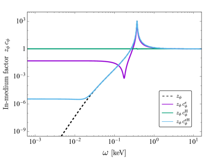
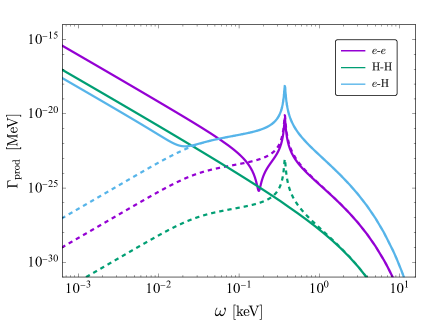
Figure 1: (Left) the in-medium effect factors $z_{\phi}$ and $c_{\phi}$. The purple, green, and blue lines correspond to the factors of $ee$ type, HH type, and $e$H type, respectively. The black dashed line represents $z_{\phi}$ alone. (Right) the production rates with the in-medium effect factors. Three types of bremsstrahlung are depicted: $e$-$e$ (purple), H-H (green), and $e$-H (blue). The temperature and the electron number density are set to the solar-like values, specifically $T=1$ keV and $n_{e}=10^{26}$ cm^-3. The Yukawa couplings are chosen to be $y_{e}=10^{-9}$ and $y_{H}/m_{H}=2y_{e}/9m_{e}$ as in the Higgs portal model. The qualitative behavior of the lines is independent of the overall magnitude of Yukawa couplings.

• The dashed black line, which partially overlaps with the blue line, illustrates $z_{\phi}$. The deviations from this dashed line indicate the effects of multiple fields and couplings, which are represented by $c_{\phi}$. As discussed in (2.11), the behavior of $z_{\phi}$ is characterized by the negligible effect ($z_{\phi}\simeq 1$) at high energy, the resonance ($z_{\phi}\gg 1$) near the plasma frequency $\omega_{p}$, and the screening ($z_{\phi}\ll 1$) at low energy. The behavior of $z_{\phi}$ remains almost unchanged even in the presence of multiple fields and couplings. As previously discussed, the plasma frequency is dominantly influenced by the lightest particle, the electron, regardless of the Yukawa couplings with $\phi$.

• For the $ee$ type (purple line), the impact of multi-field effects is negligible in the high-energy regime ($c_{\phi}^{e}\sim 1$). In the low-energy regime, however, the screening effect of $z_{\phi}$ is partially countered by $c_{\phi}^{e}$, leading to a deviation from the dashed black line. This weakening of the screening is attributable to the contributions from the real part of $c_{\phi}^{e}$ (2.15) for $\omega>\omega_{c}$ and to the contributions from the imaginary part of the $e$-H type process (the term $P_{eX}$) for $\omega<\omega_{c}$.

  Furthermore, in the $ee$ type, a dip-shaped feature is observed near the scale where the real part of $c_{\phi}^{e}$ (2.15) becomes zero. The location of this dip is approximately found to be $\omega\sim(y_{N}m_{e}/y_{e}m_{N})^{1/2}\omega_{p}$.

• For the HH type (green line), the influence of $z_{\phi}$ is entirely offset by $c_{\phi}$. This is due to the real part of $c_{\phi}$ for $\omega_{c}\lesssim\omega\lesssim\omega_{p}$ and the imaginary part for $\omega\lesssim\omega_{c}$. Consequently, $z_{\phi}c_{\phi}\simeq 1$ holds over the entire energy range, which eliminates the medium effects including the characteristic behaviors of resonance and screening. Thus the $\phi$ production amplitude is identical to that in the vacuum. This is mainly due to the fact that the plasma frequency is determined by the electron contribution and with no significant effect from other nuclei. The conclusion does not depend on the magnitude of hydrogen Yukawa coupling $y_{\text{H}}$ as long as $y_{\text{H}}\gtrsim y_{e}$.

• For the $e$H type (blue line), in the high-energy regime above $\omega_{c}$, the influence of multiple fields is absent and the medium effect is solely determined by $z_{\phi}$. Consequently, the resonance and screening of production rates appear. Below $\omega_{c}$, the cancellation of screening takes place due to the multi-field effect $c_{\phi}$, resulting in a constant medium factor. A weaker cancellation compared to the $ee$ and HH types can be explained by the self-cancellation within $c_{\phi}$, as previously discussed. Among the three bremsstrahlung processes under consideration, the $e$H type has the largest amplitude in the vacuum due to the hierarchical mass ratio $m_{e}/m_{\text{H}}$ and the Pauli blocking, which in turn makes it the weakest in the medium through the multi-field effect. The cancellation of screening in the $e$H type is attributed to the contribution of $ee$ bremsstrahlung. As a result, the blue line shows the suppression of approximately $(T/m_{e})^{2}\sim 10^{-5}$ compared to the cancellation observed in the $ee$ type (the terminal value of the purple line).

We further comment that there is little variation in $z_{\phi}$ and $c_{\phi}$ as a result of differences in medium properties. The only somewhat visible modification involves the shift in the plasma frequency (the location of resonance) and the temperature-dependent cancellation in the $e$-H bremsstrahlung. The other dependencies, such as those on Yukawa couplings and the species of nuclei, can be derived from the general expression (2.15)–(2.17).

The right panel of Figure 1 shows the $\phi$ production rates including the in-medium factors. Three types of production processes, the $e$-$e$, H-H, $e$-H bremsstrahlung, are represented by the purple, green, and blue lines, respectively. Based on the kinetic theory, i.e., without the medium effects, the production rate is known to simply behave as $\omega^{-3}$. In addition to this monotonic behavior, the inclusion of the universal factor $z_{\phi}$ only is shown by the dashed line for each color, exhibiting the resonance and screening phenomena [13, 15]. The additional inclusion of the multi-field factor $c_{\phi}$ yields the solid line for each color. The behavior of the production rate in the medium is thus determined by the product of $z_{\phi}\times c_{\phi}\times\text{(the monotonic behavior of kinetic theory)}$, and reflects the characteristics of $z_{\phi}$ and $c_{\phi}$ discussed above.

For example, the H-H bremsstrahlung process shows the identical behavior in the medium and in the vacuum, which matches to the kinetic theory result and unaffected by the resonance or screening effect. Furthermore, one can see the low-energy screening effect is cancelled for any process, thereby restoring the energy dependence in the vacuum. The low-energy values of production rates vary for each process due to the differences in the extent of screening cancellation. For example, the $e$-H bremsstrahlung, which has the largest rate in the vacuum, experiences the weakest cancellation and then the $e$-$e$ bremsstrahlung becomes the dominant production rate at lower energy. Consequently, in terms of the production number, the $e$-$e$ bremsstrahlung may exceed the resonance. (If the absorption of $\phi$ in the medium is taken into account, the production rate saturates at the energy where the rate is roughly equal to typical medium size.)  It is also mentioned that as the resonance is universally governed by $z_{\phi}$, the most significant bremsstrahlung process in the vacuum, i.e., the $e$-H one, also dominantly contributes to the resonance.

3 Stellar cooling

The existence of extra particles interacting with the standard model fields, such as a new scalar and an extra photon, results in the emission of these particles which serve as additional sources of energy loss. This phenomenon is observed in astrophysical objects, which provides various constraints on the property of these extra particles [1]. In the following, we will discuss the constraints on the CP-even scalar $\phi$ obtained from the stellar cooling argument, with particular focus on the Sun and horizontal-branch (HB) stars. So far, various single-field analyses have been performed in previous literature, see for example [13, 14, 24, 25]. In the medium of stars, the total electric charge should be neutral in the presence of electrons and nucleons as well as atomic nuclei formed by their accumulation. When the CP-even scalar $\phi$ couples to these multiple fields with different charges, masses, and couplings, the stellar cooling via the $\phi$ emission can be evaluated by using the results in the previous section.

3.1 Cooling processes and emission rates

In this work, we suppose that the Sun is composed of electrons, hydrogen, and helium. The HB stars are similarly assumed to be composed of electrons and helium for simplicity. We present several specific expressions of the production rates for electrons and helium (corresponding to the HB stars), while the production rates involving multiple species of nuclei (like the Sun) are given in Appendix B.

When the scalar $\phi$ generally has the Yukawa couplings to electrons and nucleons as in the Lagrangian (2.1), the following $\phi$ production processes can be effective at the energy scale in stars (now HB stars): (i) $e$-$e$ bremsstrahlung : $e+e\to e+e+\phi$,  (ii) He-He bremsstrahlung : $\text{He}+\text{He}\to\text{He}+\text{He}+\phi$,  (iii) $e$-He bremsstrahlung : $e+\text{He}\to e+\text{He}+\phi$,  (iv) $e$ Compton-like : $e+\gamma\to e+\phi$, and (v) He Compton-like : $\text{He}+\gamma\to\text{He}+\phi$. The processes (i) and (ii) receive the suppression of $T/\text{mass}$ compared to (iii) due to the cancellation resulting from the existence of identical particles in the final states. We nevertheless include them since they can still be dominant processes in some case, as demonstrated by the multi-field effects discussed in the previous section. The above bremsstrahlung processes are all photon-mediated. In the process (ii), there is also the pion-mediated one, which is not included because of its suppression by $(T/m_{N})^{2}$ compared to the photon-mediated CP-even scalar production. Moreover, the emission of $\phi$ from the mediator photon can also be neglected as being small. For example, when the coupling between $\phi$ and $\gamma$ is induced by standard-model fermion loops, the ratio of production rates is approximately ($\gamma$ emit)/($e$ emit) $\sim(T/m_{e})(\alpha/4\pi)^{2}\ll 1$.

Assuming non-relativistic electrons and nucleons, the production rates for these processes including the full in-medium effects are found to be

$$\Gamma_{\text{prod}}^{ee} \,=\,z_{\phi}c_{\phi}^{e}\frac{e^{4}y_{e}^{2}n_{e}^{2}T^{1/2}k^{2}J(\omega)}{60\pi^{3/2}m_{e}^{5/2}\omega^{5}}\,,$$ (3.1)

$$\Gamma_{\text{prod}}^{\text{HeHe}} \,=\,z_{\phi}c_{\phi}^{\text{He}}\frac{2e^{4}y_{N}^{2}n_{\text{He}}^{2}T^{1/2}k^{2}J(\omega)}{15\pi^{3/2}m_{N}^{5/2}\omega^{5}}\,,$$ (3.2)

$$\Gamma_{\text{prod}}^{e\text{He}} \,=\,z_{\phi}c_{\phi}^{e\text{He}}\frac{\sqrt{2}e^{4}n_{e}n_{\text{He}}m_{e}^{1/2}}{3\pi^{3/2}}\Big{(}\frac{y_{e}}{m_{e}}-\frac{y_{N}}{m_{N}}\Big{)}^{2}\frac{k^{2}I(\omega)}{T^{1/2}\omega^{5}}\,,$$ (3.3)

$$\Gamma_{\text{prod}}^{e\gamma} \,=\,z_{\phi}c_{\phi}^{e}\frac{e^{2}y_{e}^{2}n_{e}f_{\phi}k^{3}}{6\pi m_{e}^{2}\omega^{3}}\,,$$ (3.4)

$$\Gamma_{\text{prod}}^{\text{He}\gamma} \,=\,z_{\phi}c_{\phi}^{\text{He}}\frac{2e^{2}y_{N}^{2}n_{\text{He}}f_{\phi}k^{3}}{3\pi m_{N}^{2}\omega^{3}}\,.$$ (3.5)

The medium effect $z_{\phi}$ is given by (2.11), and $c_{\phi}$’s and the plasma frequency are obtained by substituting the masses and coupling constants in (2.15)–(2.17), (2.23) by those of electron and helium $q_{e}=-e$, $q_{\text{He}}=2e$, $m_{\text{He}}=4m_{N}$, and $y_{\text{He}}=2y_{p}+2y_{n}\equiv 4y_{N}$. In HB stars with the composition ratio assumed above, the number density satisfies $n_{\text{He}}=n_{e}/2$ according to the condition of electrical neutrality, and hence the real part of $c_{\phi}^{e\text{He}}$ cancels out. In the above production rates, the contributions of heavy nuclei enter via the Yukawa couplings $y_{p,n}$ and are suppressed by the nucleon mass, with the suppression factor being $y_{p,n}/m_{N}$. In the case of a scalar coupled to the standard model through the mixing with the Higgs boson, referred to as the Higgs portal scalar in the following, the Yukawa coupling is generally proportional to the corresponding mass. Consequently, the contribution of heavy nuclei is not negligible since $y_{X}/m_{X}\sim y_{p,n}/m_{N}\sim y_{e}/m_{e}$. Furthermore, the effects of heavy nuclei are also observed through the multi-field effects $c_{\phi}$. These effects can give characteristic influences on the scalar production as previously discussed.

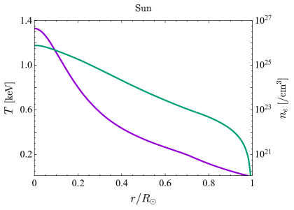
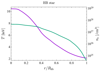
Figure 2: Typical profiles of the temperature (purple line) and the electron number density (green line) inside stars: (left) the Sun [26, 22] and (right) HB stars (data taken from [1]). The solar radius is $R_{\odot}=7\times 10^{10}$ cm. For HB stars, we here choose the radius as $R_{\text{hb}}=5.4\times 10^{9}$ cm within which the helium processes are important.

The energy emission rate per unit time from stars is evaluated by

$$Q^{i}\,=\,\int\!d^{3}\boldsymbol{r}\!\int\!\frac{d^{3}\boldsymbol{k}}{(2\pi)^{3}}\,\omega\,\Gamma_{\text{prod}}^{i}\,=\,\frac{1}{2\pi^{2}}\!\int_{0}^{R}\!\!dr\,r^{2}\!\int\!d^{3}\boldsymbol{k}\,\omega\,\Gamma_{\text{prod}}^{i}(T(r),n(r))$$ (3.6)

for each process. We assume the internal structure of stars to be spherically symmetric. Here $r$ and $R$ represent the distance from the center and the radius of a star, respectively. In the above expression, the opacity factor denoting the scalar absorption in the medium has been dropped, as this has no significant effect in the parameter regions of interest. The profiles of the temperature $T(r)$ and the electron number density $n_{e}(r)$ for the Sun and HB stars are shown in Figure 2. As a simplified model for evaluating the energy emission rate, the Sun is assumed to have the mass composition of hydrogen and helium with the ratio of $3:1$, and HB stars are considered to consist solely of helium. In HB stars, depending on the degree of evolution, carbon and oxygen may also be present in the core, but we neglect their effects for simplicity of calculation. While there is also the region of hydrogen burning outside the helium-dominated portion (referred to in Figure 2 as within the radius $R_{\text{hb}}=5.4\times 10^{9}$ cm), the effect there on the stellar energy loss through $\phi$ emission is negligible due to the low number density.

The emission rate (3.6) is generally evaluated by using the profiles. Here we adopt a convenient prescription for quantitative evaluation [25] where certain uniform temperature $T_{*}$ and density $n_{*}$ can mimic the evaluation using the profiles. There are three types of energy emission processes: the A-B bremsstrahlung, the A-A bremsstrahlung, and the A-$\gamma$ Compton-like (A, B = electron, nucleus). For these processes, we show in Figure 3 the uniform temperature and density at which the emission rates match to (3.6) using the profiles given in Figure 2.

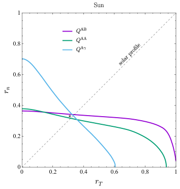
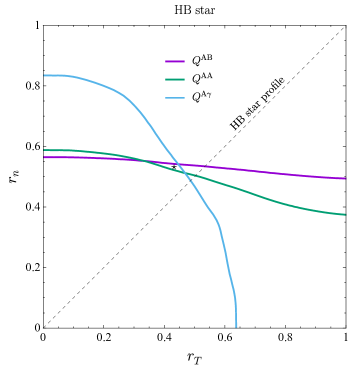
Figure 3: Uniform temperature and density capturing the energy emission rates using the profiles of Figure 2. The horizontal and vertical axes correspond to the temperature $T(r_{T}R)$ and the density $n_{i}(r_{n}R)$, respectively, where $R$ is the radius of each star. The purple, green, and blue lines means the comparisons with the A-B type bremsstrahlung, the A-A type bremsstrahlung, and the A-$\gamma$ Compton-like processes, respectively. (left) the Sun and (right) HB stars. The black stars correspond to $T_{*}=0.56$ keV and $n_{e*}=4.6\times 10^{24}$ cm^-3 on the left, and $T_{*}=6$ keV and $n_{e*}=1.1\times 10^{27}$ cm^-3 on the right.

The uniform temperature $T_{*}$ and density $n_{e*}$ are parameterized by $r_{T}$ and $r_{n}$ using the profile functions such that $T_{*}=T(r_{T}R)$ and $n_{*}=n(r_{n}R)$ where $R$ is the radius of each star. The left panel corresponds to the Sun, while the right panel shows the results for HB stars. It is found in both cases that the lines for three types of processes nearly coincide at a single point. That indicates the evaluation using the profile can be reproduced by the uniform temperature and density. In the following numerical analysis, we adopt this prescription and use the uniform temperature and density marked with the black stars in Figure 3, which specifically correspond to

   Sun : $$\quad T_{*}\,=\,0.56~{}\text{keV}\,,\qquad n_{e*}\,=\,4.6\times 10^{24}~{}\text{cm}^{-3}\,,$$ (3.7)

HB star : $$\quad T_{*}\,=\,6~{}\text{keV}\,, n_{e*}\,=\,1.1\times 10^{27}~{}\text{cm}^{-3}\,.$$ (3.8)

3.2 Leptonic/hadronic couplings

Consider the case that the scalar $\phi$ has Yukawa couplings both to the electrons and nucleons. In the stellar medium, both the electrons and nuclei are present, capable of producing $\phi$ and emitting the stellar energy. The Yukawa coupling with nucleons is considered isoscalar, which means it is common both to the protons and neutrons. Consequently, the Yukawa coupling with the nucleus $X$ is given by $y_{X}=A_{X}y_{N}$, $A_{X}$ being the mass number of $X$. The present model parameters then consist of two Yukawa couplings, one for leptonic and one for hadronic interactions, $y_{e}$ and $y_{N}$, respectively. By comparing the production of a hypothetical scalar $\phi$ with the observational data, the limits on these couplings can be discussed in the context of stellar cooling. In the analysis of this subsection, we set the scalar mass to a typical value of $m_{\phi}=10^{-2}$ keV.

The bounds on the leptonic/hadronic scalar couplings resulting from stellar cooling are illustrated in Figure 4.

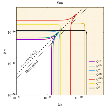
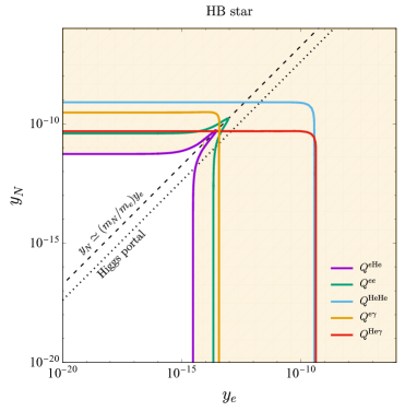
Figure 4: The bounds on scalar leptonic/hadronic Yukawa couplings from the stellar cooling. (left) the Sun and (right) HB stars. The orange shaded area represents the excluded region, which comes from the requirement that the scalar luminosity should be less than $0.03$ ($5$) of the solar luminosity in the left (right) panel. $m_{\phi}=10^{-2}$ keV is assumed. The black dotted lines represent the case of Higgs portal scalar. See the text for detail on the dent feature along the black dashed lines.

The shaded regions represent the excluded parameter regions where the scalar luminosity exceeds 0.03 of the solar luminosity, leading to the excessive cooling in the solar case [27], and exceeds 5 times the solar luminosity in the HB star case. Each colored line means the boundary that gives the constraint solely from the cooling with that process.

As a specific model, the Higgs portal scalar is shown by the black dotted lines in the figure [13, 25]. There the bremsstrahlung scalar emission from the electron has dominant effects, imposing the most stringent constraints. The bounds for hadrophilic (only scalar-nucleon coupling $y_{N}$) and leptophilic (only scalar-electron coupling $y_{e}$) scenarios correspond to the upper left and lower right regions of the figure, respectively. In these regions, we find the upper bounds, specifically, $y_{N}<8.0\times 10^{-12}$ and $y_{e}<4.3\times 10^{-15}$ for the Sun, and $y_{N}<5.4\times 10^{-12}$ and $y_{e}<2.9\times 10^{-15}$ for the HB stars. These bounds are in approximate agreement with those derived in the hadrophilic and leptophilic limits of the $e$-nucleus bremsstrahlung process in HB stars [13].

The existence of multiple fields in the medium, the electron and nucleon, gives rise to several characteristics. Firstly, even electron-like processes such as the $e$-$e$ bremsstrahlung and $e\gamma$ Compton impose the bounds on the nucleon coupling. Note that, without including multi-field effects, $Q^{ee}$ and $Q^{e\gamma}$ provide no bounds on $y_{N}$. Conversely, even nucleon-like processes such as the $X$-$X$ bremsstrahlung and $X\gamma$ Compton impose the bounds on the electron coupling through the multi-field effect $c_{\phi}^{X}$. Secondly, one can see in the figure that some processes exhibit local weakening of constraints. For example, in the case of $e$-He bremsstrahlung, the production rate in the absence of mixing is observed to decrease around $y_{e}/m_{e}\simeq y_{N}/m_{N}$, resulting in the formation of a sharp dent in the ($y_{e},\,y_{N}$) plane. In the case of $e$-$e$ bremsstrahlung, the dominant contribution comes from the plasmon mixing in the medium which arises from the $e$-He bremsstrahlung. However it cancels out the vacuum contribution in the absence of mixing near the resonance, at which the $\phi$ emission is most effective. This situation can be expressed by using the condition of electrical neutrality as

$$\text{Re}\;c_{\phi}^{e}|_{\omega\simeq\omega_{p}}\,\simeq\,0\quad\to\quad y_{N}/y_{e}+1/2\,\simeq\,m_{N}/m_{e}\,,$$ (3.9)

which corresponds approximately to the dashed black lines in Figure 4. It should be noted that there is no long extending slit seen in these directions in the parameter space. The presence of multi-field effects results in the slits being limited to some extent and only gives dents. It can also be observed that the dent regions are covered by other processes in addition to the multi-field effects.

3.3 Hadrophilic scalar in stars

As another application to examine the contribution of heavy particles to scalar production in the medium, the next attention is directed to the Yukawa coupling between the scalar and nucleons. In this subsection, we consider the hadrophilic scenario with negligible $y_{e}$, which means that the model parameters are the scalar-proton coupling $y_{p}$ and the scalar-neutron coupling $y_{n}$. The scalar-quark couplings are high-energy model dependent and generally involve the isospin breaking. When matched to the effective theory of nucleons, they generally induce isovector components and hence the Yukawa couplings of protons and neutrons can be different even for the signs (see, for example, [28] for the axion case). We assume that the scalar coupling of a nucleus $X$ is given by the general form (2.2) and the scalar mass is set to $m_{\phi}=10^{-2}$ keV as in the previous subsection.

We first note that a characteristic process in the presence of multiple nuclei is the scalar production via the $X$-$X^{\prime}$ bremsstrahlung ($X\neq X^{\prime}$). For the previously assumed composition, this process is absent in the HB stars. Firstly, the production rate of this $X$-$X^{\prime}$ bremsstrahlung in the vacuum without the plasmon mixing is typically large. We find a rough estimation, $\Gamma_{\text{prod}}^{XX^{\prime}}/\Gamma_{\text{prod}}^{eX}\sim Z_{X}(m_{X}/m_{e})^{1/2}\gg 1$ under the assumption of electrical neutrality. Even in the non-hadrophilic case, $\Gamma_{\text{prod}}^{XX^{\prime}}$ can be dominant if $y_{X}$ is sufficiently large, $y_{X}/y_{e}\gtrsim(m_{X}/m_{e})^{3/4}$. Secondly, the non-relativistic amplitude of $X$-$X^{\prime}$ bremsstrahlung in the vacuum potentially decreases due to the cancellation. When the masses of proton and neutron are approximately taken to be equal, the production amplitude of $X$-$X^{\prime}$ bremsstrahlung satisfies (see, for example, appendix (B.6))

$$\mathcal{M}_{XX^{\prime}\to XX^{\prime}\phi}\,\propto\,\Big{(}\frac{A_{X}}{Z_{X}}-\frac{A_{X^{\prime}}}{Z_{X^{\prime}}}\Big{)}(y_{p}-y_{n})\,.$$ (3.10)

Thus the vacuum amplitude vanishes when (a) the Yukawa couplings are universal for the nucleons ($y_{p}=y_{n}$), and (b) the ratios $A/Z$ are universal for the nuclei (typically $A/Z=2$). The case (a) was assumed in the previous subsection, which resulted in a considerable weakening of the constraint from $Q^{\text{HHe}}$ at the Sun, as shown in Figure 4. It is noted that if the vacuum amplitude becomes zero, non-trivial contributions via plasmon mixing through $c_{\phi}$ generally exist in the medium, and some constraints can be obtained. In this subsection, we have non-universal nucleon couplings, but the contribution of $X$-$X^{\prime}$ bremsstrahlung can also be vanished if the condition (b) is met. For example, HB stars are assumed to be helium-dominated and satisfy the condition. This conclusion remains unchanged even when the presence of carbon and oxygen is considered, since their $A/Z$ ratios are still 2. However, the condition does not apply to the medium containing hydrogen ($A/Z=1$) like in the Sun and in the material containing certain isotopes. In the end, the production rate of $X$-$X^{\prime}$ bremsstrahlung in the vacuum is generally larger than those of other processes and may be an important factor without the above cancellations.

Figure 5 shows the constraints on the hadronic Yukawa parameters from the stellar cooling argument. One can see, even in the case of hadrophilic scalar, the parameter limits about nucleon couplings could be potentially derived from the contributions of electron-like processes such as the $e$-$e$ bremsstrahlung via the multi-field medium effects. The limit from the $e\gamma$ Compton has not been shown for the Sun as it is relatively weak, at least weaker than that from $Q^{ee}$.

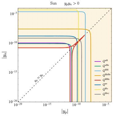
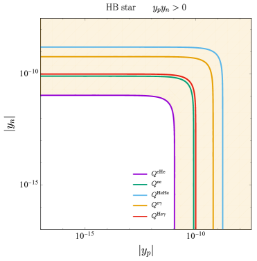
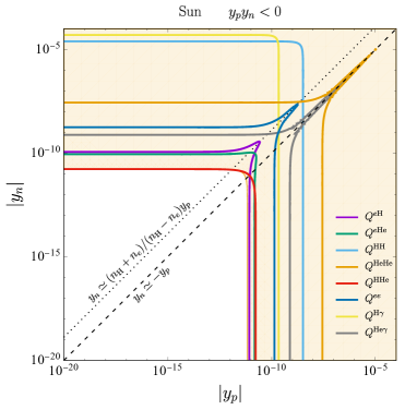
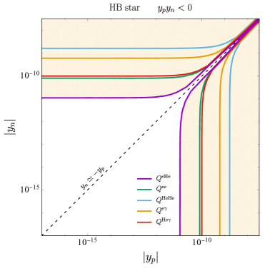
Figure 5: The bounds on the hadrophilic scalar couplings from the stellar cooling: (top) $y_{p}$ and $y_{n}$ are of the same sign and (bottom) they are of opposite signs. (left) the Sun and (right) HB stars. The orange shaded area represent the excluded regions, indicating that the scalar luminosity should be less than $0.03$ ($5$) times the solar luminosity for the Sun (HB stars). $m_{\phi}=10^{-2}$ keV is assumed. As for the dashed and dotted lines, see the text for details.

We begin by discussing the qualitative behaviors in the case of HB stars (the right two panels in Figure 5). Since only helium is effective and its Yukawa coupling appears as the combination $y_{\text{He}}=2(y_{p}+y_{n})$, the constraints on the $(y_{p},\,y_{n})$ plane become symmetric under $y_{p}\leftrightarrow y_{n}$. In addition, a sharp slit is observed in the vicinity of $y_{p}\simeq-y_{n}$, indicating that there is no parameter limit in such a hadrophilic scalar model (the stellaphobic scalar). This behavior of the stellaphobic scalar is not altered even if there exist different or multiple nuclei in stellar medium. This is because, in the absence of hydrogen or isotopes as effective element for the scalar production, the couplings only appear as the combination $y_{p}+y_{n}$, regardless of the inclusion of multi-field medium effects.

In the case of the Sun, as hydrogen is present in addition to helium, the situation is rather different and complicated (the left two panels in Figure 5). One can see several sharp dents and slits in the plots and they are compensated by the effects of multiple fields and processes in the medium. That leads to the constraints on the nucleon couplings even in the region undetectable in the case of HB stars. Let us discuss several qualitative behaviors in order. Firstly, we find that in the small $y_{p}$ region, the bounds are much weaker for the hydrogen processes such as the H-H bremsstrahlung and the H$\gamma$ Compton. The other processes exhibit approximately symmetric bounds with respect to $y_{p}$ and $y_{n}$. Secondly, we consider which processes are dominant. This is a complex problem and involves several independent effects. We find from the figure that the H-He bremsstrahlung is dominant for $|y_{p}|<|y_{n}|$, whereas the $e$-H, $e$-He, and H-He bremsstrahlung contributions become comparable for $|y_{p}|>|y_{n}|$. The reason for this is not immediately apparent. While the $e$-H bremsstrahlung depends on $y_{p}$ in the vacuum, the $y_{n}$ dependence only appears through the multi-field effects in the medium. That leads to somewhat more stringent constraints being placed on $y_{p}$ than $y_{n}$ by the $e$-H bremsstrahlung process. As for the $e$-He bremsstrahlung, both $y_{p}$ and $y_{n}$ should be similarly constrained, but the actual bound is weaker for $y_{n}$. This is because the cancellation occurs in the $y_{n}$-dependent real part of the multi-field factor $c_{\phi}^{e\text{He}}$ near the resonance. Furthermore, as mentioned in Section 2.3, the multi-field effect $c_{\phi}^{X}$ on the nucleus $X$ processes cancels the resonance behavior coming from $z_{\phi}$, if $y_{X}\gtrsim y_{e}$ is satisfied as in the current hadrophilic scenario. This resonance cancellation also holds for $c_{\phi}^{\text{HHe}}$ associated with the H-He bremsstrahlung, since $c_{\phi}^{\text{HHe}}$ is obtained from the combination of $c_{\phi}^{\text{H}}$ and $c_{\phi}^{\text{He}}$. After all, in the case of hadrophilic scalar, the contribution of H-He bremsstrahlung is typically larger than those of other processes, but becomes less significant at the resonance than that of the $e$-H bremsstrahlung. As a result, comparable constraints on the Yukawa couplings can be obtained from three bremsstrahlung processes. These behaviors, which are the consequence of various medium effects, can be seen in Figure 5.

The inclusion of multi-field effects often leads to the cancellation in production amplitudes and generates sharp dents and slits for the parameter constraints. That was observed for the lepton/hadron couplings in the previous section and can also be seen in Figure 5. For the HB stars, there is the slit around $y_{p}+y_{n}\simeq 0$ as mentioned above. On the other hand, the Sun presents a more complex situation, given its composition of multiple nuclei and the inclusion of hydrogen. For $y_{p}y_{n}>0$, the bound from the H-He bremsstrahlung shows a dent approximately at $y_{p}\simeq y_{n}$ where the coefficient of the H-He amplitude vanishes. The other processes or multi-field effects serve to compensate this slit behavior. For $y_{p}y_{n}<0$, we find two distinct types of sharp dents. One corresponds to the helium-like processes observed in $Q^{\text{HeHe}}$ and $Q^{\text{He}\gamma}$. This is similar to the HB star case that a sharp dent appears in the direction where the helium Yukawa coupling vanishes. The other type of dent is observed in the electron-like processes $Q^{e\text{H}}$ and $Q^{ee}$ in the hadrophilic model. These processes occur through the multi-field effect in the Sun, and the contributions from hydrogen and helium nuclei cancel out when $y_{\text{H}}q_{\text{H}}n_{\text{H}}/m_{\text{H}}+y_{\text{He}}q_{\text{He}}n_{\text{He}}/m_{\text{He}}\simeq 0$ (see (B.7)). Under the condition of electrical neutrality, that corresponds to the relation between the nucleon couplings $y_{n}\simeq(n_{\text{H}}+n_{e})/(n_{\text{H}}-n_{e})y_{p}$ (the black dashed line in Figure 5).

4 Summary

In this paper, we have evaluated the scalar production in the medium in the presence of multiple types of fields, particularly including the contributions from heavy fields that are usually ignored. By properly taking the plasmon mixing into account, we have studied how and when multi-field effects are significant. For example, while it has been previously stated that scalar processes are screened in the low-energy regime, our finding indicates that this assertion is valid only for the specific case of a single field/coupling. In the presence of multiple fields and processes, the screening does not occur or is rather weakened. Such an observation means that the inclusion of multiple (heavy) fields/couplings generally induces non-negligible effects in the physics of scalar production in the medium.

As an application, we have analyzed the energy loss due to the scalar emission in stellar interiors. The excessive energy emission affects the evolution of stars and imposes some constraints on the property of scalar particle, such as the mass and couplings. The above medium effects have been included into the evaluation of scalar emission from various processes in the Sun and HB stars. In the stellar medium, where multiple nuclei such as hydrogen and helium exist in addition to the electrons, the multi-field effects appear in various ways, leading to distinct emission rates and resultant parameter constraints. The weakened screening due to multi-field effects, namely the increased production rates at low energy, may not have been a sizable contribution in view of the energy loss, but it could be a crucial element from the perspective of particle number generation.

The presence of heavier nuclei in the system, such as those observed in white dwarfs, might significantly alter the previous analysis. However, it would be necessary to incorporate the treatment of degenerate particles into the current formalism. Moreover, it should be noted that further modifications and corrections may be possible beyond the scope of the present analysis. For example, the contribution from the direct scalar coupling to two photons, higher-order temperature corrections (arising from the velocity expansion of electrons), and corrections due to the mass difference between the proton and neutron could potentially affect the medium effects, especially in the presence of cancellation among the leading-order contributions. It is also theoretically assumed in this paper that the scalar-plasmon two-point function has a certain property, namely that $\Pi_{L\phi}(K)=\Pi_{\phi L}(K)$. This implies that all contributing processes have the same phase, which may change in the presence of CP-violating processes and couplings. Further investigation into these corrections and assumptions is left for future work.

Acknowledgments

The work of Y.Y. was supported by the National Science and Technology Council, the Ministry of Education (Higher Education Sprout Project NTU-112L104022), the National Center for Theoretical Sciences of Taiwan, and the visitor program of Yukawa Institute for Theoretical Physics, Kyoto University. K.Y. is supported by JSPS Grant-in-Aid for Scientific Research KAKENHI Grant Number JP20K03949.

Appendix A Scalar self enery with mixing

We derive the general expression for the self energy of a scalar field $\phi$ in the presence of mixing with other particles. We consider the two-point Green function of $\phi$. When the sum of all one-particle irreducible loop contributions is denoted as $\Pi_{\phi\phi}$, the one-particle irreducible two-point vertex function is obtained by inserting it,

$$-\Gamma_{\phi\phi}^{(0)}{}^{-1}\;=\;\Delta_{\phi}+\Delta_{\phi}\Pi_{\phi\phi}\Delta_{\phi}+\Delta_{\phi}\Pi_{\phi\phi}\Delta_{\phi}\Pi_{\phi\phi}\Delta_{\phi}+\cdots\;=\;(\Delta_{\phi}^{-1}-\Pi_{\phi\phi})^{-1},$$ (A.1)

where $\Delta_{\phi}$ is the tree-level propagator of $\phi$. The superscript $(0)$ means the level at which $\phi$ mixes with other particles. If $\phi$ mixes with the particle $A$ (which, in the text, is identified with the photon in the medium), then the mixing induces additional contributions. When the sum of all one-particle irreducible contributions to the $\phi$-$A$ two-point function is denoted by $\Pi_{\phi A}$, the above vertex function is additionally modified by the contribution with two mixing parts,

$$-\Gamma_{\phi\phi}^{(2)}{}^{-1} \;=\;\Gamma_{\phi\phi}^{(0)}{}^{-1}\Pi_{\phi A}\Delta_{A}\Pi_{A\phi}\Gamma_{\phi\phi}^{(0)}{}^{-1}+\Gamma_{\phi\phi}^{(0)}{}^{-1}\Pi_{\phi A}\Delta_{A}\Pi_{AA}\Delta_{A}\Pi_{A\phi}\Gamma_{\phi\phi}^{(0)}{}^{-1}+\cdots,$$

$$\;=\;\Gamma_{\phi\phi}^{(0)}{}^{-1}\Pi_{\phi A}(\Delta_{A}^{-1}-\Pi_{AA})^{-1}\Pi_{A\phi}\Gamma_{\phi\phi}^{(0)}{}^{-1},$$

$$\;\equiv\;\Gamma_{\phi\phi}^{(0)}{}^{-1}\Pi_{\text{mix}}\Gamma_{\phi\phi}^{(0)}{}^{-1}.$$ (A.2)

$\Delta_{A}$ represents the tree-level propagator of $A$. We have defined $\Pi_{AA}$ as the sum of all one-particle irreducible loop contributions to the two-point function of $A$. While both external lines are $\Delta_{\phi}$ at the tree level, they are replaced by $-\Gamma_{\phi\phi}^{(0)}{}^{-1}$ as described above. Similarly, by inserting $2n$ mixing, we have $-\Gamma_{\phi\phi}^{(2n)}{}^{-1}=-\Gamma_{\phi\phi}^{(0)}{}^{-1}(-\Pi_{\text{mix}}\Gamma_{\phi\phi}^{(0)}{}^{-1})^{n}$. Summing up all the above contributions, we obtain the two-point vertex function $\Gamma_{\phi\phi}$ with the mixing effect,

$$\Gamma_{\phi\phi} \;=\;-\Big{[}\sum_{n=0}-\Gamma_{\phi\phi}^{(0)}{}^{-1}(-\Pi_{\text{mix}}\Gamma_{\phi\phi}^{(0)}{}^{-1})^{n}\Big{]}^{-1}\;=\;\Gamma_{\phi\phi}^{(0)}+\Pi_{\text{mix}}\,.$$ (A.3)

The self energy of $\phi$ is defined by subtracting the tree-level contribution from the two-point vertex function (A.3). We then find the expression of the full self energy $\Pi_{\phi}$ including the mixing effect,

$$\Pi_{\phi}\;=\;\Pi_{\phi\phi}+\Pi_{\text{mix}}\;=\;\Pi_{\phi\phi}-\frac{\Pi_{\phi A}\Pi_{A\phi}}{\Pi_{AA}-\Delta_{A}^{-1}}\,.$$ (A.4)

The evaluation of these one-particle irreducible two-point functions allows for the determination of the damping (thus production/absorption) rate of the field $\phi$ in the medium.

Appendix B Production rates with multiple species of nuclei

This appendix presents the explicit scalar production rates in the case that there exist multiple species of nuclei in the medium. Specifically, we assume three types of fields as in the Sun: electrons ($e$), hydrogen (H), and helium (He). The following processes are appropriate for the production of the scalar field $\phi$ at a temperature typical to the solar interior ($X=$ H, He): (i) $e$-$e$ bremsstrahlung : $e+e\to e+e+\phi$,  (ii) $X$-$X$ bremsstrahlung : $X+X\to X+X+\phi$,  (iii) $e$-$X$ bremsstrahlung : $e+X\to e+X+\phi$,  (iv) $e$ Compton-like : $e+\gamma\to e+\phi$,  (v) $X$ Compton-like : $X+\gamma\to X+\phi$,  (vi) $X$-$X^{\prime}$ bremsstrahlung ($X\neq X^{\prime}$) : $X+X^{\prime}\to X+X^{\prime}+\phi$. The last process is available only when there are two or more nuclei including hydrogen in the medium. When $X,X^{\prime}\neq$ hydrogen, the non-relativistic amplitude of $X$-$X^{\prime}$ bremsstrahlung in the vacuum without mixing is zero as discussed in the text.

Extending the results of Section 2 to the case of two species of heavy particles, the $\phi$ production rate for each process is evaluated including the medium effect factors $z_{\phi}$ and $c_{\phi}$:

$$\Gamma_{\text{prod}}^{ee} \,=\,z_{\phi}c_{\phi}^{e}\frac{q_{e}^{4}y_{e}^{2}n_{e}^{2}T^{1/2}k^{2}J(\omega)}{60\pi^{3/2}m_{e}^{5/2}\omega^{5}}\,,$$ (B.1)

$$\Gamma_{\text{prod}}^{\text{XX}} \,=\,z_{\phi}c_{\phi}^{X}\frac{q_{X}^{4}y_{X}^{2}n_{X}^{2}T^{1/2}k^{2}J(\omega)}{60\pi^{3/2}m_{X}^{5/2}\omega^{5}}\,,$$ (B.2)

$$\Gamma_{\text{prod}}^{eX} \,=\,z_{\phi}c_{\phi}^{eX}\frac{q_{X}^{2}q_{e}^{2}n_{e}n_{X}m_{e}^{1/2}}{3(2\pi)^{3/2}}\Big{(}\frac{y_{e}}{m_{e}}-\frac{y_{X}}{m_{X}}\Big{)}^{2}\frac{k^{2}I(\omega)}{T^{1/2}\omega^{5}}\,,$$ (B.3)

$$\Gamma_{\text{prod}}^{e\gamma} \,=\,z_{\phi}c_{\phi}^{e}\frac{q_{e}^{2}y_{e}^{2}n_{e}f_{\phi}k^{3}}{6\pi m_{e}^{2}\omega^{3}}\,,$$ (B.4)

$$\Gamma_{\text{prod}}^{X\gamma} \,=\,z_{\phi}c_{\phi}^{X}\frac{q_{X}^{2}y_{X}^{2}n_{X}f_{\phi}k^{3}}{6\pi m_{X}^{2}\omega^{3}}\,,$$ (B.5)

$$\Gamma_{\text{prod}}^{XX^{\prime}} \,=\,z_{\phi}c_{\phi}^{XX^{\prime}}\frac{q_{X}^{2}q_{X^{\prime}}^{2}n_{X}n_{X^{\prime}}m_{X}^{1/2}m_{X^{\prime}}^{1/2}}{3(2\pi)^{3/2}(m_{X}+m_{X^{\prime}})^{1/2}}\Big{(}\frac{y_{X}}{m_{X}}-\frac{y_{X^{\prime}}}{m_{X^{\prime}}}\Big{)}^{2}\frac{k^{2}I(\omega)}{T^{1/2}\omega^{5}}\,.$$ (B.6)

$$c_{\phi}^{e} \,=\,\Big{|}\,1+\frac{1}{\omega^{2}}\!\sum_{a=\text{H},\,\text{He}}\!\frac{q_{e}y_{a}-q_{a}y_{e}}{y_{e}m_{a}}\Big{[}q_{a}n_{a}-i\frac{q_{a}}{m_{a}}P_{a}+i\Big{(}\frac{q_{e}}{m_{e}}-\frac{q_{a}}{m_{a}}\Big{)}P_{ea}\Big{]}$$

$$\hskip 56.9055pt-\frac{i}{\omega^{2}}\Big{[}\,\frac{q_{e}}{y_{e}}\Big{(}\frac{y_{\text{H}}}{m_{\text{H}}}-\frac{y_{\text{He}}}{m_{\text{He}}}\Big{)}-\Big{(}\frac{q_{\text{H}}}{m_{\text{H}}}-\frac{q_{\text{He}}}{m_{\text{He}}}\Big{)}\Big{]}\Big{(}\frac{q_{\text{H}}}{m_{\text{H}}}-\frac{q_{\text{He}}}{m_{\text{He}}}\Big{)}P_{\text{HHe}}\,\Big{|}^{2},$$ (B.7)

$$c_{\phi}^{\text{H}} \,=\,\Big{|}\,1+\frac{1}{\omega^{2}}\!\sum_{a=e,\,\text{He}}\!\frac{q_{\text{H}}y_{a}-q_{a}y_{\text{H}}}{y_{\text{H}}m_{a}}\Big{[}q_{a}n_{a}-i\frac{q_{a}}{m_{a}}P_{a}+i\Big{(}\frac{q_{\text{H}}}{m_{\text{H}}}-\frac{q_{a}}{m_{a}}\Big{)}P_{a\text{H}}\Big{]}$$

$$\hskip 56.9055pt-\frac{i}{\omega^{2}}\Big{[}\,\frac{q_{\text{H}}}{y_{\text{H}}}\Big{(}\frac{y_{e}}{m_{e}}-\frac{y_{\text{He}}}{m_{\text{He}}}\Big{)}-\Big{(}\frac{q_{e}}{m_{e}}-\frac{q_{\text{He}}}{m_{\text{He}}}\Big{)}\Big{]}\Big{(}\frac{q_{e}}{m_{e}}-\frac{q_{\text{He}}}{m_{\text{He}}}\Big{)}P_{e\text{He}}\,\Big{|}^{2},$$ (B.8)

$$c_{\phi}^{\text{He}} \,=\,\Big{|}\,1+\frac{1}{\omega^{2}}\!\sum_{a=e,\,\text{H}}\!\frac{q_{\text{He}}y_{a}-q_{a}y_{\text{He}}}{y_{\text{He}}m_{a}}\Big{[}q_{a}n_{a}-i\frac{q_{a}}{m_{a}}P_{a}+i\Big{(}\frac{q_{\text{He}}}{m_{\text{He}}}-\frac{q_{a}}{m_{a}}\Big{)}P_{a\text{He}}\Big{]}$$

$$\hskip 56.9055pt-\frac{i}{\omega^{2}}\Big{[}\,\frac{q_{\text{He}}}{y_{\text{He}}}\Big{(}\frac{y_{e}}{m_{e}}-\frac{y_{\text{H}}}{m_{\text{H}}}\Big{)}-\Big{(}\frac{q_{e}}{m_{e}}-\frac{q_{\text{H}}}{m_{\text{H}}}\Big{)}\Big{]}\Big{(}\frac{q_{e}}{m_{e}}-\frac{q_{\text{H}}}{m_{\text{H}}}\Big{)}P_{e\text{H}}\,\Big{|}^{2},$$ (B.9)

$$c_{\phi}^{e\text{H}} =\,\Big{|}\,1+\frac{1}{\omega^{2}}\frac{q_{e}y_{\text{H}}-q_{\text{H}}y_{e}}{y_{e}m_{\text{H}}-y_{\text{H}}m_{e}}\!\sum_{a=e,\text{H},\text{He}}\!\!\Big{(}q_{a}n_{a}-i\frac{q_{a}}{m_{a}}P_{a}\Big{)}$$

$$\hskip 56.9055pt-\frac{B}{\omega^{2}m_{\text{He}}(y_{e}m_{\text{H}}-y_{\text{H}}m_{e})}\Big{[}\,q_{\text{He}}n_{\text{He}}-i\frac{q_{\text{He}}}{m_{\text{He}}}P_{\text{He}}$$

$$\hskip 113.81102pt-i\Big{(}\frac{q_{e}}{m_{e}}-\frac{q_{\text{He}}}{m_{\text{He}}}\Big{)}P_{e\text{He}}-i\Big{(}\frac{q_{\text{H}}}{m_{\text{H}}}-\frac{q_{\text{He}}}{m_{\text{He}}}\Big{)}P_{\text{HHe}}\,\Big{]}\,\Big{|}^{2},$$ (B.10)

$$c_{\phi}^{e\text{He}} =\,\Big{|}\,1+\frac{1}{\omega^{2}}\frac{q_{e}y_{\text{He}}-q_{\text{He}}y_{e}}{y_{e}m_{\text{He}}-y_{\text{He}}m_{e}}\!\sum_{a=e,\text{H},\text{He}}\!\!\Big{(}q_{a}n_{a}-i\frac{q_{a}}{m_{a}}P_{a}\Big{)}$$

$$\hskip 56.9055pt+\frac{B}{\omega^{2}m_{\text{H}}(y_{e}m_{\text{He}}-y_{\text{He}}m_{e})}\Big{[}\,q_{\text{H}}n_{\text{H}}-i\frac{q_{\text{H}}}{m_{\text{H}}}P_{\text{H}}$$

$$\hskip 113.81102pt-i\Big{(}\frac{q_{e}}{m_{e}}-\frac{q_{\text{H}}}{m_{\text{H}}}\Big{)}P_{e\text{H}}+i\Big{(}\frac{q_{\text{H}}}{m_{\text{H}}}-\frac{q_{\text{He}}}{m_{\text{He}}}\Big{)}P_{\text{HHe}}\,\Big{]}\,\Big{|}^{2},$$ (B.11)

$$c_{\phi}^{\text{HHe}} =\,\Big{|}\,1+\frac{1}{\omega^{2}}\frac{q_{\text{H}}y_{\text{He}}-q_{\text{He}}y_{\text{H}}}{y_{\text{H}}m_{\text{He}}-y_{\text{He}}m_{\text{H}}}\!\sum_{a=e,\text{H},\text{He}}\!\!\Big{(}q_{a}n_{a}-i\frac{q_{a}}{m_{a}}P_{a}\Big{)}$$

$$\hskip 56.9055pt-\frac{B}{\omega^{2}m_{e}(y_{\text{H}}m_{\text{He}}-y_{\text{He}}m_{\text{H}})}\Big{[}\,q_{e}n_{e}-i\frac{q_{e}}{m_{e}}P_{e}$$

$$\hskip 113.81102pt+i\Big{(}\frac{q_{e}}{m_{e}}-\frac{q_{\text{H}}}{m_{\text{H}}}\Big{)}P_{e\text{H}}+i\Big{(}\frac{q_{e}}{m_{e}}-\frac{q_{\text{He}}}{m_{\text{He}}}\Big{)}P_{e\text{He}}\,\Big{]}\,\Big{|}^{2}.$$ (B.12)

$$B\,=\,m_{e}(q_{\text{H}}y_{\text{He}}-q_{\text{He}}y_{\text{H}})+m_{\text{H}}(q_{\text{He}}y_{e}-q_{e}y_{\text{He}})+m_{\text{He}}(q_{e}y_{\text{H}}-q_{\text{H}}y_{e})\,.$$ (B.13)

The functions $P_{i}$, $P_{ij}$, $I(\omega)$, $J(\omega)$ are defined in (2.18)–(2.21). As for the medium effect factors, $z_{\phi}$ is common to all processes, but the multi-field factors $c_{\phi}$ are modified by the existence of two types of nuclei compared to (2.15)–(2.17). In the above expression of $c_{\phi}^{e\text{H}}$, $c_{\phi}^{e\text{He}}$ and $c_{\phi}^{\text{HHe}}$ with the bremsstrahlung, the term $\sum q_{a}n_{a}$ vanishes under the condition of electrical neutrality in the medium. The $\phi$ production rates in the Sun can be obtained by substituting specific values for the electron, hydrogen, and helium in the above general formulae: $q_{e}=-e$, $\,q_{\text{H}}=e$, $\,q_{\text{He}}=2e$, $\,m_{\text{H}}=m_{N}$, $\,m_{\text{He}}=4m_{N}$ ($m_{p}=m_{n}\equiv m_{N}$), and the Yukawa couplings $y_{\text{H}}=y_{p}$, $\,y_{\text{He}}=2y_{p}+2y_{n}$.

References

- [1] G. G. Raffelt, Stars as laboratories for fundamental physics: The astrophysics of neutrinos, axions, and other weakly interacting particles. 5, 1996.
- [2] S. Weinberg, A New Light Boson?, Phys. Rev. Lett. 40 (1978) 223–226.
- [3] F. Wilczek, Problem of Strong and Invariance in the Presence of Instantons, Phys. Rev. Lett. 40 (1978) 279–282.
- [4] R. D. Peccei and H. R. Quinn, CP Conservation in the Presence of Instantons, Phys. Rev. Lett. 38 (1977) 1440–1443.
- [5] B. Holdom, Two U(1)’s and Epsilon Charge Shifts, Phys. Lett. B 166 (1986) 196–198.
- [6] L. B. Okun, Limits of electrodynamics: paraphotons?, Sov. Phys. JETP 56 (1982) 502.
- [7] J. McDonald, Gauge singlet scalars as cold dark matter, Phys. Rev. D 50 (1994) 3637–3649, arXiv:hep-ph/0702143.
- [8] M. Pospelov, A. Ritz, and M. B. Voloshin, Secluded WIMP Dark Matter, Phys. Lett. B 662 (2008) 53–61, arXiv:0711.4866 [hep-ph].
- [9] A. Fradette, M. Pospelov, J. Pradler, and A. Ritz, Cosmological beam dump: constraints on dark scalars mixed with the Higgs boson, Phys. Rev. D 99 (2019) 075004, arXiv:1812.07585 [hep-ph].
- [10] H. An, M. Pospelov, and J. Pradler, New stellar constraints on dark photons, Phys. Lett. B 725 (2013) 190–195, arXiv:1302.3884.
- [11] J. Redondo and G. Raffelt, Solar constraints on hidden photons re-visited, JCAP 08 (2013) 034, arXiv:1305.2920.
- [12] J. H. Chang, R. Essig, and S. D. McDermott, Revisiting Supernova 1987A Constraints on Dark Photons, JHEP 01 (2017) 107, arXiv:1611.03864.
- [13] E. Hardy and R. Lasenby, Stellar cooling bounds on new light particles: plasma mixing effects, JHEP 02 (2017) 033, arXiv:1611.05852.
- [14] P. S. B. Dev, R. N. Mohapatra, and Y. Zhang, Revisiting supernova constraints on a light CP-even scalar, JCAP 08 (2020) 003, arXiv:2005.00490.
- [15] G. B. Gelmini, V. Takhistov, and E. Vitagliano, Scalar direct detection: In-medium effects, Phys. Lett. B 809 (2020) 135779, arXiv:2006.13909.
- [16] N. V. Mikheev, G. Raffelt, and L. A. Vassilevskaya, Axion emission by magnetic field induced conversion of longitudinal plasmons, Phys. Rev. D 58 (1998) 055008, arXiv:hep-ph/9803486.
- [17] A. K. Ganguly, P. Jain, and S. Mandal, Photon and axion oscillation in a magnetized medium: A general treatment, Phys. Rev. D 79 (2009) 115014, arXiv:0810.4380.
- [18] A. Caputo, A. J. Millar, and E. Vitagliano, Revisiting longitudinal plasmon-axion conversion in external magnetic fields, Phys. Rev. D 101 (2020) 123004, arXiv:2005.00078.
- [19] M. L. Bellac, Thermal Field Theory. Cambridge Monographs on Mathematical Physics. Cambridge University Press, 3, 2011.
- [20] M. Laine and A. Vuorinen, Basics of Thermal Field Theory, vol. 925. Springer, 2016. arXiv:1701.01554.
- [21] H. A. Weldon, Simple Rules for Discontinuities in Finite Temperature Field Theory, Phys. Rev. D 28 (1983) 2007.
- [22] S.-P. Li and X.-J. Xu, Production rates of dark photons and Z’ in the Sun and stellar cooling bounds, JCAP 09 (2023) 009, arXiv:2304.12907.
- [23] M. A. Shifman, A. I. Vainshtein, M. B. Voloshin, and V. I. Zakharov, Low-Energy Theorems for Higgs Boson Couplings to Photons, Sov. J. Nucl. Phys. 30 (1979) 711–716.
- [24] S. Bottaro, A. Caputo, G. Raffelt, and E. Vitagliano, Stellar limits on scalars from electron-nucleus bremsstrahlung, JCAP 07 (2023) 071, arXiv:2303.00778.
- [25] Y. Yamamoto and K. Yoshioka, Stellar cooling limits on light scalar boson revisited, Phys. Lett. B 843 (2023) 138027, arXiv:2303.03123.
- [26] N. Vinyoles, A. M. Serenelli, F. L. Villante, S. Basu, J. Bergström, M. C. Gonzalez-Garcia, M. Maltoni, C. Peña Garay, and N. Song, A new Generation of Standard Solar Models, Astrophys. J. 835 (2017) 202, arXiv:1611.09867.
- [27] N. Vinyoles, A. Serenelli, F. L. Villante, S. Basu, J. Redondo, and J. Isern, New axion and hidden photon constraints from a solar data global fit, JCAP 10 (2015) 015, arXiv:1501.01639.
- [28] G. Grilli di Cortona, E. Hardy, J. Pardo Vega, and G. Villadoro, The QCD axion, precisely, JHEP 01 (2016) 034, arXiv:1511.02867.