The case for adopting the sequential Jacobi’s diagonalization algorithm in neutrino oscillation physics

Abstract

Neutrino flavor oscillations and conversion in the presence of an interacting background may offer the missing evidence for charge-parity violation in the leptonic sector of the Standard Model, as well as yet undiscovered new interactions. The usual approach for simulating these effects is by numerically integrating the Schrödinger equation over the neutrino trajectory, arriving at the conversion and survival probabilities for each flavor. From these, the neutrino mixing matrix and its parameters are recovered. This work makes the case for a different numerical approach, which starts by recognizing how Jacobi’s diagonalization algorithm is the most suitable for neutrino oscillations in general. By switching from physical space to a parameter space of choice, Jacobi’s algorithm results in both eigenvalues and eigenvectors simultaneously, with only local round-off errors. This approach is trivially parallelizable, making it a suitable choice for concurrent computation. Moreover, the freedom to build a parameter space allows for quasi-model-independent solutions, which in turn eliminates the necessity of repeating the simulation for every change in the model’s parameters. Benchmarks and efficiency analyses are discussed, as well as a concrete neutrino oscillation example.

1 Introduction

Neutrino oscillations, like many other quantum mechanical systems, are described by the evolution of matrices over time. Different from other systems, however, the interpretation of oscillation parameters within the Standard Model (SM) of particle physics is given by the Pontecorvo–Maki–Nakagawa–Sakata (PMNS) parametrization. Among other characteristics, the PMNS attributes physical meaning to the ordering of the neutrino mass eigenstates, which in turn allow us to experimentally probe such order. Numerical methods for matrix diagonalization do not carry information about the eigenvalues’ ordering. Since ordering is related to an arbitrary choice of basis, the algorithm is agnostic about that choice and will, in fact, produce results in a random order. This is the same effect seen when trying to predict to which root of a polynomial the application of the Newton-Raphson method will converge, depending on the initial conditions, also known as Newton’s Fractal[1]. . This lack of predictable ordering precludes widespread use of numerical diagonalization algorithms in neutrino physics. Instead, the Schrödinger equation describing the system is solved numerically and the PMNS parameters, i.e., the mixing angles, squared-mass differences and Charge-Parity (CP) violation phase, are recovered from the solution. This procedure becomes computationally intensive the more feature the underlying model has, such as inhomogeneous backgrounds and flavor-changing Beyond Standard Model (BSM) interactions, which are quite common in the neutrino research field.

In what follows, an existing numerical approach for the diagonalization of Hermitian matrices is reviewed, namely the Jacobi method, with the addition of an extra steps to ensure the preservation of any preexisting parametrization. This is accomplished by sequentially comparing the eigenvalues over a defined and smooth path in small discrete steps, transporting the ordering of the eigensystem across the parameter space. This algorithm offers advantages to neutrino physicists, mainly when simulating an active interacting medium and how it affects the neutrino’s oscillation pattern[2, 3]. See Refs. [4, 5] and [6] for excellent reviews. Although analytical solutions do exist for the most common scenarios[7, 8], these are SM dependent and cannot be easily expanded for more general models, such as on the study of non-standard neutrino interactions and sterile neutrinos. Since future experiments such as the Deep Underground Neutrino Experiment (DUNE)[9] will be able to explore BSM physics, new algorithms with better computational complexity are required. In what follows, the case for using the Jacobi algorithm is made base on several computational aspects, including efficiency, precision and concurrency. In the remainder of this text, the words parametrization and ordering are used interchangeably since, in the context of neutrino oscillations, one implies the other.‘gt

This paper is organized in such manner as to allow the reader to first understand the method being presented, and later deal with its validation and application. Sec. 2 defines the problem; Sec. 3 reviews the original Jacobi algorithm for a Hermitian matrix; Sec. 4 outlines the sequential method, which ensures parametrization over a continuous path; and Sec. 5 presents the general conclusions. After this, a series of three appendices showcase discussions and details that might not be of interest for the general reader: A contains an analysis of convergence, precision and stability of the algorithm; B performs a benchmark test by solving a random case and comparing it with its analytical solution; and finally C discusses the application in neutrino physics, presenting an example which can also be compared with analytical solutions.

2 Parametrized Hermitian Matrices

Let $A$ be a Hermitian matrix of order $n$, with $n(n-1)/2$ independent elements $A_{jk}\in\mathbb{C}$. Consider the case where each element is given by a continuous function over a $p$-dimensional parameter space, i.e., $A_{jk}\equiv A_{jk}(\vec{q})$, with $\{\vec{q}=(q_{1},\ldots,q_{p})\,|\,\vec{q_{i}}\in\mathbb{R}\}$. The eigensystem of $A$ is the set of real eigenvalues $\lambda_{k}$ and the corresponding eigenvectors $V_{k}$. The latter spans into an orthogonal linear space, even in the case of degeneracy between eigenvalues. The spectral theorem ensures that all Hermitian matrices are normal matrices and it is always possible to write $A=U\ D\ U^{\dagger}$, where $D=\mbox{diag}\left(\lambda_{1},\lambda_{2},\ldots,\lambda_{n}\right)$ and

$$U=\left[\begin{array}[]{cccc}\left(\!\!\begin{array}[]{c}\vdots\\ V_{1}\\ \vdots\\ \end{array}\!\!\right)\left(\!\!\begin{array}[]{c}\vdots\\ V_{2}\\ \vdots\\ \end{array}\!\!\right)\begin{array}[]{c}\\ \cdots\\ \\ \end{array}\left(\!\!\begin{array}[]{c}\vdots\\ V_{n}\\ \vdots\\ \end{array}\!\!\right)\end{array}\right]$$ (14)

where $U$ is a unitary matrix and, not only each column $V_{k}$ is the corresponding eigenvector to $\lambda_{k}$, but they are also in the same order as they appear in $D$. From this point foreword the eigensystem of $A$ is represented by the pair of matrices $\{D,U\}$, so that the ordering information is well defined. We are interested in describing the eigensystem as a function of the original parametrization. In other words, given that $A(\vec{q})$ is parametrized, so must be $D(\vec{q})$ and $U(\vec{q})$. The ordering of the $\lambda_{k}$ in $D$ might be a free choice, but is assumed to have physical meaning and it has to be preserved. Before discussing the ordering issue, however, let us review the diagonalization method that is more suitable for this task, the Jacobi-Given method.

3 Jacobi’s Algorithm

The original algorithm proposed by Carl G. J. Jacobi in 1845[10] established a numerical procedure to calculate eigenvalues of a real, symmetric matrix. Since then, several variations were developed in the literature, including an extension to a general complex matrix[11, 12]. The focus of this work is the diagonalization of Hermitian matrices, which is reviewed in this section, for completion sake (with notation and steps mainly based on Ref. [13]).

Consider $A$ a Hermitian matrix, and $d^{2}$ a measure the magnitude of its off-diagonal elements, defined as

$$d^{2}=\frac{2}{n(n-1)}\sum_{i>j}^{n}A_{ij}\,A_{ji}\,,$$ (15)

where $A_{ji}=A_{ij}^{\star}$ by definition. There exists an infinite sequence $\left\{A_{0},\,A_{1},\,\cdots\,A_{k},\,A_{k+1},\cdots\right\}$, with general term

$$A_{k+1} = S_{k}^{\dagger}\,A_{k}\,S_{k}\,\,,\hskip 14.22636pt\mbox{or}$$

$$= S_{k}^{\dagger}S_{k-1}^{\dagger}\cdots S_{0}^{\dagger}\,\,A_{0}\,\,S_{0}\cdots S_{k-1}S_{k}\,,$$

so that the sequence of corresponding measurements $\left\{d^{2}_{0},\,d^{2}_{1},\,\cdots\,d^{2}_{k}\,,\cdots\right\}$ converges to zero when $k\rightarrow\infty$. In other words, $A_{k}$ converges to a diagonal matrix. From the definitions on Sec. 2, $A$ can be factored as a diagonal matrix $D$ and an unitary transformation $U$, as $A=U\ D\ U^{\dagger}$. This relation can be inverted in order to express $D$ as a function of $A$ and $U$,

$$D=U^{\dagger}\ A\ U$$ (17)

which is recognizable as the limit of Eq. 3, as $A_{k}\rightarrow D$ when $A=A_{0}$. From the perspective of a numerical approximation, we may stop the sequence $\left\{A_{k}\right\}$ when the condition $d_{k}^{2}\leq\varepsilon^{2}$ is met, for an arbitrary precision $\varepsilon$. In this case, Eq. 3 leads to

$$D \approx A_{k}=S^{\dagger}\,A_{0}\,S\ ,\mbox{for large enough }k,$$ (18)

and

$$U \approx S\ \mbox{, with }\ S\equiv S_{0}\,S_{1}\,\ldots S_{k}\ ,$$ (19)

with a global truncation error $E\leq\varepsilon$.

Several strategies are available to construct a sequence of rotations that satisfies these definitions. The total computational complexity (and time) depends on the number of steps in the sequence and the time devoted to each one. In particular, the $S_{k}$ can be organized in groups called sweeps where all the off-diagonal elements are systematically rotated way, one by one, in what is known as Cyclic Jacobi Method (CJM)[12, 14, 15]. This strategy requires no decision making regarding the elements themselves, thus employing the least amount of time per step. Another option is to eliminate the largest remaining off-diagonal element with each rotation, which is Jacobi’s original strategy [10]. This strategy leads to a quadratic convergence, at the cost of a search for the largest element. This is the method implemented here, but I encourage the reader to compare both strategies before tackling problems where large matrices are involved. For a modern review and variations on the implementation presented here, refer to Ref. [13] and references therein. In what follows, the classical Jacobi’s strategy is used.

A Jacobi rotation $S_{k}$ represents a single step in the process of diagonalizing the target matrix $A$, and it is applied on the largest off-diagonal element, $A_{rc}$, with $r\neq c$ being the row $r$ and column $c$. Each $S_{k}$ can be decomposed into two consecutive rotations, $S_{k}=K^{[rc]}\,G^{[rc]}$. Each of these independent rotations $K$ and $G$ is responsible for rotating away one of the two degrees of freedom of this element, since $A_{rc}$ is a complex number. In other words, the first rotation $A^{\prime}=K^{\dagger[rc]}AK^{[rc]}$ makes the resulting element $A^{\prime}_{rc}$ real, while the second one $A^{\prime\prime}=G^{\dagger[rc]}A^{\prime}G^{[rc]}$ is responsible for vanishing with $A^{\prime\prime}_{rc}$. Under these requirements, $K^{[rc]}$ may be written as

$$\!\!\!\!\!\!K^{[rc]}=\frac{1}{\sqrt{2}}\left[\begin{array}[]{ccccc}1&&&&\\ &e^{i\theta_{1}}&\cdots&e^{-i\theta_{1}}&\\ &\vdots&1&\vdots&\\ &-e^{i\theta_{1}}&\cdots&e^{-i\theta_{1}}&\\ &&&&1\end{array}\right],$$ (20)

with the main elements given by $K^{[rc]}_{rr}=e^{+i\theta_{1}}/\sqrt{2}=K^{\star[rc]}_{cc}$, $K^{[rc]}_{rc}=e^{i\theta_{1}}/\sqrt{2}=-K^{\star[rc]}_{cr}$, and $K^{[rc]}_{jj}=1$ for the diagonal elements, except at $rr$ and $cc$. All other elements are null. By imposing that $Im\{A^{\prime}_{rc}\}=0$, the rotation angle $\theta_{1}$ becomes

$$\tan 2\theta_{1}=\frac{Im\left\{A_{rc}\right\}}{Re\left\{A_{rc}\right\}}\ .$$ (21)

In the case where the target matrix $A$ is already real, $\theta_{1}=0$ and $K^{[rc]}$ becomes the identity $1$. The second transformation $G^{[rc]}$ must be a real rotation,

$$G^{[rc]}=\left[\begin{array}[]{ccccc}1&&&&\\ &\cos\theta_{2}&\cdots&\sin\theta_{2}&\\ &\vdots&1&\vdots&\\ &-\sin\theta_{2}&\cdots&\cos\theta_{2}&\\ &&&&1\end{array}\right],$$ (27)

with notation analogous to the one used on Eq. 20, $G^{[rc]}_{rr}=\cos\theta_{2}=K^{[rc]}_{cc}$, $K^{[rc]}_{rc}=\sin\theta_{2}=-K^{[rc]}_{cr}$, with $K^{[rc]}_{jj}=1$ for the diagonal elements, except at $rr$ and $cc$, and all others being null. The rotation angle $\theta_{2}$ is given by

$$\tan 2\theta_{2}=\frac{2\,A^{\prime}_{rc}}{A^{\prime}_{cc}-A^{\prime}_{rr}}\ .$$ (28)

The texture and parametrizations chosen for these rotations are known as Givens rotations, after W. Givens[13]. They facilitate the derivation and application of this method, but extra care should be taken when calculating the angles $\theta_{1}$ and $\theta_{2}$ since Eqs. 21 and 28 are prone to overflow, when numerically evaluating $\tan^{-1}$.

Details of how efficient and accurate the Jacobi’s algorithm is, are presented in A. Next, a heuristic approach is presented with the goal to preserve the ordering of a given eigensystem.

4 Sequential Diagonalization

As previously discussed in Sec.2, once the parametrization of a Hermitian matrix is defined, the objective is obtain the dependency of its eigensystem without randomizing the basis ordering. The approach proposed here is to perform a sequential diagonalization, summarized as follows:

• Starting from a point in parameter space where the eigensystem is known (including ordering), a small step is given to a new position;

• The eigensystem is obtained in this new position and a comparison is drawn between the original set of eigenvalues and the new ones;

• Assuming that the step is short enough, it is always possible to arrive at an one-to-one match between the two sets, which allows the post-step eigensystem to be reordered following their pre-step counterparts;

• This is now regarded as the reference value and the process is repeated over a predefined path, transporting the known parametrization along it.

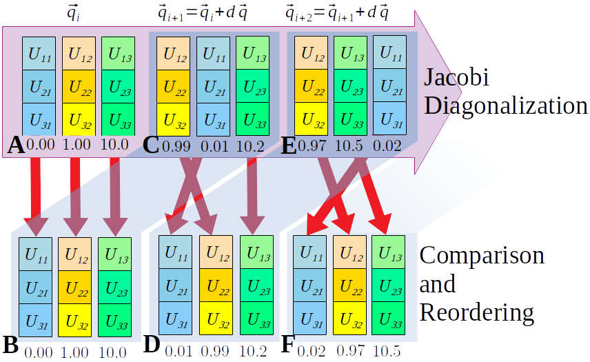
Figure 1: Sequential Jacobi Diagonalization. Schematics showing the evolution a Hermitian matrix’s eigensystem, at a few steps along the parametrization path. The resulting diagonalizing transformation $U$ is shown, where each column represents an eigenvector, with its corresponding eigenvalue marked below it. A is the starting point, representing the ordering to be preserved. It is stored as the first reference, shown in B; After a small step $d\vec{q}$, a new eigensystem is obtained with the Jacobi method, shown as C. This is compared with the previous reference, using Eq. 33, in order to know the correct way to reorder C to match B; C is stored as a new reference and the cycle repeats for the next step E. In summary, while A, C and E result from the diagonalization, with random ordering, B, D and F are the values actually stored.

From the definitions in Sec. 2, the relation $A=U\ D\ U^{\dagger}$ defines the pair $\{D,U\}$ representing $A$’s eigensystem. The diagonal form of $A$ is $D(\vec{q})\equiv\mbox{diag}(\lambda_{1}\cdots\lambda_{n})$, with $\lambda_{k}(\vec{q})$, while the collection of eigenvectors $V_{k}(\vec{q})$ is organized as the columns of $U(\vec{q})$ as defined in Eq. 14. In order to obtain $\{D,U\}$ at a given point $\vec{q}_{\star}\neq\vec{q}_{0}$, a path between the two points is drawn, $\vec{q}(t)$, as a function of a single parameter $t$. This new parametrization has now physical meaning and it is unrelated to how $A$ is parametrized over $\vec{q}$. This relation is introduced to reduce the number of degree of freedom (d.o.f.) from $p$ parameters to a single one, $t$. The path connecting $\vec{q}(t=t_{i})=\vec{q}_{0}$ and $\vec{q}(t=t_{f})=\vec{q}_{\star}$ can be chosen with any criteria in mind, including simplifying the calculations. The path is then divided into smaller steps $\delta t\ll 1$ in total of $N=1/\delta t$ steps. Without any loss of generality, we might consider a straight line,

$$\vec{q}(t)=\vec{q_{0}}+\left(\frac{t-t_{i}}{t_{f}-t_{i}}\right)(\vec{q_{\star}}-\vec{q_{0}})$$ (29)

as long as $\vec{q}(t)$ never leaves the domain of $A(\vec{q})$. When this is not feasible, Eq. 29 can be generalized by a series of line segments or a curve of any kind. Nevertheless, the reader should keep in mind that the resulting $\{D,U\}$ are independent of the taken path, so the curve $\vec{q}(t)$ should be as simple as possible. From this point forward consider that Eq.29 is enough to define $\vec{q}(t)$. In this case, a short step $\delta t$ leads to a step $\delta\vec{q}$, with

$$\delta\vec{q}=\left(\vec{q_{\star}}-\vec{q_{0}}\right)\delta t$$ (30)

with

$$\vec{q}_{i+1}=\vec{q}_{i}+\delta\vec{q}$$ (31)

being the discrete representation of the chosen path. At any given step $i$, the next step will lead to $A_{i+1}=A(\vec{q}_{i+1})=A(\vec{q}_{i}+\delta\vec{q})$. When diagonalized, the resulting eigenvalue set $\{\lambda^{(i+1)}_{k}\}$ should have the form

$$\lambda^{(i+1)}_{k}=\lambda^{(i)}_{k}+\delta\lambda_{k}\ .$$ (32)

This relation can be used as a tool to correct for the ordering of $\{\lambda^{(i+1)}_{k}\}$, by defining the quantity

$$\Delta=\sum_{k=0}^{n}\left|\lambda^{(i+1)}_{k}-\lambda^{(i)}_{k}\right|$$ (33)

it is possible to search for the correct ordering of $\lambda^{(i+1)}$ among all possible permutations. Given that $\delta t$ is small enough, the relation $\Delta<(n\ \mbox{max}\{\lambda_{k}\})$ can only be true if the ordering of $\{\lambda^{(i+1)}_{k}\}$ matches the previous one for $\lambda^{(i)}_{k}$. This is performed by simple inspection, placing all permutations of $\{\lambda^{(i+1)}_{k}\}$ in the definition of $\Delta$ and choosing the smallest one. Once the correct permutation is known, both $\{\lambda^{(i+1)}_{k}\}$ and $\{V^{(i+1)}_{k}\}$ can be reordered and stored in $\{D_{i+1},U_{i+1}\}$. Step by step, the procedure is repeated until the end point is reached, leading to the desired $\{D_{\star},U_{\star}\}$. Fig. 1 illustrates two consecutive steps of the algorithm.

The sequential diagonalization just described can be used alongside any diagonalization method, including analytical ones. It is worth noting however that Jacobi’s method is the best fit since it offers the possibility of evaluating both $D$ and $U$ at the same time with precision $\varepsilon$ predefined by the stopping condition. In fact, since only the ordering information is passed from one point to the next, there are no cumulative numerical errors involved. In other words, the only errors affection $(D_{\star},U_{\star})$ are those coming from the last diagonalization, at the point $\vec{q_{\star}}$ (more on A).

This method is not without its limitations. The sequential diagonalization relies on the premise that there is a reference order. As a consequence, the eigenvalues have to be non-degenerated to begin with. Not only that, but they have to be different enough so Eq.33 is applicable. It could be the case, however, that some particular parametrization causes two or more eigenvalues to cross each other, becoming degenerate at that point. This kind of ambiguity can be solved by adopting a higher order discriminant, such as comparing $\lambda^{i+1}_{k}$ with $\lambda^{i-1}_{k}$, which is equivalent to comparing the derivatives of $d\lambda_{k}/dt$. Another shortcoming is the ordering inspection, which takes $n!-1$ comparisons in order to account for all possible permutations. For increasing dimensionalities this will become the most expensive operation since the diagonalization complexity is $n^{2}$. One way to minimize this is to use the fact that not all steps need reordering. In fact, although the eigenvalues appear to switch places randomly, practice shows that the largest likelihood is for either none or just a few permutations to occur. So the application of Eq.33 should remember the permutation found at the last step, and test it first. In general, the possible permutations of the original order should be checked by first considering the ones with the least number of changes, progressively testing the ones with the most. This strategy limits the cost of the comparison significantly. Moreover, it is worth noting that a significant part of the algorithm can be performed in parallel. Only the comparison and reordering is sequential, while the diagonalizations at every point $\vec{q}$ are independent, and can be performed in multi-thread. The sequential reordering can be applied to a previously diagonalized set of $\{D,U\}$, gaining computational time.

5 Conclusions

The Sequential Jacobi Diagonalization proposed in this work combines a heuristic procedure with a well established numerical method in order to satisfy the computation requirements for neutrino physics applications. In this field, computational resources become a bottleneck whenever BSM hypotheses are being tested. In more general terms, given the description of a Hermitian system, modeled over a particular set of parameters, this method allows for the study of how the eigenvalues and eigenvectors are related to these parameters.

Appendix A Precision and Efficiency

In order to evaluate stability, convergence and precision, I applied the Jacobi diagonalization to a sample of $10^{6}$ random Hermitian matrices, with the real and imaginary parts of each element constrained to $[-1,+1]$. This sample is representative since any matrix can be normalized by its largest element in order to fit in this range. After reaching the stop condition $d^{2}\leq\varepsilon^{2}$, as defined on Eq. 15, the resulting diagonal form is rotated back with the obtained $U=S^{\dagger}$, and compared component-wise with the original matrix. The largest difference is found to be always smaller than the target precision $\varepsilon$, meaning that $-\log_{10}\varepsilon$ is a good indicator of the number of significant figures achieved in the solutions. For each sample, $\varepsilon$ is varied from $10^{-2}$ to $10^{-16}$, where the average number of rotations $S_{k}$ is recorded. This virtual experiment is repeated from $n=3$ to $n=10$ matrices and the results are shown in Fig. 2.

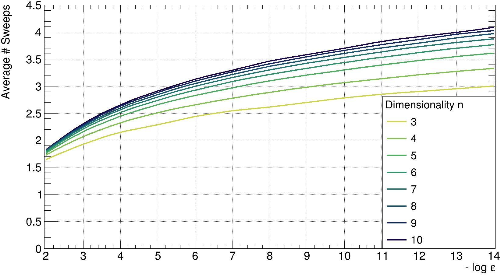
Figure 2: Average number of sweeps before converging to a diagonal, with given precision $\varepsilon$ (shown as $-\log\varepsilon$). One sweep is defined as the application of one full complex rotation for each off-diagonal element, $n(n-1)/2$. Each line represent a dimensionality from $n=3$ to $10$. This average is obtained from a random sample of $10^{6}$ Hermitian matrices with real and imaginary parts limited to the interval $[-1,+1]$. It is possible to obtain diagonalizations with the largest off-diagonal element bounded as $<10^{-14}$ by employing an average of 3 to 4 sweeps, for matrices up to $10\times 10$.

Since the method targets the largest elements, not all in sequence (contrary to its cyclic variant), the average “sweep” is defined as the ratio between the number of complex rotations (two real rotations from Eq.20 and 27) and the number of off-diagonal elements $n(n-1)/2$. This ratio is strictly larger than $1$, regardless of the dimensionality, since a general matrix requires at least one complex rotation for each off-diagonal element. The actual number of rotations goes with $\mathcal{O}(n^{2})$. By establishing the $d^{2}\leq\varepsilon^{2}$ limit from Eq. 15 as stopping criterion, there is a possibility that some elements might underflow if the required $\varepsilon$ is too close to machine precision. Indeed, this is observed when requiring $\varepsilon\leq 10^{-15}$, using 64-bit floating-point variables (which can represent a maximum of $15$ significant figures). Stability and convergence are observed with $\varepsilon\geq 10^{-14}$, which is the largest precision shown in Fig. 2. In this limit, numerical diagonalization is achieved with an average of between $3$ and $4$ sweeps. This average held even for matrices as large as $10\times 10$. Most physical applications would realistic require far less precision than the $10^{-14}$ tested, which translates to a less demanding process. Tab.1 shows the average number of sweeps, the standard deviation, and how many sweeps are needed to diagonalize $99\%$ of each sample. Even in the most demanding case, with $n=30$, a five significant figures precision can be obtained with a maximum of $3.2$ sweeps. Also, the standard deviation around this average gets narrower as $n$ increases. Both Fig.2 and Tab.1 show evidence of a possible limit, or at least a log-like growth, in the number of sweeps as a function of $n$. This cannot be verified by employing only numerical analysis, so no further statements will be made on this observation. It can be said however, that the expected number of real rotations is $3n^{2}$, as a thumb-rule. As a final remark, quadratic convergence (precision = $\mbox{sweeps}^{2}$) was observed for all tested dimensionalities, as suggested by the literature[12].

n	Avg. Sweeps	Std. dev.	$99\%$ less than
3	2.30	0.19	2.7
4	2.51	0.19	3.0
5	2.66	0.13	3.1
6	2.74	0.10	3.1
7	2.81	0.10	3.1
8	2.85	0.09	3.2
9	2.88	0.08	3.2
10	2.92	0.08	3.2
20	3.07	0.05	3.2
30	3.15	0.04	3.3

Table 1: Average number of sweeps required for convergence a diagonal, with precision $\varepsilon=10^{-5}$, from the a $10^{6}$ random matrices sample. The first column (Avg. Sweeps) corresponds to a cut from Fig.2 at $-\log\varepsilon=5$. The second one (Std. dev.) shows the standard deviation from each sample. The rightmost column shows how many sweeps were needed for $99\%$ of each sample to reach the stopping condition. The two bottom rows show extra information not present in Fig.2, for $n=20$ and $n=30$. Even with such large matrices, less than $1\%$ of the matrices reacquired more than $3.3$ sweeps.

Appendix B Numerical vs. Analytical

In this section, a random example with an analytic solution is analyzed. The goal is to validate the numerical methods proposed in this work. A particular $n=3$ case with a known analytic solution is used to exemplify the validity of the method. Starting with two Hermitian matrices, $A$ and $B$, given by

$$A=\left[\begin{array}[]{ccc}\!\!3&\!\!i&\!\!0\\ -i&-2&\!\!i\\ 0&-i&\!\!1\end{array}\right],$$ (B.4)

and

$$B=\left[\begin{array}[]{ccc}1&0&0\\ 0&2&0\\ 0&0&3\end{array}\right],$$ (B.8)

a linear parametrization is defined as

$$H(x)=A\ x+B\ .$$ (B.9)

These were chosen among several tests for no particular reason other than to provide a good example. The eigenvalues of $B$ are not only explicit, since $B$ is diagonal by definition, but also their ordering is well determined. The eigenvalues of $A$ are obtained by solving its order-3 characteristic polynomial, leading to

$$\lambda_{1}^{A} = \frac{1}{3}\left[2-\mbox{Re}\left\{\sigma\ (1-i\sqrt{3})\right\}\right]\ ,$$ (B.10)

$$\lambda_{2}^{A} = \frac{1}{3}\left[2+\mbox{Re}\{\sigma\}\right]\ ,$$ (B.11)

and

$$\lambda_{3}^{A} = \frac{1}{3}\left[2-\mbox{Re}\left\{\sigma\ (1+i\sqrt{3})\right\}\right]\ ,$$ (B.12)

where $\sigma=(-64+3i\sqrt{1281})^{1/3}$ (the first complex root). Their numbering is reflecting their relative positioning on the number line, $\lambda_{1}^{A}\geq\lambda_{2}^{A}\geq\lambda_{3}^{A}$, not parametrization ordering. For the sake of this analysis, all numerical values are quoted with $10^{-5}$ precision even when using analytical formulas. The eigenvalues of $A$ are $\lambda_{1}^{A}=-2.47090$, $\lambda_{2}^{A}=1.26071$, and $\lambda_{3}^{A}=3.21018$, as defined by Eqs. B.10, B.11, and B.12.

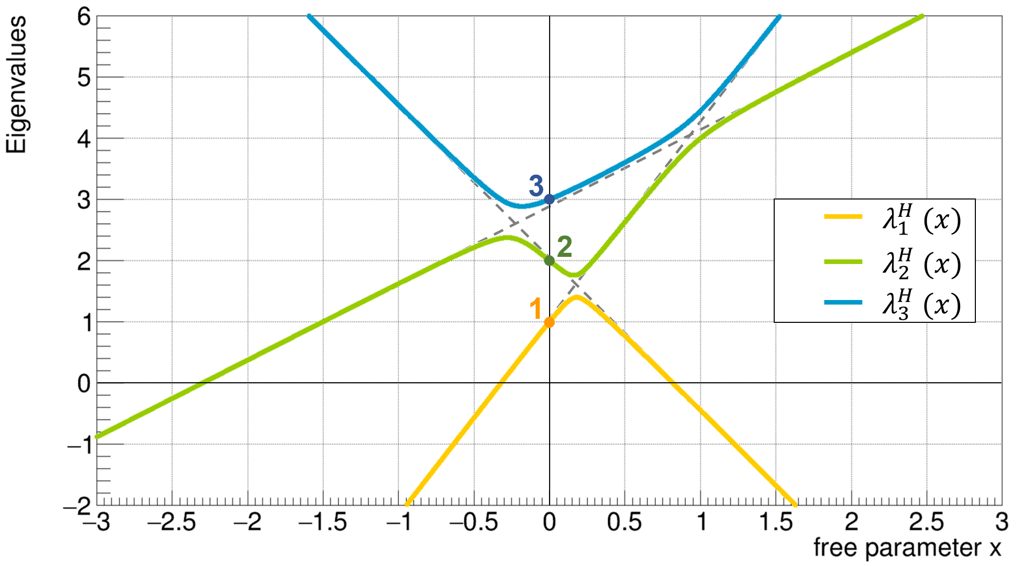
(a) eigenvalues of $H(x)$.

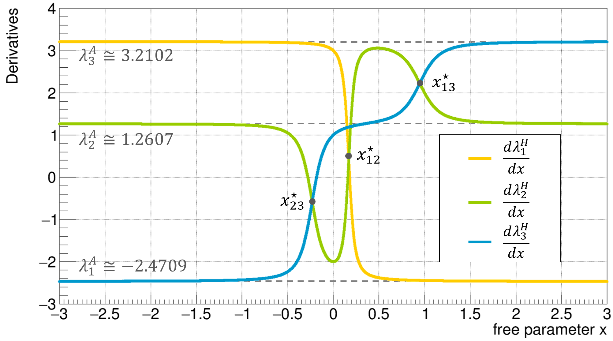
(b) Derivative of the eigenvalues of $H(x)$.

Figure 3: (a) Eigenvalues of $H(x)$, as defined by Eqs. B.4, B.8 and B.9. The continuous lines shows $\lambda_{1}^{H}$ (yellow), $\lambda_{2}^{H}$ (green) and $\lambda_{3}^{H}$ (blue), as a function of the free parameter $x$. The dashed lines indicate the asymptotes (Eq.B.13) and their intersections (Tab.B.1). (b) Derivative of the Eigenvalues of $H(x)$ with respect to $x$, as defined by Eqs. B.4, B.8 and B.9. The continuous lines shows $d\lambda_{1}^{H}/dx$ (yellow), $d\lambda_{2}^{H}/dx$ (green) and $d\lambda_{3}^{H}/dx$ (blue), as a function of the free parameter $x$. The dashed lines indicate the asymptotes (Eq.B.13), which correspond to the eigenvalues of $A$ listed in Eqs.B.10, B.11, and B.12. Their intersections correspond to those of the asymptotes defined by Eq.B.13 and their numerical values displayed on Tab. B.1.

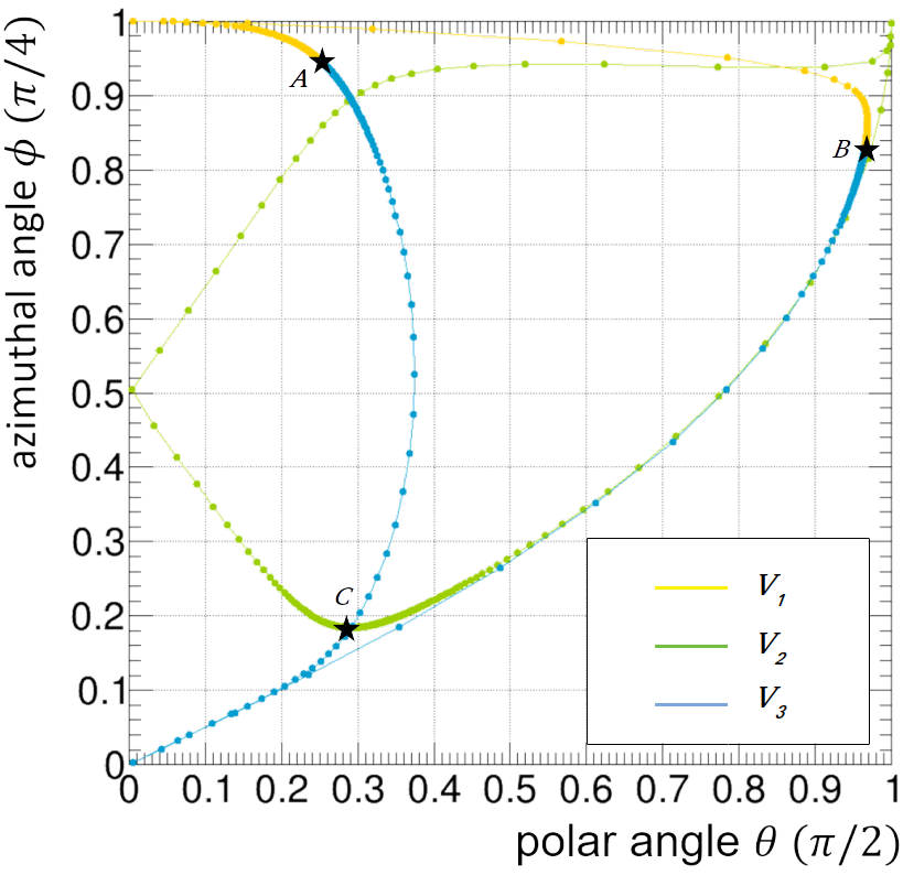
Figure 4: Spherical representation of $H(x)$’s eigenvectors. The eigenvectors $V_{1}$ (yellow), $V_{2}$ (green), and $V_{3}$ (blue). The starting point for each vector is $V_{1}=(0,1)$, $V_{2}=(1,1)$, and $V_{3}=(0,0)$. The dots represent equal steps in $x$, and help demonstrate the asymptotic behavior, when the density of points increase (meaning $x\rightarrow\infty$ (denoted by the three stars). The point $A=(0.25721,0.94092)$, corresponds to either $V_{1}$ when $x\rightarrow-\infty$ or $V_{3}$ when $x\rightarrow+\infty$. Similarly, $B=(0.96496,0.82418)$ is limit of $V_{1}$ when $x\rightarrow+\infty$ or $V_{3}$ when $x\rightarrow-\infty$. And finally, $C=(0.31152,0.18597)$ is the convergence of $V_{2}$ for both $x\rightarrow\pm\infty$.

One wishes to study the parametrized eigensystem of $H$, represented by $\{D,U\}$, as a function of $x$. By the definition in Eq.B.9, $D(x=0)=B$ therefore $U(x=0)=1$. In other words, at $x=0$ the eigenvalues of $H$ are not only the same as those of $B$, but they follow the same order. It is also possible to infer just from Eq. B.9 the behavior of $H$ when $x\rightarrow\pm\infty$, since $A\,x$ becomes the dominant term and the eigenvalues of $H$ assume the form of $x\ \lambda_{k}^{A}$. This means that the eigensystem of $H$ has an asymptotic behavior and, for instance, one might be tempted to write $\lambda_{1}^{H}(x)=x\ \lambda_{1}^{A}+\lambda_{1}^{B}$ in order to describe $\lambda_{1}^{H}(x)$ asymptote. However, there is no explicit information stating which $x\ \lambda_{k}^{A}$ corresponds to which $\lambda_{j}^{B}$. Unless $H$ is diagonalized, the true correspondence between the eigenvalues near zero and its value elsewhere is not clear yet, being implicitly determined by the parametrization. Besides, the same $\lambda^{H}$ can have different asymptotes for each limit.

By applying the Sequential Jacobi Diagonalization, described in Sec. 3 and 4, numerical representation of $D(x)$ and $U(x)$ can be calculated for a range of $x$ around the origin. Figure 3(a) shows the functions $\lambda_{j}^{H}(x)$ for a $|x|\geq 3$, which contain all of this system’s features. Their behavior is analogous to that of trains changing tracks. There are three asymptotes, of the form

$$f_{k} = x\ \lambda_{k}^{A}+a_{k},\ \ \mbox{k=1,2,3}\ ,$$ (B.13)

where $k$ indicates a particular eigenvalue of $A$, as defined in Eq.B.10 to Eq.B.12, and $a_{1}=2.04297$, $a_{2}=2.89648$ and $a_{3}=1.05859$ are constants, numerically obtained by the method. Each $\lambda_{j}^{H}(x)$ follows these asymptotes, changing allegiance every time they intersect. There are also three intersection points, in increasing order of $x^{\star}_{12}\geq x^{\star}_{13}\geq x^{\star}_{23}$, with numerical values shown in Tab. B.1.

Intersection between	$x^{\star}_{jk}$	$y^{\star}_{jk}$
$f_{1}$ and $f_{2}$	-0.22873	2.60814
$f_{1}$ and $f_{3}$	0.17327	1.61484
$f_{2}$ and $f_{3}$	0.94276	4.08503

Table B.1: Intersections between asymptotes. These are the values of $x$ where each eigenvalue changes allegiance to one of the system’s asymptotes.

The intersection are obtained by considering the $\lambda_{k}$ curves as hyperbolas, where their point of closest approach is where their derivatives are equal, which can be seen on Fig. 3(b). At last, it is possible to examine the three eigenvectors by taking their real spherical representation, i.e.,

$$\theta_{k}=\cos^{-1}\left(U_{3k}^{\star}\ U_{3k}\right)\ \mbox{\hskip 28.45274ptand\hskip 28.45274pt}\ \phi_{k}=\tan^{-1}\left(U_{2k}^{\star}\ U_{2k}\right)\ ,$$ (B.14)

where it is implicit that $\sum_{jk}U_{jk}^{\star}\ U_{jk}=1$. Although this projection is a limited representation, where $V_{k}=(\theta_{k},\phi_{k})$, with $\theta/(\pi/2)\in[0,1]$ and $\phi/(\pi/4)\in[0,1]$, it is enough to observe the their limiting behavior, as shown on Fig. 4.

The initial position of each vector is $V_{1}=(0,1)$, $V_{2}=(1,1)$, and $V_{3}=(0,0)$, when $x=0$, revolving around the unit sphere for other values of $x$. When we compare each eigenvector with its corresponding eigenvalue on Fig. 3(a), it is possible to correlate their behavior. For instance, how $V_{1}\rightarrow V_{3}$ as $x\rightarrow\pm\infty$ or how although $V_{2}$ crosses the other eigenvectors several times, the eigenvalues are never degenerate.

In conclusion, all the values and functions obtained in this example matches their analytical counterpart up to $10^{-14}$, which is the precision set for the method’s precision $\varepsilon$, while the expected precision for evaluating the analytical solutions is $10^{-15}$ (using 64-bit floats).

Appendix C Neutrino Physics Application

This section should exemplify to a neutrino physics how the Sequential Jacobi Diagonalization can be useful. In what follows, I will consider that the reader is familiar with the current mass-flavor mixing model, and the PMNS parametrization, limiting the exposition to some key points. The focus is the application of the previously proposed method. For neutrino physics enthusiasts, see Refs. [6, 16] and references therein for a review.

Parameter	Best fit	$1\sigma$ range	$3\sigma$ range
$\Delta m^{2}_{21}$ $\!/10^{-5}$	7.37	7.21 - 7.54	6.93 - 7.97
$\sin^{2}\theta_{12}$ $\!/10^{-1}$	2.97	2.81 - 3.14	2.50 - 3.54
Normal Hierarchy (NH)
$+\Delta m^{2}_{31}$ $\!/10^{-3}$	2.39	2.35 - 2.43	2.27 - 2.51
$\sin^{2}\theta_{13}$ $\!/10^{-2}$	2.14	2.05 - 2.25	1.85 - 2.46
$\sin^{2}\theta_{23}$ $\!/10^{-1}$	4.37	4.17 - 4.70	3.79 - 6.16
$\delta_{CP}/\pi$	1.35	1.13 - 1.64	0 - 2
Inverted Hierarchy (IH
$-\Delta m^{2}_{31}$ $\!/10^{-3}$	2.35	2.31 - 2.40	2.23 - 2.48
$\sin^{2}\theta_{13}$ $\!/10^{-2}$	2.18	2.06 - 2.27	1.86 - 2.48
$\sin^{2}\theta_{23}$ $\!/10^{-1}$	5.69	4.28 - 4.91	3.83 - 6.37
$\delta_{CP}/\pi$	1.32	1.07 - 1.67	0 - 2

Table C.1: Best fit values, $1\sigma$ and $3\sigma$ rages for the global fit of all relevant neutrino oscillation data[17]. Here, the notation used by the original reference is changed in favor of one that best suits this work.

Sequential Jacobi Diagonalization is of particular interest in the context of matter effects[4] in neutrino oscillations, also known as the Mikheyev-Smirnov-Wolfenstein (MSW) effect[2, 3]. In it, the presence an interacting medium shifts the energy levels of the Hamiltonian. This in turn leads to a new set of effective values for neutrino mixing parameters, either enhancing or suppressing the oscillation pattern, depending on certain conditions.

As the mass-flavor mixing model states[16], a three-neutrino system can be represented by a free Hamiltonian which is diagonal when expressed in the mass basis, $H_{m}=(\Delta m^{2}_{21}/2p)\times\mbox{diag}\left(0,1,\alpha\right)$, with $\alpha=\Delta m^{2}_{31}/\Delta m^{2}_{21}$ and the $\Delta m^{2}_{ij}$ are the squared-mass differences between the neutrino mass-states. The unitary mixing matrix $U$ takes the diagonal $H_{m}$ to the flavor basis via a similarity transformation,

$$H_{f}=U\ H_{m}\ U^{\dagger}\ ,$$ (C.1)

with $U$ being the result of three real rotations (with Euler angles $\theta_{12}$, $\theta_{23}$ and $\theta_{13}$) and at least one complex phase $\delta_{\mbox{\scriptsize CP}}$. In the presence of an interacting background, represented by a potential matrix $V$, the total Hamiltonian of the system becomes

$$\tilde{H}_{f}=U\ H_{m}\ U^{\dagger}+V\ ,$$ (C.2)

where the $\sim$ sign represents non-vacuum values, with $V$ being a general real matrix, encoding how each neutrino flavor interacts with the medium. The physical observables are those related to the neutrino oscillation pattern, namely the oscillation length and amplitudes, given by the eigenvalues and eigenvectors of $\tilde{H}_{f}$, respectively. Let $\tilde{U}$ be the diagonalizing transformation that realizes the following,

$$\tilde{H}_{m} = \tilde{U}^{\dagger}\ \tilde{H}_{f}\ \tilde{U}$$

$$= \tilde{U}^{\dagger}\ \left(U\ H_{m}\ U^{\dagger}+V\right)\tilde{U}$$

where $\tilde{H}_{m}\rightarrow H_{m}$, and $\tilde{U}\rightarrow U$, when $V\rightarrow 0$. Eq. C is equivalent to Eq.17, with $A=\tilde{H}_{f}$ and $D=\tilde{H}_{m}$. This single realization evokes the motivation behind this study, since while Eq.17 just the starting point of a diagonalization tool, Eq. C has actual meaning in neutrino physics. It can be overstated how convenient this matching is.

Let $\tilde{H}_{m}=(\Delta m^{2}_{21}/2p)\times\mbox{diag}\left(\lambda_{1},\lambda_{2},\lambda_{3}\right)$ be the diagonal form of $\tilde{H}_{f}$, with $\lambda_{k}$ the relevant factors of its eigenvalues. From the elements of the diagonalizing transformation of $U$ (or $\tilde{U}$) it is possible to define three Mixing Amplitudes,

$$\sin^{2}2\theta_{12}=4\frac{\left|U_{e1}\right|^{2}\,\left|U_{e2}\right|^{2}}{\left(1-\left|U_{e3}\right|^{2}\right)^{2}}\ ,\mbox{\hskip 28.45274pt}\ \sin^{2}2\theta_{23}=4\frac{\left|U_{\mu 1}\right|^{2}\,\left|U_{\tau 2}\right|^{2}}{\left(1-\left|U_{e3}\right|^{2}\right)^{2}}\ ,$$

and

$$\sin^{2}2\theta_{13} = 4\left|U_{e3}\right|^{2}\,\left(\left|U_{\mu 3}\right|^{2}+\left|U_{\tau 3}\right|^{2}\right)\,.$$ (C.4)

representing how the mass-eigenstates are mixed into the flavor states. This notation is corresponds to the PMNS parametrization[6]. It is also possible to isolate the effects of CP-violation, represented by the Jarlskog invariant,

$$J_{\mbox{\scriptsize CP}}=Im\left\{U_{\mu 3}\,U^{\star}_{\mu 2}\,U_{e2}\,U^{\star}_{e3}\right\}$$ (C.5)

where $J_{\mbox{\scriptsize CP}}$ represents the difference between neutrino and anti-neutrino oscillation.

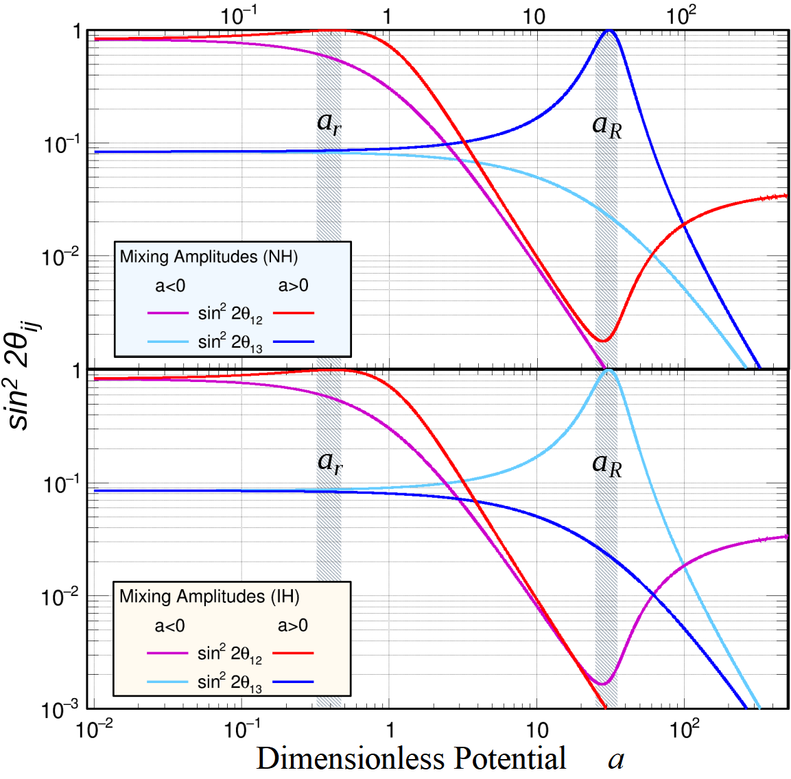
(a) Mixing Amplitudes, as a function of $|a|$.

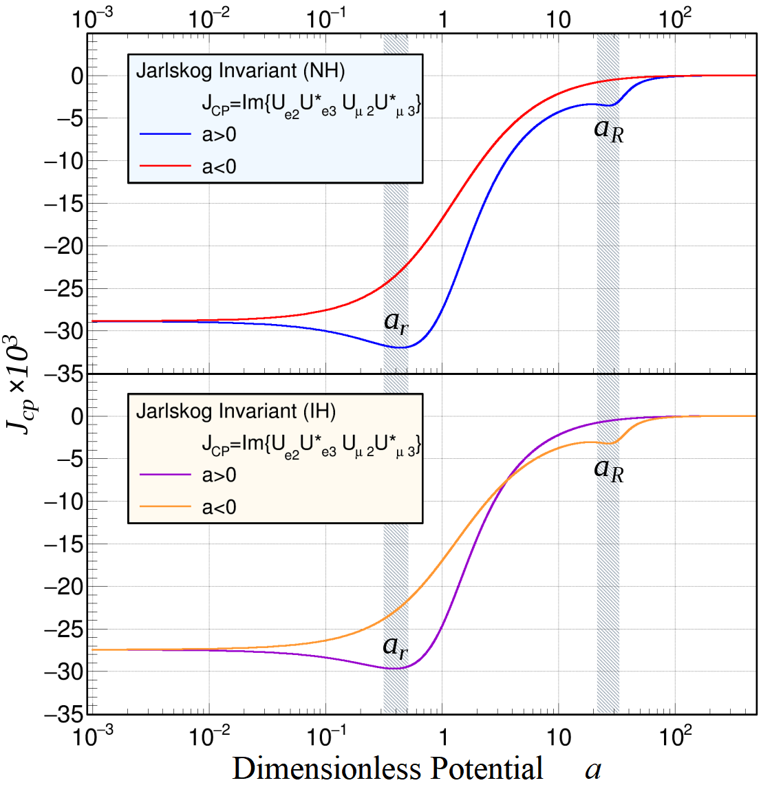
(b) Jarlskog Invariant, as a function of $|a|$.

Figure 5: (a) The matter-enhanced values of $\sin^{2}2\theta_{12}$ (blue if $a>0$ and cyan is $a<0$) and $\sin^{2}2\theta_{13}$ (red if $a>0$ and magenta is $a<0$) are shown for NH (top) and IH (bottom). (b) $J_{\mbox{\tiny CP}}$, as defined on Eq.C.5, using both NH (top) and IH (bottom) values (Tab C.1). For large $a$, $J_{\mbox{\tiny CP}}\rightarrow 0$, meaning that both neutrino and antineutrinos would show the same oscillation pattern.

Eqs. C.4 and C.5 will lead to different values, depending on the elements of the potential $V$. As an example, in non-standard interaction searches, the elements of $V$ can be either independent of each other or given by an underling model. In the case of an ordinary-matter background, however, the potential can be as simple as $V=(\Delta m^{2}_{21})/2p\times\mbox{diag}\left(a,0,0\right)$, with $a=2pV_{cc}/\Delta m^{2}_{21}$. Regardless, sequential diagonalization can be used to obtain the behavior of $\tilde{H}_{f}$’s eigensystem as a function of a specific model parameter or even the complete set of $V$ elements, which would be model-independent. In the case of a constant and uniform background, these definitions are enough to completely define the system. When this is not the case, it becomes necessary to also know how $\tilde{U}$ varies along the neutrino’s trajectory $x$, i.e.,

$$\frac{d\tilde{U}_{ij}}{dx}=\sum_{k\ell}\ \frac{dU_{ij}}{dV_{k\ell}}\ \frac{dV_{k\ell}}{dx}\ .$$ (C.6)

This is the point where the Sequential Jacobi Diagonalization can provide a worthy contribution. The values of ${d\tilde{U}_{ij}}/dx$ can be obtained prior to a full model analysis since it should be recalculated less frequently, if ever twice in a single study. Monte Carlo productions, as well as model fitting, can make use of a look-up table (LUT) instead of performing thousands of diagonalizations at every step. The more demanding simulations for the next generation of neutrino detectors, such as DUNE[9], can benefit from this approach.

In order to one concrete example, we can appreciate an application using only Standard Model physics, for which there are analytical solutions. In this case, the relevant matter potential is $V=\mbox{diag}\left(V_{cc},0,0\right)$, with $V_{cc}$ being the charged current potential between electrons in the medium and the electron-(anti)neutrino. Since global phases do not influence the final oscillation probabilities, we can place $\Delta m^{2}_{21}/2p$ in evidence, writing $V=\mbox{diag}\left(a,0,0\right)$, with $a=2pV_{cc}/\Delta m^{2}_{21}$. The parameter $a$ encodes all the background description such as density, interaction strength, and uniformity. By using Sequential Jacobi Diagonalization, it is possible to obtain all the relevant observables and still be agnostic with respect to the background properties, which can be added at a later point of the computation.

The total Hamiltonian to be diagonalized is $\tilde{H}_{m}(a)$, where $a>0$ means that both the neutrinos and the background are of the same nature, i.e., either both matter or both antimatter, while $a<0$ represents the matter/antimatter combination. Using the vacuum values on C.1, it is possible to obtain two distinct values for $\alpha$, $\alpha_{\mbox{\scriptsize NH}}=32.4$ and $\alpha_{{\mbox{\scriptsize IH}}}=-31.9$, corresponding to NH and IH, respectively. All results that follow will show four distinct cases: $\pm a$ and NH/IH.

The analytical solutions for the Mixing Amplitudes[7, 8] are compared to the Sequential Jacobi Diagonalization, being in agreement up to the chosen precision ($\varepsilon=10^{-14}$). Fig. 5(a) shows the mixing amplitudes $\sin^{2}2\theta_{12}$ and $\sin^{2}2\theta_{13}$ as a function of $|a|$ ($\sin^{2}2\theta_{23}$ is not shown since it is indistinguishable from 1 in this scale). It is possible to observe the resonant MSW effect, related to the two mass-scales. The lower resonance $a_{r}$ affects $\sin^{2}2\theta_{12}$, while the higher one $a_{R}$ affects $\sin^{2}2\theta_{13}$ and $\sin^{2}2\theta_{23}$. The latter is not shown on the plots since it would be indistinguishable from unit due to its large vacuum value.

On Fig. 6, we observe the eigenvalues of $H_{m}$ for NH and IH. The vacuum eigenvalues are $\lambda_{1}=0$, $\lambda_{2}=1$, and $\lambda_{3}=\alpha$, and it is possible to see that resonances $a_{r}$ and $a_{R}$ represent the points where the eigenvalues change asymptotes.

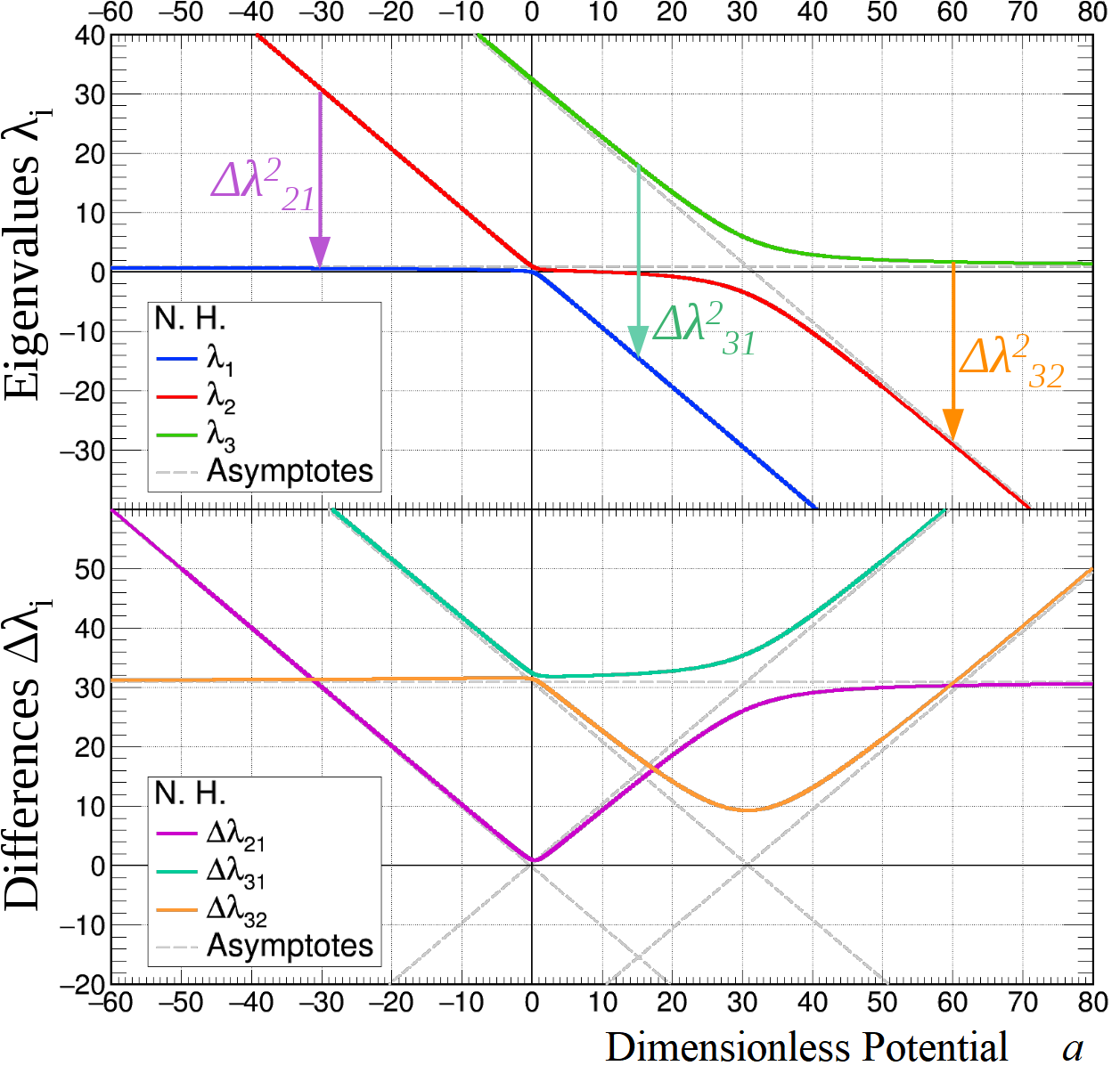
(a) Eigenvalues of $\tilde{H}_{m}$ for NH.

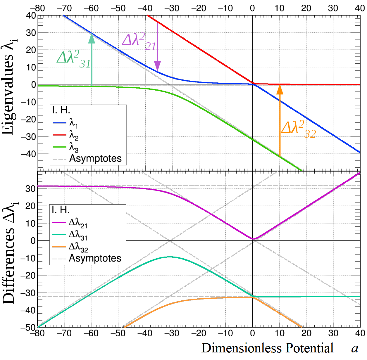
(b) Eigenvalues of $\tilde{H}_{m}$ for IH.

Figure 6: Eigenvalues of $\tilde{H}_{m}$ (Eq.C), for NH (a) and IH (b). Each individual eigenvalue $\lambda_{i}$ is drawn as a function of the dimensionless background descriptor $a$, representing the MSW effect in ordinary matter. The differences $\Delta\lambda_{ij}$ are also shown, since they correlate to the oscillation length. All vacuum values are taken from (Tab C.1).

Finally, Fig. 5(b) shows how the Jarskog invariant is affected by the background. Regardless of the hierarchy case, $a_{r}$ represents a resonant minimum for $a>0$, and $a>a_{R}$ will always lead to $J_{\mbox{\scriptsize CP}}=0$, meaning that neutrinos and antineutrinos would behave the same. It is worth noting that the existence of CP-violation in neutrino oscillations is not confirmed and the results shown here only consider the best fit values for $\delta_{\mbox{\scriptsize CP}}$, which is still compatible with zero. No matter what the true $\delta_{\mbox{\scriptsize CP}}$ is, it affects $J_{\mbox{\scriptsize CP}}$ with all the previous observables remaining unchanged.

References

- Hubbard et al. [2001] J. Hubbard, D. Schleicher, and S. Sutherland. How to find all roots of complex polynomials by newton’s method. Invent. math., 146:1–33, 2001. doi: 10.1007/s002220100149. URL https://doi.org/10.1007/s002220100149.
- Wolfenstein [1978] L. Wolfenstein. Neutrino oscillations in matter. Phys. Rev. D, 17:2369–2374, May 1978. doi: 10.1103/PhysRevD.17.2369.
- Mikheev and Smirnov [1985] S. P. Mikheev and A. Yu. Smirnov. Resonance Amplification of Oscillations in Matter and Spectroscopy of Solar Neutrinos. Sov. J. Nucl. Phys., 42:913–917, 1985. [Yad. Fiz.42,1441(1985)].
- Blennow and Yu. Smirnov [2013] Mattias Blennow and Alexei Yu. Smirnov. Neutrino propagation in matter. Advances in High Energy Physics, 2013(Article ID 972485):33, 2013. doi: 10.1155/2013/972485.
- Maltoni, Michele and Yu. Smirnov, Alexei [2016] Maltoni, Michele and Yu. Smirnov, Alexei. Solar neutrinos and neutrino physics. Eur. Phys. J. A, 52(4):87, 2016. doi: 10.1140/epja/i2016-16087-0.
- Smirnov [2016] A. Yu. Smirnov. Solar neutrinos: Oscillations or No-oscillations? . arXiv, 2016.
- Zaglauer and Schwarzer [1988] H. W. Zaglauer and K. H. Schwarzer. The mixing angles in matter for three generations of neutrinos and the msw mechanism. Zeitschrift für Physik C Particles and Fields, 40(2):273–282, Jun 1988. ISSN 1431-5858. doi: 10.1007/BF01555889.
- Kimura et al. [2002] Keiichi Kimura, Akira Takamura, and Hidekazu Yokomakura. Exact formulas and simple dependence of neutrino oscillation probabilities in matter with constant density. Phys. Rev. D, 66:073005, Oct 2002. doi: 10.1103/PhysRevD.66.073005.
- Abi et al. [2020] B. Abi, R. Acciarri, M. A. Acero, et al. Long-baseline neutrino oscillation physics potential of the dune experiment. Eur. Phys. J. C, 80(978), 2020. doi: 10.1140/epjc/s10052-020-08456-z.
- Jacobi [1846] C. G. J. Jacobi. über ein leichtes verfahren, die in der theorie der säkularstörungen vorkommenden gleichungen numerisch aufzulösen. Journal für die reine und angewandte Mathematik, pages 51–94, 1846.
- Eberlein [1962] P. J. Eberlein. A jacobi-like method for the automatic computation of eigenvalues and eigenvectors of an arbitrary matrix. Journal of the Society for Industrial and Applied Mathematics, 10(1):74–88, 1962. ISSN 0368-4245. doi: 10.1137/0110007.
- Hansen [1963] E. R. Hansen. On cyclic jacobi methods. Journal of the Society for Industrial and Applied Mathematics, 11(2), 448–459. (12 pages), 11(2):448–459, 1963. ISSN 0368-4245. doi: 10.1137/0111032.
- Press et al. [1992] William H. Press, Saul A. Teukolsky, William T. Vetterling, and Brian P. Flannery. Numerical Recipes in C. Cambridge University Press, Cambridge, USA, second edition, 1992.
- Forsythe and Henrici [1960] G. E. Forsythe and P. Henrici. The cyclic jacobi method for computing the principal values of a complex matrix. Trans. Am. Math. Sot., 94:1 – 23, 1960. ISSN 0002-9947. doi: 10.1090/S0002-9947-1960-0109825-2.
- Nazareth [1975] Larry Nazareth. On the convergence of the cyclic jacobi method. Linear Algebra and its Applications, 12(2):151 – 164, 1975. ISSN 0024-3795. doi: 10.1016/0024-3795(75)90063-4.
- Bilenky [2014] S. M. Bilenky. Neutrino oscillations: brief history and present status . arXiv, 2014.
- Capozzi et al. [2016] F. Capozzi, E. Lisi, A. Marrone, D. Montanino, and A. Palazzo. Neutrino masses and mixings: Status of known and unknown 3 parameters. Nuclear Physics B, 908:218 – 234, 2016. ISSN 0550-3213. doi: 10.1016/j.nuclphysb.2016.02.016. Neutrino Oscillations: Celebrating the Nobel Prize in Physics 2015.