Solving the Electrical Impedance Tomography Problem with a DeepONet Type Neural Network: Theory and Application

Abstract

In this work, we consider the non-invasive medical imaging modality of Electrical Impedance Tomography, where the problem is to recover the conductivity in a medium from a set of data that arises out of a current-to-voltage map (Neumann-to-Dirichlet operator) defined on the boundary of the medium. We formulate this inverse problem as an operator-learning problem where the goal is to learn the implicitly defined operator-to-function map between the space of Neumann-to-Dirichlet operators to the space of admissible conductivities. Subsequently, we use an operator-learning architecture, popularly called DeepONets, to learn this operator-to-function map. Thus far, most of the operator learning architectures have been implemented to learn operators between function spaces. In this work, we generalize the earlier works and use a DeepONet to actually learn an operator-to-function map. We provide a Universal Approximation Theorem type result which guarantees that this implicitly defined operator-to-function map between the the space of Neumann-to-Dirichlet operator to the space of conductivity function can be approximated to an arbitrary degree using such a DeepONet. Furthermore, we provide a computational implementation of our proposed approach and compare it against a standard baseline. We show that the proposed approach achieves good reconstructions and outperforms the baseline method in our experiments.

1 Introduction

In recent years tremendous progress has been made in developing accurate, non-invasive medical imaging techniques for disease detection and diagnosis and to make it suitable for practical deployment. One such medical imaging technology is Electrical Impedance Tomography (EIT). EIT is a functional imaging technique that seeks to reconstruct the spatial conductivity within a domain by applying currents and measuring voltages across electrodes attached to the boundary of the domain of interest. EIT has been shown to be clinically useful in monitoring lung function and breast cancer, see e.g. [14, 19]. It is now becoming an increasingly promising neuro-imaging method, e.g. in early detection of cerebral edema and monitoring the effect of mannitol dehydration, [72]. It is also being used in epilepsy imaging to detect seizure onset zones, [71]. Moreover, a bedside EIT stroke monitoring system has been developed for clinical practice and there is growing consensus among practitioners for utilizing EIT in multi-modal imaging for diagnosing and classifying strokes, see e.g.[2, 61]. In spite of the fact that EIT has lower spatial resolution than some other tomographic techniques such as computed tomography and MRI, it has relatively fast data acquisition times, relatively inexpensive hardware and does not use ionizing radiations, making it a versatile and safer alternative to many other medical imaging modalities, see [36] and the references therein.

Recall that a typical EIT experiment consists of injecting a weak excitation current through boundary electrodes surrounding the region of interest and imaging the distribution of electrical parameters in the region of interest by measuring voltage signals on such electrodes. Thus the measured data arises as a current-to-voltage map, which is physically related to the internal conductivity in the region of interest. Different kinds of tissues can be differentiated based on their different conductivity values, which may also be altered in diseased states. As such, the inverse problem consists of detecting physiological and pathological changes in the conductivity profile based on measurements of the current-to-voltage map across the boundary electrodes. More recently, there is a growing interest among theoreticians and practitioners alike in exploiting various machine-learning based algorithms and neural-network architectures to solve the EIT inverse problem. In this work, we use a DeepONet architecture and provide approximation-theoretic guarantees which show that by increasing the number of electrodes and by appropriately choosing the number of network parameters, one can estimate the internal conductivity to any arbitrary precision in a suitable norm. Furthermore, we implement such an architecture based on the theoretical DeepONet framework and compare its performance against a standard baseline to show that the propose neural-network outperforms that state-of-the-art baseline in our numerical experiments.

For the benefit of the readers, in the following subsections we will first give a self-contained mathematical description of the inverse problem at hand and survey some related literature. In the subsequent sections, we will describe our main theoretical results, give details about the proposed architecture and support our findings with numerical experiments. We begin now by summarizing our main contributions.

1.1 Contribution

Our contributions can be summarized in the following points:

• In this work, we propose a DeepONet architecture for solving the EIT inverse problem and provide a rigorous mathematical justification for using such an architecture.

• Various approximation-theoretic results for operator networks which seek to learn operators between infinite-dimensional function spaces have appeared in the recent past. We extend those results in order to make them suitable for the EIT inverse problem by proving a Universal Approximation Theorem type result for the case when the input space lies in the class of Hilbert-Schmidt operators (related to the current-to-voltage map) and the output space is a function space (corresponding to the conductivity function).

• We show that our proposed method achieves good reconstructions and show that it outperforms the state-of-the-art IRGN baseline.

1.2 Mathematical preliminaries and background of the EIT problem

We will begin by introducing the notation used in this work: Let $\Omega\subset\mathbb{R}^{d}$ for $d\geq 2$ be some simply connected domain with smooth boundary and $\Omega^{\prime}\subset\Omega$ be a compact set. We denote the set of essentially (i.e. almost surely) bounded functions by $L^{\infty}(\Omega)$ and the subset of essentially positive functions by $L^{\infty}_{+}(\Omega).$ In general $H^{s}(X)$ will be used to refer to the space of $L^{2}-$ Sobolev space of functions on some smooth bounded domain $X$. Additionally, $H^{1}_{\diamond}(X)$ and $L^{2}_{\diamond}(X)$ will be used to denote the spaces of $H^{1}$ and $L^{2}$ functions with vanishing integral mean on the boundary $\partial X$, i.e. $h\in H^{1}_{\diamond}(\Omega):=\{h\in L^{2}(X):\int_{\partial X}hdS=0\}$ and similarly, $g\in L^{2}_{\diamond}(X):=\{g\in L^{2}(X):\int_{\partial X}gdS=0\}$. We will also denote the space of Linear operators from $X$ to $Y$ by, $\mathcal{L}(X\to Y)$. Mathematically, the problem can be formulated as recovery of the conductivity function $\sigma(x)$ in some simply connected domain $\Omega$ based on electric potential and current measurements made entirely on the boundary $\partial\Omega$ (or, some subset of it $\Sigma\subset\partial\Omega$). To formulate the problem consider the following elliptic partial differential equation with associated Neumann boundary-data which serves as a model for EIT:

$$\nabla\cdot(\gamma\nabla u) =0\quad\mbox{ in }\Omega;$$ (1)

$$\begin{split}\gamma\partial_{\nu}u|_{\partial\Omega}&=g\mbox{ on }\partial\Omega\quad(\text{or more generally }\Sigma)\\ &=0\mbox{ else.}\end{split}$$ (2)

Here $\gamma\in L^{\infty}_{+}(\Omega)$ is the internal conductivity in the medium $\Omega$ such that $\gamma=1\mbox{ in }\Omega\setminus\Omega^{\prime}$, and $u(x)$ is the electric potential in the interior. Loosely speaking, we will refer to $\gamma\equiv 1$ as the background conductivity. The Neumann boundary-data models the applied current. In the abstract continuum model (CM), the corresponding boundary measurements of the voltage (Dirichlet data) are given by the Neumann-to-Dirichlet (N-t-D) operator defined on the boundary $\partial\Omega$ ( or more generally on a subset $\Sigma\subset\partial\Omega$):

$$\Lambda_{\gamma}:L^{2}_{\diamond}(\partial\Omega)\to L^{2}_{\diamond}(\partial\Omega),\quad g\mapsto u|_{\partial\Omega}.$$ (3)

To emphasize, $u|_{\partial\Omega}$ refer to the voltage measurements on the the boundary $\partial\Omega$. Additionally, here and below we will use $\Lambda_{1}$ to denote the background N-t-D operator corresponding to the background conductivity. The abstract model as described in this article is also called the Calderón problem and has been studied by many authors since it was first described in [9]. We would like to mention here, that in the abstract mathematical formulation, typically the Dirichlet-to-Neumann (D-t-N) map is considered instead of the N-t-D map as is considered in this work. However, in practical settings such as in EIT, the data that is generated is in the form of current-to-voltage maps which is best captured by the N-t-D maps. A more practical formulation of the EIT problem is given by the Complete Electrode Model (CEM), [17]. As before we let $\gamma\in L^{\infty}_{+}(\Omega)$. Let there be $M$ open, connected and mutually disjoint electrodes, $E_{m}\subset\partial\Omega$, $m=\{1,\cdots,M\}$ having the same contact impedance $z>0$. Assuming that the injected currents $I_{m}$ on the electrodes satisfy the Kirchoff condition, i.e. $\Sigma_{m=1}^{M}I_{m}=0$, the resulting electric potential $(u,U)\in H^{1}(\Omega)\times\mathbb{R}^{M}$ satisfies (1) along with the following conditions on the boundary:

$$\gamma\partial_{\nu}u =0;\quad\text{on }\partial\Omega\setminus\bigcup E_{m}$$ (4)

$$\int_{E_{m}}\gamma\partial_{\nu}udS =I_{m}\quad\text{on }E_{m},m=1,\cdots,M$$ (5)

$$u+z\sigma\partial_{\nu}u =U_{m}\quad\text{on }E_{m},m=\{1,\cdots,M\}$$ (6)

where the vector $U=(U_{1},\cdots,U_{M})$ represents voltage measurement on the electrodes satisfying a ground condition $\Sigma_{m=1}^{M}U_{m}=0$. We can thus define the $M-$electrode current to voltage operator, $R_{M}(\gamma):\mathbb{R}^{M}_{\diamond}\to\mathbb{R}^{M}_{\diamond}:I:=(I_{1},\cdots,I_{M})\mapsto(U_{1},\cdots,U_{M})=U$ and $U=R_{M}(\gamma)I$. For later use, we also define the ‘shifted’ CEM operator, $\tilde{R}_{M}(\gamma):={R}_{M}(\gamma)-{R}_{M}(1)$ where $\tilde{R}_{M}(1)$ is the background CEM current-to-voltage operator. Since the background operator $\tilde{R}_{M}(1)$ is known, $\tilde{R}_{M}(\gamma)$ is completely determined by $R_{M}(\gamma)$ and vice-versa. Before we define the inverse problem at hand, we will first define the set of admissible conductivities considered in this work. We recall the following definition from [27, Definition 2.2].

Definition 1.

A set $\mathcal{F}\subset L^{\infty}{(\Omega)}\cap L^{2}(\Omega)$ is called a finite dimensional subset of piecewise analytic functions if its linear span

$$\mathrm{span}\ \mathcal{F}=\bigg{\{}\sum\limits_{j=1}^{k}\lambda_{j}f_{j}:k\in\mathbb{N},\lambda_{j}\in\mathbb{R},f_{j}\in\mathcal{F}\bigg{\}}\subset L^{\infty}(\Omega)\cap L^{2}(\Omega)$$

contains only piecewise analytic function and $\mathrm{dim}\ (\mathrm{span}\ \mathcal{F})<\infty.$

Given such a finite dimesnional subset $\mathcal{F}$ and two numbers $m,M$ we denote the space of admissible conductivities $\Gamma$ as:

$$\Gamma =\{\gamma\in\mathcal{F}:M>\gamma(x)\geq m>0,\gamma(x)=1\text{ in }\Omega\setminus\Omega^{\prime}\}$$ (7)

As $\Omega$ is bounded, any such admissible conductivity is clearly contained in $L^{2}(\Omega).$ Furthermore, $\Gamma$ is closed by virtue of being a known finite dimensional subspace of $L^{\infty}(\Omega)\cap L^{2}(\Omega)$. Such conductivities have been considered in the literature before, see e.g. [27, 21] The inverse problem in CM can then be stated as, given all possible pairs of associated functions $(g,u|_{\Sigma})$, we want to find $\gamma\in\Gamma$.

1.3 Related Research

An EIT experiment applies the electrical current (Neumann data) on $\partial\Omega$ to measure the electrical potential differences on $\partial\Omega$. By doing so, the so-called Neumann-to-Dirichlet (NtD) operator $\Lambda_{\sigma}$ is obtained. The inverse problem is reconstructing the unknown conductivity $\sigma$ from a set of EIT experiments [7, 13, 25, 48]. Early important results by Sylvester and Uhlmann [69], and by Nachmann [54] established that unique recovery of the conductivity from the boundary data in the form of D-t-N map is possible in the (abstract) Calderón problem set-up. Stability estimates for the Calderón problem were given in [4, 56]. Optimality of such stability estimates, at least up to the order of the exponents, was proved in [51]. [64, 70] and many references therein contain an exhaustive survey of results in this area.

EIT is a highly nonlinear and strongly ill-posed problem. Therefore, in the classical literature, EIT requires a regularization for a good reconstruction [32, 33]. In the literature, there are abundant approaches for solving the EIT inverse problem including the factorization method [38], d-bar method [31], or variational methods for least-square fitting [32, 33, 3, 37] as well as, on statistical methods [1, 3, 34, 67].

There is also some recent research on deep learning for solving the EIT inverse problem. They include using Physics inspired neural networks [60], different kinds of convolutional neural networks [24, 18, 23], and shape reconstruction [68]. On the other hand, an architecture called Deep-Operator-Networks (DeepONet, or DON) was proposed in [50] for learning implicitly defined operator maps between infinite-dimensional function spaces. This architecture was a massive generalization of an earlier known (shallow) operator-network architecture proposed in [12], see also [10, 11]. Subsequently, variations of DeepONet (more generally, neural-operators) have been used for solving important physical problems and substantial efforts have been made to understand the theoretical underpinnings of why this approach seems to be particularly efficient, see e.g. [74, 28, 65, 59, 8, 35, 46, 62, 22, 6, 47, 41, 15, 40, 45, 39] and the many references therein. The main idea in operator-learning is that it seeks to directly approximate the operator map between infinite-dimensional spaces and in many cases can be shown to approximate any continuous operator to desired accuracy. Hereby, we do not have the disadvantages of the somewhat limited resolution of traditional convolutional neural-network based methods such as [24, 18, 23]. While most of the work in the literature has so far appeared in approximating a map between two function spaces, in EIT, we are interesting in learning the map between a space of (N-t-D) operators to a space of (conductivity) functions. Furthermore, we do not only provide strong experimental results for the DeepONet implementation for EIT but also provide approximation-theoretic guarantees as a theoretical justification for this approach.

In the computer-vision community, a similar DeepONet based architecture was introduced as implicit-neural-networks or, INNs. The idea here is to replace conventional discretized signal representation with implicit representations of 3D objects via neural networks. In discrete representations images are represented as discrete grids of pixels, audio signals are represented as discrete samples of amplitudes, and 3D shapes are usually parameterized as grids of voxels, point clouds, or meshes. In contrast, Implicit Neural Representations seek to represent a signal as a continuous function that maps the domain of the signal (i.e., a coordinate, such as a pixel coordinate for an image) to the value of the continuous signal at that coordinate (for an image, an R,G,B color). Some early work in this field includes single-image 3D reconstructions [52, 29, 66], representing texture on 3D objects [57], representing surface light fields in 3D [58], or 3D reconstructions from many images [53]. Both DeepONets and INNs seek to learn implicitly defined continuous maps between the input and output spaces and thus share many similarities. Motivated by these works, one of the authors of this article used such network architectures for shape reconstruction in the EIT problem [68].

2 The Learning Problem for EIT

Our goal in this article is to propose a DeepONet based neural-network architecture for learning to invert Neumann-to-Dirichlet operator relevant to the problem of EIT. To formally set up the learning problem, let us consider the shifted abstract N-t-D operator $\tilde{\Lambda}_{\gamma}={\Lambda}_{\gamma}-\Lambda_{1}$, where $\Lambda_{1}$ is the background N-t-D operator. Analogous to the CEM case, $\tilde{\Lambda}_{\gamma}$ is completely dtermined by $\Lambda_{\gamma}$ and vice-versa. Now we list some mapping properties of the operator $\tilde{\Lambda}_{\gamma}$ which will be crucial in our analysis. First of all, note that $\tilde{\Lambda}_{\gamma}$ is a smoothing opertor, see e.g. [30, Theorem A.3] and [20, (2.5)]. In particular the operator norm of $\tilde{\Lambda}_{\gamma}$ is bounded, i.e., $\lvert\lvert\tilde{\Lambda}_{\gamma}\rvert\rvert_{\mathcal{L}(H^{s}\to H^{t})}\leq C$ for all $s,t\in\mathbb{R}$. From [1, Lemma 18], we know that $\tilde{\Lambda}_{\gamma}\in\mathbb{H}_{r}$ for any $r$. Here $\mathbb{H}_{r}$ denotes a space of Hilbert-Schmidt operators, see [1, eq.10] which is a Hilbert-space in its own right. Consider the set $D_{\Lambda}=\{\tilde{\Lambda}_{\gamma}:\gamma\in\Gamma\}$ of N-t-D operators corresponding to admissible conductivities. We show in 3 that $D_{\Lambda}$ is a compact set of $\mathbb{H}_{r}$.

Formally, the problem is to ‘learn’ the map $G^{\text{true}}:D_{\Lambda}\to\Gamma$. More particularly, we want to design a deep neural network (DeepONet) to approximate the map, $G^{\text{true}}$. For learning operators between infinite dimensional spaces, DeepONets were introduced in [50, 43]. These generalized the (shallow-net) architecture proposed in [12, 11]. Theoretical guarantees for DeepONets were given in [43] where the neural network tries to learn operators between two Hilbert spaces. This theory was further generalized in [39, 42] and an architecture called Fourier Neural Operators was introduced for learning operators between Banach spaces having a certain approximation property. With this background in mind, and to set the stage for formulating our learning problem as learning an operator between two Hilbert Spaces, let us introduce a (regular)‘link function’ $\Phi:\mathbb{R}\to[m,\infty)$ such that any conductivity $\gamma\in\Gamma$ is given by $\gamma=\Phi\circ f$ for some $f\in L^{\infty}(\Omega)\cap L^{2}{(\Omega)}:=\tilde{\Gamma}$. An example of such a link function is given in [55, Example 8]. Now we will modify our operator learning problem. For this we first define a map, $\mathcal{G}^{\dagger}:D_{\Lambda}\to\tilde{\Gamma}$ where $\mathcal{G}^{\dagger}=\phi^{-1}\circ G^{\text{true}}$. Thus knowing $\mathcal{G}^{\dagger}$ completely determines $G^{\text{true}}$. Next we extend this map: Let $\mathcal{G}^{\dagger}:D_{\Lambda}\to L^{\infty}(\Omega)\cap L^{2}(\Omega)$ be the map as above, then there exists an extension $\mathcal{G}^{\dagger}_{\text{ext}}:\mathbb{H}_{r}\to L^{\infty}(\Omega)\cap L^{2}(\Omega)$ such that $\mathcal{G}^{\dagger}_{\text{ext}}|_{D_{\Lambda}}=\mathcal{G}^{\dagger}$. The extension $\mathcal{G}^{\dagger}_{\text{ext}}$ exists by Lemma 4. The map $\mathcal{G}^{\dagger}_{\text{ext}}$ will be approximated by a deep neural operator called DeepONet. Essentially, a neural operator is a parametric map between the input space (e.g. space of N-t-D operators) and the output space (e.g. space of admissible conductivities) that can be interpreted as a composition of three maps, an encoder, an approximator and a reconstructor, see [43] and Figure 1. As such an upper bound on the error in approximating the true operator by a neural operator can be split into upper bounds on the encoder error, the approximator error and the reconstructor error correspondingly. Now we recall the DeepONet as proposed in [43, 50] and adapt the definitions as applicable to the case of EIT. To that end, we define the following operators while keeping the terminology the same as in [43]:

Figure 1: The true map $\mathcal{G}^{\dagger}_{\text{ext}}$ is approximated by a composition of three maps, encoder $\mathcal{E}$, approximator $\mathcal{A}$ and reconstructor $\mathcal{R}$. The resultant error in the approximation thus comprises of encoder, approximator, and reconstructor errors.

• Encoder: Given a set of $M$ electrodes covering the boundary of the domain, $E_{m}\subset\partial\Omega$, $m=\{1,\cdots,M\}$ we define the encoder:

  $$\mathcal{E}_{M}:=\mathcal{E}:D_{\Lambda}\subset\mathbb{H}_{r}\to\mathbb{R}^{M}\times\mathbb{R}^{M};\quad\tilde{\Lambda}_{\gamma}\mapsto\tilde{R}_{M}(\gamma)$$ (8)

  The encoder can be thought of as ‘sensor evaluations’ in the spirit of [43]. Whenever it is clear from context, we will denote $\mathcal{E}_{M}$ by $\mathcal{E}$. As shown in subsection 7.1, the map $\mathcal{E}$ is continuous and can be extended continuously on $\mathbb{H}_{r}$. With a slight abuse of notation, we call this extended map $\mathcal{E}$ too.

• Decoder: While the encoder is a projection of an infinite-dimensional object (i.e. $\tilde{\Lambda}_{\gamma}\in\mathbb{H}_{r}$) into a finite-dimensional space, a decoder lifts back a finite dimensional object into its corresponding representation in the space of Hilbert-Schmidt operators. This lifting is done using the construction given in [20, section 6] and results in an operator ${\Lambda}^{M}_{\gamma}$, see [20, eqn. 6.8]. Thus, we have:

  $$\mathcal{D}_{M}:=\mathcal{D}:\mathbb{R}^{M}\times\mathbb{R}^{M}\to\mathbb{H}_{r};\quad\tilde{R}_{M}(\gamma)\mapsto\tilde{\Lambda}^{M}_{\gamma}.$$ (9)

  Similar to above, whenever it is clear from context, we will use the shorthand notation $\mathcal{D}$ instead of $\mathcal{D}_{M}$. Note that, $\mathcal{D}\circ\mathcal{E}(\tilde{\Lambda}_{\gamma})=\tilde{\Lambda}^{M}_{\gamma}.$ In particular, we use here as the decoder the construction outlined in [5, Section 3]. Indeed, given any Neumann data $f\in L^{2}_{\diamond}(\partial\Omega)$, $\tilde{\Lambda}^{M}_{\gamma}f:=\tilde{R}_{M}\tilde{P}^{E}_{M}{f}$ where the map $\tilde{P}^{E}_{M}$ is a (auxiliary) projection operator defined in accordance with [5, eq. (5.1)].

• Approximator: The approximator is a deep (feedforward) neural network defined as:

  $$\mathcal{A}:\mathbb{R}^{M}\times\mathbb{R}^{M}\to\mathbb{R}^{P};\quad\tilde{R}_{M}(\gamma)\mapsto\{\mathcal{A}_{k}\}_{k=1}^{P}$$ (10)

  The composition of encoder and approximator, i.e. $\beta:=\mathcal{A}\circ\mathcal{E}:\mathbb{H}^{r}\to\mathbb{R}^{P}$ will be referred to as the branch net.

• Reconstructor: Following [43], we denote a trunk-net:

  $$\mathbf{\tau}:\mathbb{R}^{d}\to\mathbb{R}^{P+1},\quad y=(y_{1},\cdots,y_{d})\mapsto\{\tau_{k}\}_{k=0}^{P}$$ (11)

  where each $\tau_{k}$ is a feed-forward neural net. This can be thought of as a point-encoder which encodes a point $y\in\mathbb{R}^{d}$ into a $P+1$ dimensional representation. Subsequently we denote a $\mathbf{\tau}$-induced reconstructor:

  $$\mathcal{R}_{P}:=\mathcal{R}:\mathbb{R}^{P}\to L^{2}(\Omega),\quad\mathcal{R}(\alpha_{k}):=\tau_{0}(y)+\Sigma_{k=1}^{P}\alpha_{k}\tau_{k}(y).$$ (12)

• Projector: Given a reconstructor $\mathcal{R}$ as above with $\tau_{k}\in L^{2}(\Omega);k=0,\cdots,P$ and $\{\tau_{k}\}_{k=1}^{P}$ as linearly independent we can define a projector:

  $$\mathcal{P}_{P}:=\mathcal{P}:L^{2}(\Omega)\to\mathbb{R}^{p},\quad\mathcal{P}(f)=\left(\langle f-\tau_{0},\tau_{1}^{*}\rangle,\cdots,\langle f-\tau_{0},\tau_{P}^{*}\rangle\right)$$ (13)

  where $\tau_{1}^{*},\cdots,\tau_{P}^{*}$ denotes the dual basis of $\tau_{1},\cdots,\tau_{p}$ such that:

  $$\langle\tau_{k},\tau_{l}^{*}\rangle=\delta_{kl}\quad\forall\text{ }k,l\in\{1,\cdots,P\}.$$

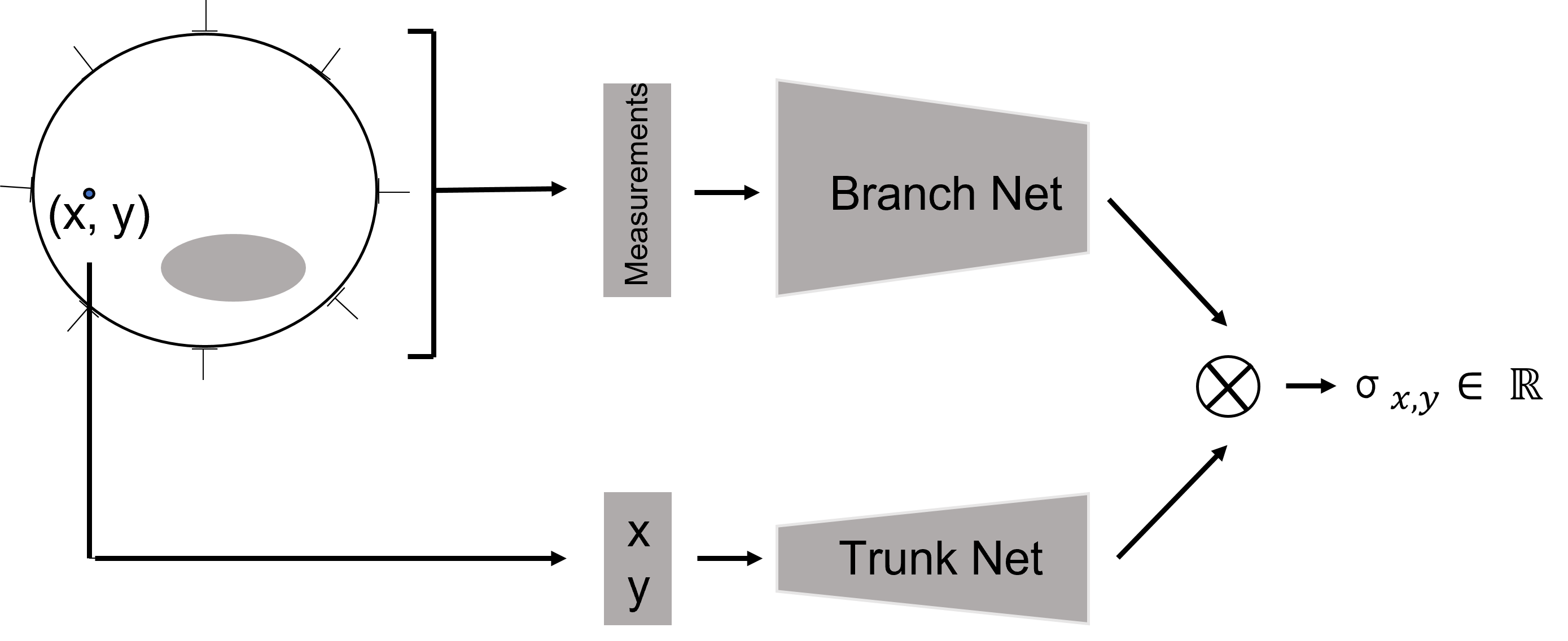
Figure 2: DeepONet architecture used in this manuscript. It feeds the EIT measurements into a Branch Net and 2d point on $\Omega$ into a Trunk Net. The outputs of both networks are combined via an inner product to predict the $\sigma_{x,y}$ at points $(x,y)$.

3 Main Approximation Theorem

The quality of the approximation will be determined by the extent to which these maps commute. The neural operator $\mathcal{G}_{\theta}$ will approximate the ‘true map’ $\mathcal{G}^{\dagger}_{\text{ext}}$. Recall that we denote encoding (by sensor evaluations) by $\mathcal{E}$, decoding by $\mathcal{D}$, Reconstructor map by $\mathcal{R}$, the projector map by $\mathcal{P}$, and the approximator map between finite dimensional spaces as $\mathcal{A}$. Referring to Fig. 1, notice that our neural operator will have the form $\mathcal{G}_{\theta}=\mathcal{R}\circ\mathcal{A}\circ\mathcal{E}$. Our goal is to find an upper bound on the error incurred in approximating $\mathcal{G}^{\dagger}_{\text{ext}}$ by $\mathcal{R}\circ\mathcal{A}\circ\mathcal{E}:=\mathcal{G}_{\theta}$ over the space of shifted N-t-D operators corresponding to admissible conductivities. More particularly we will prove the following theorem.

Theorem 1.

Consider the sets $\mathbb{H}_{r},D_{\Lambda}$, $\tilde{\Gamma}$, and $\mathcal{G}^{\dagger}_{\text{ext}}$ as above. Note $D_{\Lambda}$ is a compact set of $\mathbb{H}_{r}$. We will show that $\forall\epsilon>0$, there exist numbers $M\text{ and }P$ and continuous maps $\mathcal{E}:\mathbb{H}_{r}\to\mathbb{R}^{M}\times\mathbb{R}^{M}$, $\mathcal{R}:\mathbb{R}^{P}\to\tilde{\Gamma}$ and $\mathcal{A}:\mathbb{R}^{M}\times\mathbb{R}^{M}\to\mathbb{R}^{P}$ such that:

$$\sup\limits_{\tilde{\Lambda}_{\gamma}\in D_{\Lambda}}\lvert\lvert\mathcal{G}^{\dagger}_{\text{ext}}(\tilde{\Lambda}_{\gamma})-\mathcal{R}\circ\mathcal{A}\circ\mathcal{E}(\tilde{\Lambda}_{\gamma})\rvert\rvert_{L^{2}}\leq\epsilon$$ (14)

Proof.

The error term can be split in the following way,

$$\sup_{\tilde{\Lambda}_{\gamma}\in D_{\Lambda}}\lvert\lvert(\mathcal{G}_{\theta}-\mathcal{G}^{\dagger}_{\text{ext}})\tilde{\Lambda}_{\gamma}\rvert\rvert_{L^{2}} =\sup_{\tilde{\Lambda}_{\gamma}\in D_{\Lambda}}\lvert\lvert(\mathcal{R}\circ\mathcal{A}\circ\mathcal{E}-\mathcal{G}^{\dagger}_{\text{ext}})\tilde{\Lambda}_{\gamma}\rvert\rvert_{L^{2}}$$

$$=\sup_{\tilde{\Lambda}_{\gamma}\in D_{\Lambda}}\lvert\lvert(\mathcal{R}\circ\mathcal{A}\circ\mathcal{E}-\mathcal{R}\circ\mathcal{P}\circ\mathcal{G}^{\dagger}_{\text{ext}}+\mathcal{R}\circ\mathcal{P}\circ\mathcal{G}^{\dagger}_{\text{ext}}-\mathcal{G}^{\dagger}_{\text{ext}})\tilde{\Lambda}_{\gamma}\rvert\rvert_{L^{2}}$$

$$\leq\sup_{\tilde{\Lambda}_{\gamma}\in D_{\Lambda}}\bigg{(}\underbrace{\lvert\lvert(\mathcal{R}\circ\mathcal{A}\circ\mathcal{E}-\mathcal{R}\circ\mathcal{P}\circ\mathcal{G}^{\dagger}_{\text{ext}}\circ\mathcal{D}\circ\mathcal{E})\tilde{\Lambda}_{\gamma}\rvert\rvert_{L^{2}}}_{E_{\mathcal{A}}}$$

$$+\underbrace{\lvert\lvert(\mathcal{R}\circ\mathcal{P}\circ\mathcal{G}^{\dagger}_{\text{ext}}\circ\mathcal{D}\circ\mathcal{E}-\mathcal{R}\circ\mathcal{P}\circ\mathcal{G}^{\dagger}_{\text{ext}})\tilde{\Lambda}_{\gamma}\rvert\rvert_{L^{2}}}_{E_{\mathcal{E}}}$$

$$+\underbrace{\lvert\lvert(\mathcal{R}\circ\mathcal{P}\circ\mathcal{G}^{\dagger}_{\text{ext}}-\mathcal{G}^{\dagger}_{\text{ext}})\tilde{\Lambda}_{\gamma}\rvert\rvert_{L^{2}}}_{E_{\mathcal{R}}})\bigg{)}$$ (15)

where $E_{\mathcal{A}},E_{\mathcal{E}}$ and $E_{\mathcal{R}}$ denote the approximation error, encoding error, and the reconstruction error respectively. In the next three subsections we will analyze each of these error terms separately. In particular, we will show that for any given $\epsilon$ the network parameters can be chosen to ensure that each of the error terms separately is of the order $\epsilon/3$. Here and below, the symbol $\lesssim$ means that the inequality holds upto some constant factor, and the notation $\lVert\cdot\rVert_{L^{2}}$ is a shorthand for $\lVert\cdot\rVert_{L^{2}(\Omega)}$. Furthermore, the fact that $\Omega$ is a smooth bounded domain allows us to translate upper bounds in $L^{\infty}(\Omega)$ easily into upper bounds with respect to $L^{2}(\Omega)$ norm, we will use this fact freely wherever needed.

3.1 Approximator error

First we estimate the approximation error, $E_{\mathcal{A}}$. Recall that $\tilde{\Lambda}_{\gamma}$ is a bounded map for admissible conductivities, [26, Theorem A.3]. Thus

$$E_{\mathcal{A}}: =\lvert\lvert(\mathcal{R}\circ\mathcal{A}\circ\mathcal{E}-\mathcal{R}\circ\mathcal{P}\circ\mathcal{G}^{\dagger}_{\text{ext}}\circ\mathcal{D}\circ\mathcal{E})\tilde{\Lambda}_{\gamma}\rvert\rvert_{L^{2}}\lesssim\mathrm{Lip}(\mathcal{R})\lvert\lvert\mathcal{A}-\mathcal{P}\circ\mathcal{G}^{\dagger}_{\text{ext}}\circ\mathcal{D}\rvert\rvert_{l^{2}}\mathrm{Lip}(\mathcal{E})$$

Here $\mathrm{Lip(\mathcal{R})}$ and $\mathrm{Lip(\mathcal{E})}$ are the Lipschitz constants for the (Lipschitz) maps $\mathcal{R}$ and $\mathcal{E}$. As the map $\mathcal{R}$ is similar to the one defined in [43], the Lipschitz constant of $\mathcal{R}$ follows from [43, Lemma 3.2]. Now if we consider the encoding map $\mathcal{E}(\tilde{\Lambda}_{\gamma}):=\tilde{R}^{M}_{\gamma}$, then we can show that this is Lipschitz, too. This follows from the discussion in [44, Sections 2 and 4] from which we first get that the map $\gamma\mapsto\tilde{R}^{M}_{\gamma}$ is Lipschitz and subsequently we apply the estimate ([27, Theorem 2.3]), $\lvert\lvert\gamma_{1}-\gamma_{2}\rvert\rvert_{L^{\infty}}\leq C\lvert\lvert\tilde{\Lambda}_{\gamma_{1}}-\tilde{\Lambda}_{\gamma_{2}}\rvert\rvert_{\mathcal{L}(L^{2}\to L^{2})}$. Now the map, $\mathcal{G}^{\dagger}_{\text{ext}}$ is a Lipschitz continuous map for piecewise analytic conductivities, [27, Theorem 2.3]. Furthermore, the map $\mathcal{P}$ is Lipschitz by similar argument as in [43, Lemma 3.2, 3.3]. $\mathcal{D}$ is also Lipschitz from the following estimate and the fact that the projection operator $\tilde{P}^{E}_{M}$ is bounded,

$$\lvert\lvert(\tilde{\Lambda}^{M}_{\gamma_{1}}-\tilde{\Lambda}^{M}_{\gamma_{2}})f\rvert\rvert_{L^{2}_{\diamond}(\partial\Omega)}\leq C(z,\phi,\Omega,d,M)\lVert\tilde{R}^{M}_{\gamma_{1}}-\tilde{R}^{M}_{\gamma_{2}}\rVert_{l^{2}}\lVert\tilde{P}^{E}_{M}f\rVert_{H^{s}(\partial\Omega)}.$$

Thus the composition $\mathcal{P}\circ\mathcal{G}^{\dagger}_{\text{ext}}\circ\mathcal{D}:=G:\mathbb{R}^{M}\to\mathbb{R}^{P}$ is also Lipschitz. The upper bound on the aproximation error can be evaluated by finding an upper bound for the error incurred in approximating the map $G:\mathbb{R}^{M}\to\mathbb{R}^{P};{}x\mapsto(G_{1}(x),\cdots,G_{P}(x))$ by a neural network $\mathcal{A}$. Clearly, this can be done by approximating each of the maps $G_{j}:\mathbb{R}^{M}\to\mathbb{R},{}j\in\{1,\cdots,P\}$ by a neural network $\mathcal{A}_{j}:\mathbb{R}^{M}\to\mathbb{R}$ and then combining all the individual approximations into a single neural network $\mathcal{A}$ wherein

$$\mathrm{size}(\mathcal{A})\leq P\max_{j=\{1,\cdots,P\}}\mathrm{size}(\mathcal{A}_{j}).$$

Then it follows from [73, Theorem 1] (see also discussion following [43, Theorem 3.17])that for any given $\epsilon/3:=\tilde{\epsilon}>0$, there exists a neural network $\mathcal{A}_{j}$ with

$$\mathrm{depth}(\mathcal{A}_{j})\lesssim(1+\log(\epsilon^{-1}))\quad\mathrm{size}(\mathcal{A}_{j})\lesssim\tilde{\epsilon}^{-m}(1+\log(\tilde{\epsilon}^{-1}))$$

such that

$$\lVert G_{j}(x)-\mathcal{A}_{j}(x)\rVert_{L^{\infty}([0,1])^{M}}\leq\tilde{\epsilon}.$$ (16)

Thus there exists a neural network $\mathcal{A}$ whose size is of the order $\mathcal{O}(P\tilde{\epsilon}^{-M})$ that can approximate a Lipschitz continuous mapping $G:\mathbb{R}^{M}\to\mathbb{R}^{P}$ within a given $\epsilon/3=\tilde{\epsilon}$ error, see also [43, section 3.6.1].

3.2 Encoding error

For shifted N-t-D operators $\tilde{\Lambda}_{\gamma}$ corresponding to admissible conductivities, the encoding error is given by:

$$\lvert\lvert(\mathcal{R}\circ\mathcal{P}\circ\mathcal{G}^{\dagger}_{\text{ext}}\circ\mathcal{D}\circ\mathcal{E}-\mathcal{R}\circ\mathcal{P}\circ\mathcal{G}^{\dagger}_{\text{ext}})\tilde{\Lambda}_{\gamma}\rvert\rvert_{L^{2}}=\lvert\lvert\mathcal{R}\circ\mathcal{P}\circ\mathcal{G}^{\dagger}_{\text{ext}}((\mathcal{D}\circ\mathcal{E}-\mathbb{I}_{\mathbb{H}_{r}})\tilde{\Lambda}_{\gamma})\rvert\rvert_{L^{2}}$$ (17)

where $\mathbb{I}_{\mathbb{H}_{r}}$ is the identity map on $\mathbb{H}_{r}$. Observe that $(\mathcal{D}\circ\mathcal{E}-\mathbb{I}_{\mathbb{H}_{r}})\tilde{\Lambda}_{\gamma}=\tilde{\Lambda}^{M}_{\gamma}-\tilde{\Lambda}_{\gamma}$. From [20, Corollory 6.2], we know that by suitably shrinking the size of electrodes as their number $M$ grows we get

Lemma 1.

[5, Theorem 7.8] For $M\in\mathbb{N}$ denoting the number of electrodes,

$$\lvert\lvert\tilde{\Lambda}_{\gamma}-\tilde{\Lambda}^{M}_{\gamma}\rvert\rvert_{\mathcal{L}(L^{2}_{\diamond}\to L^{2}_{\diamond})}:=\delta_{M}\to 0\quad\text{as}\quad M\to\infty.$$ (18)

As a simple consequence to the lemma above, and similar to the calculations in [1, Lemma 5] one can establish the relation between operator norm $\mathcal{L}(L^{2}_{\diamond}\to L^{2}_{\diamond})$ and the information-theoretically relevant $\mathbb{H}_{r}$-norm to get $\lvert\lvert\tilde{\Lambda}_{\gamma}-\tilde{\Lambda}^{M}_{\gamma}\rvert\rvert_{\mathbb{H}_{r}}\to 0$ as $M\to\infty$. As is shown in Lemma 3 below, $D_{\Lambda}$ is a compact set of $\mathbb{H}_{r}$. Consider the finite rank projection operators, $U_{M}:\mathbb{H}_{r}\to\mathbb{H}_{r}$ where $U_{M}:=\mathcal{D}_{M}\circ\mathcal{E}_{M}$ where $\mathcal{E}_{M}$ and $\mathcal{D}_{M}$ are as defined in section 2. From Lemma 1, we have that for any $\tilde{\Lambda}_{\Gamma}\in D_{\Lambda}$:

$$\lim\limits_{M\to\infty}\sup\limits_{\tilde{\Lambda}_{\gamma}}\lvert\lvert\Lambda_{\gamma}-U_{M}(\tilde{\Lambda}_{\gamma})\rvert\rvert_{\mathbb{H}_{r}}=0.$$ (19)

Let, $Z:=\bigcup\limits_{M\in\mathbb{N}}U_{M}(\tilde{\Lambda}_{\gamma})\cup D_{\Lambda}$. Then $Z$ is a compact set of $\mathbb{H}_{r}$ from [42, Lemma 46]. Thus $\mathcal{G}^{\dagger}_{\text{ext}}:Z\to\tilde{\Gamma}$ is uniformly continuous on $Z$ and there exists a modulus of continuity, $\omega$ such that:

$$\forall z_{1},z_{2}\in Z,\quad\lvert\lvert\mathcal{G}^{\dagger}_{\text{ext}}(z_{1})-\mathcal{G}^{\dagger}_{\text{ext}}(z_{2})\rvert\rvert_{L^{\infty}}\leq\omega(\lvert\lvert z_{1}-z_{2}\rvert\rvert_{\mathbb{H}_{r}})$$ (20)

On the other hand, given any $\epsilon$, we can clearly choose an $M:=M(\epsilon)$ such that

$$\sup\limits_{z\in D_{\Lambda}}\omega(\lvert\lvert U_{M}(z)-z\rvert\rvert_{\mathbb{H}_{r}})\leq\epsilon/3.$$ (21)

Finally, we know from arguments above that the maps $\mathcal{R}$ and $\mathcal{P}$ are Lipschitz continuous, see subsection 3.1. This shows that by using a large enough number of electrodes $M$, the relative CEM measurements can be used to approximate the continuum relative N-t-D operator to any arbitrary precision. More particularly, combining eqns.(20) (21) and the fact that $\mathcal{R}$ and $\mathcal{P}$ are Lipschitz we get that given any $\epsilon>0$, there exists $M:=M(\epsilon)$ such that,

$$\sup\limits_{\tilde{\Lambda}_{\gamma}}\lvert\lvert(\mathcal{R}\circ\mathcal{P}\circ\mathcal{G}^{\dagger}_{\text{ext}}\circ\mathcal{D}\circ\mathcal{E}-\mathcal{R}\circ\mathcal{P}\circ\mathcal{G}^{\dagger}_{\text{ext}})\tilde{\Lambda}_{\gamma}\rvert\rvert_{L^{2}}\lesssim\epsilon/3.$$ (22)

3.3 Reconstruction error

Note that the output of the DeepONet lies in the space of $L^{2}$ functions. For any $\tilde{\Lambda}_{\gamma}\in D_{\Lambda}$, the third term in (3) can be expressed as $E_{\mathcal{R}}={\lvert\lvert(\mathcal{R}\circ\mathcal{P}-\mathbb{I}_{\Omega})(\mathcal{G}^{\dagger}_{\text{ext}}\tilde{\Lambda}_{\gamma})\rvert\rvert_{L^{2}}}$, where $\mathbb{I}_{\Omega}$ represents the identity map on the space of $L^{2}(\Omega)$ functions. Denote $g:=\mathcal{G}^{\dagger}_{\text{ext}}(\tilde{\Lambda}_{\gamma})=\mathcal{G}^{\dagger}(\tilde{\Lambda}_{\gamma})=\Phi^{-1}\circ\gamma$, where $\Phi$ is the link function as described in section 2. Since $\gamma$ is a piecewise analytic function, hence it belongs to some $H^{s}(\Omega)$ for $0<s<1/2$. It is easy to see that,

$$\mathcal{R}\circ\mathcal{P}(g)=\tau_{0}^{\perp}+\Sigma_{k=1}^{P}\langle g,\tau_{k}\rangle\tau_{k}$$

where $\tau_{0}^{\perp}:=\tau_{0}-\Sigma_{k=1}^{P}\langle\tau_{0},\tau_{k}^{*}\rangle\tau_{k}$ is the projection of $\tau_{0}$ onto the orthogonal complement of $\mathrm{span}(\tau_{1},\cdots,\tau_{p})$. Following arguments from [43, Lemma 3.2,3.3, 3.4], we have the following Lemma.

Lemma 2.

For any $0<\epsilon<1$ and some $C_{1}$ such that $\lVert g\rVert_{H^{s}}\leq C_{1}$, there exists a trunk net $\tau:\mathbb{R}^{d}\to\mathbb{R}^{P}$ with

$$\mathrm{size}(\mathbf{\tau})\sim 1+P\log(P/(\epsilon/3))^{2}$$

$$\mathrm{depth}(\mathbf{\tau})\sim 1+\log(P/(\epsilon/3))^{2}$$

such that

$$E_{\mathcal{R}}\lesssim C_{1}P^{-s/d}+\epsilon/3.$$

Here we can choose $P$ to be large enough such that, $E_{\mathcal{R}}\lesssim\epsilon/3.$

∎

4 Network Architecture

In this section, we describe the network architecture used in our experiments. In order to use an architecture that matches our theoretical findings exactly we use a DeepONet architecture as seen in Figure 2. The input for the Branch network are the measurements of the EIT experiment measurements. That is an array of $208$ measurements. This number appears because we using $16$ different current setups of adjacent electrodes. For each current setup, consisting of one adjacent source and sink electrode we measure the voltage differences (adjacent electrodes) on the other $14$ electrodes. Hence, we obtain $13$ measurements per current setup. In total, we get $16*13=208$ measurements. We then use a series of fully connected ResNet blocks to output the same dimensionality as the later defined Trunk network (See Table LABEL:BranchNet).

Table 1: Branch Network Architecture

Network Block	Input Size	Output Size
ResNet	208	1024
ResNet	1024	1024
ResNet	1024	1024
ResNet	1024	512
ResNet	512	512
ResNet	512	512
ResNet	512	512

The Trunk network takes points $(x,y)\in\mathbb{R}^{2}\subset\Omega$ as input. It then uses a series of ResNet blocks to get an output of the same dimensionality as the Branch network (See Table LABEL:TrunkNet). An inner product operator is used to combine both outputs into a prediction $\hat{\sigma}_{x,y}\in\mathbb{R}$. $\hat{\sigma}_{x,y}$ is to be interpreted as a prediction of $\sigma$ at point $(x,y)\in\mathbb{R}^{2}\subset\Omega$ given the measurements.

Table 2: Trunk Network Architecture

Network Block	Input Size	Output Size
ResNet	2	256
ResNet	256	512

One interesting observation from the computational perspective is that, for each EIT experiment, the Branch network only has to be computed once. The Trunk network has to be evaluated for many points (in parallel). That is why the Trunk network is chosen to be much more lightweight than the Branch network. We note that we experimented and evaluated our method with many different network architectures and that from the set of DeepONet, this setup seemed to perform particularly well.

5 Experiments

In this section, we show how our proposed Brunch-Trunk network performs in computational experiments.

5.1 Training the Neural Network

5.1.1 Training Data

We used a finite element based PDE solver to generate a dataset of $16,384$ data pairs consisting of 1, 2, 3 and 4 anomalies and the corresponding measurements. That is we used $4096$ conductivity’s and the corresponding measurements for each 1, 2, 3, and 4 circular anomalies. The measurements where obtained with a finite element based PDE solver[49] solving the equation 1.

During training we generate a point cloud 1024 points $(x,y)\in\mathbb{R}^{2}\subset\Omega$ and the corresponding $\sigma_{x,y}$. Our sampling is to be understood as sampling $50\%$ of the points from the background and $50\%$ of the points from the anomalous regions. This is only done if there are anomalies in $\sigma$. The reason for this kind of sampling is that in our experience it significantly increased the correct detection on small anomalies. The idea behind this is that if only a very small amount of samples is anomalous the neural network has the tendency of predicting everything as background.

5.1.2 Training and Testing

Our neural network is of the form shown in Figure 2, consisting of the two components defined in Table LABEL:BranchNet and LABEL:TrunkNet. During the Training process, we first evaluate the measurement data via our Branch network followed by evaluating the corresponding large set of 1024 $2D$ points with the Trunk network. Then the inner product of both outputs is computed. Each estimated value $\hat{\sigma}_{x,y}$ is then compared with the ground truth $\sigma_{x,y}$ with an $L^{2}$-loss. Note that because we use $50\%$ samples of the anomalous area and the rest of the background area this translates to a weighted $L^{2}$-loss where the anomalous area has significantly more weight than it would naturally have if we were comparing images on a PDE mesh. During the Training process, we use a Batch size of 32 conductivity setups. The training is performed for 200 epochs using the ADAM optimizer.

We note that in the 1-D Cut plot in Figure 3 we post processed $\sigma_{x,y}$ at point $(x,y)$ if $\sigma_{x,y}$ was below a threshold. In those cases we set $\sigma_{x,y}$ to the threshold. We used the same method and threshold for both the IRGN baseline and the DeepONet.

5.2 Performance

We compare our method with IRGN, a numeric state-of-the-art gradient-based optimization method. We do not provide an extensive comparison with other methods because our main results are on the theoretical side. Hence, the goal is to show that our method is competitive with one state-of-the-art method.

5.2.1 Baseline: Iteratively Regularized Gauss-Newton Method (IRGN)

We use the Iteratively Regularized Gauss-Newton (IRGN) method as described in [3] as a baseline for our approach. The IRGN method is a state of the art method for solving the EIT problem in an analytical setting on a PDE mesh. We use the standard Tikhonov regularized IRGN method, see [3] for a good description of this method.

5.2.2 Comparison

We evaluate both methods on 5 images at $1\%$ additive measurement noise. The comparison results can be found in Figure 3. On the left-hand side is the ground truth image. The second row is the IRGN method followed by our proposed method. Note the first three figures are in the same color range. The rightmost image is a $1D$ cut through the previous 3 images. The cut direction is visualized in a white line in the ground truth image. We observe that both methods are approximately finding the correct location of the anomaly. However, our method outperforms the IRGN method in terms of obtaining the correct sigma in the anomalous areas. Some of the numerical values can be found in noise study in Table LABEL:noise_table

Ground Truth              IRGN Method             DeepONet                    1-D Cut

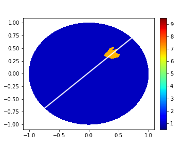
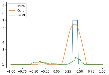
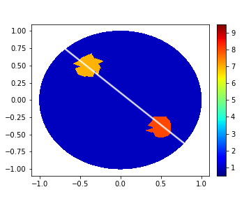
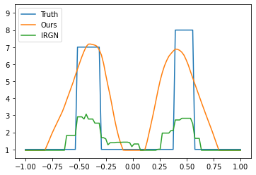
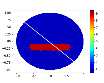
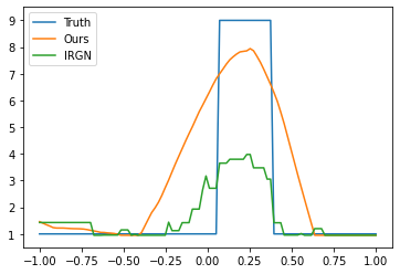
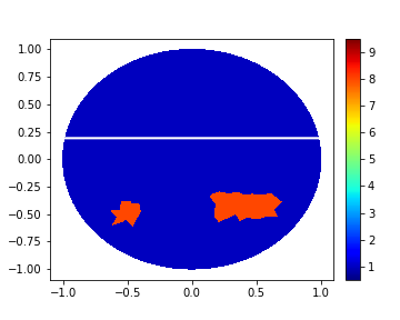
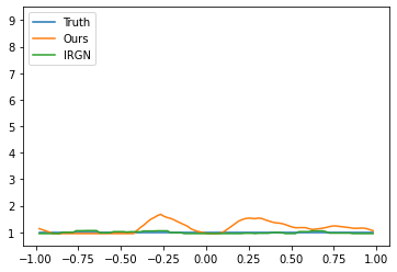
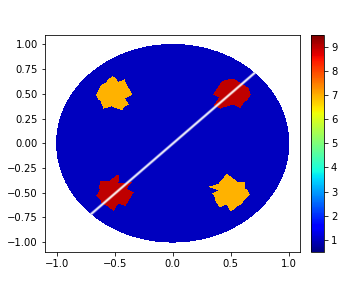
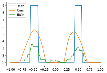
Figure 3: Comparison of reconstructions of our DeepONet with the classical IRGN method. We observe that the DeepONet obtains much closer $\sigma$ values to the ground Truth in the anomalous regions. The white line in the ground truth is the cut at which the plot on the right hand side is displayed.

5.3 Noise Study

The stability of the method against higher noise levels on a single image is evaluated. All experiments of the errors are repeated ten times (On Fig. 3, Row 1) and the mean and standard deviation are displayed in Table LABEL:noise_table. Overall, the $L^{2}$-Error is increasing in a noise pattern in the DeepONet method. The same is true for the IRGN method. However, the IRGN method does have lower $L^{2}$-errors.

We believe that the $L^{2}$ error is not the correct metric because, for images with small anomalous regions, a small error does not imply that the location and conductivity value of the anomaly were estimated properly. For example, in such a case, the reconstruction where everything is exactly the background value, would have relatively low $L^{2}$ errors. However, the reconstruction would not have any practical use. Hence, we use a weighted $L^{2}$ error that takes $50\%$ weight of the ground truth anomalous areas and the rest from the background area. In this metric, the DeepONet method outperforms the IRGN method as expected from seeing the images.

The same patterns in both the weighted and unweighted $L^{2}$ errors are found in all other images that we tested. We note that for large noise levels from $7\%$, the reconstructed anomalies find significantly worse locations and shapes.

Table 3: Noise Study - Fig. 3, Row 1

Noise Level	$1\%$	$2\%$	$3\%$	$4\%$	$5\%$	$9\%$
DeepONet - $L^{2}$ Error	$1.53\pm 0.14$	$1.75\pm 0.31$	$1.78\pm 0.34$	$2.27\pm 0.44$	$2.46\pm 0.85$	$3.86\pm 1.17$
IRGN - $L^{2}$ Error	$0.37\pm 0.02$	$0.42\pm 0.03$	$0.53\pm 0.07$	$0.64\pm 0.11$	$0.81\pm 0.20$	$1.64\pm 0.36$
DeepONet - Weighted $L^{2}$	$0.54\pm 0.52$	$0.63\pm 0.66$	$0.65\pm 0.70$	$0.86\pm 0.96$	$1.05\pm 1.25$	$1.62\pm 2.17$
IRGN - Weighted $L^{2}$	$14.16\pm 0.79$	$14.15\pm 0.98$	$14.34\pm 2.87$	$13.44\pm 2.61$	$14.65\pm 3.75$	$14.21\pm 4.71$

6 Conclusion

In this work, we have generalized the earlier known approximation-theoretic results for approximating a map between infinite-dimensional function spaces using DeepONets to the case where we can provide similar guarantees even when the goal is to learn a map between a space of (N-t-D) operators to the space of conductivities (functions). This map arises naturally in the framework of Electrical Impedance Tomography which is a non-invasive medical imaging modality that is becoming increasingly prominent in especially several neuro-imaging applications. As deep-learning networks are becoming increasingly popular, it behooves us to go beyond black-box description of such networks and to make them interpretable so as to facilitate deployment with confidence in critical applications such as medical imaging. Providing approximation-theoretic guarantees of the kind given in this work is a crucial step in achieving the goal of interpretable neural-networks. In fact, we believe that the analysis carried out in this work can be easily adapted to many other problems wherein the input and output spaces are classes of operators satisfying certain general assumptions. To that end, we have proposed a DeepONet architecture that is motivated by the underlying inverse map appearing in EIT. We have compared our approach against the widely used IRGN benchmark and show that the proposed network outperforms the baseline in numerical studies. We also performed a noise study and show that robustness of the deep-learning based against a weighted $L^{2}$ error metric as introduced in this work. To our knowledge, this is the first work that uses a DeepONet architecture for approximating an operator-to-function map as appearing in EIT, while also providing a theoretical guarantee to show its effectiveness. As already stated, our numerical results back-up our theoretical findings.

7 Appendix

Lemma 3.

The set $D_{\Lambda}$ is a compact set in $\mathbb{H}_{r}$.

Proof.

First of all we note that $\mathbb{H}_{r}$ is a separable Hilbert Space with a countable basis given in [1, section 5.1]. From [63, Theorem 197], it suffices to show that $D_{\Lambda}$ is closed, bounded and has equi-small tails with respect to the orthonormal basis for $\mathbb{H}_{r}$. The fact that $D_{\Lambda}$ is bounded follows from [20, (2.5)] as before. The fact that $D_{\Lambda}$ has equi-small tails follows from [1, Lemma 18] in which we choose $J,K$ and $\nu$ such that $C\min(J,K)^{-\nu}\leq\epsilon$ for any given $\epsilon$. Thus it remains to show that $D_{\Lambda}$ is closed. To that end, choose a sequence of relative N-t-D operators $(\tilde{\Lambda}_{\gamma_{n}}:\gamma_{n}\in\Gamma^{\alpha}_{m,\Omega^{\prime}})$ such that they converge to some operator $T$ in $\mathbb{H}_{r}$ i.e., $\tilde{\Lambda}_{\gamma_{n}}\to T$. We will show that there exists some $\gamma\in\Gamma$ such that $T=\tilde{\Lambda}_{\gamma}$ i.e. $T$ is also a N-t-D operator. First of all note that since $(\tilde{\Lambda}_{\gamma_{n}})$ converges, hence $(\tilde{\Lambda}_{\gamma_{n}})$ is actually Cauchy in the $\mathbb{H}_{r}$ norm. Mimicking the proof of [1, Lemma 5], we can show that $(\Lambda_{\gamma_{n}})$ is also Cauchy in the operator norm $\mathcal{L}(L^{2}\to L^{2})$. By using the inverse continuity result for the Calderon problem, see [27, Theorem 2.3], we get that the sequence $\gamma_{n}$ is Cauchy with respect to the $L^{\infty}$ norm and hence converges, say $\gamma_{n}\to\gamma_{0}\in L^{\infty}(\Omega)\cap\Gamma$. Let us now consider, $\Lambda_{\gamma_{0}}$. From forward continuity result for the Calderon problem, see [27, Lemma 2.5], $\Lambda_{\gamma_{n}}\to\Lambda_{\gamma_{0}}$. Now from uniqueness of the limit, $\Lambda_{\gamma_{0}}=T$. Hence the set, $D_{\Lambda}$ satisfies all theree criteria for it be a compact subset of $\mathbb{H}_{r}$. ∎

Lemma 4.

[16, Theorem 4.1] Let $X$ be an arbitrary metric space, $A$ a closed subset of $X$, $L$ a locally convex linear space, and $f:A\to L$ be a continuous map. Then there exists an extension $F:X\to L$ (which is continuous by definition) such that $F(a)=f(a)$ for all $a\in A$.

7.1 Continuity results of some maps

Consider the encoding map $\mathcal{E}(\tilde{\Lambda}):=\mathcal{E}_{M}(\tilde{\Lambda})=\tilde{R}^{M}_{\gamma}.$ We have the following continuity results:

Lemma 5.

[44, section 2] The map $T:\gamma\to\tilde{R}_{\gamma}^{M}$ is Lipschitz continuous, i.e. $\lvert\lvert\tilde{R}^{M}_{\gamma_{1}}-\tilde{R}^{M}_{\gamma_{2}}\rvert\rvert_{\mathcal{L}(L^{2}\to L^{2})}\leq\lvert\lvert\gamma_{1}-\gamma_{2}\rvert\rvert_{L^{\infty}}$

Lemma 6.

[27, Theorem 2.3] $\lvert\lvert\gamma_{1}-\gamma_{2}\rvert\rvert_{L^{2}}\leq c\lvert\lvert\gamma_{1}-\gamma_{2}\rvert\rvert_{L^{\infty}}\leq C\lvert\lvert\tilde{\Lambda}_{\gamma_{1}}-\tilde{\Lambda}_{\gamma_{2}}\rvert\rvert_{\mathcal{L}(L^{2}\to L^{2})}$

From previous two Lemmas, we get that the map $\mathcal{E}$ is Lipschitz continuous.

References Cited

- [1] Kweku Abraham and Richard Nickl. On statistical Calderón problems. Math. Stat. Learn., 2(2):165–216, 2019.
- [2] J P Agnelli, A Çöl, M Lassas, R Murthy, M Santacesaria, and S Siltanen. Classification of stroke using neural networks in electrical impedance tomography. Inverse Problems, 36(11):115008, oct 2020.
- [3] Sanwar Ahmad, Thilo Strauss, Shyla Kupis, and Taufiquar Khan. Comparison of statistical inversion with iteratively regularized gauss newton method for image reconstruction in electrical impedance tomography. Applied Mathematics and Computation, 358:436–448, 2019.
- [4] Giovanni Alessandrini. Stable determination of conductivity by boundary measurements. Appl. Anal., 27(1-3):153–172, 1988.
- [5] Harri Hakula Armin Lechleiter, Nuutti Hyvoönen. Factorization method applied to the complete electrode model of impedance tomography. SIAM J. Appl. Math, 68(4):1097–1121, 2008.
- [6] Francesca Bartolucci, Emmanuel de Bézenac, Bogdan Raonic, Roberto Molinaro, Siddhartha Mishra, and Rima Alaifari. Representation equivalent neural operators: a framework for alias-free operator learning. In A. Oh, T. Naumann, A. Globerson, K. Saenko, M. Hardt, and S. Levine, editors, Advances in Neural Information Processing Systems, volume 36, pages 69661–69672. Curran Associates, Inc., 2023.
- [7] Liliana Borcea. Electrical impedance tomography. Inverse problems, 18(6):R99, 2002.
- [8] Nikolas Borrel-Jensen, Somdatta Goswami, Allan P. Engsig-Karup, George Em Karniadakis, and Cheol-Ho Jeong. Sound propagation in realistic interactive 3d scenes with parameterized sources using deep neural operators. Proceedings of the National Academy of Sciences, 121(2):e2312159120, 2024.
- [9] Alberto-P. Calderón. On an inverse boundary value problem. In Seminar on Numerical Analysis and its Applications to Continuum Physics (Rio de Janeiro, 1980), pages 65–73. Soc. Brasil. Mat., Rio de Janeiro, 1980.
- [10] T. Chen and H. Chen. Approximations of continuous functionals by neural networks with application to dynamic systems. IEEE Transactions on Neural Networks, 4(6):910–918, 1993.
- [11] Tianping Chen and Hong Chen. Approximation capability to functions of several variables, nonlinear functionals, and operators by radial basis function neural networks. IEEE Transactions on Neural Networks, 6(4):904–910, 1995.
- [12] Tianping Chen and Hong Chen. Universal approximation to nonlinear operators by neural networks with arbitrary activation functions and its application to dynamical systems. IEEE Transactions on Neural Networks, 6(4):911–917, 1995.
- [13] Margaret Cheney, David Isaacson, and Jonathan C Newell. Electrical impedance tomography. SIAM review, 41(1):85–101, 1999.
- [14] V.A. Cherepenin, A.Y. Karpov, A.V. Korjenevsky, V.N. Kornienko, Y.S. Kultiasov, M.B. Ochapkin, O.V. Trochanova, and J.D. Meister. Three-dimensional eit imaging of breast tissues: system design and clinical testing. IEEE Transactions on Medical Imaging, 21(6):662–667, 2002.
- [15] Maarten V. de Hoop, Nikola B. Kovachki, Nicholas H. Nelsen, and Andrew M. Stuart. Convergence rates for learning linear operators from noisy data. SIAM/ASA Journal on Uncertainty Quantification, 11(2):480–513, 2023.
- [16] J. Dugundji. An extension of Tietze’s theorem. Pacific J. Math., 1:353–367, 1951.
- [17] David Isaacson Erkki Somersalo, Margaret Cheney. Existence and uniqueness for electrode models forelectric current computed tomography. SIAM J. APPL. MATH, 52(4):1023–1040, 1992.
- [18] Yuwei Fan and Lexing Ying. Solving electrical impedance tomography with deep learning. Journal of Computational Physics, 404:109119, 2020.
- [19] I. Frerichs, J. Hinz, P. Herrmann, G. Weisser, G. Hahn, M. Quintel, and G. Hellige. Regional lung perfusion as determined by electrical impedance tomography in comparison with electron beam ct imaging. IEEE Transactions on Medical Imaging, 21(6):646–652, 2002.
- [20] Henrik Garde and Nuutti Hyvönen. Mimicking relative continuum measurements by electrode data in two-dimensional electrical impedance tomography. Numer. Math., 147(3):579–609, 2021.
- [21] MATTEO SANTACESARIA GIOVANNI S. ALBERTI. CalderÓn’s inverse problem with a finite ´ number of measurements. Forum of Mathematics, Sigma, 7(e35):20 p.p., 2019.
- [22] Somdatta Goswami, Aniruddha Bora, Yue Yu, and George Em Karniadakis. Physics-informed deep neural operator networks, 2022.
- [23] Sarah J Hamilton, Asko Hänninen, Andreas Hauptmann, and Ville Kolehmainen. Beltrami-net: domain-independent deep d-bar learning for absolute imaging with electrical impedance tomography (a-eit). Physiological measurement, 40(7):074002, 2019.
- [24] Sarah Jane Hamilton and Andreas Hauptmann. Deep d-bar: Real-time electrical impedance tomography imaging with deep neural networks. IEEE transactions on medical imaging, 37(10):2367–2377, 2018.
- [25] Martin Hanke and Martin Brühl. Recent progress in electrical impedance tomography. Inverse Problems, 19(6):S65, 2003.
- [26] Martin Hanke, Nuutti Hyvönen, and Stefanie Reusswig. Convex backscattering support in electric impedance tomography. Numer. Math., 117(2):373–396, 2011.
- [27] Bastian Harrach. Uniqueness and Lipschitz stability in electrical impedance tomography with finitely many electrodes. Inverse Problems, 35(2):024005, 19, 2019.
- [28] QiZhi He, Mauro Perego, Amanda A. Howard, George Em Karniadakis, and Panos Stinis. A hybrid deep neural operator/finite element method for ice-sheet modeling. Journal of Computational Physics, 492:112428, 2023.
- [29] Ping Hu, Bing Shuai, Jun Liu, and Gang Wang. Deep level sets for salient object detection. In Proceedings of the IEEE conference on computer vision and pattern recognition, pages 2300–2309, 2017.
- [30] Nuutti Hyvönen. Approximating idealized boundary data of electric impedance tomography by electrode measurements. Math. Models Methods Appl. Sci., 19(7):1185–1202, 2009.
- [31] David Isaacson, Jennifer L Mueller, Jonathan C Newell, and Samuli Siltanen. Reconstructions of chest phantoms by the d-bar method for electrical impedance tomography. IEEE Transactions on Medical Imaging, 23(7):821–828, 2004.
- [32] Bangti Jin, Taufiquar Khan, and Peter Maass. A reconstruction algorithm for electrical impedance tomography based on sparsity regularization. International Journal for Numerical Methods in Engineering, 89(3):337–353, 2012.
- [33] Bangti Jin and Peter Maass. An analysis of electrical impedance tomography with applications to tikhonov regularization. ESAIM: Control, Optimisation and Calculus of Variations, 18(4):1027–1048, 2012.
- [34] JP Kaipio, A Seppänen, E Somersalo, and H Haario. Posterior covariance related optimal current patterns in electrical impedance tomography. Inverse Problems, 20(3):919, 2004.
- [35] George Em Karniadakis Katiana Kontolati, Somdatta Goswami and Michael D. Shields. Learning nonlinear operators in latent spaces for real-time predictions of complex dynamics in physical systems. Nature Communications, 15.
- [36] Xi-Yang Ke, Wei Hou, Qi Huang, Xue Hou, Xue-Ying Bao, Wei-Xuan Kong, Cheng-Xiang Li, Yu-Qi Qiu, Si-Yi Hu, and Li-Hua Dong. Advances in electrical impedance tomography-based brain imaging. Military Medical Research, 9, 2022.
- [37] Taufiquar Khan and Alexandra Smirnova. 1d inverse problem in diffusion based optical tomography using iteratively regularized gauss–newton algorithm. Applied mathematics and computation, 161(1):149–170, 2005.
- [38] Andreas Kirsch and Natalia Grinberg. The factorization method for inverse problems. Number 36. Oxford University Press, 2008.
- [39] Nikola Kovachki, Samuel Lanthaler, and Siddhartha Mishra. On universal approximation and error bounds for fourier neural operators. Journal of Machine Learning Research, 22(290):1–76, 2021.
- [40] Nikola Kovachki, Zongyi Li, Burigede Liu, Kamyar Azizzadenesheli, Kaushik Bhattacharya, Andrew Stuart, and Anima Anandkumar. Neural operator: Learning maps between function spaces with applications to pdes. Journal of Machine Learning Research, 24(89):1–97, 2023.
- [41] Nikola B. Kovachki, Samuel Lanthaler, and Andrew M. Stuart. Operator learning: Algorithms and analysis, 2024.
- [42] Nikola Borislavov Kovachki. Machine Learning and Scientific Computing. ProQuest LLC, Ann Arbor, MI, 2022. Thesis (Ph.D.)–California Institute of Technology.
- [43] Samuel Lanthaler, Siddhartha Mishra, and George E. Karniadakis. Error estimates for DeepONets: a deep learning framework in infinite dimensions. Trans. Math. Appl., 6(1):tnac001, 141, 2022.
- [44] Armin Lechleiter and Andreas Rieder. Newton regularizations for impedance tomography: convergence by local injectivity. Inverse Problems, 24(6):065009, 18, 2008.
- [45] Zongyi Li, Nikola Kovachki, Kamyar Azizzadenesheli, Burigede Liu, Kaushik Bhattacharya, Andrew Stuart, and Anima Anandkumar. Markov neural operators for learning chaotic systems. arXiv preprint arXiv:2106.06898, pages 2–3, 2021.
- [46] Zongyi Li, Hongkai Zheng, Nikola Kovachki, David Jin, Haoxuan Chen, Burigede Liu, Kamyar Azizzadenesheli, and Anima Anandkumar. Physics-informed neural operator for learning partial differential equations, 2023.
- [47] Zongyi Li, Hongkai Zheng, Nikola Kovachki, David Jin, Haoxuan Chen, Burigede Liu, Kamyar Azizzadenesheli, and Anima Anandkumar. Physics-informed neural operator for learning partial differential equations. ACM / IMS J. Data Sci., 1(3), may 2024.
- [48] William RB Lionheart. Eit reconstruction algorithms: pitfalls, challenges and recent developments. Physiological measurement, 25(1):125, 2004.
- [49] Benyuan Liu, Bin Yang, Canhua Xu, Junying Xia, Meng Dai, Zhenyu Ji, Fusheng You, Xiuzhen Dong, Xuetao Shi, and Feng Fu. pyeit: A python based framework for electrical impedance tomography. SoftwareX, 7:304–308, 2018.
- [50] Lu Lu, Pengzhan Jin, Guofei Pang, Zhongqiang Zhang, and George Em Karniadakis. Learning nonlinear operators via deeponet based on the universal approximation theorem of operators. Nat Mach Intell, 3:218–229, 2021.
- [51] Niculae Mandache. Exponential instability in an inverse problem for the Schrödinger equation. Inverse Problems, 17(5):1435–1444, 2001.
- [52] Lars Mescheder, Michael Oechsle, Michael Niemeyer, Sebastian Nowozin, and Andreas Geiger. Occupancy networks: Learning 3d reconstruction in function space. In Proceedings of the IEEE/CVF Conference on Computer Vision and Pattern Recognition, pages 4460–4470, 2019.
- [53] Ben Mildenhall, Pratul P Srinivasan, Matthew Tancik, Jonathan T Barron, Ravi Ramamoorthi, and Ren Ng. Nerf: Representing scenes as neural radiance fields for view synthesis. In European Conference on Computer Vision, pages 405–421. Springer, 2020.
- [54] Adrian I. Nachman. Global uniqueness for a two-dimensional inverse boundary value problem. Ann. of Math. (2), 143(1):71–96, 1996.
- [55] Richard Nickl, Sara van de Geer, and Sven Wang. Convergence rates for penalized least squares estimators in PDE constrained regression problems. SIAM/ASA J. Uncertain. Quantif., 8(1):374–413, 2020.
- [56] Roman Novikov and Matteo Santacesaria. A global stability estimate for the Gelfand-Calderón inverse problem in two dimensions. J. Inverse Ill-Posed Probl., 18(7):765–785, 2010.
- [57] Michael Oechsle, Lars Mescheder, Michael Niemeyer, Thilo Strauss, and Andreas Geiger. Texture fields: Learning texture representations in function space. In Proceedings of the IEEE/CVF International Conference on Computer Vision, pages 4531–4540, 2019.
- [58] Michael Oechsle, Michael Niemeyer, Christian Reiser, Lars Mescheder, Thilo Strauss, and Andreas Geiger. Learning implicit surface light fields. In 2020 International Conference on 3D Vision (3DV), pages 452–462. IEEE, 2020.
- [59] Ahmad Peyvan, Vivek Oommen, Ameya D. Jagtap, and George Em Karniadakis. Riemannonets: Interpretable neural operators for riemann problems. Computer Methods in Applied Mechanics and Engineering, 426:116996, June 2024.
- [60] Akarsh Pokkunuru, Pedram Rooshenas, Thilo Strauss, Anuj Abhishek, and Taufiquar Khan. Improved training of physics-informed neural networks using energy-based priors: a study on electrical impedance tomography. In The Eleventh International Conference on Learning Representations, 2023.
- [61] Andrea Randazzo, Emanuele Tavanti, Mantas Mikulenas, Federico Boero, Alessandro Fedeli, Andrea Sansalone, Giorgio Allasia, and Matteo Pastorino. An electrical impedance tomography system for brain stroke imaging based on a lebesgue-space inversion procedure. IEEE Journal of Electromagnetics, RF and Microwaves in Medicine and Biology, 5(1):54–61, 2021.
- [62] Bogdan Raonic, Roberto Molinaro, Tim De Ryck, Tobias Rohner, Francesca Bartolucci, Rima Alaifari, Siddhartha Mishra, and Emmanuel de Bézenac. Convolutional neural operators for robust and accurate learning of pdes. In A. Oh, T. Naumann, A. Globerson, K. Saenko, M. Hardt, and S. Levine, editors, Advances in Neural Information Processing Systems, volume 36, pages 77187–77200. Curran Associates, Inc., 2023.
- [63] Casey Rodriguez and Andrew Lin. Lecture notes on Basic Functional Analysis. MIT OCW, 2020.
- [64] M Salo. Calderon problem lecture notes. 2008.
- [65] Benjamin Shih, Ahmad Peyvan, Zhongqiang Zhang, and George Em Karniadakis. Transformers as neural operators for solutions of differential equations with finite regularity, 2024.
- [66] Vincent Sitzmann, Julien Martel, Alexander Bergman, David Lindell, and Gordon Wetzstein. Implicit neural representations with periodic activation functions. In H. Larochelle, M. Ranzato, R. Hadsell, M.F. Balcan, and H. Lin, editors, Advances in Neural Information Processing Systems, volume 33, pages 7462–7473. Curran Associates, Inc., 2020.
- [67] Thilo Strauss and Taufiquar Khan. Statistical inversion in electrical impedance tomography using mixed total variation and non-convex regularization prior. Journal of Inverse and Ill-posed Problems, 23(5):529–542, 2015.
- [68] Thilo Strauss and Taufiquar Khan. Implicit solutions of the electrical impedance tomography inverse problem in the continuous domain with deep neural networks. Entropy, 25(3):493, 2023.
- [69] John Sylvester and Gunther Uhlmann. A uniqueness theorem for an inverse boundary value problem in electrical prospection. Comm. Pure Appl. Math., 39(1):91–112, 1986.
- [70] G. Uhlmann. Electrical impedance tomography and Calderón’s problem. Inverse Problems, 25(12):123011, 39, 2009.
- [71] Anna Witkowska-Wrobel, Kirill Aristovich, Mayo Faulkner, James Avery, and David Holder. Feasibility of imaging epileptic seizure onset with eit and depth electrodes. NeuroImage, 173:311–321, 2018.
- [72] Bin Yang, Bing Li, Canhua Xu, Shijie Hu, Meng Dai, Junying Xia, Peng Luo, Xuetao Shi, Zhanqi Zhao, Xiuzhen Dong, Zhou Fei, and Feng Fu. Comparison of electrical impedance tomography and intracranial pressure during dehydration treatment of cerebral edema. NeuroImage: Clinical, 23:101909, 2019.
- [73] Dmitry Yarotsky. Error bounds for approximations with deep relu networks. Neural Networks, 94:103–114, 2017.
- [74] Min Zhu, Handi Zhang, Anran Jiao, George Em Karniadakis, and Lu Lu. Reliable extrapolation of deep neural operators informed by physics or sparse observations. Computer Methods in Applied Mechanics and Engineering, 412:116064, 2023.